Batch Informed Trees (BIT*): Sampling-based Optimal Planning via the Heuristically Guided Search of Implicit Random Geometric Graphs

Abstract

In this paper, we present Batch Informed Trees (BIT*), a planning algorithm based on unifying graph- and sampling-based planning techniques. By recognizing that a set of samples describes an implicit random geometric graph (RGG), we are able to combine the efficient ordered nature of graph-based techniques, such as A*, with the anytime scalability of sampling-based algorithms, such as Rapidly-exploring Random Trees.

BIT* uses a heuristic to efficiently search a series of increasingly dense implicit RGGs while reusing previous information. It can be viewed as an extension of incremental graph-search techniques, such as Lifelong Planning A* (LPA*), to continuous problem domains as well as a generalization of existing sampling-based optimal planners. It is shown that it is probabilistically complete and asymptotically optimal.

We demonstrate the utility of BIT* on simulated random worlds in $\mathbb{R}^{2}$ and $\mathbb{R}^{8}$ and manipulation problems on CMU’s HERB, a 14-DOF two-armed robot. On these problems, BIT* finds better solutions faster than RRT, RRT*, Informed RRT*, and Fast Marching Trees (FMT*) with faster anytime convergence towards the optimum, especially in high dimensions.

I Introduction

Graph-search and sampling-based methods are two popular techniques for path planning in robotics. Graph-based searches, such as Dijkstra’s algorithm [1] and A* [2], use dynamic programming [3] to exactly solve a discrete approximation of a problem. These algorithms are not only resolution complete but also resolution optimal, always finding the optimal solution to the given problem at the chosen discretization, if one exists. A* does this efficiently by using a heuristic to estimate the total cost of a solution constrained to pass through a state. The result is an algorithm that searches in order of decreasing solution quality and is optimally efficient. Any other optimal algorithm using the same heuristic will expand at least as many vertices as A* [2].

The quality of the continuous solution found by these graph-search techniques depends heavily on the discretization of the problem. Finer discretization increases the quality of the solution [4], but also increases the computational effort necessary to find it. This becomes a significant problem in high-dimensional spaces, such as for manipulation planning (Fig. 1), as the size of the discrete state space grows exponentially with the number of dimensions. Bellman [5] referred to this problem as the curse of dimensionality. Graph-search techniques have still been successful as planning algorithms [6] on a variety of graph types [7, 8], including for nonholonomoic robots [9, 10], kinodynamic planning [11, 12], and manipulation planning [13].

Graph search has also been extended to anytime and incremental search. Anytime techniques [14, 15, 16] quickly find a suboptimal path before completing the search for the optimum, while incremental techniques [17, 18, 19, 15, 16] handle changes in a graph efficiently by reusing information.

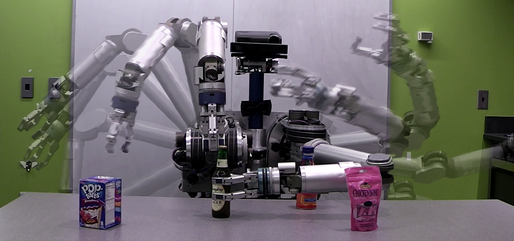
Figure 1: A composite figure of a trajectory generated by BIT* for a difficult $14$-DOF two-arm manipulation planning problem on HERB. In the trial pictured, BIT* found a solution in $4$ seconds and spent $2.5$ minutes refining it. Over $25$ trials with $2.5$ minutes of computational time, BIT* had a median solution cost of $17.4$ and success rate of $68\%$, while Informed RRT* and FMT* had median costs of $25.3$ and $17.2$ and success rates of $8\%$ and $36\%$, respectively. Nonoptimal planners, RRT and RRT-Connect, had median costs of $31.1$ and $22.1$ and success rates of $8\%$ and $100\%$, respectively.

Sampling-based planners, such as PRM [20], RRT [21], and Expansive Space Trees [22], avoid the discretization problems of graph-search techniques by randomly sampling the continuous planning domain. This scales more effectively to high-dimensional problems, but makes their search probabilistic. They are probabilistically complete, having a probability of finding a solution, if one exists, that goes to one as the number of samples goes to infinity. Anytime algorithms, such as RRT and EST, also have anytime resolution, a growing representation of the problem domain that becomes increasingly accurate as the number of iterations increases. Optimal variants, such as RRT* and PRM* [23], are also asymptotically optimal, converging asymptotically to the optimal solution with probability one as the number of samples goes to infinity (almost sure asymptotic convergence). While solutions improve with computational time, this does not guarantee a reasonable rate of convergence as the random sampling is inherently unordered.

There is a long history of adding graph-search concepts to sampling-based planners. Algorithms have used heuristics to refine the RRT search, including by biasing the sampling procedure [24], and to define a series of subplanning problems given the current solution [25]. Similarly, focusing techniques have also been used to limit the search of optimal (RRT*) once it finds a solution [26, 27, 28]. While these techniques can improve the initial solution and/or the convergence rate to the optimum, their RRT-based search is still unordered.

Other algorithms order the search at the expense of anytime resolution. FMT* [29] uses a marching method to process a single set of samples. The resulting search is ordered on cost-to-come but must be restarted if a higher resolution is needed. The Motion Planning Using Lower Bounds (MPLB) algorithm [30] extends FMT* to quasi-anytime resolution and an ordering given by estimating the cost of solutions constrained to pass through each state. The quasi-anytime resolution is achieved by solving a series of independent problems with an increasing number of samples. It is stated that this can be done efficiently by reusing information, but no specific methods are presented.

Still other algorithms attempt to extend graph-search directly to continuous planning problems. In Randomized A* (RA*) [31] and Sampling-based A* (SBA*) [32] a tree is grown towards solutions by sampling near heuristically selected vertices. This biases the growth of the tree towards good solutions but requires methods to avoid local minima. RA* defines a minimum-allowed distance between vertices, limiting the number of times a vertex can be expanded but also limiting the final resolution. SBA* includes a measure of local sample density in the vertex expansion heuristic. This decreases the priority of sampling near frequently expanded vertices, but requires methods to estimate local sample density.

In this paper, we present BIT*, a planning algorithm that balances the benefits of graph-search and sampling-based techniques. It uses batches of samples to perform an ordered search on a continuous planning domain while maintaining anytime performance. By processing samples in batches, its search can be ordered around the minimum solution proposed by a heuristic, as in A* [2]. By processing multiple batches of samples, it converges asymptotically towards the global optimum with anytime resolution, as in RRT* [23]. This is done efficiently by using incremental search techniques to incorporate the new samples into the existing search, as in LPA* [17]. The multiple batches also allow subsequent searches to be focused on the subproblem that could contain a better solution, as in Informed RRT* [28].

The performance of BIT* is demonstrated both on random experiments in $\mathbb{R}^{2}$ and $\mathbb{R}^{8}$ and manipulation problems on the CMU Personal Robotic Lab’s Home Exploring Robot Butler (HERB) [33]. The results show that BIT* consistently outperformed both nonasymptotically and asymptotitcally optimal planners (RRT, RRT*, Informed RRT*, and FMT*). It was more likely to have found a solution at a given computational time and converged towards the optimum faster. The same held in difficult planning problems on HERB, where collision checking is expensive. BIT* was nearly twice as likely to find a solution to a difficult two-arm problem (Fig. 1) and found better solutions on easier one-arm problems (Fig. 6). The only planner tested that found solutions faster was RRT-Connect, which does not converge towards the optimum.

The remainder of this paper is organized as follows. Section II presents further background and Section III presents a description of the algorithm. Section IV presents an initial theoretical analysis of BIT*, while Section V presents the experimental results in detail. Finally, Section VI presents a discussion on the algorithm and related future work and Section VII provides a conclusion.

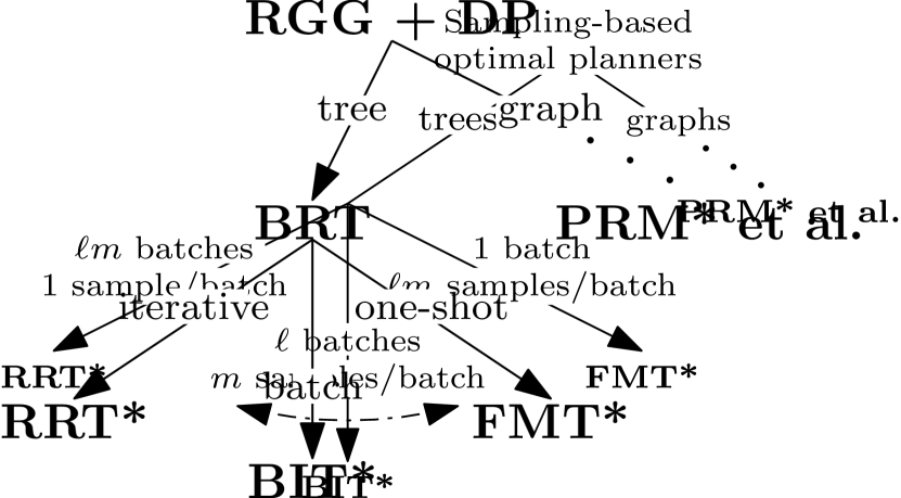
Figure 2: A simplified taxonomy of sampling-based optimal planners demonstrating the relationship between RRT*, FMT*, and BIT*.

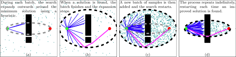
Figure 3: An illustration of the informed search procedure used by BIT*. The start and goal states are shown as green and red, respectively. The current solution is highlighted in magenta. The subproblem that contains any better solutions is shown as a black dashed line, while the progress of the current batch is shown as a grey dashed line. Fig. (a) shows the growing search of the first batch of samples, and (b) shows the first search ending when a solution is found. After pruning and adding a second batch of samples, Fig. (c) shows the search restarting on a denser graph while (d) shows the second search ending when an improved solution is found. An animated illustration is available in the attached video.

II Background

We define the optimal planning problem similarly to [23].

Problem Definition 1 (Optimal Planning)

Let $X\subseteq\mathbb{R}^{n}$ be the state space of the planning problem, $X_{\rm obs}\subset X$ be the states in collision with obstacles, and $X_{\rm free}=X\setminus X_{\rm obs}$ be the resulting set of permissible states. Let $\mathbf{x}_{\rm start}\in X_{\rm free}$ be the initial state and $X_{\rm goal}\subset X_{\rm free}$ be the set of desired final states. Let $\sigma:\;\left[0,1\right]\mapsto X$ be a sequence of states (a path) and $\Sigma$ be the set of all nontrivial paths.

The optimal solution is the path, $\sigma^{*}$, that minimizes a chosen cost function, $s:\;\Sigma\mapsto\mathbb{R}_{\geq 0}$, while connecting $\mathbf{x}_{\rm start}$ to any $\mathbf{x}_{\rm goal}\in X_{\rm goal}$ through free space,

$$\textstyle\sigma^{*}=\operatorname*{arg\,min}\limits_{\sigma\in\Sigma}\left\{s\left(\sigma\right)\;\;\middle|\;\;\right. \sigma(0)=\mathbf{x}_{\rm start},\,\sigma(1)\in\mathbf{x}_{\rm goal},$$

$$\quad\left.\forall t\in\left[0,1\right],\,\sigma\left(t\right)\in X_{\rm free}\right\},$$

where $\mathbb{R}_{\geq 0}$ is the set of non-negative real numbers. We denote the cost of this optimal path as $s^{*}$. ∎

A discrete set of states in this state space, $X_{\rm samples}\subset X$, can be viewed as a graph whose edges are given algorithmically by a transition function (an implicit graph). When these states are sampled randomly, $X_{\rm samples}=\left\{\mathbf{x}\sim\mathcal{U}\left(X\right)\right\}$, the properties of the graph can be described by a probabilistic model known as a RGG [34].

In an RGG, the connections (edges) between states (vertices) depend on their relative geometric position. Common RGGs have edges to a specific number of each state’s nearest neighbours (a $k$-nearest graph [35]) or to all neighbours within a specific distance (an $r$-disc graph [36]). RGG theory provides probabilistic relationships between the number and distribution of samples, the $k$ or $r$ defining the graph, and specific graph properties such as connectivity or relative cost through the graph [34, 37, 23, 29].

Sampling-based planners can therefore be viewed as algorithms to construct an implicit RGG and an explicit spanning tree in the free space of the planning problem. Much like graph-search techniques, the performance of an algorithm will depend on the quality of the RGG representation and the efficiency of the search.

Karaman and Frazzoli [23] use RGG theory in RRT* to limit graph complexity while maintaining probabilistic bounds on the representation, but the graph is constructed and searched simultaneously, resulting in a randomly ordered anytime search. Janson and Pavone [29] similarly use RGG theory in FMT*, but for a constant number of samples, resulting in an ordered but nonanytime (in solution or resolution) search. Recently, Salzman and Halperin [30] have given FMT* quasi-anytime performance by independently solving increasingly dense RGGs in their MPLB algorithm. Heuristics order and focus the search, but solutions are only returned when an RGG is completely searched.

In contrast, BIT* uses incremental search techniques on increasingly dense RGGs. This balances the benefits of heuristically ordered search with anytime performance and asymptotic optimality. The tuning parameters are the choice of the heuristic, an RGG constant, and the number of samples per batch. BIT* can be viewed as an extension of LPA* [17] to continuous problems and as a generalization of existing sampling-based optimal planners (Fig. 2). With batches of one sample, it is a version of Informed RRT* [28], and with a single batch and the zero heuristic, a version of FMT*.

III Batch Informed Trees (BIT*)

Informally, BIT* works as follows. An initial RGG with implicit edges is defined by uniformly distributed random samples from the free space and the start and goal. The RGG parameter ($r$ or $k$) is chosen to reduce graph complexity while maintaining asymptotic optimality requirements as a function of the number of samples [23, 29]. An explicit tree is then built outwards from the start towards the goal by a heuristic search (Fig. 3a). This tree includes only collision-free edges and its construction stops when a solution is found or it can no longer be expanded (Fig. 3b). This concludes a batch.

To start a new batch, a denser implicit RGG is constructed by adding more samples and updating $r$ (or $k$). If a solution has been found, these samples are limited to the subproblem that could contain a better solution (e.g., an ellipse for path length [28]). The tree is then updated using LPA*-style incremental search techniques that reuse existing information (Fig. 3c). As before, the construction of the tree stops when the solution cannot be improved or when there are no more collision-free edges to traverse (Fig. 3d). The process continues with new batches as time allows.

III-A Notation

The functions $\widehat{g}\left(\mathbf{x}\right)$ and $\widehat{h}\left(\mathbf{x}\right)$ represent admissible estimates of the cost-to-come to a state, $\mathbf{x}\in X$, from the start and the cost-to-go from a state to the goal, respectively (i.e., they bound the true costs from below). The function, $\widehat{f}\left(\mathbf{x}\right)$, represents an admissible estimate of the cost of a path from $\mathbf{x}_{\rm start}$ to $X_{\rm goal}$ constrained to pass through $\mathbf{x}$, i.e., $\widehat{f}\left(\mathbf{x}\right):=\widehat{g}\left(\mathbf{x}\right)+\widehat{h}\left(\mathbf{x}\right)$. This estimate defines a subset of states, $X_{\widehat{f}}:=\left\{\mathbf{x}\in X\;\;\middle|\;\;\widehat{f}\left(\mathbf{x}\right)\leq c_{\rm best}\right\}$, that could provide a solution better than the current best solution cost, $c_{\rm best}$.

Let $\mathcal{T}:=\left(V,E\right)$ be an explicit tree with a set of vertices, $V\subset X_{\rm free}$, and edges, $E=\left\{\left(\mathbf{v},\mathbf{w}\right)\right\}$ for some $\mathbf{v},\,\mathbf{w}\in V$. The function $g_{\mathcal{T}}\left(\mathbf{x}\right)$ represents the cost-to-come to a state $\mathbf{x}\in X$ from the start vertex given the current tree, $\mathcal{T}$. We assume a state not in the tree, or otherwise unreachable from the start, has a cost-to-come of infinity. It is important to recognize that these two functions will always bound the unknown true optimal cost to a state, $g\left(\cdot\right)$, i.e., $\forall\mathbf{x}\in X,\,\widehat{g}\left(\mathbf{x}\right)\leq g\left(\mathbf{x}\right)\leq g_{\mathcal{T}}\left(\mathbf{x}\right)$.

The functions $\widehat{c}\left(\mathbf{x},\mathbf{y}\right)$ and $c\left(\mathbf{x},\mathbf{y}\right)$ represent an admissible estimate of the cost of an edge and the true cost of an edge between states $\mathbf{x},\,\mathbf{y}\in X$, respectively. We assume that edges that intersect the obstacle set have a cost of infinity, and therefore $\forall\mathbf{x},\,\mathbf{y}\in X,\,\,\widehat{c}\left(\mathbf{x},\mathbf{y}\right)\leq c\left(\mathbf{x},\mathbf{y}\right)\leq\infty$. It is important to recognize that calculating $c\left(\mathbf{x},\mathbf{y}\right)$ can be expensive (e.g., collision detection, differential constraints, etc.) and using a heuristic estimate for edge cost has the effect of delaying this calculation until necessary.

The function $\lambda\left(\cdot\right)$ represents the Lebesgue measure of a set (e.g., the volume), and $\zeta_{n}$ represent the Lebesgue measure of an $n$-dimensional unit ball. The cardinality of a set is denoted by $\left|\cdot\right|$. We use the notation $X\xleftarrow{\scriptscriptstyle+}\left\{\mathbf{x}\right\}$ and $X\xleftarrow{\scriptscriptstyle-}\left\{\mathbf{x}\right\}$ to compactly represent the compounding operations $X\leftarrow X\cup\left\{\mathbf{x}\right\}$ and $X\leftarrow X\setminus\left\{\mathbf{x}\right\}$, respectively. As is customary, we take the minimum of an empty set to be infinity.

1 $V\leftarrow\left\{\mathbf{x}_{\rm start}\right\};\;$ $E\leftarrow\emptyset;\;$ $X_{\rm samples}\leftarrow\left\{\mathbf{x}_{\rm goal}\right\}$;

2 $\mathcal{Q}_{E}\leftarrow\emptyset;\;$ $\mathcal{Q}_{V}\leftarrow\emptyset;\;$ $r\leftarrow\infty$;

3 repeat

4       if $\mathcal{Q}_{E}\equiv\emptyset\;\mathbf{and}\;\mathcal{Q}_{V}\equiv\emptyset$ then

5             $\mathtt{Prune}\left(g_{\mathcal{T}}\left(\mathbf{x}_{\rm goal}\right)\right)$;

6             $X_{\rm samples}\xleftarrow{\scriptscriptstyle+}\mathtt{Sample}\left(m,g_{\mathcal{T}}\left(\mathbf{x}_{\rm goal}\right)\right)$;

7             $V_{\rm old}\leftarrow V$;

8             $\mathcal{Q}_{V}\leftarrow V$;

9             $r\leftarrow\mathtt{radius}\left(\left|V\right|+\left|X_{\rm samples}\right|\right)$;

10            

11      

12      while $\mathtt{BestQueueValue}\left(\mathcal{Q}_{V}\right)\leq\mathtt{BestQueueValue}\left(\mathcal{Q}_{E}\right)$ do

13             $\mathtt{ExpandVertex}\left(\mathtt{BestInQueue}\left(\mathcal{Q}_{V}\right)\right)$;

14            

15      

16      $\left(\mathbf{v}_{\rm m},\mathbf{x}_{\rm m}\right)\leftarrow\mathtt{BestInQueue}\left(\mathcal{Q}_{E}\right)$;

17       $\mathcal{Q}_{E}\xleftarrow{\scriptscriptstyle-}\left\{\left(\mathbf{v}_{\rm m},\mathbf{x}_{\rm m}\right)\right\}$;

18       if $g_{\mathcal{T}}\left(\mathbf{v}_{\rm m}\right)+\widehat{c}\left(\mathbf{v}_{\rm m},\mathbf{x}_{\rm m}\right)+\widehat{h}\left(\mathbf{x}_{\rm m}\right)<g_{\mathcal{T}}\left(\mathbf{x}_{\rm goal}\right)$ then

19             if $\widehat{g}\left(\mathbf{v}_{\rm m}\right)+c\left(\mathbf{v}_{\rm m},\mathbf{x}_{\rm m}\right)+\widehat{h}\left(\mathbf{x}_{\rm m}\right)<g_{\mathcal{T}}\left(\mathbf{x}_{\rm goal}\right)$ then

20                   if $g_{\mathcal{T}}\left(\mathbf{v}_{\rm m}\right)+c\left(\mathbf{v}_{\rm m},\mathbf{x}_{\rm m}\right)<g_{\mathcal{T}}\left(\mathbf{x}_{\rm m}\right)$ then

21                         if $\mathbf{x}_{\rm m}\in V$ then

22                               $E\xleftarrow{\scriptscriptstyle-}\left\{\left(\mathbf{v},\mathbf{x}_{\rm m}\right)\in E\right\}$;

23                              

24                         else

25                               $X_{\rm samples}\xleftarrow{\scriptscriptstyle-}\left\{\mathbf{x}_{\rm m}\right\}$;

26                               $V\xleftarrow{\scriptscriptstyle+}\left\{\mathbf{x}_{\rm m}\right\};\;$ $\mathcal{Q}_{V}\xleftarrow{\scriptscriptstyle+}\left\{\mathbf{x}_{\rm m}\right\}$;

27                              

28                         $E\xleftarrow{\scriptscriptstyle+}\left\{\left(\mathbf{v}_{\rm m},\mathbf{x}_{\rm m}\right)\right\}$;

29                         $\mathcal{Q}_{E}\xleftarrow{\scriptscriptstyle-}\left\{\left(\mathbf{v},\mathbf{x}_{\rm m}\right)\in\mathcal{Q}_{E}\;\;\middle|\vphantom{g_{\mathcal{T}}\left(\mathbf{v}\right)+\widehat{c}\left(\mathbf{v},\mathbf{x}_{\rm m}\right)\geq g_{\mathcal{T}}\left(\mathbf{x}_{\rm m}\right)}\right.$

                         $\qquad\qquad\qquad\;\left.\vphantom{\left(\mathbf{v}\in V,\mathbf{x}_{\rm m}\right)\in\mathcal{Q}_{E}}g_{\mathcal{T}}\left(\mathbf{v}\right)+\widehat{c}\left(\mathbf{v},\mathbf{x}_{\rm m}\right)\geq g_{\mathcal{T}}\left(\mathbf{x}_{\rm m}\right)\right\}$;

30                        

31                  

32            

33       else

34             $\mathcal{Q}_{E}\leftarrow\emptyset;\;$ $\mathcal{Q}_{V}\leftarrow\emptyset$;

35            

36      

37until $\mathtt{STOP}$;

38return $\mathcal{T}$;

Algorithm 1 BIT*$\left(\mathbf{x}_{\rm start}\in X_{\rm free},\mathbf{x}_{\rm goal}\in X_{\rm goal}\right)$

III-B Algorithm

BIT* is presented in Algs. 1–3. For simplicity, we limit our discussion to a search from the start to a single goal state using an $r$-disc RGG, but the formulation is similar for searches from a goal state, with a goal set, or with a $k$-nearest RGG. The algorithm starts with a given initial state, $\mathbf{x}_{\rm start}$, in the tree, $\mathcal{T}$, and the goal state, $\mathbf{x}_{\rm goal}$, in the set of unconnected samples, $X_{\rm samples}$ (Alg. 1, Line 1). The tree is grown towards $\mathbf{x}_{\rm goal}$ from $\mathbf{x}_{\rm start}$ by processing a queue of RGG edges, $\mathcal{Q}_{E}$. This edge queue is populated by a vertex expansion queue, $\mathcal{Q}_{V}$ (Alg. 1, Line 1).

III-B1 Batch creation (Alg. 1, Lines 1–1)

A new batch begins when the queues are empty. The samples and spanning tree are pruned of states that cannot improve the solution (Alg. 1, Line 1; Alg. 3). A new set of $m$ samples is then added to the RGG from the subproblem containing a better solution (Alg. 1, Line 1). This can be accomplished by rejection sampling or, for some cost functions, direct sampling [28]. The vertices in the tree are labelled so that only connections to new states will be considered (Alg. 1, Line 1) and requeued for expansion (Alg. 1, Line 1). The radius of the underlying $r$-disc RGG is updated to reflect its size, $q$, (Alg. 1, Line 1),

$$\textstyle\mathtt{radius}\left(q\right):=2\eta\left(1+\frac{1}{n}\right)^{\frac{1}{n}}\left(\frac{\lambda\left(X_{\widehat{f}}\right)}{\zeta_{n}}\right)^{\frac{1}{n}}\left(\frac{\log\left(q\right)}{q}\right)^{\frac{1}{n}},$$ (1)

where $\eta\geq 1$ is a tuning parameter [23].

1 $\mathcal{Q}_{V}\xleftarrow{\scriptscriptstyle-}\left\{\mathbf{v}\right\}$;

2 $X_{\rm near}\leftarrow\left\{\mathbf{x}\in X_{\rm samples}\;\;\middle|\;\;\left|\left|\mathbf{x}-\mathbf{v}\right|\right|_{2}\leq r\right\}$;

3 $\mathcal{Q}_{E}\xleftarrow{\scriptscriptstyle+}\left\{\left(\mathbf{v},\mathbf{x}\right)\in V\times X_{\rm near}\;\;\middle|\;\;\vphantom{\widehat{g}\left(\mathbf{v}\right)+\widehat{c}\left(\mathbf{v},\mathbf{x}\right)+\widehat{h}\left(\mathbf{x}\right)<g_{\mathcal{T}}\left(\mathbf{x}_{\rm goal}\right)}\right.$

$\qquad\qquad\qquad\qquad\quad\left.\vphantom{\mathcal{Q}_{E}\xleftarrow{\scriptscriptstyle+}\left(\mathbf{v}\in V,\mathbf{x}\in X_{\rm near}\right)}\widehat{g}\left(\mathbf{v}\right)+\widehat{c}\left(\mathbf{v},\mathbf{x}\right)+\widehat{h}\left(\mathbf{x}\right)<g_{\mathcal{T}}\left(\mathbf{x}_{\rm goal}\right)\right\}$;

4

5if $\mathbf{v}\not\in V_{\rm old}$ then

6       $V_{\rm near}\leftarrow\left\{\mathbf{w}\in V\;\;\middle|\;\;\left|\left|\mathbf{w}-\mathbf{v}\right|\right|_{2}\leq r\right\}$;

7       $\mathcal{Q}_{E}\xleftarrow{\scriptscriptstyle+}\left\{\left(\mathbf{v},\mathbf{w}\right)\in V\times V_{\rm near}\;\;\big{|}\;\;\left(\mathbf{v},\mathbf{w}\right)\not\in E,\vphantom{\widehat{g}\left(\mathbf{v}\right)+\widehat{c}\left(\mathbf{v},\mathbf{w}\right)+\widehat{h}\left(\mathbf{w}\right)<g_{\mathcal{T}}\left(\mathbf{x}_{\rm goal}\right),g_{\mathcal{T}}\left(\mathbf{v}\right)+\widehat{c}\left(\mathbf{v},\mathbf{w}\right)+<g_{\mathcal{T}}\left(\mathbf{w}\right)}\right.$

       $\qquad\qquad\qquad\qquad\widehat{g}\left(\mathbf{v}\right)+\widehat{c}\left(\mathbf{v},\mathbf{w}\right)+\widehat{h}\left(\mathbf{w}\right)<g_{\mathcal{T}}\left(\mathbf{x}_{\rm goal}\right),$

       $\qquad\qquad\qquad\qquad\qquad\qquad\left.\vphantom{\mathcal{Q}_{E}\xleftarrow{\scriptscriptstyle+}\left(\mathbf{v}\in V,\mathbf{w}\in V_{\rm near}\right)\left(\mathbf{v},\mathbf{w}\right)\not\in E,\;\widehat{g}\left(\mathbf{v}\right)+\widehat{c}\left(\mathbf{v},\mathbf{w}\right)+\widehat{h}\left(\mathbf{w}\right)<g_{\mathcal{T}}\left(\mathbf{x}_{\rm goal}\right)}g_{\mathcal{T}}\left(\mathbf{v}\right)+\widehat{c}\left(\mathbf{v},\mathbf{w}\right)<g_{\mathcal{T}}\left(\mathbf{w}\right)\right\}$;

8      

Algorithm 2 ExpandVertex$\left(\mathbf{v}\in\mathcal{Q}_{V}\subseteq V\right)$

1 $X_{\rm samples}\xleftarrow{\scriptscriptstyle-}\left\{\mathbf{x}\in X_{\rm samples}\;\;\middle|\;\;\widehat{f}\left(\mathbf{x}\right)\geq c\right\}$;

2 $V\xleftarrow{\scriptscriptstyle-}\left\{\mathbf{v}\in V\;\;\middle|\;\;\widehat{f}\left(\mathbf{v}\right)>c\right\}$;

3 $E\xleftarrow{\scriptscriptstyle-}\left\{\left(\mathbf{v},\mathbf{w}\right)\in E\;\;\middle|\;\;\widehat{f}\left(\mathbf{v}\right)>c,\;\mathtt{or}\;\widehat{f}\left(\mathbf{w}\right)>c\right\}$;

4 $X_{\rm samples}\xleftarrow{\scriptscriptstyle+}\left\{\mathbf{v}\in V\;\;\middle|\;\;g_{\mathcal{T}}\left(\mathbf{v}\right)\equiv\infty\right\}$;

5 $V\xleftarrow{\scriptscriptstyle-}\left\{\mathbf{v}\in V\;\;\middle|\;\;g_{\mathcal{T}}\left(\mathbf{v}\right)\equiv\infty\right\}$;

Algorithm 3 Prune$\left(c\in\mathbb{\mathbb{missing}}{R}_{\geq 0}\right)$

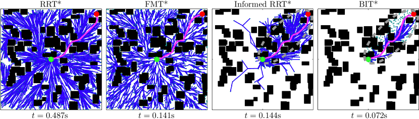
Figure 4: An example of RRT*, Informed RRT*, FMT* ($m=2500$), and BIT* run on a random $\mathbb{R}^{2}$ world. Each algorithm was run until it found a equivalent solution to FMT* ($c=1.39$) regardless of homotopy class. BIT*’s use of heuristics allows it to find such a solution faster ($t=0.072$s) than RRT* ($t=0.487$s), FMT* ($t=0.141$s) and Informed RRT* ($t=0.144$s) by performing its search in a principled manner that initially investigates low-cost solutions and focuses the search for improvements. Animated results are available in the attached video.

III-B2 Edge selection (Alg. 1, Lines 1–1)

The tree is built by processing the queue of edges, $\mathcal{Q}_{E}$, in order of increasing estimated cost of a solution constrained to pass through the edge, $\left(\mathbf{v},\mathbf{x}\right)$, given the current tree, $g_{\mathcal{T}}\left(\mathbf{v}\right)+\widehat{c}\left(\mathbf{v},\mathbf{x}\right)+\widehat{h}\left(\mathbf{x}\right)$. Ties are broken in favour of the edge with the lowest current cost-to-come to the source vertex, $g_{\mathcal{T}}\left(\mathbf{v}\right)$. The function $\mathtt{BestInQueue}\left(\mathcal{Q}_{E}\right)$ returns the best edge in the queue given this ordering. The function $\mathtt{BestQueueValue}\left(\mathcal{Q}_{E}\right)$ returns the estimated solution cost of the best edge in the queue.

The cost of creating the edge queue is delayed by using a vertex expansion queue, $\mathcal{Q}_{V}$. This vertex queue is ordered on the estimated cost of a solution constrained to pass through the vertex given the current tree, $g_{\mathcal{T}}\left(\mathbf{v}\right)+\widehat{h}\left(\mathbf{v}\right)$. This value is a lower bound estimate of the edge-queue values from a vertex; therefore, vertices only need to be expanded into the edge queue when their vertex-queue value is less than the best edge-queue value. The function $\mathtt{BestInQueue}\left(\mathcal{Q}_{V}\right)$ returns the best vertex in the vertex queue given this ordering. The function $\mathtt{BestQueueValue}\left(\mathcal{Q}_{V}\right)$ returns the estimated solution cost of the best vertex in the queue.

Before selecting the next edge in the queue to process, any vertices that could have a better outgoing edge (Alg. 1, Line 1) are expanded (Alg. 1, Line 1; Alg. 2). The best edge in the queue, $\left(\mathbf{v}_{\rm m},\mathbf{x}_{\rm m}\right)$, is then removed for processing (Alg. 1, Lines 1–1). As edges are only added to the edge queue by expanding their source vertex, and each vertex is only expanded once per batch, each edge is guaranteed to only be processed once per batch.

III-B3 Edge processing (Alg. 1, Lines 1–1)

Heuristics are used to accelerate the processing of edges and delay the calculation of the true edge cost. The edge being processed, $\left(\mathbf{v}_{\rm m},\mathbf{x}_{\rm m}\right)$, is first checked to see if it can improve the current solution given the current tree (Alg. 1, Line 1). If it cannot, then by construction no other edges in the queue can and both queues are cleared to start a new batch (Alg. 1, Line 1).

The true edge cost is then calculated by performing collision checks and solving any differential constraints. This may be expensive, so the edge is processed if it could ever improve the current solution, regardless of the current state of the tree (Alg. 1, Line 1). If it cannot, than it is discarded.

Finally, the edge is checked to see if it improves the cost-to-come of its target vertex (Alg. 1, Line 1), noting that disconnected vertices have an infinite cost. If it does, it is added to the tree.

If the target vertex, $\mathbf{x}_{\rm m}$, is in the tree (Alg. 1, Line 1), then the edge represents a rewiring, otherwise it is an expansion. Rewirings require removing the edge to the target vertex from the tree (Alg. 1, Line 1). Expansions require moving the target vertex from the set of unconnected samples to the set of vertices and queueing it for expansion (Alg. 1, Lines 1–1).

The new edge is then added to the tree (Alg. 1, Line 1) and the edge queue is pruned to remove edges that cannot improve the cost-to-come of the vertex (Alg. 1, Line 1).

III-B4 Vertex Expansion (Alg. 2)

The function, $\mathtt{Expand}$-$\mathtt{Vertex}\left(\mathbf{v}\right)$, removes a vertex, $\mathbf{v}\in\mathcal{Q}_{V}\subseteq V$, from the vertex queue (Alg. 2, Line 2) and adds outgoing edges from the vertex to the edge queue.

In the RGG, a vertex is connected to all states within a radius, $r$. Edges to unconnected states (Alg. 2, Line 2) are always added to edge queue if they could be part of a better solution (Alg. 2, Line 2). Edges to connected states are only added if the source vertex was added to the tree during this batch (Alg. 2, Line 2). This prevents repeatedly checking edges between vertices in the tree. These rewiring edges (Alg. 2, Line 2) are added to the edge queue if, in addition to possibly providing a better solution, they are not already in the tree and could improve the path to the target vertex given the current tree (Alg. 2, Line 2).

III-B5 Graph Pruning (Alg. 3)

The function, $\mathtt{Prune}\left(c\right)$, removes states that cannot provide a solution better than the given cost, $c\in\mathbb{R}_{\geq 0}$. Unconnected samples are removed (Alg. 3, Line 3), while vertices in the tree are removed and disconnected (Alg. 3, Lines 3–3). To maintain uniform sample density in the subproblem being searched, disconnected descendents that could still provide a better solution are returned to the unconnected sample set (Alg. 3, Lines 3–3).

III-C Practical Considerations

Algs. 1–3 describe BIT* without considering implementation, leaving room for practical improvements. Pruning (Alg. 1, Line 1) is expensive and should only occur when a new solution has been found. It can even be limited to significant changes in solution cost without altering behaviour.

Searches (e.g., Alg. 1, Line 1; Alg. 2, Line 2; Alg. 3, Line 3; etc.) can be implemented efficiently with appropriate datastructures, e.g., $k$-d trees or indexed containers, that do not require an exhaustive global search.

Ordered containers provide an efficient edge queue (Alg. 1, Lines 1–1). While rewirings will change the order of some elements, we found little experimental difference between an approximately sorted and a strictly sorted queue.

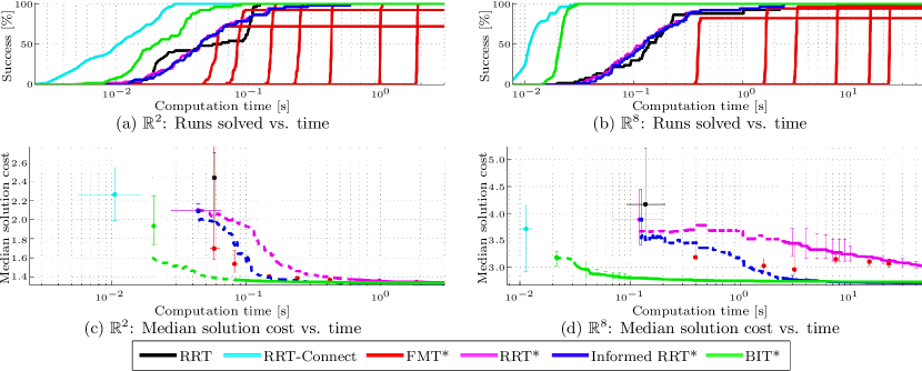
Figure 5: The results from representative worlds in $\mathbb{R}^{2}$ and $\mathbb{R}^{8}$ for RRT, RRT-Connect, RRT*, Informed RRT*, BIT* with a batch size of $100$ samples, and FMT* of various sample sizes ($\mathbb{R}^{2}$: $500$, $1000$, $2500$, $5000$, $10000$, $25000$, and $50000$; $\mathbb{R}^{8}$: $100$, $500$, $1000$, $2500$, $5000$, and $7500$). For the chosen random worlds, (a) and (b) show the percentage of trials solved versus run time for the $50$ different trials, while (c) and (d) show the median solution cost versus run time. Dots represent the median initial solution. For algorithms that asymptotically converge towards the optimum, the dashed lines represent a median calculated from $50\%$–$100\%$ success rate and may increase as new trials are included. The solid lines represent the median when all trials have a solution, with error bars denote a non-parametric $95\%$ confidence interval on median solution cost and time. Note that for some algorithms the confidence intervals are smaller than the median line and are not visible and that RRT and RRT-Connect are not asymptotically optimal planners.

IV Analysis

For brevity, we only present a proof of almost sure asymptotic optimality (Theorem 1) and note that this implies probabilistic completeness. We also present a discussion on the relationship between BIT*’s edge queue and LPA*’s vertex queue (Remark 1).

Theorem 1 (Asymptotic Optimality)

BIT* asymptotically converges almost surely to the optimal solution to Prob. 1, if a solution exists, as the total number of samples, $q$, goes to infinity, i.e.,

$$\textstyle P\left(\limsup\limits_{q\to\infty}c_{{\rm best},q}^{\rm\scriptscriptstyle BIT*}=s^{*}\right)=1,$$

where $c_{{\rm best},q}^{\rm\scriptscriptstyle BIT*}$ is the cost of the best solution found by BIT* from $q$ samples.

Proof:

The proof extends directly from the work in [23]. In Appendix G, Karaman and Frazzoli show that for $q$ uniformly distributed random samples and a specific constant $r_{q}$, the solution found by RRT* almost surely converges asymptotically to the optimal solution as $q$ goes to infinity, i.e.,

$$\textstyle P\left(\limsup\limits_{q\to\infty}c_{{\rm best},q}^{\rm\scriptscriptstyle RRT*}=s^{*}\right)=1.$$

RRT* processes the sequence of $q$ samples individually. For any sample, it considers all edges involving samples earlier in the sequence that are less than length $r_{q}$. BIT* processes the sequence of samples in batches. For any sample in a batch, it considers all edges involving samples from the same or earlier batches that are less than length $r_{q}$. This will contain all the edges considered by RRT* for the same sequence and $r_{q}$. As BIT* maintains uniform sample density in the subproblem that contains all better solutions and (1) meets the requirements for almost sure asymptotic optimality given in [23], BIT* is almost surely asymptotically optimal. ∎

Remark 1 (Equivalence to LPA* vertex queue)

BIT*’s edge queue is an extension of LPA*’s vertex queue [17] to include a heuristic estimate of edge cost.

Explanation: LPA* uses a queue of vertices ordered lexicographically first on the solution cost constrained to go through the vertex and then the cost-to-come to the vertex. Both these terms are calculated for a vertex, $\mathbf{v}\in V$, considering all the incoming edges (rhs-value in LPA*), i.e.,

$$\textstyle\min\limits_{\left(\mathbf{u},\mathbf{v}\right)\in E}\left\{g_{\mathcal{T}}\left(\mathbf{u}\right)+c\left(\mathbf{u},\mathbf{v}\right)\right\},$$ (2)

where $E$ is the set of edges.

This minimum requires the calculation of the true edge cost between a vertex and all of its possible parents. This calculation is expensive in sampling-based planning (e.g., collision checking, differential constraints, etc.), and reducing its calculation is desirable. This can be done by using an admissible heuristic estimate of edge cost and calculating (2) incrementally. A running minimum is calculated by processing edges in order of increasing estimated cost. The process finishes, and the true minimum is found, when the estimated cost through the next edge is higher than the current value.

BIT* combines these individual minima calculations into a single edge queue. In doing so, it simultaneously calculates the minimum cost-to-come for each vertex while expanding vertices in order of increasing estimated solution cost. ∎

V Experimental Results

BIT* was tested against existing algorithms in both simulated random worlds (Section V-A) and real-world manipulation problems (Section V-B) using publicly available Open Motion Planning Library (OMPL) [38] implementations. All tests and algorithms used an RGG constant (e.g., $\eta$ in (1)) of $1.1$ and approximated $\lambda\left(X_{\rm free}\right)$ with $\lambda\left(X\right)$. RRT-based algorithms used a goal bias of $5\%$. BIT* used $100$ samples per batch, Euclidean distance between states for heuristics, and direct informed sampling [28]. Graph pruning was limited to changes in the solution cost greater than $1\%$ and we used an approximately sorted queue.

V-A Simulated Random Worlds

BIT* was compared to existing sampling-based algorithms on random problems minimizing path length in $\mathbb{R}^{2}$ and $\mathbb{R}^{8}$. The problems consisted of a (hyper)cube of width $2$ populated with random axis-aligned (hyper)rectangular obstacles such that at most one third of the environment was obstructed. The initial state was in the centre of the world and the goal was $(0.9,0.9,\ldots,0.9)$ away (Fig. 4). BIT* was compared to the OMPL implementations of RRT, RRT-Connect [39], RRT*, Informed RRT*, and FMT*. The RRT-based planners used a maximum edge length of $0.2$ and $1.25$ in $\mathbb{R}^{2}$ and $\mathbb{R}^{8}$, respectively. All algorithm parameters were chosen in good faith to maximize performance on a separate training set of random worlds.

For each state dimension, $10$ different random worlds were generated and the planners were tested with $50$ different pseudo-random seeds on each. The solution cost of each planner was recorded every $1$ millisecond by a separate thread. For each world, median solution cost was calculated for a planner by interpolating each trial at a period of $1$ millisecond. As the true optima for these problems are different and unknown, there is no meaningful way to compare the results across problems. Instead, results from a representative problem are presented in Fig. 5, where the percent of trials solved and the median solution cost are plotted versus computational time.

These experiments show that in both $\mathbb{R}^{2}$ (Figs. 5a, 5c) and $\mathbb{R}^{8}$ (Figs. 5b, 5d), BIT* generally finds better solutions faster than other sampling-based optimal planners and RRT. It has a higher likelihood of having found a solution at a given computational time than these planners, and converges faster towards the optimum. The only planner tested that found solutions faster than BIT* was RRT-Connect, a nonasymptotically optimal planner.

V-B Motion Planning for Manipulation

To evaluate the performance of BIT* on real-world high-dimensional problems, it was tested on HERB [33]. Experiments consisted of both dual-arm and one-arm planning problems for manipulation with a goal of minimizing the path length through configuration space. Parameter values for BIT* and RRT-based planners were chosen from the results of Section V-A, and the number of FMT* samples was chosen to use the majority of the available computational time. Once again, BIT* outperformed all planners other than RRT-Connect.

For the dual-arm planning problem, HERB started with both arms extended under a table from the elbow onward. The task was to plan a trajectory for both arms to place the hands in position to open a bottle (Fig. 1). HERB’s proximity to the table and starting position created a narrow passage for the arms around the table. Coupled with the $14$- degree-of-freedom (DOF) configuration space, this made for a challenging problem.

Given $2.5$ minutes of planning time, BIT* was almost twice as likely to find a solution than RRT, Informed RRT*, or FMT*. Over $25$ trials, BIT* was $68\%$ successful with a median solution cost of $17.4$. RRT-Connect was $100\%$ successful, but had a median solution cost of $22.1$. RRT was $8\%$ successful with a median solution cost of $31.1$ and Informed RRT* was $8\%$ successful with a median solution cost of $25.3$. FMT* with $m=500$ was $36\%$ successful with a median solution cost of $17.2$. All RRT-based planners used a maximum edge length of $3$.

An easier one-arm planning problem was also tested. HERB started with its left arm folded at the elbow and held at approximately the table level of a table. The task was to plan a trajectory to place the left hand in position to grasp a box (Fig. 6). The smaller configuration space, $7$ DOF, and a starting position partially clear of the table made this an easier planning problem. In the given $5$ seconds of computational time, both BIT* and RRT-Connect found a solution in all $25$ trials. BIT* had a median solution cost of $6.8$ while RRT-Connect had a median solution cost of $10.6$. RRT was $88\%$ successful with a median solution cost of $11.2$ and Informed RRT* was $88\%$ successful with a median solution cost of $10.6$. FMT* with $m=50$ was $52\%$ successful with a median solution cost of $9.0$. All RRT-based planners used a a maximum edge length of $1.25$.

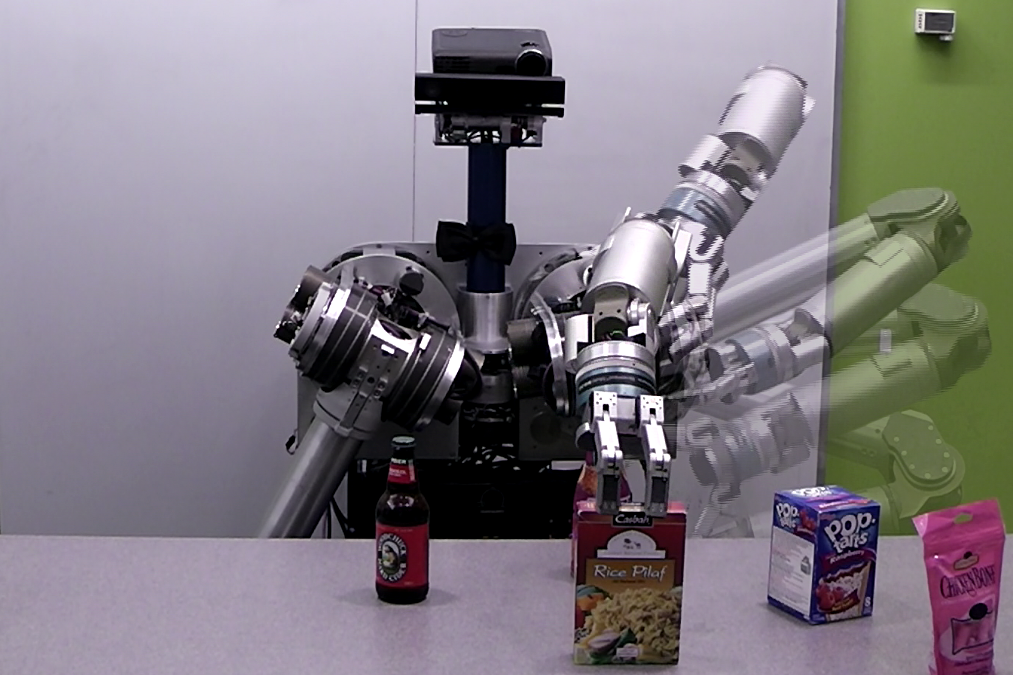
Figure 6: A composite figure of a one-arm trajectory on HERB found by BIT*. Over $25$ trials with $5$ seconds of computational time, BIT* had a median solution cost of $6.8$ and success rate of $100\%$, while Informed RRT* and FMT* had median costs of $10.6$ and $9.0$ and success rates of $88\%$ and $52\%$, respectively. Nonoptimal planners, RRT and RRT-Connect, had median costs of $11.2$ and $10.6$ and success rates of $88\%$ and $100\%$, respectively.

VI Discussion & Future Work

BIT* demonstrates that anytime sampling-based planners can be designed by combining incremental graph-search techniques with RGG theory. We hope that this work will motivate further unification of these two planning paradigms.

A fundamental component of BIT* is the application of heuristic estimates to all aspects of path cost. Doing so allows the algorithm to account for future graph improvements (cost-to-come), avoid unnecessary collision checks and boundary-value problems (edge cost), and order and focus the search (solution cost). As always, the benefit of these heuristics will depend on their suitability for the specific problem, but we feel that they are an important tool to reduce the curse of dimensionality. Note that while direct sampling of the subproblem is possible for some cost functions [28], rejection sampling is applicable. Also note that, as with other heuristically guided searches (e.g., A*), BIT* works with the trivial zero heuristic (e.g., Dijkstra’s algorithm); however, more conservative heuristics provide less benefit to the search.

In describing BIT* as an extension of LPA* to continuous planning problems, it is important to note a key difference in how they reuse information. In LPA*, updating the cost-to-come of a vertex requires reconsidering the cost-to-come of all possibly descendent vertices. This is a step that becomes prohibitively expensive in anytime resolution planners as graph size increases quickly. The results of RRT* demonstrate that this is unnecessary for the planner to almost surely converge asymptotically to the optimum as the number of samples approaches infinity.

While the efficiency of graph-search techniques is well understood, this area remains understudied for sampling-based planners. We are actively investigating whether BIT*’s use of graph-search techniques and RGG theory can be used to probabilistically evaluate its efficiency.

Also of interest are possible improvements to BIT*, including the fact that BIT* does not remove samples when connection attempts fail. This is a requirement of the uniform sample distribution used in RGG theory, but leaves edges in the implicit RGG that are known to be unusable.

Finding an efficient method to avoid these edges would improve BIT*, and there are multiple potential ways to accomplish this. Failed edges could be tracked and prevented from reentering the queue, but initial attempts have proven too computational expensive. Samples that fail multiple connection attempts could be removed, but doing so will require RGG theory for nonuniform distributions. Our current focus is on the adaptively varying batch size to increase the rate at which these edges are removed from the RGG.

We are also interested in more general extensions to BIT*. Its expanding search is well suited for large or unbounded planning problems, and we have had initial success with a version that generates samples as needed and avoids the a priori definition of state space limits. Its relationship to incremental search techniques also suggests it may be well suited for planning problems in changing environments. We are also investigating the use of other graph-search techniques, including anytime [14, 15, 16] or bidirectional [40, 41] searches to decrease the time required to find an initial solution. Finally, we are investigating combining BIT*’s global search with local searches, such as path-smoothing.

VII Conclusion

In this paper, we attempt to unify graph-search and sampling-based planning techniques through RGG theory. By recognizing that a set of samples defines an implicit RGG and using incremental-search techniques, we are able to combine the efficient search of algorithms such as A*, with the anytime scalability of sampling-based algorithms such as RRT*. The resulting algorithm, BIT*, uses heuristics for all aspects of path cost in order to prioritize the search of high-quality paths and focus the search for improvements.

As demonstrated on both simulated and real-world experiments, BIT* outperforms existing sampling-based optimal planners and RRT, especially in high dimensions. For a given computational time, BIT* has a higher likelihood of finding a solution and generally finds solutions of equivalent quality sooner. It also converges towards the optimum faster than other asymptotic optimal planners, and has recently been shown to perform well on problems with differential constraints [42]. Information on the OMPL implementation of BIT* is available at http://asrl.utias.utoronto.ca/code.

References

- [1] E. W. Dijkstra, “A note on two problems in connexion with graphs,” Numerische Mathematik, 1(1): 269–271, 1959.
- [2] P. E. Hart, N. J. Nilsson, and B. Raphael, “A formal basis for the heuristic determination of minimum cost paths,” TSSC, 4(2): 100–107, Jul. 1968
- [3] R. E. Bellman, “The theory of dynamic programming,” Bull. of the AMS, 60(6): 503–516, 1954.
- [4] D. P. Bertsekas, “Convergence of discretization procedures in dynamic programming,” TAC, 20(3): 415–419, Jun. 1975.
- [5] R. E. Bellman, Dynamic Programming. Princeton Uni. Press, 1957.
- [6] T. Lozano-Pérez and M. A. Wesley, “An algorithm for planning collision-free paths among polyhedral obstacles,” CACM, 22(10): 560–570, Oct. 1979.
- [7] P. C. Chen and Y. K. Hwang, “SANDROS: a motion planner with performance proportional to task difficulty,” in ICRA, 3: 2346–2353, May 1992.
- [8] C. S. Sallaberger and G. M. D’Eleuterio, “Optimal robotic path planning using dynamic programming and randomization,” Acta Astronautica, 35(2–3): 143–156, 1995.
- [9] J. Barraquand and J.-C. Latombe, “Nonholonomic multibody mobile robots: controllability and motion planning in the presence of obstacles,” in ICRA, 3: 2328–2335, Apr. 1991.
- [10] K. M. Lynch and M. T. Mason, “Stable pushing: Mechanics, controllability, and planning,” IJRR, 15(6): 533–556, 1996.
- [11] M. Cherif, “Kinodynamic motion planning for all-terrain wheeled vehicles,” in ICRA, 1: 317–322, 1999.
- [12] B. Donald, P. Xavier, J. Canny, and J. Reif, “Kinodynamic motion planning,” JACM, 40(5): 1048–1066, Nov. 1993.
- [13] K. Kondo, “Motion planning with six degrees of freedom by multistrategic bidirectional heuristic free-space enumeration,” TRA, 7(3): 267–277, Jun. 1991.
- [14] M. Likhachev, D. Ferguson, G. Gordon, A. Stentz, and S. Thrun, “Anytime dynamic A*: An anytime, replanning algorithm,” in ICAPS, Jun. 2005.
- [15] D. Ferguson and A. Stentz, “The delayed D* algorithm for efficient path replanning,” in ICRA, 2045–2050, Apr. 2005.
- [16] M. Likhachev, D. Ferguson, G. Gordon, A. Stentz, and S. Thrun, “Anytime search in dynamic graphs,” Art. Intel., 172(14): 1613–1643, 2008.
- [17] S. Koenig, M. Likhachev, and D. Furcy, “Lifelong planning A*,” Art. Intel., 155(1–2): 93–146, 2004.
- [18] A. Stentz, “The focussed D* algorithm for real-time replanning,” in IJCAI 1652–1659, 1995.
- [19] S. Koenig and M. Likhachev, “Fast replanning for navigation in unknown terrain,” TRO, 21(3): 354–363, Jun. 2005.
- [20] L. E. Kavraki, P. Švestka, J.-C. Latombe, and M. H. Overmars, “Probabilistic roadmaps for path planning in high-dimensional configuration spaces,” TRA, 12(4): 566–580, 1996.
- [21] S. M. LaValle and J. J. Kuffner Jr., “Randomized kinodynamic planning,” IJRR, 20(5): 378–400, 2001.
- [22] D. Hsu, R. Kindel, J.-C. Latombe, and S. Rock, “Randomized kinodynamic motion planning with moving obstacles,” IJRR, 21(3): 233–255, 2002.
- [23] S. Karaman and E. Frazzoli, “Sampling-based algorithms for optimal motion planning,” IJRR, 30(7): 846–894, 2011.
- [24] C. Urmson and R. Simmons, “Approaches for heuristically biasing RRT growth,” IROS, 2: 1178–1183, 2003.
- [25] D. Ferguson and A. Stentz, “Anytime RRTs,” IROS, 5369–5375, 2006.
- [26] B. Akgun and M. Stilman, “Sampling heuristics for optimal motion planning in high dimensions,” IROS, 2640–2645, 2011.
- [27] M. Otte and N. Correll, “C-FOREST: Parallel shortest path planning with superlinear speedup,” TRO, 29(3): 798–806, Jun. 2013
- [28] J. D. Gammell, S. S. Srinivasa, and T. D. Barfoot, “Informed RRT*: Optimal sampling-based path planning focused via direct sampling of an admissible ellipsoidal heuristic,” in IROS, 2997–3004, 2014.
- [29] L. Janson and M. Pavone, “Fast marching trees: a fast marching sampling-based method for optimal motion planning in many dimensions,” in ISRR, Dec. 2013.
- [30] O. Salzman and D. Halperin, “Asymptotically-optimal motion planning using lower bounds on cost,” in ICRA, 2015.
- [31] R. Diankov and J. J. Kuffner Jr., “Randomized statistical path planning,” in IROS, 2007.
- [32] S. M. Persson and I. Sharf, “Sampling-based A* algorithm for robot path-planning,” IJRR, 33(13): 1683–1798, 2014.
- [33] S. Srinivasa, D. Berenson, M. Cakmak, A. Collet Romea, M. Dogar, A. Dragan, R. A. Knepper, T. D. Niemueller, K. Strabala, J. M. Vandeweghe, and J. Ziegler, “HERB 2.0: Lessons learned from developing a mobile manipulator for the home,” Proc. IEEE, 100(8): 1–19, Jul. 2012.
- [34] M. Penrose, Random Geometric Graphs, ser. Oxford Studies in Probability, L. C. G. Rogers, Ed. Oxford Uni. Press, 5: 2003.
- [35] F. Xue and P. R. Kumar, “The number of neighbors needed for connectivity of wireless networks,” Wireless Networks, 10(2): 169–181, 2004.
- [36] E. N. Gilbert, “Random plane networks,” SIAM, 9(4): 533–543, 1961.
- [37] S. Muthukrishnan and G. Pandurangan, “The bin-covering technique for thresholding random geometric graph properties,” in SODA, 989–998, 2005.
- [38] I. A. Şucan, M. Moll, and L. E. Kavraki, “The Open Motion Planning Library,” IEEE R&A Mag., 19(4): 72–82, Dec. 2012.
- [39] J. J. Kuffner Jr. and S. M. LaValle, “RRT-Connect: An efficient approach to single-query path planning,” in ICRA, 995–1001, 2000.
- [40] I. Pohl, “Bi-directional search,” Mach. Intel., 6: 127–140, 1971.
- [41] L. Sint and D. de Champeaux, “An improved bidirectional heuristic search algorithm,” JACM, 24(2): 177–191, Apr. 1977.
- [42] C. Xie, J. van den Berg, S. Patil, and P. Abbeel, “Toward asymptotically optimal motion planning for kinodynamic systems using a two-point boundary value problem solver,” in ICRA, 2015.