Case study of approaches to finding patterns in citation networks

Abstract

Analysis of a dataset including a network of LED patents and their metadata is carried out using several methods in order to answer questions about the domain. We are interested in finding the relationship between the metadata and the network structure; for example, are central patents in the network produced by larger or smaller companies?

We begin by exploring the structure of the network without any metadata, applying known techniques in citation analysis and a simple clustering scheme. These techinques are then combined with metadata analysis to draw preliminary conclusions about the dataset.

1 Introduction

A citation network is a graph representing citations between documents such as scholarly articles or patents. Each document is represented by a node in the graph, and each citation is represented by an edge connecting the citing node to the cited node.

Earlier work in the area of citation network analysis by Garfield, Sher, and Torpie (1964) popularized the systematic use of forward citation count as a metric for scholarly influence. Hummon and Dereian (1989) defined several new metrics to track paths of influence, which were later improved by Batagelj (2003). The PageRank algorithm was introduced by Page et al. (1999). It originally powered the Google search engine, treating hypertext links as “citations” between documents on the world wide web. These are merely a select few prior works – this listing fails to exhaust even the highlights.

1.1 Case study: LED patents

In this paper, we will be using a network of roughly one hundred thousand LED patent applications supplied by Simons (2011).

All data is stored in plain latin-1-encoded text, with one row of data per line of text, and fields separated by tab characters.

Each patent application has a unique identifier: applnID.

The dataset includes a list of all citations (mapping the citing applnID to the cited applnID), in addition to several metadata fields:

• appMyName – normalized name of company applying for patent

1.1.1 A very brief history of LED patents

Partridge (1976) filed the first patent demonstrating electroluminescence from polymer films, one of the key advances that lead to the development of organic LEDs. (This is applnID 47614741 in our dataset.)

Kodak researchers VanSlyke and Tang (1985) built on this work when they filed a new patent demonstrating improved power conversion in organic electroluminescent devices. (This is applnID 51204521 in our dataset.) Another group of Kodak scientists, Tang, Chen, and Goswami (1988), patented the first organic LED device, now used in televisions, monitors, and phones.

This background helps to validate our methods for classifying patents as “important.” A good algorithm should classify the 47614741 and 51204521 nodes as significant. When we present our techniques, we will use this as one metric of success.

1.2 Computation

The computation for our analysis was performed using the Python programming language (http://python.org/) and the following libraries:

• networkx for network representation and analysis (Hagberg, Swart, and S Chult 2008)

• pandas for tabular data analysis (McKinney 2012)

• scipy for statistics (Jones et al. 2001)

• matplotlib for creating plots (Hunter 2007)

More information about the code written for this paper can be found under the section, Code.

2 Approaches

2.1 Network structure

The graph has 127,526 nodes and 327,479 edges.

2.1.1 Forward citations (indegree)

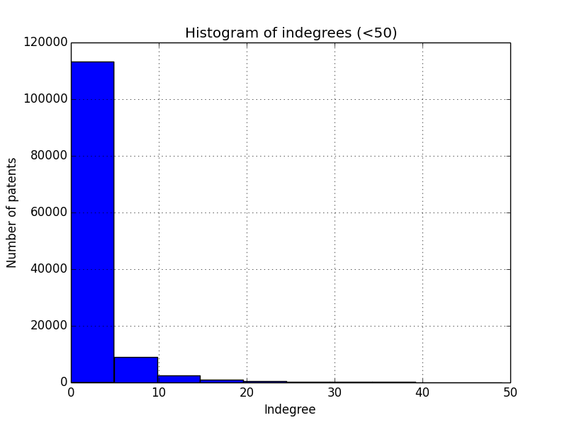
Figure 1: Histogram of patents with under 50 citations

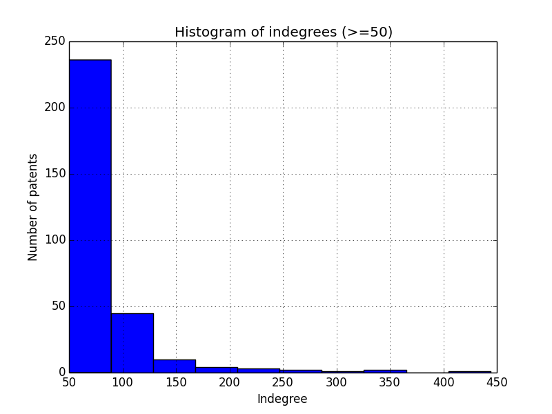
Figure 2: Histogram of patents with 50 or more citations

Popularized by Garfield, Sher, and Torpie (1964), the simplest way to determine a patent’s relative importance is counting its forward citations – that is, other patents which cite the patent in question. In a citation network where edges are drawn from the citing patent to the cited patent, the number of forward citations for a given node is its indegree, or the number of edges ending at the given node.

In our data, 89% of patents have fewer than 5 citations, and 99% have fewer than 50. Nevertheless, there is a small group of slightly over fifty patents with at least a hundred citations each.

The top ten most-cited patents in our dataset are shown in a table below:

applnID	indegree
47614741	444
51204521	360
52376694	339
48351911	305
45787627	283
45787665	267
46666643	235
53608703	213
54068562	213
23000850	203

2.1.1.1 Computation

We computed indegree using networkx.DiGraph.in_degree() (Hagberg, Swart, and S Chult 2008).

2.1.2 PageRank

Another technique for classifying important nodes in a graph is PageRank (Page et al. 1999), a famous algorithm used by the Google search engine to rank web pages.

PageRank calculates the probability that someone randomly following citations will arrive at a given patent. The damping factor $d$ represents the probability at each step that the reader will continue on to the next patent.

For each patent in our dataset, we calculated:

• pagescore – raw PageRank score (probability 0 to 1)

• page_rank – relative numerical rank of the patent (by PageRank)

• indegree – number of forward citations

• indegree_rank – relative numerical rank of the patent (by indegree)

The following chart shows the top ten patents sorted by PageRank:

applnID	pagescore	page_rank	indegree	indegree_rank
47614741	0.000371	1	444	1
51204521	0.000329	2	360	2
48351911	0.000291	3	305	4
45787627	0.000241	4	283	5
48112868	0.000227	5	63	172
45787665	0.000220	6	267	6
52376694	0.000210	7	339	3
53608703	0.000193	8	213	8
46666643	0.000173	9	235	7
47823143	0.000168	10	47	342

Within our dataset, PageRank and indegree are correlated with a Pearson product-moment coefficient of $r=.80$.

2.1.2.1 Computation

We computed PageRank using networkx.pagerank_scipy() with max_iter set to 200 and a damping factor of $d=.85$ (Page et al. 1999; Hagberg, Swart, and S Chult 2008).

2.2 Clustering

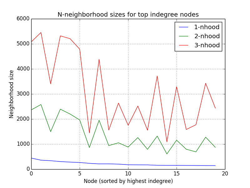
Figure 3: Neighborhood sizes for top 20 cited patents

As noted by Satuluri and Parthasarathy (2011), most clustering techniques deal with undirected graphs. We introduce a very simple technique for defining overlapping clusters in a directed citation network:

• Select a small number of highly cited patents as seeds.

• Each seed patent defines a cluster: all patents citing the seed are members (its open 1-neighborhood).

We considered using larger neighborhoods. The $n$-neighborhood can be computed recursively by adding all patents citing any patents in the $(n-1)$-neighborhood. However, these larger neighborhoods grow in size very quickly. For our purposes of quick computation and visualization, we chose to keep the smaller clusters from 1-neighborhoods.

This technique creates overlapping clusters, where a node can belong to more than one cluster. Looking at the clusters created from the top 10 most-cited patents, we computed two measures of overlapping:

• percentunique is the fraction of nodes in only that cluster

• bignodes is the number of seed nodes that appear in the cluster (for example, the second cluster contains the seed patent used to generate the first cluster, along with three others from our original ten seeds)

The following chart shows the value of percentunique and bignodes for each of the ten clusters:

clustersize	percentunique	bignodes
444	0.202703	0
360	0.100000	4
339	0.280236	0
305	0.163934	4
283	0.141343	0
267	0.101124	0
235	0.940426	0
213	0.985915	0
213	0.464789	0
203	0.226601	0

Looking at percentunique, many clusters have a good deal over overlap, with unique contributions as low as 10%, although others are up to 98% unique. Our analysis will therefore not assume that these clusters strictly partition the data, and rather look at the clusters as distinct but potentially overlapping areas of patents.

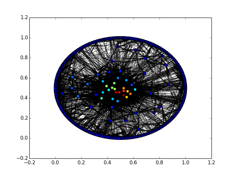
Figure 4: 1-neighborhood of applnID=47614741 (444 nodes)

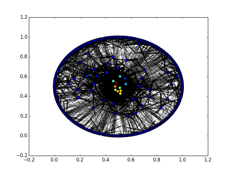
Figure 5: 1-neighborhood of applnID=45787627 (283 nodes)

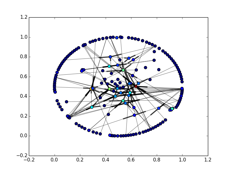
Figure 6: 1-neighborhood of applnID=23000850 (203 nodes)

2.2.0.1 Computation

The $n$-neighborhood of a node can be computed using the included code:

neighborhood(graph, nbunch, depth=1, closed=False)

• graph – a networkx.DiGraph (see Hagberg, Swart, and S Chult 2008)

• nbunch – a node or nodes in graph

• depth – the number of iterations (defaults to 1-neighborhood)

• closed – set to True if the neighborhood should include the root

Returns a set containing the neighborhood of the node, or a dict matching nodes to neighborhood sets.

2.3 Metadata analytics

Note that only about 35% of the patents in our dataset (44356 out of 127526) were supplied with appMyName (company name).

2.3.1 Choosing a metric for company size

We would like to explore whether company size has any correlation with patent quality. Do major innovations originate from big labs, or do smaller companies pave the way (only to be later acquired)?

In order to begin this investigation, we need a solid metric to quantify “company size.” Our first thought was to use a metadata-based solution, such as the company’s net worth or number of employees. However, it wasn’t clear at which point in time to measure the company size – does a company’s employee count in 2013 affect the quality of a patent it filed in the 1980s?

Instead, we choose a simple metric contained within our dataset: company size is defined as the number of patents submitted.

This may not be a perfect representation of “size,” but it still allows us to analyze whether these “prolific” companies are contributing any important patents or merely a large volume of consequential patents.

Our set of “large companies” will therefore be the 25 companies that applied for the largest number of patents. They are, in order with number of LED patents each:

samsung (1673), semiconductor energy lab (1437), seiko (1394), sharp (1103), panasonic (1094), sony (937), toshiba (848), sanyo (tokyo sanyo electric) (793), philips (789), kodak (767), hitachi (632), osram (631), nec (621), lg (613), idemitsu kosan co (553), canon (538), pioneer (525), mitsubishi (501), rohm (420), tdk (384), nichia (370), fujifilm (369), ge (363), sumitomo (323), lg/philips (293)

2.3.2 Summed outdegree

The “summed score” metric isn’t very useful in this situation, since we’ve already ranked our patents by frequency in our definition of company size. The summed score for outdegree gives us little new information.

Below is our list of top 25 patents, with their relative ranking by summed outdegree score in parentheses:

samsung (2), semiconductor energy lab (1), seiko (3), sharp (5), panasonic (6), sony (7), toshiba (8), sanyo (tokyo sanyo electric) (10), philips (9), kodak (4), hitachi (15), osram (14), nec (11), lg (17), idemitsu kosan co (12), canon (16), pioneer (13), mitsubishi (18), rohm (22), tdk (20), nichia (19), fujifilm (25), ge (21), sumitomo (26), lg/philips (27)

As expected, our top-frequency companies have very high rankings by summed outdegree score.

2.3.3 Normalized summed outdegree

Instead, we can look at the normalized outdegree, or the mean outdegree of a patent produced by one of our companies. Let’s take a look at just our top 10 companies:

1. samsung – 11.51

2. semiconductor energy lab – 14.91

3. seiko – 13.06

4. sharp – 13.39

5. panasonic – 13.13

6. sony – 13.23

7. toshiba – 14.22

8. sanyo (tokyo sanyo electric) – 13.86

9. philips – 14.47

10. kodak – 19.98

By comparison, the mean outdegree over all patents is 5.60.

2.3.4 Contribution factor – outdegree

Let us define patents as relatively significant if their outdegree is in the 75th percentile. (For our LED dataset, this includes all patents with at least 11 citations.)

Then, we can calculate contribution factors for each company by finding the fraction of their patents that are considered relatively significant. Here are the results:

1. samsung – .63

2. semiconductor energy lab – .85

3. seiko – .78

4. sharp – .86

5. panasonic – .85

6. sony – .82

7. toshiba – .89

8. sanyo (tokyo sanyo electric) – .88

9. philips – .76

10. kodak – .84

2.3.5 Date partitioning

Another interesting approach is to look at the filing date of the patents. Below is a histogram of number of patents by filing date.

date range                  count
1940-11-12 to 1945-07-06    1
1945-07-06 to 1950-02-28    6
1950-02-28 to 1954-10-23    107
1954-10-23 to 1959-06-17    247
1959-06-17 to 1964-02-09    369
1964-02-09 to 1968-10-03    344
1968-10-03 to 1973-05-28    362
1973-05-28 to 1978-01-20    575
1978-01-20 to 1982-09-14    678
1982-09-14 to 1987-05-09    1125
1987-05-09 to 1992-01-01    2257
1992-01-01 to 1996-08-25    3451
1996-08-25 to 2001-04-19    8103
2001-04-19 to 2005-12-12    16019
2005-12-12 to 2010-08-06    5040

We can partition each company’s patents into thirds – that is, samsung0 contains the first chronological third of Samsung’s patents, samsung1 contains the second third, and samsung2 contains the final third.

We can calculate normalized outdegree for each third:

company    partition  start       end         normalizedoutdeg    count  totalcount
samsung    0          1989-05-30  2004-06-28  2.6858168761220824  557    1673
samsung    1          2004-06-28  2005-11-30  1.3375224416517055  557    1673
samsung    2          2005-12-02  2010-07-13  0.5116279069767442  559    1673
sel        0          1982-02-09  2002-02-26  8.187891440501044   479    1437
sel        1          2002-02-28  2004-06-23  5.1941544885177455  479    1437
sel        2          2004-06-25  2010-01-06  1.3528183716075157  479    1437
seiko      0          1973-07-13  2002-02-22  5.644396551724138   464    1394
seiko      1          2002-02-25  2004-01-21  2.543103448275862   464    1394
seiko      2          2004-01-21  2009-06-18  0.9978540772532188  466    1394
sharp      0          1972-07-31  1994-02-22  4.809264305177112   367    1103
sharp      1          1994-02-25  2001-10-29  3.5476839237057223  367    1103
sharp      2          2001-10-31  2010-02-26  1.8130081300813008  369    1103
panasonic  0          1963-11-18  1997-10-31  3.4148351648351647  364    1094
panasonic  1          1997-11-05  2002-02-21  3.6950549450549453  364    1094
panasonic  2          2002-02-27  2010-03-05  2.2868852459016393  366    1094
sony       0          1970-04-13  2000-09-11  4.064102564102564   312    937
sony       1          2000-09-14  2003-08-20  4.0576923076923075  312    937
sony       2          2003-08-28  2010-02-10  1.5878594249201279  313    937
toshiba    0          1969-08-25  1993-03-30  4.184397163120567   282    848
toshiba    1          1993-04-13  2001-04-27  6.1063829787234045  282    848
toshiba    2          2001-04-27  2010-03-23  2.3732394366197185  284    848
sanyo      0          1976-12-09  2000-03-17  6.943181818181818   264    793
sanyo      1          2000-03-17  2003-03-28  3.25                264    793
sanyo      2          2003-03-28  2009-01-15  1.4037735849056603  265    793
philips    0          1954-01-29  1999-09-08  6.011406844106464   263    789
philips    1          1999-09-08  2004-07-01  6.068441064638783   263    789
philips    2          2004-07-09  2009-06-03  1.326996197718631   263    789
kodak      0          1965-03-25  2001-01-30  23.63529411764706   255    767
kodak      1          2001-02-02  2003-09-23  4.670588235294118   255    767
kodak      2          2003-09-24  2008-02-25  1.7042801556420233  257    767

3 Conclusions

Based on our meta-metrics, it appears that while large companies file many patent applications, these patents are not of any lower quality than average.

By the normalized summed outdegree measure, the top 10 companies each had a mean outdegree more than double that of the entire dataset.

By contribution factor analysis, each of the top 10 (except Samsung) still exceeded the expected ratio.

4 Code

The code for this paper will be posted to GitHub.

Each figure and chart was generated by a different function:

# Analysesbig_companies(graph, metadata, show_table=True)visualize_cluster(graph, index=1, show_plot=False)visualize_cluster(graph, index=5, show_plot=False)analyze_pagerank(graph, show_table=False, show_plot=False)analyze_indegree(graph, show_table=False, show_plot=False)analyze_nhood_overlap(graph, show_table=False)analyze_nhood_size(graph, show_table=False, show_plot=False)

5 References

Batagelj, Vladimir. 2003. “Efficient Algorithms for Citation Network Analysis.” ArXiv Preprint Cs/0309023.

Garfield, Eugene, Irving H. Sher, and Richard J. Torpie. 1964. “The Use of Citation Data in Writing the History of Science.” DTIC Document.

Hagberg, Aric, Pieter Swart, and Daniel S Chult. 2008. “Exploring Network Structure, Dynamics, and Function Using NetworkX.” Los Alamos National Laboratory (LANL).

Hummon, Norman P., and Patrick Dereian. 1989. “Connectivity in a Citation Network: The Development of DNA Theory.” Social Networks 11 (1): 39–63.

Hunter, J. D. 2007. “Matplotlib: A 2D Graphics Environment.” Computing In Science & Engineering 9 (3): 90–95.

Jones, Eric, Travis Oliphant, Pearu Peterson, and others. 2001. “SciPy: Open Source Scientific Tools for Python.” http://www.scipy.org/.

McKinney, Wes. 2012. Python for Data Analysis. O’Reilly Media.

Page, Lawrence, Sergey Brin, Rajeev Motwani, and Terry Winograd. 1999. “The PageRank Citation Ranking: Bringing Order to the Web.”

Partridge, Roger Hugh. 1976. “Radiation Sources.” Google Patents.

Satuluri, Venu, and Srinivasan Parthasarathy. 2011. “Symmetrizations for Clustering Directed Graphs.” In Proceedings of the 14th International Conference on Extending Database Technology, 343–354. ACM.

Simons, Kenneth. 2011. “Files with Patent Data on Technology Classifications.”

Tang, Ching W., Chin H. Chen, and Ramanuj Goswami. 1988. “Electroluminescent Device with Modified Thin Film Luminescent Zone.” Google Patents.

VanSlyke, Steven A., and Ching W. Tang. 1985. “Organic Electroluminescent Devices Having Improved Power Conversion Efficiencies.” Google Patents.