Perturbative QCD in acceptable schemes with holomorphic coupling

Abstract

Perturbative QCD in mass independent schemes leads in general to running coupling $a(Q^{2})$ which is nonanalytic (nonholomorphic) in the regime of low spacelike momenta $|Q^{2}|\lesssim 1\ {\rm GeV}^{2}$. Such (Landau) singularities are inconvenient in the following sense: evaluations of spacelike physical quantities ${\cal D}(Q^{2})$ with such a running coupling $a(\kappa Q^{2})$ ($\kappa\sim 1$) give us expressions with the same kind of singularities, while the general principles of local quantum field theory require that the mentioned physical quantities have no such singularities. In a previous work, certain classes of perturbative mass independent beta functions were found such that the resulting coupling was holomorphic. However, the resulting perturbation series showed explosive increase of coefficients already at ${\rm N}^{4}{\rm LO}$ order, as a consequence of the requirement that the theory reproduce the correct value of the $\tau$ lepton semihadronic strangeless decay ratio $r_{\tau}$. In this work we successfully extend the construction to specific classes of perturbative beta functions such that the perturbation series do not show explosive increase of coefficients, the perturbative coupling is holomorphic, and the correct value of $r_{\tau}$ is reproduced. In addition, we extract, with Borel sum rule analysis of the $V+A$ channel of the semihadronic strangeless decays of $\tau$ lepton, reasonable values of the corresponding $D=4$ and $D=6$ condensates.

I Introduction

The perturbative QCD (pQCD) calculations are usually performed in mass independent schemes, i.e., schemes in which beta function $\beta(a)$ of the running coupling (couplant) $a(Q^{2})$ ($\equiv\alpha_{s}(Q^{2})/\pi$) has expansion in powers of $a$ such that the beta expansion coefficients depend on the number of effective quark flavors $N_{f}$. When the squared momenta $q^{2}\equiv-Q^{2}$ are low, $|Q^{2}|\lesssim 1\ {\rm GeV}^{2}$, the mentioned coefficients have $N_{f}=3$. Such calculations give for the running coupling $a(Q^{2})$ a function which has, for the general spacelike momenta $Q^{2}\in\mathbb{C}\backslash(-\infty,0]$, nonholomorphic (singular) behavior in the small momentum regime $|Q^{2}|\lesssim 1\ {\rm GeV}^{2}$, and these singularities are usually called Landau ghosts (or Landau singularities). When any spacelike physical quantities ${\cal D}(Q^{2})$, such as the current correlators and structure functions, are evaluated in pQCD as (truncated) series involving such coupling $a(\kappa Q^{2})$ (where $\kappa\sim 1$ is a positive renormalization scale parameter), the resulting expressions ${\cal D}(Q^{2})_{\rm eval.}={\cal F}(a(\kappa Q^{2}))$ manifest the same type of singularities for $Q^{2}\in\mathbb{C}\backslash(-\infty,0]$ (and $|Q^{2}|\lesssim 1\ {\rm GeV}^{2}$). Such singularities of ${\cal D}(Q^{2})_{\rm eval.}$ are physically unacceptable, because ${\cal D}(Q^{2})$ must be an analytic (holomorphic) function of $Q^{2}$ in the entire complex $Q^{2}$ plane with the exception of the negative semiaxis $Q^{2}\in\mathbb{C}\backslash(-\infty,-M_{\rm thr}^{2}]$ (where the threshold mass is $M_{\rm thr}\sim 0.1$ GeV), this being a consequence of general principles of (local) quantum field theories BS ; Oehme . Even resummations of infinite number of terms in the perturbation expansion of ${\cal D}(Q^{2})$, practicable in QCD for example in the large-$\beta_{0}$ approximation, do not cure the problem of Landau ghosts [cf. comments following Eqs. (56) in Appendix A]. If we are to apply a universal running coupling $a(Q^{2})$ in the evaluation of a low-momentum quantity ${\cal D}(Q^{2})$, the analytic properties of $a(Q^{2})$ should reflect the mentioned analytic properties of ${\cal D}(Q^{2})$.

The notion of a universal running coupling $a(Q^{2})$ is intimately connected with the concept of perturbation expansion. Since perturbation theory is directly applicable only to those physical quantities or, to those circumstances (momenta, etc.), which are characterized by small coupling, originally only such coupling makes direct sense. Within QCD this is the coupling in the regime of high momenta (asymptotic freedom) where partons (quarks and gluons) do exist in the usual sense. Nevertheless, one can attribute a meaning to a universal running coupling outside the high momentum regime. One of the preconditions for the applicability of such a coupling is that the aforementioned nonanalyticity (Landau singularities) of $a(Q^{2})$, at low $|Q^{2}|\lesssim 1\ {\rm GeV}^{2}$ in the complex $Q^{2}$ plane outside the negative semiaxis, does not appear or is eliminated.

A formalism exists which extends the use of the universal running coupling to the regime $|Q|\sim 1$ GeV, namely the Operator Product Expansion (OPE) in the sense of the ITEP School (pQCD+OPE), Refs. Shifman1 ; Shifman2 . In such approach the inclusive spacelike quantities ${\cal D}(Q^{2})$, are evaluated by adding to the usual perturbation expansion of the term with the lowest dimension (leading-twist term), ${\cal F}(a(\kappa Q^{2}))$, other terms which involve vacuum expectation values (condensates) of various operators $O_{N}$ with higher dimensions $2N$, i.e., terms proportional to $\langle O_{N}\rangle/Q^{2N}$. Complete formalism which would extend the regime of applicability of this pQCD+OPE approach at present does not exist, but attempts have been made in this direction with the use of nonlocal condensates NLC .

Various independent lines of research support the existence of the concept of the running coupling $a(Q^{2})$ in low-momentum regime and suggest that it is finite and possibly holomorphic there: the Gribov-Zwanziger approach Gr1 ; Gr2 ; Gr3 ; Gr4 ; calculations involving Dyson-Schwinger equations (DSE) for gluon and ghost propagators and vertices DSE1a ; DSE1b ; DSE1c ; DSE1d ; DSE1e ; DSE2a ; DSE2b ; DSE2c ; DSE2d ; DSE2e ; DSE2f ; AHS ; stochastic quantization STQ ; functional renormalization group equations FRG1 ; FRG2 ; FRG3 ; lattice calculations latt1a ; latt1b ; latt1c ; latt1d . In addition, the finiteness of the coupling at $Q\to 0$ is suggested by specific applications StMatt1 ; StMatt2 of the Principle of Minimal Sensitivity (PMS) Stevenson ; St2a ; St2b , by models using the AdS/CFT correspondence modified by a dilaton backgound AdS1 ; AdS2 , in scenarios with larger quark flavor number $N_{f}$ SteveIRFP1 ; SteveIRFP2 , and in various other approaches such as those in Refs. Simonov1 ; Simonov2 ; BKSKKSh1 ; BKSKKSh2 ; BKSKKSh3 ; BKSKKSh4 ; BKSKKSh5 ; Deur ; Court .

The nonanalyticity of $a(Q^{2})$ in low-momentum regimes in the usual pQCD schemes was addressed in the seminal works of Shirkov, Solovtsov et al. ShS1 ; ShS2 ; MS ; Sh1Sh2a ; Sh1Sh2b , where a holomorphic version ${\mathcal{A}}^{\rm(APT)}(Q^{2})$ of the pQCD coupling $a(Q^{2})$ (in any mass independent scheme) was constructed, via a use of the Cauchy theorem and dispersion integral in which the offending (Landau) cut of $a(Q^{2})$ was eliminated and the cut of $a(Q^{2})$ for $Q^{2}<0$ was left unchanged; in a sense, this is a “minimal” analytization approach, widely referred in the literature as Analytic Perturbation Theory (APT). This approach includes the analogous construction, via dispersive integral, of the holomorphic analogs ${\mathcal{A}}_{n}^{\rm(APT)}(Q^{2})$ of the (integer) powers $a(Q^{2})^{n}$ of pQCD coupling. The formalism was later extended to the construction of APT analogs of any physical quantity KS , and of APT analogs ${\mathcal{A}}_{\nu}^{\rm(FAPT)}(Q^{2})$ of noninteger powers $a(Q^{2})^{\nu}$ ($\nu$ noninteger) in the works BMS1 ; BMS2 ; BMS3 (Fractional Analytic Perturbation Theory - FAPT). For a review of FAPT, see Refs. Bakulev1 ; Bakulev2 , and mathematical packages for numerical calculation are given in Refs. BK1 ; BK2 ; BK3 .

Since the publication of APT ShS1 ; ShS2 ; MS , several other (extended) analytic QCD models, i.e., models of holomorphic ${\mathcal{A}}(Q^{2})$, have been constructed Nest1a ; Nest1b ; Nest1c ; Nest1d ; Nest2a ; Nest2b ; Nest2c ; Webber ; CV12a ; CV12b ; Alekseev ; 1danQCD ; 2danQCD ; Shirkovmass . Analytic QCD models [(F)APT and others] and related dispersive approaches have been used in various contexts MSS1 ; MSS2a ; MSS2b ; MagrGl ; mes2a ; mes2b ; DeRafael ; MagrTau1 ; MagrTau2 ; Nest3a ; Nest3b ; Nest3c ; anOPE ; anOPE2a ; anOPE2b . For reviews of some analytic QCD models, see Refs. Prosperi ; Shirkov .

Furthermore, the higher power analogs ${\mathcal{A}}_{\nu}(Q^{2})$ of $a(Q^{2})^{\nu}$ in such general analytic QCD models are constructed by the procedures of Refs. CV12a ; CV12b (when $\nu$ is integer) and Ref. GCAK (when $\nu$ is general real).

It turns out that all these holomorphic couplings ${\mathcal{A}}(Q^{2})$ are nonperturbative, i.e., for $|Q^{2}|>\Lambda^{2}$ (where $\Lambda^{2}\sim 1\ {\rm GeV}^{2}$) they differ from the corresponding pQCD coupling $a(Q^{2})$ (i.e., $a(Q^{2})$ in the same scheme) by terms ${\mathcal{A}}(Q^{2})-a(Q^{2})\sim(\Lambda^{2}/Q^{2})^{N}$, where $N=1$ in the models of Refs. ShS1 ; ShS2 ; Nest1a ; Nest1b ; Nest1c ; Nest1d ; Nest2a ; Nest2b ; Nest2c ; CV12a ; CV12b ; Shirkovmass , $N=3,4,5$ in the models of Refs. 1danQCD ; Alekseev , Webber , and 2danQCD , respectively. However, the power terms $\Lambda^{2}/Q^{2}$, at high $|Q^{2}|$ (small $a(Q^{2})$), can be expressed as $\exp[-1/(\beta_{0}a(Q^{2}))]\sim e^{-1/a}$, which is a nonanalytic function in $a$ (around $a=0$). This implies that the analytic QCD models cannot be described by a perturbative beta function $\beta(a)\equiv da(Q^{2})/d\ln Q^{2}$, i.e., by a $\beta(a)$ function which is described at small $|a|$ fully by its Taylor expansion in powers of $a$. The function $\beta({\mathcal{A}})$ in all these analytic QCD models contains terms $\sim e^{-1/{\mathcal{A}}}$.

In this context, the following question appears naturally: does there exist a perturbative $\beta(a)$ function [$\beta(a)=-\beta_{0}a^{2}-\beta_{1}a^{3}-\beta_{2}a^{4}-\ldots$] such that the corresponding (perturbative) running coupling $a(Q^{2})$ is a holomorphic function in the complex plane $Q^{2}\in\mathbb{C}\backslash(-\infty,-M_{\rm thr}^{2}]$ (or $Q^{2}\in\mathbb{C}\backslash(-\infty,0]$)? In Refs. anpQCD1 ; anpQCD2 , an extensive attempt was made to obtain such an analytic pQCD (anpQCD). The major obstacles to such an effort turned out to be the simultaneous fulfillment of two requirements: a) $a(Q^{2})$ is holomorphic; b) the value of the best measured low-energy QCD observable $r_{\tau}=0.203\pm 0.004$ can be reproduced in this anpQCD. Here, $r_{\tau}$ is the QCD massless canonical part [$r_{\tau}=a+{\cal O}(a^{2})$] of the $(V+A)$-channel of the $\tau$ lepton strangeless semihadronic decay ratio $R_{\tau}(\Delta S=0)$, and in $r_{\tau}$ the quark mass effects have been subtracted and the chirality-conserving higher-twist effects are known to be very suppressed DDHMZ . The two requirements a) and b) have the tendency to be mutually exclusive: almost any anpQCD gives far too low value ($<0.14$) of $r_{\tau}$; if the free parameters in the considered classes of perturbative $\beta(a)$ functions are varied in such a way that the value $0.203$ of $r_{\tau}$ is approached (from below), the coupling $a(Q^{2})$ in general acquires singularities inside the plane $Q^{2}\in\mathbb{C}\backslash(-\infty,0]$ and thus ceases to be holomorphic. The problem of too low value of $r_{\tau}$ was already encountered earlier MSS2a ; MSS2b ; Geshkenbein for the analytic (and nonperturbative) QCD model APT of Refs. ShS1 ; ShS2 ; MS ; Sh1Sh2a ; Sh1Sh2b . Nonetheless, in Refs. anpQCD1 ; anpQCD2 , for specific classes of perturbative $\beta(a)$ functions with holomorphic $a(Q^{2})$, the $\beta(a)$ functions were modified/multiplied by another perturbative function $f_{\rm fact}(a)$ such that the perturbation expansion of $r_{\tau}$, including its first four (known) terms, gave the correct value $0.203$ and the analyticity of $a(Q^{2})$ was preserved. However, the price to pay was that the resulting beta function acquired in its expansion very large $\beta_{4}$ coefficient at $a^{5}$ ($\beta_{4}\sim 10^{6}$-$10^{7}$) and thus the fifth term $\sim a^{5}$ in the expansion of $r_{\tau}$ became uncontrollably high.

In this work we return to this problem and find an attractive solution to the mentioned problem, by constructing such perturbative ${\cal F}_{\rm fact}(a)$ functions that give perturbative beta functions $\beta(a)\propto{\cal F}_{\rm fact}(a)$ that simultaneously: (a) keep the perturbation expansion coefficients under control to an arbitrarily high order; (b) reproduce the correct value $r_{\tau}=0.203$; (c) preserve the analyticity of $a(Q^{2})$ in $Q^{2}\in\mathbb{C}\backslash(-\infty,-M_{\rm thr}^{2}]$. In Sec. II we present the formalism of integration of the renormalization group equation in the complex $Q^{2}$ plane and various conditions (analyticity, universality) that have to to be fulfilled. In Sec. III we reproduce several classes of $\beta$ functions that give holomorphic $a(Q^{2})$ but fail to achieve the value of $r_{\tau}=0.203$. In Sec. IV we introduce the functions ${\cal F}_{\rm fact}(a)$ with which we modify/multiply the beta functions of the previous Section and which give us the acceptable perturbative analytic QCD framework: holomorphic $a(Q^{2})$, the correct value $r_{\tau}=0.203$, and the perturbation expansion coefficients under control. In Sec. V we perform, with one of the obtained perturbative analytic QCD schemes, an analysis with Borel sum rules of the $V+A$ channel of the semihadronic decays of $\tau$ lepton and extract reasonable values of the corresponding $D=4$ and $D=6$ condensates. In Sec. VI we summarize our results.

II Conditions, integration

The running coupling $a(Q^{2})\equiv\alpha_{s}(Q^{2})/\pi$ in QCD fulfills the renormalization group equation (RGE)

$$Q^{2}\frac{da(Q^{2})}{dQ^{2}}=\beta\left(a(Q^{2})\right)\ ,$$ (1)

where $\beta(a)$ is beta function. In the approach of the construction of the perturbative and holomorphic coupling $a(Q^{2})={\mathcal{A}}(Q^{2})$ here, the starting point will be the construction of beta function $\beta(a)$, and then the coupling function $a(Q^{2})$ will be obtained by numerical integration of the RGE (1) in the complex $Q^{2}$ plane. We will impose three central requirements on $\beta(a)$ and the resulting $a(Q^{2})$ functions:

1. The coupling $a(Q^{2})$ is a perturbative (pQCD coupling); this is equivalent to the requirement that beta function is a holomorphic (analytic) function of $a$ at $a=0$

   $$\beta(a)=-\beta_{0}a^{2}-\beta_{1}a^{3}-\beta_{2}a^{4}-\dots=-\beta_{0}a^{2}(1+c_{1}a+c_{2}a^{2}+\ldots)\ ,$$ (2)

   cf. Refs. anpQCD1 ; anpQCD2 ; Raczka1 ; Raczka2 ; Raczka3 . For example, $\beta(a)$ cannot contain the typically nonperturbative terms $\sim\exp[-C/a(Q^{2})]$ for which the Taylor expansion around $a=0$ is blind.

2. The coupling $a(Q^{2})$ must reproduce the correct measured value $r_{\tau}=0.203\pm 0.004$, where $r_{\tau}$ is the QCD massless canonical part [$r_{\tau}=a+{\cal O}(a^{2})$] of $\tau$ lepton strangeless semihadronic decay ratio $R_{\tau}(\Delta S=0)$ (with the quark mass effects subtracted and the higher-twist effects suppressed). We recall that $r_{\tau}$ is at the moment the best measured inclusive low-energy QCD observable.

3. The coupling $a(Q^{2})$, constructed by the integration of the RGE (1), must be a holomorphic function, i.e., holomorphic in the complex $Q^{2}$ plane $Q^{2}\in\mathbb{C}\backslash(-\infty,-M_{\rm thr}^{2}]$, where the threshold mass is $M_{\rm thr}\sim 0.1$ GeV.

In the integration of Eq. (1), we first need the initial condition $a(Q^{2}_{\rm in})$ at an initial (low) scale $Q^{2}_{\rm in}$. Since we are interested in the holomorphic behavior of $a(Q^{2})$ at not very high $|Q^{2}|$ ($|Q^{2}|\lesssim(3m_{c})^{2}$), we consider for simplicity the heavy quarks $c,b,t$ to be decoupled, and the three light quarks $u,d,s$ we will consider to be massless. Stated otherwise, the number of active flavors in the RGE (1) is $N_{f}=3$. We choose our initial scale to be $Q^{2}_{\rm in}=(3m_{c})^{2}\approx 14.52\ {\rm GeV}^{2}$. In order to obtain the value of $a(Q^{2}_{\rm in})$, i.e., in the scheme determined by the considered beta function $\beta(a)$, we should first obtain the value ${\overline{a}}(Q^{2}_{\rm in})$ in the $\overline{\rm MS}$ scheme. For this, we take the present world average PDG2012 ${\overline{a}}(M_{Z}^{2})=0.1184/\pi$ and RGE-run it down by the known 4-loop $\overline{\rm MS}$ beta function ${\overline{\beta}}(a)$ from $Q^{2}=M_{Z}^{2}$ to $Q^{2}_{\rm in}=(3m_{c})^{2}$. The quark thresholds are taken at $Q_{\rm thr}=\kappa{\overline{m}}_{b}$ and $Q_{\rm thr}=\kappa{\overline{m}}_{c}$, according to the 3-loop matching conditions CKS , where $1\leq\kappa\sim 1$ and we take $\kappa=3$, and the $\overline{\rm MS}$ masses ${\overline{m}}_{b}=4.20$ GeV and ${\overline{m}}_{c}=1.27$ GeV. This gives us ${\overline{a}}(Q^{2}_{\rm in})\approx 0.0716$ (at $N_{f}=3$). The corresponding value of $a(Q^{2}_{\rm in})$ is then obtained by using the integrated form of RGE (i.e., implicit solution) in its subtracted form, cf. Appendix A of Ref. Stevenson (cf. also Appendix A of Ref. CK )

$$\frac{1}{a}+c_{1}\ln\left(\frac{c_{1}a}{1\!+\!c_{1}a}\right)+\int_{0}^{a}dx\left[\frac{\beta(x)+\beta_{0}x^{2}(1\!+\!c_{1}x)}{x^{2}(1\!+\!c_{1}x)\beta(x)}\right]$$ (3)

$$=\frac{1}{{\overline{a}}}+c_{1}\ln\left(\frac{c_{1}{\overline{a}}}{1\!+\!c_{1}{\overline{a}}}\right)+\int_{0}^{\overline{a}}dx\left[\frac{{\overline{\beta}}(x)+\beta_{0}x^{2}(1\!+\!c_{1}x)}{x^{2}(1\!+\!c_{1}x){\overline{\beta}}(x)}\right],$$

where $a\equiv a(Q^{2}_{\rm in})=a_{\rm in}$ and ${\overline{a}}\equiv{\overline{a}}(Q^{2}_{\rm in})\approx 0.0716$. We note that $\beta_{0}=(1/4)(11-2N_{f}/3)$ and $c_{1}=\beta_{1}/\beta_{0}=(1/4)(102-38N_{f}/3)/(11-2N_{f}/3)$ are the universal beta-function coefficients in the mass independent schemes ($\beta_{0}=9/4$ and $c_{1}=16/9$ for $N_{f}=3$), while the other expansion coefficients $c_{j}\equiv\beta_{j}/\beta_{0}$ ($j\geq 2$) in Eq. (2) characterize the scheme Stevenson . Any choice of $\beta$ function then determines, via Eq. (3), the initial value $a(Q^{2}_{\rm in})=a_{\rm in}$ for the numerical integration of Eq. (1).

As mentioned, the RGE (1) will be solved numerically not just for $Q^{2}>0$, but in the entire complex $Q^{2}$ plane. Following the presentation in Refs. anpQCD1 ; anpQCD2 , a new complex variable is introduced: $z=\ln(Q^{2}/Q^{2}_{\rm in})$. Then the first sheet of the complex $Q^{2}$ plane corresponds to the semiopen stripe $-\pi\leq{\rm Im}z<+\pi$ in the complex $z$ plane. The general spacelike regime $Q^{2}\in\mathbb{C}\backslash(-\infty,0]$, where $a(Q^{2})$ is holomorphic in the considered perturbative analytic QCD (anpQCD) scenarios, is represented by the open stripe $-\pi<{\rm Im}(z)<+\pi$ in the $z$-plane. The timelike (Minkowskian) semiaxis $Q^{2}\leq 0$ corresponds to the border line ${\rm Im}z=-\pi$ of the $z$-stripe. The point $Q^{2}=0$ is $z=-\infty$, and $Q^{2}=Q^{2}_{\rm in}$ ($\approx 14.52\ {\rm GeV}^{2}$) is $z=0$. In Figs. 1 (a) and (b) we present the corresponding general spacelike and timelike regimes in the complex $Q^{2}$ plane and on the $z$ stripe, respectively, with a view that $a(Q^{2})$ is holomorphic in the extended regime $Q^{2}\in\mathbb{C}\backslash(-\infty,-M_{\rm thr}^{2}]$ (where $0\leq M_{\rm thr}\lesssim 0.1$ GeV).

Figure 1: (a) Complex $Q^{2}$ plane; (b) complex $z$ plane where $z=\ln(Q^{2}/Q^{2}_{\rm in})$; the non-timelike stripe is $-\pi\leq{\rm Im}z<+\pi$.

Let us denote $a(Q^{2})\equiv F(z)$. Then RGE (1) acquires the form

$$\frac{dF(z)}{dz}=\beta(F(z))\qquad\left(F(z)\equiv a(Q^{2})\right)$$ (4)

in terms of $z=\ln(Q^{2}/Q^{2}_{\rm in})$ in the semiopen stripe $-\pi\leq{\rm Im}z<+\pi$. The requirement that $a(Q^{2})$ be holomorphic for $Q^{2}\in\mathbb{C}\backslash(-\infty,0]$ now means that $F(z)$ is holomorphic ($\Rightarrow\partial F/\partial{\overline{z}}=0$) in the open stripe $-\pi<{\rm Im}(z)<+\pi$. The (physical) singularities can appear only on the timelike line ${\rm Im}(z)=-\pi$. Let us denote $z=x+iy$ and $F=u+iv$; then we can rewrite RGE (4) as a coupled system of real partial differential equations for $u(x,y)$ and $v(x,y)$

$$\frac{\partial u(x,y)}{\partial x} = {\rm Re}\beta(u+iv)\ ,\quad\frac{\partial v(x,y)}{\partial x}={\rm Im}\beta(u+iv)\ ,$$ (5a)

$$\frac{\partial u(x,y)}{\partial y} = -{\rm Im}\beta(u+iv)\ ,\quad\frac{\partial v(x,y)}{\partial y}={\rm Re}\beta(u+iv)\ .$$ (5b)

We recall that $x=\ln(|Q^{2}|/Q^{2}_{\rm in})$, $y={\rm arg}(Q^{2})$ ($-\pi\leq y<\pi$), $u={\rm Re}\;a$, $v={\rm Im}\;a$. Having chosen an Ansatz for beta function $\beta(a(Q^{2}))\equiv\beta(F(z))$ and the corresponding initial condition value $a(Q^{2}_{\rm in})$, the integration of equations (5) is then implemented numerically to high precision by the MATHEMATICA software Math . Numerical analyses suggest that it is very difficult to obtain in this way analytic coupling $a(Q^{2})$ for $Q^{2}\in\mathbb{C}\backslash(-\infty,0]$, i.e., analytic $F(z)$ in the entire open stripe $-\pi<{\rm Im}z<\pi$, unless we require in addition also analyticity in and around the point $Q^{2}=0$ ($z=-\infty$). Stated otherwise, with certain classes of pQCD $\beta$-functions we obtain the correct holomorphic behavior of $a(Q^{2})$. We represent the analyticity in $Q^{2}$ at $Q^{2}=0$ in the form

$$a(Q^{2})=a_{0}+a_{1}(Q^{2}/\Lambda^{2})+{\cal O}[(Q^{2}/\Lambda^{2})^{2}]\ ,$$ (6)

where $a_{0}=a(Q^{2}=0)=F(z=-\infty)<\infty$, and $a_{1}\not=0$. Applying the derivative $d/dz=d/d\ln Q^{2}$ to this series, the condition reads

$$\beta^{\prime}(F)|_{F=a_{0}}=+1\ .$$ (7)

The Ansätze for beta function are thus taken in the form (cf. Refs. anpQCD1 ; anpQCD2 )

$$\beta(F)=-\beta_{0}F^{2}(1-Y)f(Y)|_{Y\equiv F/a_{0}}\ ,$$ (8)

where the function $f(Y)$ fulfills three conditions

$$f(Y)\ {\rm analytic\ at}\ Y=0\qquad{\rm(pQCD)}\ ,$$ (9a)

$$f(Y) = 1+(1+c_{1}a_{0})Y+{\cal O}(Y^{2})\qquad{\rm(pQCD)}\ ,$$ (9b)

$$a_{0}\beta_{0}f(1) = 1\qquad(Q^{2}=0\ {\rm analyticity})\ .$$ (9c)

The first condition says that the beta function is perturbative; the second accounts for the universality of the $c_{1}$ coefficient of the pQCD expansion (2); the third condition is the aforementioned condition of analyticity of $a(Q^{2})$ at $Q^{2}=0$, i.e., Eq. (6). Let us once more recall that the choice of a specific type of beta function corresponds to a specific renormalization scheme, characterized by the coefficients $c_{j}$ ($j\geq 2$) of the series expansion (2) of this beta function.

If $a_{1}=0$ in Eq. (6) and $f(Y)$ is any rational (Padé) function, Landau singularities appear, as argued in Ref. anpQCD2 (footnote 3 and Appendix A there); e.g., when $a(Q^{2})=a_{0}+{\cal O}((Q^{2}/\Lambda^{2})^{n})$ with $n\geq 2$, Landau poles of $F(z)$ appear at ${\rm Im}\;z=\pm\pi/n$.

The condition of analyticity at $Q^{2}=0$, i.e. Eq. (6), implies that there is a finite region of analyticity of $a(Q^{2})$ around $Q^{2}=0$, i.e., that the branching point of the cut $(-\infty,-M_{\rm thr}^{2}]$ of $a(Q^{2})$ in the complex $Q^{2}$ plane starts at a nonzero threshold energy $-M_{\rm thr}^{2}<0$. This implicitly signals that the masses of light pseudoscalar mesons $\pi$ and $K$ are nonzero, i.e., that the masses of $u$, $d$ and $s$ quarks are not strictly zero. Therefore, the condition (6) implicitly incorporates these effects, which would otherwise be very difficult to incorporate explicitly with nonzero light quark masses in the RGE. Another, more practical, reason for imposing the condition (6) lies in the fact that it turned out to be very difficult or impossible to achieve numerically analyticity of $a(Q^{2})$ in the Euclidean complex plane $Q^{2}\in\mathbb{C}\backslash(-\infty,0]$ unless the point $Q^{2}=0$ was also included as a point of analyticity of $a(Q^{2})$, Refs. anpQCD1 ; anpQCD2 .

Often in pQCD, the PMS Stevenson ; St2a ; St2b and effective charge (ECH) ECH1 ; ECH2 ; ECH3 ; KKP ; Gupta1 ; Gupta2 schemes (at $n$-loop level, $n$ finite) are constructed from a truncated perturbation series ${\cal D}_{\rm pt}(Q^{2})^{[n]}$ (i.e., including the terms up to $a^{n}$) of a considered spacelike observable ${\cal D}(Q^{2})$ in such a way that, in the PMS procedure all the terms $\sim a^{n+2}$ are consistently discarded in the derivatives $\partial{\cal D}(Q^{2})^{[n]}_{\rm PMS}/\partial{\rm RS}=0$ (where RS=$\ln\mu^{2},c_{2},c_{3},\ldots$), and in the ECH procedure all the terms $\sim a^{n+1}$ are consistently discarded in ${\cal D}(Q^{2})^{[n]}_{\rm ECH}$ (for example, cf. Refs. KataevStarshenko ). Such schemes have scheme coefficients $c_{j}$ ($j=2,\ldots,n-1$) which are independent of $Q^{2}$ of the considered observable ${\cal D}(Q^{2})$. If such (PMS or ECH) schemes give finite $a_{0}\equiv a(0)$, e.g. those with $c_{2}<0$, they in general do not result in holomorphic coupling $a(Q^{2})$, at least not at $Q^{2}=0$, because $a_{0}$ in general does not fulfill the condition (9c). If $a_{0}\beta_{0}f(1)>1$, there are Landau singularities and poles inside the $z$ stripe (cf. Appendix A of Ref. anpQCD2 ); if $a_{0}\beta_{0}f(1)<1$, it can happen that no singularities appear inside the $z$ stripe and the only point of nonanalyticity is $Q^{2}=0$; but then the value of $r_{\tau}$ is even generally much more below the experimental value $r_{\tau}=0.203$, Ref. progress .

III Beta functions and results

Among $f(Y)$ functions that satisfy the three conditions (9), only certain specific subsets, with free parameters within $f(Y)$ varying in restricted intervals, lead upon the numerical integration of RGE’s (5) to holomorphic behavior, i.e., to a holomorphic $F(z)$ in the entire open stripe $-\pi<{\rm Im}z<\pi$. However, the evaluation of the aforementioned $\tau$ lepton decay ratio $r_{\tau}$ gave us consistently values well below the experimental values $0.203\pm 0.004$, namely values below $0.15$. In Refs. anpQCD1 ; anpQCD2 , for representation of the numerical results, various Ansätze were used for the function $f(Y)$: (1) in the form of polynomials; (2) Padé’s (ratios of polynomials); (3) product of rescaled and translated functions of the type $(e^{-Y}-1)/Y$ and $Y/(e^{-Y}-1)$, respectively. As mentioned, it turned out that, while such functions did give us holomorphic $F(z)$ in the entire open stripe of $z$, they gave for $r_{\tau}$ far too low values ($<0.15$). Here we summarize some of the results of Refs. anpQCD1 ; anpQCD2 for the three mentioned cases.

1. The case of quadratic polynomial $f(Y)$

   $$f(Y)=1+r_{1}Y+r_{2}Y^{2}\ ,$$ (10)

   where the first coefficient is $r_{1}=(1+c_{1}a_{0})$ due to the condition (9b). In order to see whether the resulting running coupling $a(Q^{2})=F(z)\equiv F(x+iy)$ has or has not singularities within the physical stripe $-\pi<z<\pi$ (Landau singularities), we present in Figs. 2(a) and (b) the results for the quantity $|\beta(F(z))|$ which should manifest singularities at the same $z$ values as the singularities of $F(z)$. In the case $r_{2}=0$, Fig. 2(a) suggests that there are no Landau singularities, i.e., no singularities on the open stripe $-\pi<{\rm Im}z<\pi$, only singularitires on the timelike axis (${\rm Im}z=\pm\pi$). In the case $r_{2}<0$ ($r_{2}=-2$ taken), Fig. 2(b) clearly shows that there are Landau singularities. As argued in Ref. anpQCD2 , for $0\leq r_{2}<r_{1}^{2}/4$ there are no Landau poles. In the $r_{2}=0$ case there are no free parameters, because the apparently free parameters $r_{1}$ and $a_{0}=a(Q^{2}=0)$ are fixed by the conditions (9b)-(9c): $a_{0}=0.1901$ and $r_{1}=(1+c_{1}a_{0})=1.338$. We did not choose $r_{2}>0$ because, although the coupling is holomorphic, the resulting $r_{\tau}$ is even lower than in the $r_{2}=0$ case. We refer to the case (10) with $r_{2}=0$ as P[1/0] because $F(Y)$ is Padé ${\rm P}[1/0](Y)$ in this case.

2. The case of Padé [1/1] $f(Y)$

   $$f(Y)=\frac{(1-t_{1}Y)}{(1-u_{1}Y)}\ .$$ (11)

   We have seemingly three parameters ($t_{1}$, $u_{1}$ and $a_{0}$), but two of them are eliminated by the conditions (9b)-(9c). We can regard as the only free parameter the coefficient $u_{1}$. It turns out that for $u_{1}=-0.1$ we obtain approximately largest $r_{\tau}$ while still no Landau poles.

3. The case of $f(Y)$ being a product of rescaled and translated functions of the type $(e^{-Y}-1)/Y$ and $Y/(e^{-Y}-1)$

   $${\rm EE:}\;f(Y)=\frac{\left(\exp[-k_{1}(Y-Y_{1})]-1\right)}{[k_{1}(Y-Y_{1})]}\frac{[k_{2}(Y-Y_{2})]}{\left(\exp[-k_{2}(Y-Y_{2})]-1\right)}\times{\cal K}(k_{1},Y_{1},k_{2},Y_{2}).$$ (12)

   Here, the constant ${\cal K}$ ensures the required normalization $f(Y=0)=1$. At first sight, we have five free parameters: $a_{0}\equiv a(Q^{2}=0)$ and four parameters for translation and rescaling ($Y_{1}$, $k_{1}$, $Y_{2}$, $k_{2}$). Two of the parameters ($Y_{2}$ and $a_{0}$) are eliminated by the conditions (9b)-(9c). Further, $0<k_{1}<k_{2}$ must be fulfilled to get physically acceptable behavior. Figs. 3(a), (b) represent the numerical results for $|\beta(F(z))|$ for the following two chosen cases: (a) $Y_{1}=0.1;k_{1}=10;k_{2}=11$ ($\Rightarrow Y_{2}\approx 0.1839$); (b) $Y_{1}=1.1;k_{1}=6;k_{2}=11$ ($\Rightarrow Y_{2}\approx 0.2386$). Figs. 3 suggest that the case (a) has no Landau singularities, and that the case (b) clearly has Landau singularities. The case EE(a) is such that $a(Q^{2})$ is kept holomorphic and simultaneously the value of $r_{\tau}$ is higher than for most of other choices of EE parameters (but still not high enough, see later).

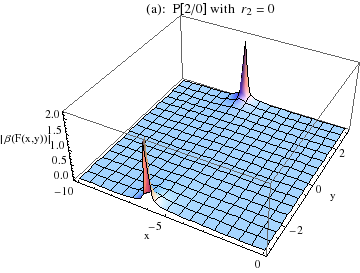
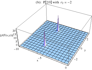
Figure 2: $|\beta(F(z))|$ as a function of $z=x+iy$ for the beta function (8) with $f(Y)$ having the form (10) with: (a) $r_{2}=0$; (b) $r_{2}=-2$.

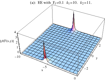
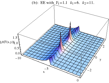
Figure 3: (a) $|\beta(F(z))|$ as a function of $z=x+iy$, where $\beta$ has the form (8) with $f(Y)$ having the “EE” form (12) with the values of free parameters $Y_{1},k_{1},k_{2}$ as indicated; (b) same as in (a), but with different values of parameters $Y_{1}$ and $k_{1}$.

In Figs. 4(a), (b) we present beta function $\beta(a)$ as a function of (positive) $a$, and in Figs. 5(a), (b) the discontinuity function $\rho_{1}(\sigma)\equiv{\rm Im}a(-\sigma-i\epsilon)$ as a function of $\ln(\sigma/Q^{2}_{\rm in})$, for two cases of holomorphic $a(Q^{2})$: for the case P[1/0] (i.e., P[2/0] with $r_{2}=0$), and for the case EE ($Y_{1}=0.1;k_{1}=10;k_{2}=11$), respectively. We note that the discontinuity function in both cases shows a clear sudden threshold jump, i.e., the cut starts at $Q^{2}=-M^{2}_{\rm thr}$, where $M_{\rm thr}=0.189$ GeV and $0.248$ GeV, respectively.

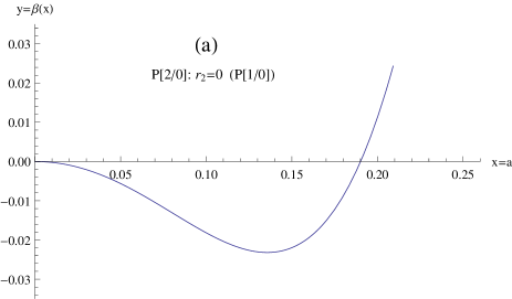
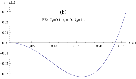
Figure 4: Beta function $\beta(a)$ as a function of positive $a$: (a) for the case when $f(Y)$ has the form (10) with $r_{2}=0$, i.e., linear polynomial; (b) for the case when $f(Y)$ is the exponential-related “EE” function (12) with $Y_{1}=0.1;k_{1}=10;k_{2}=11$.

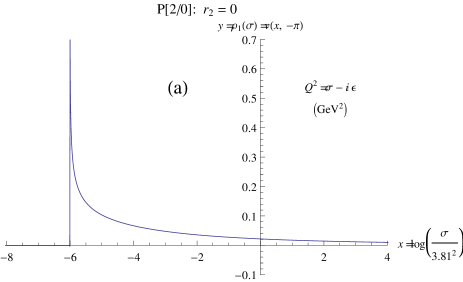
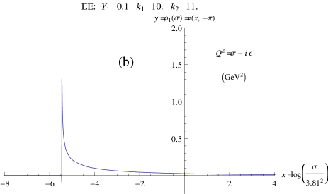
Figure 5: The discontinuity function $\rho_{1}(\sigma)={\rm Im}\ a(Q^{2}=-\sigma-i\epsilon)={\rm Im}F(z=x-i\pi)=v(x,y=-\pi)$ as a function of $x={\rm Re}(z)=\ln(\sigma/Q^{2}_{\rm in})$, for the two cases (10) and (12).

Nonetheless, the $r_{\tau}$ values, which are calculated as a leading-$\beta_{0}$ (LB) resummation plus beyond-the-leading-$\beta_{0}$ terms (bLB: NLB $\sim{\widetilde{a}}_{2}\sim a^{2}$, ${\rm N}^{2}{\rm LB}\sim{\widetilde{a}}_{3}\sim a^{3}$, ${\rm N}^{3}{\rm LB}\sim{\widetilde{a}}_{4}\sim a^{4}$), are far too low in the described cases, see Table 1. We recall that the free parameters in the three aforementioned cases (P[1/0], P[1/1], EE) were chosen in such a way as to make $r_{\tau}$ as big as possible while simultaneously preserving the holomorphic property of $a(Q^{2})$. The EE Ansatz gives us the highest $r_{\tau}\approx 0.145$, but still a long way from the experimental value $r_{\tau}=0.203\pm 0.004$.

Table 1: The four terms (and their sum) in truncated analytic expansions for $r_{\tau}$, with LB-contributions resummed and the three bLB terms organized in contour integrals of ${\widetilde{a}}_{n+1}$ [cf. Eqs. (64)-(65), with Eq. (62) and the definition (51)]. RScl parameter is $\kappa=1$ (i.e., $\mu^{2}=Q^{2}$ on the contour). Included are beta function coefficients $c_{j}$ ($j=2,3,4$), $a_{\rm in}\equiv a((3m_{c})^{2})$ and $a_{0}\equiv a(0)$ values, and the threshold mass value $M_{\rm thr}$ (in GeV).

$f$	$r_{\tau}:$ LB	NLB	${\rm N}^{2}{\rm LB}$	${\rm N}^{3}{\rm LB}$	sum	$c_{2}$	$c_{3}$	$c_{4}$	$a_{\rm in}$	$a_{0}$	$M_{\rm thr}$ [GeV]
P[1/0]	0.1122	0.0006	0.0137	0.0007	0.1272	-37.02	0	0	0.0600	0.1901	0.189
P[1/1]	0.1130	0.0006	0.0144	0.0005	0.1285	-37.54	18.84	-9.46	0.0600	0.1992	0.179
EE	0.1364	0.0009	0.0025	0.0048	0.1445	-10.80	-157.62	-644.32	0.0649	0.2360	0.248

In the Table 1 we also display the first few scheme coefficients $c_{j}$ ($j=2,3,4$), the value of $a_{0}\equiv a(0)$, and the threshold mass $M_{\rm thr}$ (in GeV).

IV Modified beta functions and results

In order to achieve the correct value $r_{\tau}=0.203$, and at the same time preserve the holomorphic behavior of $F(z)\equiv a(Q^{2})$, we follow in principle the same line of reasoning as in Sec. 3 of Ref. anpQCD1 and Sec. IV of Ref. anpQCD2 . The idea is to replace in the beta function (8)

$$f(Y)\mapsto f(Y)f_{\rm fact}(Y)\ .$$ (13)

Here, $f_{\rm fact}(Y)$ should be close to unity for the relevant values $Y\equiv a/a_{0}\equiv F(z)/a_{0}$, i.e., for the values $Y$ around the interval $(0,1)$ in the complex $Y$-plane, in order to obtain similar results for $F(z)$ as in the case without an additional factor $f_{\rm fact}(Y)$. This way there is a high probability that the coupling $F(z)$ for the replaced (modified) beta function remains holomorphic (in the entire open stripe $-\pi<{\rm Im}z<+\pi$). We note that now the conditions (9) are applied to $f_{\rm new}(Y)\equiv f(Y)f_{\rm fact}(Y)$.

One of the consequences of this condition is that the LB part of $r_{\tau}$ [cf. Eq. (62)] does not change much by this replacement, and neither do the contour integrals $I({\widetilde{a}}_{n+1})$ of the ${\rm N}^{n}{\rm LB}$ contribution [cf. Eqs. (64)-(65) and (51)]. The coefficient $T_{1}=1/12$ of the NLB contribution remains scheme independent (and small), and therefore also the NLB contribution does not change much (and remains small) under the mentioned modification. In Table 1 we can see that for the original schemes ($c_{2}^{(0)},c_{3}^{(0)},\ldots$), as defined by the beta functions Eqs. (8) and (10)-(12) [cf. also Eq. (2)], the ${\rm N}^{2}{\rm LB}$ and ${\rm N}^{3}{\rm LB}$ contributions are too small for achieving the correct value $r_{\tau}=0.203$. However, the coefficient $T_{2}$ of the ${\rm N}^{2}{\rm LB}$ contribution depends strongly on the leading scheme parameter $c_{2}$, it changes linearly with $c_{2}$ scheme coefficient of the beta function [cf. Eq. (2)]: $T_{2}(c_{2})=T_{2}(c_{2}^{(0)})-(c_{2}-{\overline{c}}_{2}^{(0)})$. The idea is then to introduce in the beta function such $f_{\rm fact}(Y)$ which fulfills simultaneously the following two conditions:

• $f_{\rm fact}(Y)\approx 1$ in the sector of the $Y$ complex plane around the $(0,1)$ interval;

• it decreases the value of $c_{2}$ to significantly lower values (from $c_{2}^{(0)}\sim-10^{1}$ of Table 1 to $c_{2}\sim-10^{2}$).

The latter condition increases the $T_{2}$ coefficient and the ${\rm N}^{2}{\rm LO}$ by about one order of magnitude and thus allows us to obtain the correct value $r_{\tau}=0.203$.

In Refs. anpQCD1 ; anpQCD2 , the $f_{\rm fact}(Y)$ functions which fulfilled the two mentioned conditions were chosen essentially in the following form:

$$f_{\rm fact}(Y)=1-\frac{K}{B}\left(\frac{BY^{2}}{1+BY^{2}}\right)\ ,$$ (14)

where $K\sim 10^{1}$ was needed to obtain $c_{2}\sim-10^{2}$ and thus the correct $r_{\tau}=0.203$, and $B\gg K$ ($B\sim 10^{3}$) was needed to keep $f_{\rm fact}(Y)\approx 1$ in the $Y$ complex plane around the $(0,1)$ interval. In this way, the sum of the first four terms, i.e., LB and ${\rm N}^{n}{\rm LB}$ ($n=1,2,3$) contributions whose coefficients $T_{n}$ are exactly known, gave the correct value $r_{\tau}=0.203$. However, the next term (${\rm N}^{4}{\rm LB}$) was then uncontrollably large: $|r_{\tau}({\rm N}^{4}{\rm LB})|\propto T_{4}\sim c_{4}\sim BK\sim 10^{6}$-$10^{7}$. This took place due to the fact that the expansion of $f_{\rm fact}(Y)$ in powers of $Y^{2}$ has a huge coefficient $BK$ at $Y^{4}$ ($(a/a_{0})^{4}$)

$$f_{\rm fact}(Y)_{\rm exp}=1-KY^{2}+(BK)Y^{4}-(B^{2}K)Y^{6}+\cdots$$ (15)

Within the present work we try to avoid this unwanted behavior in the following way: we modify the expression (14) for $f_{\rm fact}$ into an expression ${\cal F}_{\rm fact}$ such that the offending coefficients in the expansion (15) disappear

$$f_{\rm fact}(Y) \mapsto {\cal F}_{\rm fact}(Y)\ ,$$ (16a)

$${\rm such\;that}\;\;\;\;f_{\rm fact}(Y)_{\rm exp} \mapsto {\cal F}_{\rm fact}(Y)_{\rm exp}=1-KY^{2}+{\cal O}\left((Y^{2})^{P+1}\right)\ ,$$ (16b)

where the subscript “exp” denotes the expanded form of the corresponding function, $P$ is a large chosen integer, $K\sim 10^{1}$ as required by the mentioned condition (b), and at the same time requiring that the condition (a) survives: ${\cal F}_{\rm fact}(Y)\approx 1$ in the sector of the $Y$ complex plane around the $(0,1)$ interval, in order to preserve analyticity of $F(z)$. It turns out that such a transformation is possible [Eqs. (21)-(22)], as we show in the following. Let $g(\omega)$ be a function whose expansion around $\omega=0$ is

$$g(\omega)_{\rm exp}={\cal C}_{1}\omega+{\cal C}_{2}\omega^{2}+\ldots\ .$$ (17)

Consider the finite group of rotations of the complex plane given by

$$\omega\mapsto\exp\left(i\dfrac{2\pi}{P}k\right)\omega\quad\text{for }k=0,...,P-1.$$

Now consider the average of the images of $h(\omega)\equiv g(\omega)/\omega$ under this group of rotations of order $P$. We denote this average by $\widetilde{h}_{P}(\omega)\equiv\widetilde{g}_{P}(\omega)/\omega$:

$$\frac{{\widetilde{g}}_{P}(\omega)}{\omega}\equiv{\widetilde{h}}_{P}(\omega)=\frac{1}{P}\sum_{k=0}^{P-1}h(\exp\left(i\dfrac{2\pi}{P}k\right)\omega)\ .$$ (18)

It is straightforward to verify that all the terms with exponents that are not divisible by $P$ are annihilated. We are left with

$${\widetilde{g}}_{P}(\omega)_{\rm exp}={\cal C}_{1}\omega+{\cal C}_{P+1}\omega^{P+1}+{\cal C}_{2P+1}\omega^{2P+1}\ldots\ ,$$ (19)

i.e., the expansion series of ${\widetilde{g}}_{P}(\omega)$ has vanishing lowest-order terms (with the exception of the linear one). When applying this approach to $g(\omega)\equiv f_{\rm fact}(Y)-1$ of Eq. (14), with $\omega=Y^{2}$, we obtain

$${\cal F}_{\rm fact}(Y) = 1-\frac{K}{B}\left(\frac{BY^{2}}{1-(-BY^{2})^{P}}\right)\ ,$$ (20)

It turns out that the condition (a) is fulfilled only when $P$ is odd: $P=2N+1$ (because for $P=2N$ beta function has a pole at small positive $Y=1/\sqrt{B}$). Consequently, we use $P=2N+1$

$${\cal F}_{\rm fact}(Y;N) = 1-\frac{K}{B}\left(\frac{BY^{2}}{1+(BY^{2})^{2N+1}}\right)$$ (21a)

$$= \frac{1+(BY^{2})^{2N+1}-KY^{2}}{1+(BY^{2})^{2N+1}}\ ,$$ (21b)

and the expansion around $Y=0$ is

$$\Rightarrow\;{\cal F}_{\rm fact}(Y;N)_{\rm exp}=1-KY^{2}+\frac{K}{B}\left[(BY^{2})^{2N+2}-(BY^{2})^{4N+3}+(BY^{2})^{6N+4}\cdots\right]\ .$$ (22)

We recall that $K\sim 10^{1}$ and $B\gg K$. The new considered beta functions are now, according to Eqs. (8)-(9), (13), (16)

$$\beta(F)=-\beta_{0}F^{2}(1-Y)f(Y){\cal F}_{\rm fact}(Y;N)\ ,$$ (23)

where $F\equiv a(Q^{2})$, $Y\equiv F/a_{0}\equiv a/a_{0}$. For $f(Y)$ we stick to the original options Eqs. (10) ($r_{2}=0$) or (11) or (12). We note that the conditions (9) are applied now to $f_{\rm new}(Y)\equiv f(Y){\cal F}_{\rm fact}(Y)$.

Here we recall once more that the physical condition of obtaining large enough value of $r_{\tau}$ ($\approx 0.203$) imposed on us: (1) the condition of having a large value $K\sim 10^{1}$ in the expansion ${\cal F}_{\rm fact}(Y;N)_{\rm exp}=1-KY^{2}+{\cal O}(Y^{3})$ with the coefficients at higher powers of $Y$ under control; (2) and simultaneously the condition ${\cal F}_{\rm fact}(Y;N)\approx 1$ in the sector of the $Y$ complex plane around the $(0,1)$ interval. Mathematically, these two conditions tend to be in general in conflict, which explains why it was so difficult to obtain a solution, such as Eqs. (21)-(22), reconciling both of them.

In Refs. anpQCD1 ; anpQCD2 only the modification with ${\cal F}_{\rm fact}(Y;N=0)$ was investigated. We now perform the numerical integration of the RGE (5) for many different $N$, as high as $N=25$, and adjust $B$ ($\sim 10^{3}$) and $K$ ($\sim 10^{1}$) so that the correct value of $r_{\tau}$ is obtained by adding the first four terms. The higher terms $r_{\tau}({\rm N}^{n}{\rm LB})$ ($n\geq 4$) are now under control, they are estimated to contribute less than 0.001. And the holomorphic behavior of $F(z)\equiv a(Q^{2})$ is preserved when $N$ increases. In Table 2 we present the results analogous to those in Table 1, but now with $f(Y)\mapsto f(Y){\cal F}_{\rm fact}(Y;N)$ for the choices $N=0$ and $N=25$, again for the three cases of $f(Y)$: Eq. (10) with $r_{2}=0$ (P[1/0]); Eq. (11) with $u_{1}=-0.1$ (P[1/1]); Eq. (12) with $Y_{1}=0.1$, $k_{1}=10.0$, $k_{2}=11.0$.

Table 2: Same as in Table 1, but now beta function is changed by the substitution $f(Y)\mapsto f(Y){\cal F}_{\rm fact}(Y;N)$, Eqs. (21)-(23), where $N=0$ and $N=25$. Included are new beta function coefficients $c_{j}$ ($j=2,3,4$), $a_{\rm in}$ and $a_{0}$ values, and the threshold mass value $M_{\rm thr}$ (in GeV).

$f$	$N$	$B$	$K$	$r_{\tau}:$ LB	NLB	${\rm N}^{2}{\rm LB}$	${\rm N}^{3}{\rm LB}$	sum	$c_{2}$	$c_{3}$	$c_{4}$	$a_{\rm in}$	$a_{0}$	$M_{\rm thr}$ [GeV]
P[1/0]	0	5000	6.8	0.1055	0.0006	0.0911	0.0058	0.2029	-224.67	-333.73	$2.59\times 10^{7}$	0.0574	0.1903	0.159
P[1/0]	25	2100	6.8	0.1054	0.0006	0.0913	0.0058	0.2030	-225.19	-334.52	6966.7	0.0574	0.1901	0.159
P[1/1]	0	4650	7.3	0.1056	0.0006	0.0910	0.0058	0.2030	-220.89	-307.36	$2.14\times 10^{7}$	0.0573	0.1994	0.149
P[1/1]	25	2000	7.3	0.1055	0.0006	0.0914	0.0059	0.2032	-221.49	-308.18	6895.3	0.0573	0.1992	0.149
EE	0	1150	5.6	0.1235	0.0007	0.0690	0.0098	0.2029	-110.45	-333.35	$2.04\times 10^{6}$	0.0608	0.2369	0.196
EE	25	500	5.6	0.1231	0.0007	0.0694	0.0098	0.2029	-111.32	-336.33	441.47	0.0606	0.2360	0.196

Note how strongly $c_{4}$ gets suppressed when going from $N=0$ to $N=25$. There is some freedom of varying $K$ and $B$ so that $r_{\tau}=0.203$ is obtained. However, when we decrease $B$ (at a given $N$), $K$ has to be increased somewhat, and the convergence properties of the first four terms in the sum for $r_{\tau}$ deteriorate: LB contribution decreases, and the ${\rm N}^{2}{\rm LB}$ contribution increases. Since we want to have the first (LB) term clearly dominant, we are forced to use relatively high values of $B$ ($\sim 10^{3}$). Though, when $N$ increases, we can use somewhat lower values of $B$ while still maintaining the same convergence quality.

It turns out that Figures 2(a), 3(a), 4 and 5 change only a little when the modifications with the parameters ($N,B,K$) as given in Table 2 are peformed. Most importantly, the holomorphic behavior of $F(z)\equiv a(Q^{2})$, as signalled by Figs. 2(a) and 3(a) in the nonmodified case ($K=0$), is preserved.

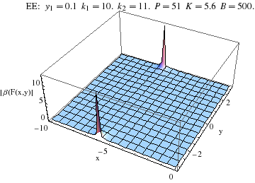
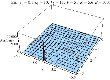
Figure 6: $|\beta(F(z))|$ as a function of $z\equiv\ln(Q^{2}/Q^{2}_{\rm in})=x+iy$, as in Fig. 3(a), but now with the modified beta function with $P=51$ ($=2N+1$), $K=5.6$ and $B=500$; the right-hand figure has more details around the pole. No Landau singularities (i.e., singularities inside the $z$ stripe) appear.

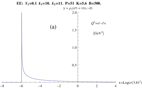
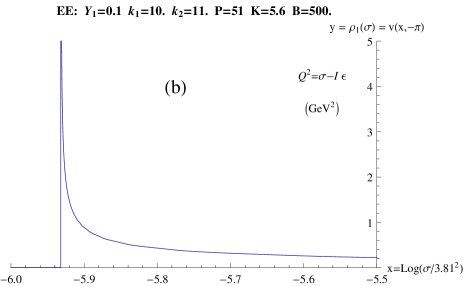
Figure 7: (a) The discontinuity function $\rho_{1}(\sigma)={\rm Im}\ a(Q^{2}=-\sigma-i\epsilon)={\rm Im}F(z=x-i\pi)=v(x,y=-\pi)$ as a function of $x={\rm Re}(z)=\ln(\sigma/Q^{2}_{\rm in})$, for the EE case with modified beta function ($P=51$, i.e., $N=25$); (b) enlarged picture around the threshold.

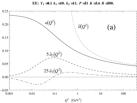
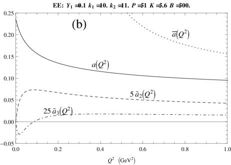
Figure 8: (a) The running coupling $a(Q^{2})$ as a function of positive $Q^{2}$, for the EE case with modified beta function ($P=51$, i.e., $N=25$), when $Q^{2}$ is on a logarithmic scale; included are the logarithmic derivatives ${\widetilde{a}}_{2}(Q^{2})$ and ${\widetilde{a}}_{3}(Q^{2})$, Eq. (51), rescaled by factors $5$ and $25$ for better visibility; for comparison, the corresponding $\overline{\rm MS}$ coupling ${\overline{a}}(Q^{2})$ is included; (b) same as in Fig. (a), but on linear $Q^{2}$ scale for low positive $Q^{2}$.

For this, we present in Figs. 6 the behavior of the function $|\beta(F(z))|$ for the EE case with $N=25$ (i.e., $P\equiv 2N+1=51$), which clearly indicates that there are no Landau singularities. In addition, in Figs. 7 we present for this case the discontinuity function $\rho_{1}(\sigma)\equiv{\rm Im}a(-\sigma-i\epsilon)$ as a function of $\ln(\sigma/Q^{2}_{\rm in})$, and in Figs. 8 the running coupling $a(Q^{2})$, and its logarithmic derivatives ${\widetilde{a}}_{2}(Q^{2})$ and ${\widetilde{a}}_{3}(Q^{2})$ [defined in Eq. (51)], for positive $Q^{2}$.

While the considered perturbative beta functions modified by the factor (21) give us simultaneously the correct value of $r_{\tau}$ and perturbative holomorphic coupling $a(Q^{2})$, one may worry that the introduction of the large coefficients $\sim B^{2N+1}$ (where $B\sim 10^{3}$) in the beta function [cf. Eq. (22)] represents an anomalous mass independent renormalization scheme, in the sense that the growth of the coefficients of beta function at large order becomes responsible for a growth of the coefficients of the physical spacelike physical quantities which is faster than the growth coming from the leading (UV or IR) renormalon. Here we will argue that if $P\equiv 2N+1$ in (21) is large enough, e.g. $P\geq 51$, then the renormalon growth of the coefficients will dominate over the growth from the beta function coefficients. For example, in the case of the timelike quantity $r_{\tau}$, the underlying spacelike quantity is Adler function $d(Q^{2})$ (with $N_{f}=3$), cf. Eq. (49).

Let us consider a general spacelike physical quantity ${\cal D}(Q^{2})$, whose expansion is

$${\cal D}(Q^{2})=a(Q^{2})+d_{1}a(Q^{2})^{2}+\cdots+d_{n}a(Q^{2})^{n+1}+\cdots$$ (24)

The expansion of its Borel transform is

$$B_{\cal D}(b)=1+\frac{d_{1}}{1!\beta_{0}}b+\cdots\frac{d_{n}}{n!\beta_{0}^{n}}b^{n}+\cdots\ .$$ (25)

It turns out that this function can have (renormalon) poles only at nonzero integer values $b=\pm 1,\pm 2,\ldots$, cf. Ref. Beneke:1998ui . The closer the renormalon pole is to the origin, the faster is the increase of the coefficients $d_{n}$ with $n$. Let us assume that the pole is at either $b=1$ or $b=-1$. Then, in the large-$\beta_{0}$ approximation, the coefficients $d_{n}$ behave at large $n$ as

$$|d_{n}|\approx{\cal K}n!\beta_{0}^{n}\sim n!\beta_{0}^{n}\ ,$$ (26)

where ${\cal K}\sim 1$. We recall that in our notation, $a\equiv\alpha_{s}/\pi$ and $\beta_{0}=(1/4)(11-2N_{f}/3)$, i.e., $\beta_{0}=9/4$ when $N_{f}=3$. On the other hand, the perturbative scheme independence of the physical quantity ${\cal D}(Q^{2})$ implies that the coefficient $d_{n}$ has a specific dependence on the scheme coefficients $c_{2},c_{3},\ldots,c_{n}$ of the beta function expansion (2). In particular, the dependence on $c_{n}$ is

$$d_{n}(c_{n},c_{n-1},\ldots,c_{2})=-\frac{1}{n-1}c_{n}+f_{n}(c_{n-1},\ldots,c_{2})\ .$$ (27)

On the other hand, it is straightforward to check that for the beta function (23) modified by the factor (21), with $B\sim 10^{3}$, $K\sim 10^{1}$ and $P=2N+1$, the first anomalous (large) beta coefficient is

$$c_{2P+2}\approx(-1)^{P+1}\frac{K}{a_{0}^{2}}\left(\frac{B}{a_{0}^{2}}\right)^{P}\ .$$ (28)

This implies, together with Eq. (27), that the first $d_{n}$ with anomalously large beta coefficient is

$$d_{2P+2}=\frac{(-1)^{P}}{2P+1}\frac{K}{a_{0}^{2}}\left(\frac{B}{a_{0}^{2}}\right)^{P}+\ldots\ ,$$ (29)

where the dots stand for a contribution that is independent of the anomalous scheme parameter $B$. We require that the contribution (29) of the anomalous scheme to the coefficient $d_{2P+2}$ is less than the contribution of the $b=\pm 1$ (leading) renormalon (26), and this implies

$$\frac{1}{2P+1}\frac{K}{a_{0}^{2}}\left(\frac{B}{a_{0}^{2}}\right)^{P} < (2P+2)!\beta_{0}^{2P+2}$$

$$\Rightarrow\;rat(P) \equiv \frac{KB^{p}}{a_{0}^{2P+2}(2P+1)(2P+2)!\beta_{0}^{2P+2}}<1$$ (30)

In the considered case of EE with $N=25$ ($P=51$), i.e., the last line of Table 2, it turns out that this ratio $rat(P)$ is $0.09$, i.e., the $b=\pm 1$ renormalon growth of the coefficients $d_{n}$ clearly dominates over the growth of $d_{n}$ coming from the scheme. For the other two cases (P[1/1] and P[1/0]) in Table 2, this ratio is still huge, primarily due to the larger value of $B$ ($\approx 2000$), and a significantly larger value of $P$ is needed. If the renormalon effects are accounted for beyond the large-$\beta_{0}$ approximation, the growth of the coefficients $d_{n}$ becomes even slightly faster Beneke:1998ui . Furthermore, in the specific case of $r_{\tau}$, where the underlying coefficients $d_{n}$ are those of Adler function, the leading renormalon is at $b=-1$ and it is double (quadratic), so that the $|d_{n}|$ coefficients grow even slightly faster than in Eq. (26), as $\sim(n+1)!\beta_{0}^{n}$.

V Borel sum rules in V+A channel of tau lepton semihadronic decays

In this Section we extract the four and six-dimensional condensates $\langle O_{4}^{\rm(V+A)}\rangle=(1/6)\langle aG^{\alpha}_{\mu\nu}G^{\alpha}_{\mu\nu}\rangle$ and $\langle O_{6}^{\rm(V+A)}\rangle$ appearing in the Operator product expansion (OPE) of the $V+A$ quark current correlator $\Pi(Q^{2})$, based on the measurements of the $\tau$-lepton semihadronic decays. We use the Borel transform sum rules, following closely the approach of Ref. anOPE , where the evaluation was performed for the (nonperturbative) $2$-delta analytic QCD (2$\delta$anQCD) model of Ref. 2danQCD . That approach followed the Borel transform sum rule methods of Refs. Geshkenbein ; Ioffe . We outline only the main features of the approach and refer for details of the approach to Ref. anOPE and Ref. Ioffe .

The starting point is the identity (sum rule)

$$\int_{0}^{\sigma_{0}}d\sigma g(-\sigma)\omega_{\rm exp}(\sigma)=-i\pi\oint_{|Q^{2}|=\sigma_{0}}dQ^{2}g(Q^{2})\Pi_{\rm th}(Q^{2})\ ,$$ (31)

where $g(Q^{2})$ is an analytic (holomorphic) function in the entire $Q^{2}$ complex plane, which characterizes the specific sum rule. The contour integration on the right-hand side is in the counterclockwise direction, and $\omega(\sigma)$ is the spectral function of the $V+A$ quark current correlator function $\Pi(Q^{2})$

$$\omega(\sigma)\equiv 2\pi\;{\rm Im}\ \Pi(Q^{2}=-\sigma-i\epsilon)\ .$$ (32)

The identity (31) comes from applying the Cauchy theorem to the function $g(Q^{2})\Pi(Q^{2})$ and accounting for the correct holomorphic behavior of the correlator $\Pi(Q^{2})$ as required by the general principles of quantum field theories. The same type of holomorphic behavior is respected by the QCD running couplings $a(Q^{2})$ and ${\widetilde{a}}_{n}(Q^{2})$ in the schemes considered in this work. Therefore, the theoretically evaluated correlators $\Pi_{\rm th}(Q^{2})$ [$\Leftrightarrow{\cal D}_{\rm Adl}(Q^{2})$], at each order of truncation in the considered holomorphic schemes, have the analytic behavior consistent with the identity (31).

In the present case, we are interested in $V+A$ channel of $\tau$ lepton semihadronic nonstrange decays. The experimental spectral function $\omega_{\rm exp}(\sigma)$ on the left-hand side of the sum rule (31) is obtained from the invariant-mass spectra of the $\tau$ lepton strangeless decays with the squared invariant mass $\sigma$ in the interval $0<\sigma<\sigma_{0}$. Our analysis here is based on the data of ALEPH Collaboration ALEPH1 ; ALEPH2a ; ALEPH2b . On the right-hand side of the sum rule is the correlator function $\Pi(Q^{2})$, which is theoretically evaluated with OPE

$$\Pi(Q^{2})=-\frac{1}{2\pi^{2}}\ln(Q^{2}/\mu^{2})+\Pi(Q^{2};D\!=\!0)+\sum_{n\geq 2}\frac{\langle O_{2n}\rangle}{(Q^{2})^{n}}\left(1+{\cal C}_{n}a(Q^{2})\right)\ .$$ (33)

Note that $n=D/2$ where $D$ denotes the operator dimension of the local operators contributing to the OPE of $\Pi(Q^{2})$. The $D=2$ ($n=1$) term is proportional to the current masses of $u$ and $d$ quarks, and is negligible. For us the relevant terms are $D=4,6$ ($n=2,3$). Further, it can be checked that the terms proportional to ${\cal C}_{n}a(Q^{2})$ will be negligible in the Borel sum rules applied here (cf. footnote 20 of Ref. anOPE ).

For the evaluation of the right-hand side of the sum rule (31), it turns out convenient to integrate it by parts

$$\int_{0}^{\sigma_{0}}d\sigma g(-\sigma)\omega_{\rm exp}(\sigma)=-\frac{i}{2\pi}\int_{\phi=-\pi}^{\pi}\frac{dQ^{2}}{Q^{2}}{\cal D}_{\rm Adl}(Q^{2})\left[{\cal G}(Q^{2})-{\cal G}(-\sigma_{0})\right]{\big{|}}_{Q^{2}=\sigma_{0}\exp(i\phi)}\ ,$$ (34)

where ${\cal G}$ is any function satisfying

$$\frac{d{\cal G}(Q^{2})}{dQ^{2}}=g(Q^{2})\ ,$$ (35)

and ${\cal D}_{\rm Adl}(Q^{2})$ is the full massless Adler function

$${\cal D}_{\rm Adl}(Q^{2}) \equiv -2\pi^{2}\frac{d\Pi(Q^{2})}{d\ln Q^{2}}$$ (36a)

$$= 1+d(Q^{2})+2\pi^{2}\sum_{n\geq 2}\frac{n\langle O_{2n}\rangle}{(Q^{2})^{n}}\ ,$$ (36b)

where the terms with ${\cal C}_{n}a(Q^{2})$ were neglected, as mentioned earlier. The dimension $D=0$ part of the correlator is directly related to the (strangeless and massless) canonical Adler function $d(Q^{2})$ of Appendix A [Eqs. (50), (56)-(59)]

$$d(Q^{2})=-2\pi^{2}\frac{d\Pi(Q^{2};D\!=\!0)}{d\ln Q^{2}}\ .$$ (37)

In the sum rule (31), the analytic function $g(Q^{2})$ is usually taken to be either an exponential function $\propto\exp(Q^{2}/M^{2})$ (Borel sum rules, Refs. Ioffe ; Ioffe:2000ns ), or a Gaussian function $\propto\exp((Q^{2}/M^{2})^{2})$ (Gaussian sum rules, Ref. Ioffe:2000ns ), or powers $\propto(Q^{2})^{N}$. The integrals of the latter approach are called moments, and the corresponding sum rules are usually called finite energy sum rules, cf. Refs. Ioffe:2000ns ; vsr1 ; vsr2 ; vsr3 ; vsr4 ; vsr5 ; vsr6 ; vsr7 ; vsr8 .

Although the approach with moments is more widely used in the literature, we will calculate the Borel transforms, i.e., we will apply the Borel sum rules Ioffe , the main reason being that we already have experience and acquired confidence in such calculations, cf. Ref. anOPE . Nonetheless, it would be interesting to apply in the future the moment approach to the considered holomorphic schemes.

Therefore, our choice for $g(Q^{2})$ here will be

$$g(Q^{2})=\frac{1}{M^{2}}\exp(Q^{2}/M^{2})\ ,\qquad{\cal G}(Q^{2})=\exp(Q^{2}/M^{2})\ ,$$ (38)

where $M^{2}$ are chosen complex scales with ${\rm Re}(M^{2})>0$. The expressions in the sum rules (31) and (34) become Borel transforms $B(M^{2})$, and we choose there for the upper integration bound the maximal possible value $\sigma_{0}=m_{\tau}^{2}$ ($\approx 3.16\ {\rm GeV}^{2}$). The Borel sum rule thus has the form

$$B_{\rm exp}(M^{2})=B_{\rm th}(M^{2})\ ,$$ (39)

where

$$B_{\rm exp}(M^{2}) \equiv \int_{0}^{m_{\tau}^{2}}\frac{d\sigma}{M^{2}}\;\exp(-\sigma/M^{2})\omega_{\rm exp}(\sigma)\ ,$$ (40a)

$$B_{\rm th}(M^{2}) \equiv B(M^{2};D\!=\!0)+2\pi^{2}\sum_{n\geq 2}\frac{\langle O_{2n}\rangle}{(n-1)!\;(M^{2})^{n}}\ ,$$ (40b)

The $D=0$ part is

$$B(M^{2};D\!=\!0)=\left(1-\exp(-m_{\tau}^{2}/M^{2})\right)$$ (41)

$$+\frac{1}{2\pi}\int_{-\pi}^{\pi}d\phi\;d(Q^{2}\!=\!m_{\tau}^{2}e^{i\phi})\left[\exp\left(\frac{m_{\tau}^{2}e^{i\phi}}{M^{2}}\right)-\exp\left(-\frac{m_{\tau}^{2}}{M^{2}}\right)\right].$$

For small positive ${\rm Re}(M^{2})$, the Borel transform suppresses strongly the contributions of $\omega_{\rm exp}(\sigma)$ at high energies (high $\sigma$) where the experimental errors are larger. Further, the OPE higher dimension terms are suppressed in the Borel transform by a factor $1/(n-1)!$. In the real part of the Borel transform, OPE term contributions of specific dimension $D$ are eliminated if the complex scales $M^{2}$ are chosen along specific rays $M^{2}=|M^{2}|\exp(i\psi)$ in the complex plane. This facilitates the determination of the remaining condensates $\langle O_{2n}\rangle$ by comparing the theoretical expressions with the experimental values ${\rm Re}{\rm B}_{\rm exp}(|M^{2}|\exp(i\psi))$. For example, if $\psi=\pi/6,\pi/4$, then $D=6,4$ terms do not contribute, respectively, because ${\rm Re}(\exp(i\pi/2))=0$. Therefore, when ignoring terms with $D>6$, we have

$${\rm Re}B_{\rm exp}(|M|^{2}e^{i\pi/6}) = {\rm Re}B(|M|^{2}e^{i\pi/6};D\!=\!0)+\pi^{2}\frac{\langle O_{4}\rangle}{|M|^{4}}\ ,$$ (42a)

$${\rm Re}B_{\rm exp}(|M|^{2}e^{i\pi/4}) = {\rm Re}B(|M|^{2}e^{i\pi/4};D\!=\!0)-\pi^{2}\frac{\langle O_{6}\rangle}{\sqrt{2}|M|^{6}}\ ,$$ (42b)

We note that in the considered $V+A$ channel, the $D=4$ operator is proportional to the gluon condensate

$$\langle O_{4}^{(V+A)}\rangle=\frac{1}{6}\langle aG^{\alpha}_{\mu\nu}G^{\alpha}_{\mu\nu}\rangle\ ,$$ (43)

and the $D=6$ operator, in the vacuum saturation approximation, is nonnegative and proportional to the square of the quark-antiquark condensate Geshkenbein ; Ioffe

$$\langle O_{6}^{(V+A)}\rangle\approx\frac{128\pi^{2}}{81}a\langle{\overline{q}}q\rangle^{2}\ .$$ (44)

Here, as throughout this work, the notation $a\equiv\alpha_{s}/\pi$ is used.

The experimental values ${\rm Re}B_{\rm exp}(|M^{2}|\exp(i\psi))$ we use here are those of Figs. 4 and 5(a),(b) of Ref. Geshkenbein (they were used also in Ref. anOPE ), which are based on the values $\omega_{\rm exp}(\sigma)$ of the ALEPH 1998 data ALEPH1 . For the theoretical values ${\rm Re}B_{\rm th}(|M^{2}|\exp(i\psi))$, the evaluation of the contour integrals (41) of the canonical Adler function $d(Q^{2})$ was performed with renormalization scale $\mu^{2}=Q^{2}$, in the EE renormalization scheme: beta function (23) with $f(Y)$ of Eq. (12) [with $Y_{1}=0.1$; $k_{1}=10.$; $k_{2}=11.$] and ${\cal F}_{\rm fact}$ of the form (21) with $B=500$, $K=5.6$ and $P\equiv 2N+1=51$. For completeness, we write down here also values of the other beta function parameters $Y_{2}$ and $a_{0}\equiv{\mathcal{A}}_{1}(0)$ in this specific EE scheme, obtained numerically through the conditions (9b)-(9c) applied to $f_{\rm new}(Y)\equiv f(Y){\cal F}_{\rm fact}(Y)$: $Y_{2}=0.1839408532$ and $a_{0}=0.2360296246$. We choose this scheme because, as shown hitherto in this work, it represents an analytic (holomorphic) perturbative QCD, gives the correct value of $r_{\tau}$ decay ratio (cf. the last line in Table 2) and the growth of the coefficients $d_{n}$ with rising $n$ is dominated by the leading renormalon $b=\pm 1$ (cf. the previous Section) and not by the beta function.

Furthermore, $r_{\tau}$ was calculated in the LB+bLB approach, which is applicable if the running coupling $a(Q^{2})$ is holomorphic and which uses the maximal amount of the presently available information on the perturbation coefficients of Adler function, and is thus considered as one of the most effective resummation approaches for the $\tau$ decay physics quantities. Therefore, we apply the LB+bLB approach also in the calculation of the contour integrals (41) for the Borel sum rules. We refer to Appendix C for some formal details of the LB+bLB approach to the Borel sum rules (analogous to Appendix A which explains the calculation of $r_{\tau}$ in LB+bLB approach).

The experimental and the theoretical results are given in Figs. 9(a),(b) for $\psi\equiv{\rm arg}(M^{2})=\pi/6$, $\pi/4$, respectively, for the interval $0.68\ {\rm GeV}^{2}<|M^{2}|<1.50\ {\rm GeV}^{2}$.

Figure 9: (a) ${\rm Re}B(M^{2})$ for $M^{2}=|M^{2}|\exp(i\pi/6)$; (b) for $M^{2}=|M^{2}|\exp(i\pi/4)$. The grey band represents the experimental data. In Fig. (a), the (EE scheme) theoretical curves correspond to $\langle aG^{\alpha}_{\mu\nu}G^{\alpha}_{\mu\nu}\rangle=(0.010\pm 0.005)\ {\rm GeV}^{4}$; the $\overline{\rm MS}$ curve with $\langle aG^{\alpha}_{\mu\nu}G^{\alpha}_{\mu\nu}\rangle=0.0059\ {\rm GeV}^{4}$ is included as the dotted curve. In Fig. (b), the (EE scheme) theoretical curves correspond to $\langle O^{\rm(V+A)}\rangle_{6}=(0\pm 0.001)\ {\rm GeV}^{6}$; the $\overline{\rm MS}$ curve with $\langle O^{\rm(V+A)}\rangle_{6}=-1.8\times 10^{-3}\ {\rm GeV}^{6}$ is included as the dotted curve.

Comparison of the (EE scheme) theoretical curves with the experimental bands allows us to make an “educated guess” estimate of the condensate values

$$\langle aG^{\alpha}_{\mu\nu}G^{\alpha}_{\mu\nu}\rangle = (0.010\pm 0.005)\ {\rm GeV}^{4}\ ,$$ (45a)

$$\langle O_{6}^{\rm(V+A)}\rangle = (0\pm 0.001)\ {\rm GeV}^{6}\ .$$ (45b)

This can be compared with the values extracted by the Borel sum rule approach in $\overline{\rm MS}$ scheme [where truncated series is taken for $d(Q^{2})$] in Ref. anOPE : $\langle aGG\rangle=(0.0059\pm 0.0049)\ {\rm GeV}^{4}$ and $\langle O_{6}^{\rm(V+A)}\rangle=(-1.8\pm 0.9)\times 10^{-3}\ {\rm GeV}^{6}$. It is interesting that at $\psi=\pi/4$ we extract (in the EE scheme) the values of $\langle O_{6}^{\rm(V+A)}\rangle$, Eq. (45b), which are compatible with nonnegative values. This nonnegativity is compatible with the expectation based on the vacuum saturation approximation Eq. (44). On the other hand, the extracted values of $\langle O_{6}^{\rm(V+A)}\rangle$ in the $\overline{\rm MS}$ Borel sum rule approach are not compatible with the nonnegativity Eq. (44).

Figure 10: $B(M^{2})$ for $M^{2}=|M^{2}|$ (positive) scales. The grey band represents the experimental data. In Fig. (a), the (EE scheme) theoretical curves correspond to $\langle aG^{\alpha}_{\mu\nu}G^{\alpha}_{\mu\nu}\rangle=(0.010\pm 0.005)\ {\rm GeV}^{4}$ and the central value $\langle O_{6}^{\rm(V+A)}\rangle=0$. In Fig. (b), the (EE scheme) theoretical curves correspond to $\langle O_{6}^{\rm(V+A)}\rangle=(0\pm 0.001)\ {\rm GeV}^{6}$ and the central value $\langle aG^{\alpha}_{\mu\nu}G^{\alpha}_{\mu\nu}\rangle=0.010\ {\rm GeV}^{4}$. For comparison, the $\overline{\rm MS}$ curve is included in both figures as the dotted line, with its own central values $\langle aG^{\alpha}_{\mu\nu}G^{\alpha}_{\mu\nu}\rangle=0.0059\ {\rm GeV}^{4}$ and $\langle O_{6}^{\rm(V+A)}\rangle=(-1.8)\times 10^{-3}\ {\rm GeV}^{6}$.

In Figs. 10(a),(b) we present the experimental and theoretical results for $\psi\equiv{\rm arg}(M^{2})=0$: in Fig. 10(a) for the choice of the obtained central value of $\langle O_{6}^{\rm(V+A)}\rangle$ [$=0$, Eq. (45b)], varying $\langle aG^{\alpha}_{\mu\nu}G^{\alpha}_{\mu\nu}\rangle$ in the obtained interval (45a); in Fig. 10(b) for the choice of the obtained central value of $\langle aG^{\alpha}_{\mu\nu}G^{\alpha}_{\mu\nu}\rangle$ [$=0.010\ {\rm GeV}^{4}$, Eq. (45a)], varying $\langle O_{6}^{\rm(V+A)}\rangle$ in the obtained interval (45b). Comparison with the experimental band for $\psi=0$ indicates a good agreement, especially for the theoretical central (full line) curve. Furthermore, comparison with the $\overline{\rm MS}$ $\psi=0$ curve (with its own central values $0.0059\ {\rm GeV}^{4}$ and $-1.8\times 10^{-3}\ {\rm GeV}^{6}$) indicates that the obtained central curve of the EE scheme is better.

In Table 3, we display various terms in the evaluation of the real part of the Borel transform $B(M^{2})$, in the EE scheme (analytic) pQCD, with the LB+bLB approach, for various values of the complex scale $M^{2}$: $M^{2}=0.8\exp(i\psi)\ {\rm GeV}^{2}$ and $M^{2}=1.2\exp(i\psi)\ {\rm GeV}^{2}$, with $\psi=\pi/6$, $\pi/4$, $0$. These terms are based on the OPE expansion (40b), where for $D=4$ and $D=6$ condensates we take our central extracted values. The $D=0$ contribution is given in Appendix C, Eq. (72), in conjunction with Eqs. (73b) and (81). We denote as “LO” term the real part of the first term in Eq. (72), i.e., ${\rm Re}(1-\exp(-m_{\tau}^{2}/M^{2}))$, which comes from the first (unity) term in the expansion of the full Adler function, Eq. (36b).

Table 3: Various contributions to the real part ${\rm Re}B(M^{2})$ of the Borel transform in the LB+bLB approach, in the (analytic) EE scheme pQCD, for various complex scales: $M^{2}=0.8\exp(i\psi)\ {\rm GeV}^{2}$ and $M^{2}=1.2\exp(i\psi)\ {\rm GeV}^{2}$, with $\psi=\pi/6$, $\pi/4$, $0$. The various contributions are those indicated in Eq. (40b) and Eq. (72), in conjunction with Eqs. (73b) and (81). The “LO” term is the leading term ${\rm Re}(1-\exp(-m_{\tau}^{2}/M^{2}))$ in Eq. (72). For the $D=4$ term we used the central extracted value $\langle O_{4}^{\rm(V+A)}\rangle\equiv(1/6)\langle aGG\rangle=(1/6)\times 0.010\ {\rm GeV}^{2}$; the $D=6$ term is taken to be zero, in accordance with the central extracted value $\langle O_{6}^{\rm(V+A)}\rangle=0$.

$|M^{2}|$	${\rm arg}(M^{2})$	${\rm Re}B$: LO	${\rm Re}B$: LB	NLB	${\rm N}^{2}{\rm LB}$	${\rm N}^{3}{\rm LB}$	sum ${\rm Re}B(D=0)$	${\rm Re}B(D=4)$	${\rm Re}B$
0.8	$\pi/6$	1.01284	0.134652	0.000843	0.080223	0.009826	1.23839	0.025702	1.26409
1.2	$\pi/6$	0.974163	0.120230	0.000719	0.067647	0.008934	1.17169	0.011423	1.18311
0.8	$\pi/4$	1.05762	0.137521	0.000843	0.081522	0.011219	1.28873	0	1.28873
1.2	$\pi/4$	1.04447	0.124725	0.000727	0.068476	0.009661	1.24806	0	1.24806
0.8	0	0.980691	0.132679	0.0008434	0.079016	0.008587	1.20182	0.051404	1.25322
1.2	0	0.928025	0.117452	0.000715	0.067111	0.008301	1.1216	0.022846	1.14445

From the Table we can see that the LB+bLB series has a rather good convergence behavior. Namely, the LB term is always significantly larger than the bLB contribution.

While the theoretical curves and experimental bands shown in Figs. 9 can be interpreted as representing an extraction of the $D=4$ and $D=6$ condensate values Eqs. (45), the resulting theoretical curves in Figs. 10 represent our theoretical predictions for the Borel transform $B(M^{2})$ for a continuous set of (positive) scales $M^{2}$ as compared to the corresponding experimental values.

The extracted values (45) can be compared with the corresponding values obtained in the literature. The spread of these extracted values is usually $\delta\langle aGG\rangle\approx\pm 0.005\ {\rm GeV}^{4}$ and $\delta\langle O_{6}^{\rm(V+A)}\rangle\approx\pm 10^{-3}\ {\rm GeV}^{6}$, if the experimental uncertainties (the spread of the grey bands) are considered to be the dominant source of the uncertainties.

In Ref. anOPE , where the Borel transform sum rules were used, the extracted values for the gluon condensate were $\langle aGG\rangle\approx(0.006\pm 0.005)\ {\rm GeV}^{4}$ for the $\overline{\rm MS}$ (truncated) and the resummed Lambert scheme pQCD and 2$\delta$anQCD model; $(0.010\pm 0.006)\ {\rm GeV}^{4}$ for the 2$\delta$anQCD model (truncated); $(0.012\pm 0.005)\ {\rm GeV}^{4}$ for the Lambert scheme pQCD (truncated). Here, the Lambert scheme was the scheme used for the 2$\delta$anQCD analytic model of Ref. 2danQCD ($c_{2}\equiv\beta_{2}/\beta_{0}=-4.76$; $c_{3}=c_{2}^{2}/c_{1}\approx 12.74$; etc.). The truncated results were those based on the truncated series of the canonical Adler function $d(Q^{2})$ (including $\sim a^{4}$); the resummed versions were those based on a $[2/2]$-Padé-related resummation of that truncated series (cf. Ref. anOPE for more details). Further, the approximate values of the $D=6$ condensate $\langle O_{6}^{\rm(V+A)}\rangle$ extracted in Ref. anOPE were approximately $(-2\pm 1)\times 10^{-3}\ {\rm GeV}^{6}$ for the aforementioned approaches ($\overline{\rm MS}$ truncated; Lambert scheme pQCD truncated and resummed; 2$\delta$anQCD truncated), with the exception of the resummed 2$\delta$anQCD where it was $(-0.5\pm 1.1)\times 10^{-3}\ {\rm GeV}^{6}$.

On the other hand, earlier analyses with Borel transform sum rules, performed in $\overline{\rm MS}$ scheme, gave Geshkenbein $\langle aGG\rangle=(0.006\pm 0.012)\ {\rm GeV}^{4}$ and Ioffe $(0.005\pm 0.004)\ {\rm GeV}^{4}$. In Ref. O6sr1 , weighted finite energy sum rules and ALEPH 2005 data were used; the obtained values were $\langle aGG\rangle=(0.008\pm 0.005)\ {\rm GeV}^{4}$. In the original work on sum rules, Ref. Shifman1 ; Shifman2 , the value $\langle aGG\rangle=0.012\ {\rm GeV}^{4}$ was obtained, using charmonium physics. Application of the QCD-moment and QCD-exponential moment sum rules for heavy quarkonia, Refs. O4sr1a ; O4sr1b , gave there the values $\langle aGG\rangle=(0.022\pm 0.004)\ {\rm GeV}^{4}$ and $(0.024\pm 0.006)\ {\rm GeV}^{4}$, respectively. Furthermore, a combined fit of the $V+A$ channel $\tau$ decay data, Ref. DDHMZ , extracted the value of $\alpha_{s}$ and, as a byproduct, the condensate value $\langle aGG\rangle=(-0.015\pm 0.003)\ {\rm GeV}^{4}$.

Most of the analyses in the literature give $\langle O_{6}^{\rm(V+A)}\rangle<0$, cf. Refs. O6sr1 ; O6sr2 ; anOPE , suggesting a qualitative failure of the vacuum saturation approximation Eq. (44), in contrast to the result (45b) obtained here in the considered analytic pQCD in the EE scheme.

VI Conclusions

We constructed a perturbative mass independent beta function $\beta(a)$ for the QCD running coupling $a(Q^{2})$ ($\equiv\alpha_{s}(Q^{2})/\pi$) at $N_{f}=3$ such that the following two restrictions are fulfilled simultaneously: (a) the correct value of the semihadronic strangeless tau lepton decay ratio $r_{\tau}\approx 0.203$ is reproduced, $r_{\tau}$ being here presently the best measured inclusive low-energy QCD quantity with strongly suppressed higher-twist contributions; (b) the coupling $a(Q^{2})$ has no (unphysical) Landau singularities, i.e., it is a holomorphic function in the complex $Q^{2}$ plane $Q^{2}\in\mathbb{C}\backslash(-\infty,-M_{\rm thr}^{2}]$, with a threshold mass $M_{\rm thr}\sim 0.1$ GeV. This construction was not straightforward, because the two mentioned conditions tend to mutually exclude each other. In contrast to the results of Refs. anpQCD1 ; anpQCD2 , where the growth of the coefficients $d_{n}$ of the spacelike physical quantities ${\cal D}(Q^{2})$ due to the scheme (beta function) was out of control already at $n=4$, we construct here beta functions which do not lead to an explosive growth of the coefficients $d_{n}$, at least up to a given chosen order $n$. In one case (EE scheme), we even obtained a beta function which contributes for large $n$ to the growth of the coefficients $d_{n}$ less than the leading $b=\pm 1$ renormalon contributes. Stated otherwise, the effects of our perturbative beta function did not overshadow the renormalon growth of the coefficients $d_{n}$ and, at the same time, they eliminated the Landau singularities of the running coupling and allowed the reproduction of the correct value of $r_{\tau}$. The attractiveness of the obtained holomorphic (analytic) QCD models is that they are perturbative, i.e., beta function $\beta(a)$ is fully described by the Taylor series in powers of $a$, it has no nonperturbative contributions such as $\exp(-{\cal K}/a(Q^{2}))\sim 1/(Q^{2})^{M}$, in contrast to the presently known analytic QCD models Refs. ShS1 ; ShS2 ; MS ; Nest1a ; Nest1b ; Nest1c ; Nest1d ; Nest2a ; Nest2b ; Nest2c ; Webber ; CV12a ; CV12b ; Alekseev ; 1danQCD ; 2danQCD ; Shirkovmass ; mes2a ; mes2b ; Simonov1 ; Simonov2 ; BKSKKSh1 ; BKSKKSh2 ; BKSKKSh3 ; BKSKKSh4 ; BKSKKSh5 . In addition, with the EE scheme (analytic) pQCD, we performed an analysis with Borel sum rules for the $V+A$ channel of semihadronic strangeless decays of $\tau$ lepton, and extracted reasonable values of the corresponding condensates: $\langle aGG\rangle=(0.010\pm 0.005)\ {\rm GeV}^{4}$ and $\langle O_{6}^{\rm(V+A)}\rangle=(0\pm 0.001)\ {\rm GeV}^{6}$. It remains to be seen how the presented holomorphic pQCD models work in the evaluation of other low-momentum inclusive observables, such as Bjorken polarized sum rule (BSR). In contrast to the well-measured low-momentum quantity $r_{\tau}$ ($V+A$ channel), the BSR has strong chirality-conserving higher-twist effects at low momenta, which makes the evaluation of this quantity even in analytic QCD models more difficult Khandr1 ; Khandr2 ; Khandr3 ; Khandr4 .

Appendix A Leading-$\beta_{0}$ resummation of $r_{\tau}$ and beyond

In this Appendix, we summarize those parts of Appendices of Refs. anpQCD1 ; anpQCD2 that are relevant in this work.

The decay ratio of the semihadronic strangeless $\tau$ lepton decays (V+A)-channel is

$$R_{\tau}(\triangle S\!=\!0) \equiv \frac{\Gamma(\tau^{-}\to\nu_{\tau}{\rm hadrons}(\gamma))}{\Gamma(\tau^{-}\to\nu_{\tau}e^{-}{\overline{\nu}_{e}}(\gamma))}-R_{\tau}(\triangle S\!\not=\!0)$$ (46a)

$$= 3.479\pm 0.011\ ,$$ (46b)

where the measured value given above is extracted from measurements by the ALEPH Collaboration ALEPH2a ; ALEPH2b and updated in Ref. DDHMZ . The QCD canonic massless quantity $r_{\tau}(\triangle S=0,m_{q}=0)$ is obtained from this quantity by removing the non-QCD (CKM and EW) factors and contributions, and the chirality-violating quark mass contributions

$$r_{\tau}(\triangle S=0,m_{q}=0)=\frac{R_{\tau}(\triangle S=0)}{3|V_{ud}|^{2}(1+{\delta}_{{\rm EW}})}$$ (47)

$$-(1+\delta_{\rm EW}^{\prime})-\delta r_{\tau}(\triangle S=0,m_{u,d}\not=0)\ .$$

This quantity $r_{\tau}$ is QCD-canonic in the sense that its (leading-twist) pQCD expansion is $r_{\tau}(\triangle S=0,m_{q}=0)_{\rm pt}=a+{\cal O}(a^{2})$. The higher-twist massless contributions in this $r_{\tau}(V+A)$ are very suppressed DDHMZ . Further, it is a timelike quantity, and can be expressed in terms of the massless current-current correlation function (V-V or A-A, both equal since massless) Tsai:1971vv

$$r_{\tau}=\frac{2}{\pi}\int_{0}^{m^{2}_{\tau}}\ \frac{ds}{m^{2}_{\tau}}\left(1-\frac{s}{m^{2}_{\tau}}\right)^{2}\left(1+2\frac{s}{m^{2}_{\tau}}\right){\rm Im}\Pi(Q^{2}=-s)\ .$$ (48)

Using the Cauchy theorem in the complex $Q^{2}$ plane and integrating by parts results in the following contour integral form Bra1 ; Bra2 ; Bra3 ; Bra4 ; Pivovarov:1991rh ; LeDiberder:1992te ; Beneke:2008ad :

$$r_{\tau}=\frac{1}{2\pi}\int_{-\pi}^{+\pi}d\phi\ (1+e^{i\phi})^{3}(1-e^{i\phi})\ d(Q^{2}=m_{\tau}^{2}e^{i\phi})\ ,$$ (49)

where $d(Q^{2})=-d\Pi(Q^{2})/d\ln Q^{2}=a(Q^{2})+{\cal O}(a^{2})$ is the canonical massless Adler function, which is a spacelike QCD quantity whose expansion in powers $a^{n}$ and in logarithmic derivatives ${\widetilde{a}}_{n}$ is

$$d(Q^{2})_{\rm pt} = a(Q^{2})+\sum_{n=1}^{\infty}d_{n}a(Q^{2})^{n+1}\ ,$$ (50a)

$$d(Q^{2})_{\rm mpt} = a(Q^{2})+\sum_{n=1}^{\infty}{{\widetilde{d}}}_{n}{\widetilde{a}}_{n+1}(Q^{2})\ .$$ (50b)

Here, the logarithmic derivatives are defined as

$${\widetilde{a}}_{n+1}(\mu^{2})\equiv\frac{(-1)^{n}}{\beta_{0}^{n}n!}\left(\frac{\partial}{\partial\ln\mu^{2}}\right)^{n}a(\mu^{2})\ ,\qquad(n=1,2,\ldots)$$ (51)

and are related with the powers by (repeated) application of RGE

$${\widetilde{a}}_{2} = a^{2}+c_{1}a^{3}+c_{2}a^{4}+\cdots\ ,$$ (52a)

$${\widetilde{a}}_{3} = a^{3}+\frac{5}{2}c_{1}a^{4}+\cdots\ ,\qquad{\widetilde{a}}_{4}=a^{4}+\cdots\ ,\qquad{\rm etc.}$$ (52b)

These relations can be recursively inverted

$$a^{2} = {\widetilde{a}}_{2}-c_{1}{\widetilde{a}}_{3}+\left(\frac{5}{2}c_{1}^{2}-c_{2}\right){\widetilde{a}}_{4}+\cdots\ ,$$ (53a)

$$a^{3} = {\widetilde{a}}_{3}-\frac{5}{2}c_{1}{\widetilde{a}}_{4}+\cdots\ ,\qquad a^{4}={\widetilde{a}}_{4}+\cdots\ ,\qquad{\rm etc.}$$ (53b)

Inserting the relations (53) into the power series (50a), we immediately obtain the coefficients ${\widetilde{d}}_{n}$ of the “modified” perturbation series (50b) in logarithmic derivatives

$${\widetilde{d}}_{1} = d_{1}\ ,\qquad{\widetilde{d}}_{2}=d_{2}-c_{1}d_{1}\ ,$$ (54a)

$${\widetilde{d}}_{3} = d_{3}-\frac{5}{2}c_{1}d_{2}+\left(\frac{5}{2}c_{1}^{2}-c_{2}\right)d_{1}\ ,\qquad{\rm etc.}$$ (54b)

If the power series (50a) is used in the contour integral (49) and integrated for each term separately, then the obtained result is called the contour improved perturbation theory (CIPT) Pivovarov:1991rh ; LeDiberder:1992te . However, since we consider here such schemes in which $a(Q^{2})$ is holomorphic, there is another, probably better, approach available for the evaluation of the contour integral (49), which involves the so called leading-$\beta_{0}$ (LB) resummation and the subsequent addition of three other known terms. Namely, the coefficients ${\widetilde{d}}_{n}$ (and $d_{n}$) can be written as a power series of $N_{f}$, and thus as a power series of $\beta_{0}$ (because $N_{f}=-6\beta_{0}+33/2$)

$${\widetilde{d}}_{n}=c_{n,n}\beta_{0}^{n}+c_{n,n-1}\beta_{0}^{n-1}+\ldots+c_{n,0}\ ,$$ (55)

where ${\widetilde{d}}_{n}(LB)=c_{n,n}\beta_{0}^{n}$ is the LB part of the coefficient ${\widetilde{d}}_{n}$, it is scheme independent, and is known for every $n$, Refs. Broad1 ; Broad2 . It turns out that in the series (50b), the LB parts can be resummed Neubert ; logder1 ; logder2

$$d^{\rm(LB)}(Q^{2}) = a(\kappa Q^{2})+\sum_{n=1}^{\infty}c_{n,n}(\kappa)\;\beta_{0}^{n}\;{{\widetilde{a}}}_{n+1}(\kappa Q^{2})$$ (56a)

$$= \int_{0}^{\infty}\frac{dt}{t}\;F_{d}(t)\;a(tQ^{2}e^{{\overline{\cal C}}})\ ,$$ (56b)

where ${\overline{\cal C}}=-5/3$ in $\overline{\rm MS}$ scaling convention, and the characteristic function $F_{d}(t)$ for Adler function is known explicitly Neubert

$$F_{d}(t)_{(t<1)} = 2C_{F}t{\Big{[}}-t\ln(t)+(1+t)\ln(1+t)\ln(t)+\frac{7}{4}t$$ (57a)

$$+(1+t){\rm Li}_{2}(-t){\Big{]}}\ ,$$

$$F_{d}(t)_{(t>1)} = 2C_{F}{\Big{[}}\left(\frac{1}{2}+t\right)\ln(t)-t(1+t)\ln(t)\ln(1+1/t)+\left(\frac{3}{4}+t\right)$$ (57b)

$$+t(1+t){\rm Li}_{2}\left(-1/t\right){\Big{]}}\ .$$

In the expressions above, $C_{F}=(N_{c}^{2}-1)/(2N_{c})=4/3$. If $a(Q^{2})$ [and thus ${{\widetilde{a}}}_{n+1}(\kappa Q^{2})$] have Landau singularities at $0<Q^{2}\lesssim\ 1{\rm GeV}^{2}$, the resummation (56b) does not cure the problem of these singularities. In fact, it makes the problem formally even worse, as the integral (56b) is then undefined (ambiguous) for any $Q^{2}>0$, due to singularities in the integrand factor $a(tQ^{2}e^{{\overline{\cal C}}})$ at low $t$. On the other hand, if $a(Q^{2})$ is holomorhic, no (Landau) singularities are encountered and the LB-integral (56b) is convergent and unambiguous.

The entire canonical Adler function

$$d(Q^{2})=d^{\rm(LB)}(Q^{2})+d^{\rm(bLB)}(Q^{2})$$ (58)

consists of the LB-part (56), and of the beyond-the-leading-$\beta_{0}$ (bLB) contribution whose expansion is

$$d^{\rm(bLB)}(Q^{2}) = \sum_{n=1}^{\infty}T_{n}{{\widetilde{a}}}_{n+1}(Q^{2})=\sum_{n=1}^{\infty}({{\widetilde{d}}}_{n}-c_{n,n}\beta_{0}^{n}){{\widetilde{a}}}_{n+1}(Q^{2})\ .$$ (59)

Insertion of the LB-integral (56b) of Adler function into the contour integral (49) then gives us the LB-part of $r_{\tau}$

$$r_{\tau}^{\rm(LB)}=\int_{0}^{\infty}\frac{dt}{t}\>F_{r}^{\cal{M}}(t)\>{\mathfrak{A}}_{1}(te^{\cal C}m_{\tau}^{2})\ ,$$ (60)

where the superscript ${\cal{M}}$ indicates that these are Minkowskian (timelike) quantities; ${\mathfrak{A}}_{1}$ is the timelike coupling

$${\mathfrak{A}}_{1}(s) = \frac{1}{\pi}\int_{s}^{\infty}\frac{d\sigma}{\sigma}{\rho}_{1}(\sigma)\ ;$$ (61)

and the characteristic function $F_{r}^{\cal{M}}(t)$ was obtained in Ref. Neubert2 . Since $-\pi d{\mathfrak{A}}_{1}(s)/d\ln s=\rho_{1}(s)$, integration by parts allows us to express $r_{\tau}^{\rm(LB)}$ as an integral over the discontinuity function $\rho_{1}(s)\equiv{\rm Im}\;a(-s-i\epsilon)$

$$r_{\tau}^{\rm(LB)}=\frac{1}{\pi}\int_{0}^{\infty}\frac{dt}{t}\>{\widetilde{F}}_{r}(t)\>\rho_{1}(te^{\cal{\overline{C}}}m_{\tau}^{2})\ .$$ (62)

This form is convenient here since the numerical integration of the RGE (5) gives us the values of $\rho_{1}(s)$ [and not ${\mathfrak{A}}_{1}(s)$], cf. Figs. 5 and 7. The characteristic function

$${\widetilde{F}}_{r}(t)=\int_{0}^{t}\frac{dt^{\prime}}{t^{\prime}}\>F_{r}^{\cal{M}}(t^{\prime})$$ (63)

was obtained explicitly in Appendix of Ref. anpQCD1 (Appendix D of Ref. anpQCD2 ); here we only reproduce it in Figs. 11, for better visualization.

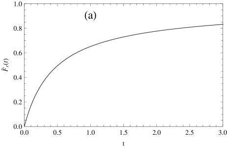
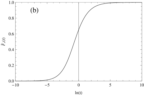
Figure 11: The function ${\widetilde{F}}_{r}(t)$ appearing in the integral (62) of $r_{\tau}^{\rm(LB)}$: (a) as function of $t$; (b) as function of $\ln t$.

However, the first three full (i.e., LB+beyond LB) coefficients $d_{1}$, $d_{2}$ and $d_{3}$ ($\Rightarrow$ ${\widetilde{d}}_{1}$, ${\widetilde{d}}_{2}$, ${\widetilde{d}}_{3}$) of the Adler function are known exactly d1a ; d1b ; d1c ; d2a ; d2b ; d3 . This means that we can add to the LB part (60) the beyond-the-leading-$\beta_{0}$ contributions (bLB) of order $\sim{\widetilde{a}}_{n}$ ($n=1,2,3$)

$$(r_{\tau})^{\rm(LB+bLB)}=r_{\tau}^{\rm(LB)}+\sum_{n=1}^{3}\ T_{n}I({\widetilde{a}}_{n+1})\ ,$$ (64)

where

$$T_{n} = {\widetilde{d}}_{n}-{\widetilde{d}}_{n}^{\rm(LB)}={\widetilde{d}}_{n}-c_{n,n}\beta_{0}^{n}\ ,$$ (65a)

$$I({\widetilde{a}}_{n+1}) = \frac{1}{2\pi}\int_{-\pi}^{+\pi}d\phi\ (1+e^{i\phi})^{3}(1-e^{i\phi})\ {\widetilde{a}}_{n+1}(m_{\tau}^{2}e^{i\phi})\ ,$$ (65b)

and $r_{\tau}^{\rm(LB)}$ is given in Eq. (62). We recall that in Eq. (65a) the part ${\widetilde{d}}_{n}^{\rm(LB)}=c_{n,n}\beta_{0}^{n}$ is scheme independent (i.e., independent of $c_{2},c_{3},\ldots$), and therefore $T_{n}$ has the same scheme dependence as ${\widetilde{d}}_{n}$. We consider the expression (64) in conjunction with Eq. (62) as the preferred method of evaluation, and we use it for our evaluations of $r_{\tau}$. Implicitly, we assume that the renormalization scale in $d(Q^{2}=m_{\tau}^{2}e^{i\phi})$ in the contour integral (49) is $\mu^{2}=Q^{2}$ [$=m_{\tau}^{2}e^{i\phi})$]; though, other renormalization scales could be used, e.g. $\mu^{2}=\kappa Q^{2}$ with $\kappa\not=1$ ($\kappa\sim 1$). Furthermore, we could use for the bLB contributions in Eq. (64) the powers $a^{n}$, i.e., the power series of $d(Q^{2})^{\rm(bLB)}\equiv d(Q^{2})-d(Q^{2})^{\rm(LB)}$ instead of the series in logarithmic derivatives; we do not prefer this choice, because the LB part $d(Q^{2})^{\rm(LB)}$ represents a (LB-)series (56a) in logarithmic derivatives ${\widetilde{a}}_{n}$ and not in powers $a^{n}$.

Appendix B Coefficients of perturbation expansion in a general scheme

In this Appendix we summarize the relations between the $\overline{\rm MS}$ scheme and general scheme coefficients in perturbation expansions of physical quantities. Perturbation expansions of spacelike observables ${\cal F}(Q^{2})$ are usually given in the literature in the $\overline{\rm MS}$ scheme

$${\cal F}(Q^{2})_{{\rm pt}\overline{\rm MS}} = {\overline{a}}^{\nu_{0}}+{\overline{\cal F}}_{1}{\overline{a}}^{1+\nu_{0}}+{\overline{\cal F}}_{2}{\overline{a}}^{2+\nu_{0}}+{\overline{\cal F}}_{3}{\overline{a}}^{3+\nu_{0}}+\ldots\ ,$$ (66)

where ${\overline{a}}$ is the coupling $a\equiv\alpha_{s}/\pi$ in the $\overline{\rm MS}$ renormalization scheme (${\overline{c}}_{2},{\overline{c}}_{3},\ldots$) and at the canonical renormalization scale $\mu^{2}=Q^{2}$

$${\overline{a}}\equiv a(\mu^{2}=Q^{2};{\overline{c}}_{2},{\overline{c}}_{3},\ldots)\ .$$ (67)

The coupling in a different renormalization scheme ($c_{2},c_{3},\ldots$) and at a general (spacelike) renormalization scale $\mu^{2}=\kappa Q^{2}$ (where $\kappa>0$, usually $\kappa\sim 1$)

$$a\equiv a(\mu^{2}=\kappa Q^{2};c_{2},c_{3},\ldots)$$ (68)

can be related to ${\overline{a}}$ by use of the relations (3) and (1)-(2) (cf. Appendix A of Ref. Stevenson , and Appendix A of Ref. CK )

$${\overline{a}} = a+a^{2}\beta_{0}\ln\kappa+a^{3}\left[\beta_{0}^{2}\ln^{2}\kappa+c_{1}\beta_{0}\ln\kappa-(c_{2}-{\overline{c}}_{2})\right]$$ (69)

$$+a^{4}\left[\beta_{0}^{3}\ln^{3}\kappa+\frac{5}{2}c_{1}\beta_{0}^{2}\ln^{2}\kappa+c_{2}\beta_{0}\ln\kappa-3(c_{2}-{\overline{c}}_{2})\beta_{0}\ln\kappa-\frac{1}{2}(c_{3}-{\overline{c}}_{3})\right]$$

$$+{\cal O}(a^{5})\ ,$$

where the notations used are those of Eq. (2), with $\beta_{0}=(1/4)(11-2N_{f}/3)$ and $c_{k}\equiv\beta_{k}/\beta_{0}$. Substituting the expansion (69) into the expansion (66), and performing power expansion there in powers of $a$, we obtain the perturbation expansion of the physical spacelike quantity ${\cal F}(Q^{2})$ expressed in the general scheme

$${\cal F}(Q^{2})_{\rm pt} = a^{\nu_{0}}+{\cal F}_{1}a^{1+\nu_{0}}+{\cal F}_{2}a^{2+\nu_{0}}+{\cal F}_{3}a^{3+\nu_{0}}+\ldots\ ,$$ (70)

where the new coefficients ${\cal F}_{j}$ are expressed by the original $\overline{\rm MS}$ “canonical” coefficients ${\overline{\cal F}}_{k}$ in the following way:

$${\cal F}_{1} = {\overline{\cal F}}_{1}+\nu_{0}\beta_{0}\ln\kappa,$$ (71a)

$${\cal F}_{2} = {\overline{\cal F}}_{2}+{\overline{\cal F}}_{1}(\nu_{0}+1)\beta_{0}\ln\kappa$$ (71b)

$$+\nu_{0}\left[\frac{1}{2}(\nu_{0}+1)\beta_{0}^{2}\ln^{2}\kappa+c_{1}\beta_{0}\ln\kappa-(c_{2}-{\overline{c}}_{2})\right],$$

$${\cal F}_{3} = {\overline{\cal F}}_{3}+{\overline{\cal F}}_{2}(\nu_{0}+2)\beta_{0}\ln\kappa$$ (71c)

$$+{\overline{\cal F}}_{1}(\nu_{0}+1)\left[\left(\frac{\nu_{0}}{2}+1\right)\beta_{0}^{2}\ln^{2}\kappa+c_{1}\beta_{0}\ln\kappa-(c_{2}-{\overline{c}}_{2})\right]$$

$$+\nu_{0}{\Big{[}}\frac{1}{6}(2+3\nu_{0}+\nu_{0}^{2})\beta_{0}^{3}\ln^{3}\kappa+\frac{1}{2}c_{1}(3+2\nu_{0})\beta_{0}^{2}\ln^{2}\kappa$$

$$+\left(c_{2}-(\nu_{0}+2)(c_{2}-{\overline{c}}_{2})\right)\beta_{0}\ln\kappa-\frac{1}{2}(c_{3}-{\overline{c}}_{3}){\Big{]}}.$$

Usually we have $\nu_{0}=1$, e.g., in the case of the Adler function $d(Q^{2})$ which is the underlying spacelike quantity for the (timelike) quantity $r_{\tau}$, cf. Eqs. (49)-(50). In general, the index $\nu_{0}$ may be noninteger, such as, for example, in the case of the underlying spacelike quantity for the (timelike) decay width of Higgs $\Gamma(H\to b{\bar{b}})$ BMS2 ; BMS3 ; GCAK .

Appendix C Leading-$\beta_{0}$ resummation in Borel sum rules and beyond

Here we present the calculation of the $D=0$ part of the (theoretical) Borel transform $B(M^{2})$ of Eq. (41), using the LB+bLB approach described in Appendix A. Applying the contour integration (41) with the canonical Adler function $d(Q^{2})$ written in the form (58), we obtain

$$B(M^{2};D=0)=\left(1-\exp(-m_{\tau}^{2}/M^{2})\right)+B^{\rm(LB)}(M^{2})+B^{\rm(bLB)}(M^{2})\ ,$$ (72)

where the bLB part is

$$B^{\rm(bLB)}(M^{2})=$$ (73a)

$$=\frac{1}{2\pi}\int_{-\pi}^{\pi}d\phi\;d^{\rm(bLB)}(Q^{2}\!=\!m_{\tau}^{2}e^{i\phi})\left[\exp\left(\frac{m_{\tau}^{2}e^{i\phi}}{M^{2}}\right)-\exp\left(-\frac{m_{\tau}^{2}}{M^{2}}\right)\right]$$

$$= \sum_{n=1}^{3}T_{n}\frac{1}{2\pi}\int_{-\pi}^{\pi}{\widetilde{a}}_{n+1}(Q^{2}\!=\!m_{\tau}^{2}e^{i\phi})\left[\exp\left(\frac{m_{\tau}^{2}e^{i\phi}}{M^{2}}\right)-\exp\left(-\frac{m_{\tau}^{2}}{M^{2}}\right)\right],$$ (73b)

where $T_{n}$ are the bLB coefficients appearing in Eqs. (59) and (65a). The summation over $n$ in Eq. (73b) was truncated at $n=3$, because only the first three coefficients $d_{1},d_{2},d_{3}$ ($\Rightarrow{\widetilde{d}}_{1},{\widetilde{d}}_{2},{\widetilde{d}}_{3}$) are known exactly d1a ; d1b ; d1c ; d2a ; d2b ; d3 .

The LB part in Eq. (72) is obtained in the following way. According to Eq. (40a) we have

$$B^{\rm(LB)}(M^{2})=\int_{0}^{m_{\tau}^{2}}\;\frac{d\sigma}{M^{2}}e^{-\sigma/M^{2}}\omega^{\rm(LB)}(\sigma)\ .$$ (74)

According to Eq. (32), we have

$$\omega^{\rm(LB)}(\sigma)=2\pi{\rm Im}\Pi^{\rm(LB)}(Q^{2}=-\sigma-i\epsilon)$$ (75a)

$$=i\pi\left[\Pi^{\rm(LB)}(Q^{2}=-\sigma+i\epsilon)-\Pi^{\rm(LB)}(Q^{2}=-\sigma-i\epsilon)\right]$$

$$= i\pi\int_{Q^{{}^{\prime}2}=-\sigma-i\epsilon}^{-\sigma+i\epsilon}d(\ln Q^{{}^{\prime}2})\frac{\partial\Pi^{\rm(LB)}(Q^{{}^{\prime}2})}{\partial\ln Q^{{}^{\prime}2}}=\frac{1}{2\pi i}\oint_{-\sigma-i\epsilon}^{-\sigma+i\epsilon}\frac{dQ^{{}^{\prime}2}}{dQ^{{}^{\prime}2}}d^{\rm(LB)}(Q^{{}^{\prime}2}).$$ (75b)

The contour integration in the two integrals in the complex $Q^{{}^{\prime}2}$ plane is counterclockwise along a circle of radius $\sigma$. We use in the last integral for the integrand $d^{\rm(LB)}(Q^{{}^{\prime}2})$ the integral expression (56b), and interchange the order of integration over $Q^{{}^{\prime}2}$ and $t$. This gives

$$\omega^{\rm(LB)}(\sigma)=\int_{0}^{\infty}\;\frac{dt}{t}F_{d}(t){\mathfrak{A}}_{1}(t\sigma e^{{\overline{\cal C}}})\ ,$$ (76)

where $F_{d}(t)$ is the characteristic function of the (LB) Adler function, given in Eqs. (57), and

$${\mathfrak{A}}_{1}(s)\equiv\frac{1}{2\pi i}\oint_{-s-i\epsilon}^{-s+i\epsilon}\;\frac{dQ^{{}^{\prime}2}}{Q^{{}^{\prime}2}}a(s)\ ,$$ (77)

where $s>0$ and the contour integration is counterclockwise in the complex $Q^{{}^{\prime}2}$ plane. It turns out that this expression is exactly equal to the expression (61) for the timelike coupling ${\mathfrak{A}}_{1}$ already encountered in Appendix A (see, for example, Refs. Sh1Sh2a ; Sh1Sh2b ; GCAK ). Inserting the expression (76) into the Borel integral (74) then gives, upon the substitution $\tau=t\sigma/m_{\tau}^{2}$ and interchanging the order of integration

$$B^{\rm(LB)}(M^{2})=\int_{0}^{\infty}\;\frac{d\tau}{\tau}F_{B}(\tau;M^{2}){\mathfrak{A}}_{1}(\tau m_{\tau}^{2}e^{{\overline{\cal C}}})\ ,$$ (78)

where

$$F_{B}(\tau;M^{2})=\frac{m_{\tau}^{2}}{M^{2}}\int_{0}^{1}dx\exp\left(-\frac{m_{\tau}^{2}}{M^{2}}x\right)F_{d}(\tau/x)\ .$$ (79)

The timelike coupling ${\mathfrak{A}}_{1}(s)$ is, according to Eq. (61), an integral over $\sigma$ of the discontinuity function $\rho_{1}(\sigma)={\rm Im}a(Q^{2}=-\sigma-i\epsilon)$ ($\sigma>0$). This discontinuity function is a result of the numerical integration of the RGEs (5) in the $Q^{2}$ complex plane, cf. Figs. 7. In the evaluation of $B^{\rm(LB)}(M^{2})$ we would like to avoid an additional integration over $\sigma$ involving $\rho_{1}(\sigma)$, Eq. (61). Therefore, the trick is to apply in (78) integration by parts in the integral over $\tau$, and use the identity

$$\frac{d}{d\ln\sigma}{\mathfrak{A}}_{1}(\sigma)=-\frac{1}{\pi}\rho_{1}(\sigma)$$ (80)

which is a direct consequence of the identity (61). Then the LB part of the (theoretical) Borel transform, $B^{\rm(LB)}(M^{2})$, can be expressed in the following more convenient form involving $\rho_{1}$ [instead of ${\mathfrak{A}}_{1}$]:

$$B^{\rm(LB)}(M^{2})=\frac{1}{\pi}\int_{0}^{\infty}\;\frac{dt}{t}{\widetilde{F}}_{B}(t;M^{2})\rho_{1}(tm_{\tau}^{2}e^{{\overline{\cal C}}})\ ,$$ (81)

where the function ${\widetilde{F}}_{B}(t;M^{2})$, which can be called the characteristic function of the (LB) Borel transform $B^{\rm(LB)}(M^{2})$, is

$${\widetilde{F}}_{B}(t;M^{2}) = \int_{0}^{t}\;\frac{dt^{{}^{\prime}}}{t^{{}^{\prime}}}F_{B}(t^{{}^{\prime}};M^{2})$$ (82a)

$$= \frac{m_{\tau}^{2}}{M^{2}}\int_{0}^{1}dx\exp\left(-\frac{m_{\tau}^{2}}{M^{2}}x\right)\int_{0}^{t/x}\frac{d\tau}{\tau}F_{d}(\tau)\ .$$ (82b)

Using the expression (57) for $F_{d}(t)$, the integration over $\tau$ in Eq. (82b) can be performed explicitly, and we obtain

$${\widetilde{F}}_{B}(t;M^{2})_{(t<1)} = \frac{1}{6}C_{F}{\Bigg{[}}(1\!-\!e^{-{\cal K}})(21\!-\!2\pi^{2})+{\cal K}\int_{0}^{t}dxe^{-{\cal K}x}f_{1}(t/x)$$ (83a)

$$+{\cal K}\int_{t}^{1}dxe^{-{\cal K}x}f_{2}(t/x){\Bigg{]}},$$

$${\widetilde{F}}_{B}(t;M^{2})_{(t>1)} = \frac{1}{6}C_{F}\left[(1\!-\!e^{-{\cal K}})(21\!-\!2\pi^{2})+{\cal K}\int_{0}^{1}dxe^{-{\cal K}x}f_{1}(t/x)\right],$$ (83b)

where ${\cal K}\equiv m_{\tau}^{2}/M^{2}$, and $f_{1}$ and $f_{2}$ are the following functions:

$$f_{1}(u) = [-6+2\pi^{2}+6u+3\left(2+2u-2(1+u)^{2}\ln(1+u)\right)\ln u$$ (84a)

$$+6(1+u)^{2}{\rm Li}_{2}(-1/u)]\ ,$$

$$f_{2}(u) = [-21+2\pi^{2}+6u+15u^{2}+3\left(-u(2+3u)+2(1+u)^{2}\ln(1+u)\right)\ln u$$ (84b)

$$+6(1+u)^{2}{\rm Li}_{2}(-u)]\ .$$

In practice, we expanded the integrand $f_{1}(t/x)$ in powers of $(x/t)$ [up to $(x/t)^{10}$] and the integrand $f_{2}(t/x)$ in powers of $(t/x)$ [up to $(t/x)^{10}$], and performed the integrations over $x$ explicitly term by term Math . This gave us the values of the characteristic function ${\widetilde{F}}_{B}(t;M^{2})$ with high precision.

Figure 12: The real part of the characteristic function ${\widetilde{F}}_{B}(t;M^{2})$ of Eq. (83): (a) as function of $t$; (b) as function of $\ln t$. Three different scales $M^{2}$ are chosen: $|M^{2}|=\exp(i\pi/4),\exp(i\pi/6),1$ (in ${\rm GeV}^{2}$).

In Figs. 12(a),(b) we present the real part of the characteristic function, ${\rm Re}{\widetilde{F}}_{B}(t;M^{2})$, as a function of $t$ and $\ln(t)$, for $|M^{2}|=1\ {\rm GeV}^{2}$ and three choices of the arguments $\psi\equiv{\rm arg}(M^{2})=\pi/4,\pi/6,0$.

References

- (1) N.N. Bogoliubov and D.V. Shirkov, Introduction to the Theory of Quantum Fields, New York, Wiley, 1959 and 1980.
- (2) R. Oehme, Int. J. Mod. Phys. A 10, 1995 (1995) [arXiv:hep-th/9412040].
- (3) M. A. Shifman, A. I. Vainshtein and V. I. Zakharov, Nucl. Phys. B 147, 385 (1979).
- (4) M. A. Shifman, A. I. Vainshtein and V. I. Zakharov, Nucl. Phys. B 147, 448 (1979).
- (5) S. V. Mikhailov and A. V. Radyushkin, Phys. Rev. D 45, 1754 (1992).
- (6) V. N. Gribov, Nucl. Phys. B 139, 1 (1978).
- (7) D. Zwanziger, Phys. Rev. D 69, 016002 (2004) [hep-ph/0303028].
- (8) D. Dudal, J. A. Gracey, S. P. Sorella, N. Vandersickel and H. Verschelde, Phys. Rev. D 78, 065047 (2008) [arXiv:0806.4348 [hep-th]].
- (9) D. Dudal, S. P. Sorella and N. Vandersickel, Phys. Rev. D 84, 065039 (2011) [arXiv:1105.3371 [hep-th]].
- (10) L. von Smekal, R. Alkofer and A. Hauck, Phys. Rev. Lett. 79, 3591 (1997) [hep-ph/9705242].
- (11) C. Lerche and L. von Smekal, Phys. Rev. D 65, 125006 (2002) [hep-ph/0202194].
- (12) R. Alkofer, C. S. Fischer and F. J. Llanes-Estrada, Phys. Lett. B 611, 279 (2005) [Erratum-ibid. 670, 460 (2009)] [hep-th/0412330].
- (13) C. S. Fischer and J. M. Pawlowski, Phys. Rev. D 75, 025012 (2007) [hep-th/0609009].
- (14) C. S. Fischer, A. Maas and J. M. Pawlowski, Annals Phys. 324, 2408 (2009) [arXiv:0810.1987 [hep-ph]].
- (15) A. C. Aguilar and J. Papavassiliou, JHEP 0612, 012 (2006) [hep-ph/0610040].
- (16) A. C. Aguilar, D. Binosi and J. Papavassiliou, Phys. Rev. D 78, 025010 (2008) [arXiv:0802.1870 [hep-ph]].
- (17) A. C. Aguilar and J. Papavassiliou, Eur. Phys. J. A 35, 189 (2008) [arXiv:0708.4320 [hep-ph]].
- (18) P. Boucaud, J. P. Leroy, A. Le Yaouanc, J. Micheli, O. Pene and J. Rodriguez-Quintero, JHEP 0806, 099 (2008) [arXiv:0803.2161 [hep-ph]].
- (19) A. C. Aguilar, D. Binosi, J. Papavassiliou and J. Rodriguez-Quintero, Phys. Rev. D 80, 085018 (2009) [arXiv:0906.2633 [hep-ph]].
- (20) D. Binosi and J. Papavassiliou, Phys. Rept. 479, 1 (2009) [arXiv:0909.2536 [hep-ph]].
- (21) R. Alkofer, M. Q. Huber and K. Schwenzer, Phys. Rev. D 81, 105010 (2010) [arXiv:0801.2762 [hep-th]].
- (22) D. Zwanziger, Phys. Rev. D 65, 094039 (2002) [hep-th/0109224].
- (23) H. Gies, Phys. Rev. D 66, 025006 (2002) [hep-th/0202207].
- (24) J. Braun and H. Gies, JHEP 0606, 024 (2006) [hep-ph/0602226].
- (25) J. M. Pawlowski, D. F. Litim, S. Nedelko and L. von Smekal, Phys. Rev. Lett. 93, 152002 (2004) [hep-th/0312324].
- (26) J. C. R. Bloch, A. Cucchieri, K. Langfeld and T. Mendes, Nucl. Phys. B 687, 76 (2004) [hep-lat/0312036].
- (27) A. Cucchieri and T. Mendes, Phys. Rev. Lett. 100, 241601 (2008) [arXiv:0712.3517 [hep-lat]].
- (28) I. L. Bogolubsky, E. M. Ilgenfritz, M. Muller-Preussker and A. Sternbeck, Phys. Lett. B 676, 69 (2009) [arXiv:0901.0736 [hep-lat]].
- (29) A. Sternbeck and L. von Smekal, Eur. Phys. J. C 68, 487 (2010) [arXiv:0811.4300 [hep-lat]].
- (30) A. C. Mattingly and P. M. Stevenson, Phys. Rev. D 49, 437 (1994) [arXiv:hep-ph/9307266].
- (31) P. M. Stevenson, Nucl. Phys. B 868, 38 (2013) [arXiv:1210.7001 [hep-ph]].
- (32) P. M. Stevenson, Phys. Rev. D 23, 2916 (1981).
- (33) P. M. Stevenson, Phys. Lett. 100B, 61 (1981).
- (34) P. M. Stevenson, Nucl. Phys. B203, 472 (1982).
- (35) S. J. Brodsky, G. F. de Teramond and A. Deur, Phys. Rev. D 81, 096010 (2010) [arXiv:1002.3948 [hep-ph]].
- (36) T. Gutsche, V. E. Lyubovitskij, I. Schmidt and A. Vega, Phys. Rev. D 85, 076003 (2012) [arXiv:1108.0346 [hep-ph]].
- (37) P. M. Stevenson, Phys. Lett. B 331, 187 (1994) [hep-ph/9402276].
- (38) P. M. Stevenson, Nucl. Phys. B 875, 63 (2013) [arXiv:1306.2371 [hep-ph]].
- (39) Yu. A. Simonov, Phys. Atom. Nucl. 58, 107 (1995) [Yad. Fiz. 58, 113 (1995)] [hep-ph/9311247].
- (40) Yu. A. Simonov, Phys. Atom. Nucl. 74, 1223 (2011) [arXiv:1011.5386 [hep-ph]].
- (41) B. Badelek, J. Kwiecinski and A. Stasto, Z. Phys. C 74, 297 (1997) [hep-ph/9603230].
- (42) A. V. Kotikov, V. G. Krivokhizhin and B. G. Shaikhatdenov, Phys. Atom. Nucl. 75, 507 (2012) [arXiv:1008.0545 [hep-ph]].
- (43) A. V. Kotikov and B. G. Shaikhatdenov, Phys. Part. Nucl. 44, 543 (2013) [arXiv:1212.4582 [hep-ph]].
- (44) A. V. Kotikov and B. G. Shaikhatdenov, AIP Conf. Proc. 1606, 159 (2014) [arXiv:1402.3703 [hep-ph]].
- (45) A. V. Kotikov and B. G. Shaikhatdenov, arXiv:1402.4349 [hep-ph].
- (46) A. Deur, V. Burkert, J. P. Chen and W. Korsch, Phys. Lett. B 665, 349 (2008) [arXiv:0803.4119 [hep-ph]].
- (47) A. Courtoy and S. Liuti, Phys. Lett. B 726, 320 (2013) [arXiv:1302.4439 [hep-ph]].
- (48) D. V. Shirkov and I. L. Solovtsov, JINR Rapid Commun. 2[76], 5-10 (1996), hep-ph/9604363.
- (49) D. V. Shirkov and I. L. Solovtsov, Phys. Rev. Lett. 79, 1209 (1997) [arXiv:hep-ph/9704333].
- (50) K. A. Milton and I. L. Solovtsov, Phys. Rev. D 55, 5295 (1997) [hep-ph/9611438].
- (51) D. V. Shirkov, Theor. Math. Phys. 127, 409 (2001) [hep-ph/0012283].
- (52) D. V. Shirkov, Eur. Phys. J. C 22, 331 (2001) [hep-ph/0107282].
- (53) A. I. Karanikas and N. G. Stefanis, Phys. Lett. B 504, 225 (2001) [Erratum-ibid. B 636, 330 (2006)] [hep-ph/0101031].
- (54) A. P. Bakulev, S. V. Mikhailov and N. G. Stefanis, Phys. Rev. D 72, 074014 (2005) [Erratum-ibid. D 72, 119908 (2005)] [arXiv:hep-ph/0506311].
- (55) A. P. Bakulev, S. V. Mikhailov and N. G. Stefanis, Phys. Rev. D 75, 056005 (2007) [Erratum-ibid. D 77, 079901 (2008)] [arXiv:hep-ph/0607040].
- (56) A. P. Bakulev, S. V. Mikhailov and N. G. Stefanis, JHEP 1006, 085 (2010) [arXiv:1004.4125 [hep-ph]].
- (57) A. P. Bakulev, Phys. Part. Nucl. 40, 715 (2009) [arXiv:0805.0829 [hep-ph]] (arXiv preprint in Russian).
- (58) N. G. Stefanis, Phys. Part. Nucl. 44, 494 (2013) [arXiv:0902.4805 [hep-ph]].
- (59) A. V. Nesterenko and C. Simolo, Comput. Phys. Commun. 181, 1769 (2010) [arXiv:1001.0901 [hep-ph]].
- (60) A. V. Nesterenko and C. Simolo, Comput. Phys. Commun. 182, 2303 (2011) [arXiv:1107.1045 [hep-ph]].
- (61) A. P. Bakulev and V. L. Khandramai, Comput. Phys. Commun. 184, no. 1, 183 (2013).
- (62) A. V. Nesterenko, Phys. Rev. D 62, 094028 (2000) [arXiv:hep-ph/9912351].
- (63) A. V. Nesterenko, Phys. Rev. D 64, 116009 (2001) [arXiv:hep-ph/0102124].
- (64) A. V. Nesterenko, Int. J. Mod. Phys. A 18, 5475 (2003) [arXiv:hep-ph/0308288].
- (65) A. C. Aguilar, A. V. Nesterenko and J. Papavassiliou, J. Phys. G 31, 997 (2005) [hep-ph/0504195].
- (66) A. V. Nesterenko and J. Papavassiliou, Phys. Rev. D 71, 016009 (2005).
- (67) A. V. Nesterenko and J. Papavassiliou, J. Phys. G 32, 1025 (2006) [arXiv:hep-ph/0511215].
- (68) A. V. Nesterenko, eConf C 0706044, 25 (2007) [arXiv:0710.5878 [hep-ph]].
- (69) B. R. Webber, JHEP 9810, 012 (1998) [hep-ph/9805484].
- (70) G. Cvetič and C. Valenzuela, J. Phys. G 32, L27 (2006) [arXiv:hep-ph/0601050].
- (71) G. Cvetič and C. Valenzuela, Phys. Rev. D 74, 114030 (2006) [arXiv:hep-ph/0608256].
- (72) A. I. Alekseev, Few Body Syst. 40, 57 (2006) [arXiv:hep-ph/0503242].
- (73) C. Contreras, G. Cvetič, O. Espinosa and H. E. Martínez, Phys. Rev. D 82, 074005 (2010) [arXiv:1006.5050].
- (74) C. Ayala, C. Contreras and G. Cvetič, Phys. Rev. D 85, 114043 (2012) [arXiv:1203.6897 [hep-ph]].
- (75) D. V. Shirkov, Phys. Part. Nucl. Lett. 10, 186 (2013) [arXiv:1208.2103 [hep-th]].
- (76) I. L. Solovtsov and D. V. Shirkov, Phys. Lett. B 442, 344 (1998) [hep-ph/9711251].
- (77) K. A. Milton, I. L. Solovtsov and O. P. Solovtsova, Phys. Lett. B 415, 104 (1997) [arXiv:hep-ph/9706409].
- (78) K. A. Milton, I. L. Solovtsov and O. P. Solovtsova, Phys. Rev. D 64, 016005 (2001) [arXiv:hep-ph/0102254].
- (79) B. A. Magradze, Conf. Proc. C 980518, 158 (1999) [hep-ph/9808247].
- (80) M. Baldicchi, A. V. Nesterenko, G. M. Prosperi, D. V. Shirkov and C. Simolo, Phys. Rev. Lett. 99, 242001 (2007) [arXiv:0705.0329 [hep-ph]].
- (81) M. Baldicchi, A. V. Nesterenko, G. M. Prosperi and C. Simolo, Phys. Rev. D 77, 034013 (2008) [arXiv:0705.1695 [hep-ph]].
- (82) S. Peris, M. Perrottet and E. de Rafael, JHEP 9805, 011 (1998) [arXiv:hep-ph/9805442].
- (83) B. A. Magradze, Few Body Syst. 48, 143 (2010) [Erratum-ibid. 53, 365 (2012)] [arXiv:1005.2674 [hep-ph]].
- (84) B. A. Magradze, Proceedings of A. Razmadze Mathematical Institute 160 (2012) 91-111 [arXiv:1112.5958 [hep-ph]].
- (85) A. V. Nesterenko, Nucl. Phys. Proc. Suppl. 234, 199 (2013) [arXiv:1209.0164 [hep-ph]].
- (86) A. V. Nesterenko, Phys. Rev. D 88, 056009 (2013) [arXiv:1306.4970 [hep-ph]].
- (87) A. V. Nesterenko, PoS ConfinementX , 350 (2012) [arXiv:1302.0518 [hep-ph]].
- (88) G. Cvetič and C. Villavicencio, Phys. Rev. D 86, 116001 (2012) [arXiv:1209.2953 [hep-ph]].
- (89) C. Ayala and G. Cvetič, Phys. Rev. D 87, no. 5, 054008 (2013) [arXiv:1210.6117 [hep-ph]].
- (90) P. Allendes, C. Ayala and G. Cvetič, Phys. Rev. D 89, 054016 (2014) [arXiv:1401.1192 [hep-ph]].
- (91) G. M. Prosperi, M. Raciti and C. Simolo, Prog. Part. Nucl. Phys. 58, 387 (2007) [arXiv:hep-ph/0607209].
- (92) D. V. Shirkov and I. L. Solovtsov, Theor. Math. Phys. 150, 132 (2007) [arXiv:hep-ph/0611229].
- (93) G. Cvetič and A. V. Kotikov, J. Phys. G 39, 065005 (2012) [arXiv:1106.4275 [hep-ph]].
- (94) G. Cvetič, R. Kögerler, C. Valenzuela, J. Phys. G 37, 075001 (2010) [arXiv:0912.2466 [hep-ph]].
- (95) G. Cvetič, R. Kögerler, C. Valenzuela, Phys. Rev. D 82, 114004 (2010) [arXiv:1006.4199 [hep-ph]].
- (96) M. Davier, S. Descotes-Genon, A. Höcker, B. Malaescu and Z. Zhang, Eur. Phys. J. C 56, 305 (2008) [arXiv:0803.0979 [hep-ph]].
- (97) B. V. Geshkenbein, B. L. Ioffe and K. N. Zyablyuk, Phys. Rev. D 64, 093009 (2001) [hep-ph/0104048].
- (98) P. A. Ra̧czka, Nucl. Phys. Proc. Suppl. 164, 211 (2007) [arXiv:hep-ph/0512339].
- (99) P. A. Ra̧czka, hep-ph/0602085.
- (100) P. A. Ra̧czka, hep-ph/0608196.
- (101) J. Beringer et al. [Particle Data Group Collaboration], Phys. Rev. D 86, 010001 (2012).
- (102) K. G. Chetyrkin, B. A. Kniehl and M. Steinhauser, Phys. Rev. Lett. 79, 2184 (1997) [arXiv:hep-ph/9706430].
- (103) G. Cvetič and R. Kögerler, Phys. Rev. D 63, 056013 (2001) [arXiv:hep-ph/0006098].
- (104) MATHEMATICA 9.0.1, Wolfram Co.
- (105) G. Grunberg, Phys. Lett. 95B, 70 (1980) [Erratum-ibid. 110B, 501(E) (1982)].
- (106) G. Grunberg, Phys. Lett. 114B, 271 (1982).
- (107) G. Grunberg, Phys. Rev. D 29, 2315 (1984).
- (108) A. L. Kataev, N. V. Krasnikov, and A. A. Pivovarov, Nucl. Phys. B 198, 508 (1982).
- (109) A. Dhar and V. Gupta, Phys. Rev. D 29, 2822 (1984).
- (110) V. Gupta, D. V. Shirkov, and O. V. Tarasov, Int. J. Mod. Phys. A 6, 3381 (1991).
- (111) A. L. Kataev and V. V. Starshenko, Mod. Phys. Lett. A 10, 235 (1995) [hep-ph/9502348].
- (112) C. Contreras, G. Cvetič, R. Kögerler, P. Kröger, and O. Orellana, work in progress.
- (113) M. Beneke, Phys. Rept. 317, 1 (1999) [hep-ph/9807443], and references therein.
- (114) B. L. Ioffe, Prog. Part. Nucl. Phys. 56, 232 (2006) [arXiv:hep-ph/0502148].
- (115) R. Barate et al. [ALEPH Collaboration], Eur. Phys. J. C 4, 409 (1998).
- (116) S. Schael et al. [ALEPH Collaboration], Phys. Rept. 421, 191 (2005) [hep-ex/0506072].
- (117) M. Davier, A. Höcker and Z. Zhang, Rev. Mod. Phys. 78, 1043 (2006) [hep-ph/0507078].
- (118) B. L. Ioffe and K. N. Zyablyuk, Nucl. Phys. A 687, 437 (2001) [hep-ph/0010089].
- (119) M. Davier, A. Höcker, L. Girlanda, and J. Stern, Phys. Rev. D 58 (1998) 096014 [hep-ph/9802447].
- (120) J. Bijnens, E. Gamiz and J. Prades, JHEP 0110, 009 (2001) [hep-ph/0108240].
- (121) C. A. Dominguez and K. Schilcher, Phys. Lett. B 581, 193 (2004) [hep-ph/0309285].
- (122) S. Friot, D. Greynat and E. de Rafael, JHEP 0410, 043 (2004) [hep-ph/0408281].
- (123) S. Narison, Phys. Lett. B 624, 223 (2005) [hep-ph/0412152].
- (124) J. Bordes, C. A. Dominguez, J. Penarrocha and K. Schilcher, JHEP 0602, 037 (2006) [hep-ph/0511293].
- (125) S. Bodenstein, J. Bordes, C. A. Dominguez, J. Penarrocha and K. Schilcher, Phys. Rev. D 82, 114013 (2010) [arXiv:1009.4325 [hep-ph]].
- (126) S. Bodenstein, C. A. Dominguez, S. I. Eidelman, H. Spiesberger and K. Schilcher, JHEP 1201, 039 (2012) [arXiv:1110.2026 [hep-ph]].
- (127) D. Boito, M. Golterman, M. Jamin, A. Mahdavi, K. Maltman, J. Osborne and S. Peris, Phys. Rev. D 85, 093015 (2012) [arXiv:1203.3146 [hep-ph]].
- (128) D. Boito, M. Golterman, M. Jamin, K. Maltman and S. Peris, Phys. Rev. D 87, 094008 (2013) [arXiv:1212.4471 [hep-ph]].
- (129) C. A. Dominguez and K. Schilcher, JHEP 0701, 093 (2007) [hep-ph/0611347].
- (130) S. Narison, Phys. Lett. B 706, 412 (2012) [arXiv:1105.2922 [hep-ph]].
- (131) S. Narison, Phys. Lett. B 707, 259 (2012) [arXiv:1105.5070 [hep-ph]].
- (132) K. Maltman and T. Yavin, Phys. Rev. D 78, 094020 (2008) [arXiv:0807.0650 [hep-ph]].
- (133) R. S. Pasechnik, D. V. Shirkov and O. V. Teryaev, Phys. Rev. D 78, 071902 (2008) [arXiv:0808.0066 [hep-ph]].
- (134) R. S. Pasechnik, D. V. Shirkov, O. V. Teryaev, O. P. Solovtsova and V. L. Khandramai, Phys. Rev. D 81 (2010) 016010 [arXiv:0911.3297 [hep-ph]].
- (135) R. S. Pasechnik, J. Soffer and O. V. Teryaev, Phys. Rev. D 82, 076007 (2010) [arXiv:1009.3355 [hep-ph]].
- (136) V. L. Khandramai, R. S. Pasechnik, D. V. Shirkov, O. P. Solovtsova and O. V. Teryaev, Phys. Lett. B 706 (2012) 340 [arXiv:1106.6352 [hep-ph]].
- (137) Y. S. Tsai, Phys. Rev. D 4 (1971) 2821 [Erratum-ibid. D 13 (1976) 771].
- (138) E. Braaten, Phys. Rev. Lett. 60, 1606 (1988).
- (139) S. Narison and A. Pich, Phys. Lett. B 211, 183 (1988).
- (140) E. Braaten, S. Narison, and A. Pich, Nucl. Phys. B 373, 581 (1992).
- (141) A. Pich and J. Prades, JHEP 9806, 013 (1998) [hep-ph/9804462].
- (142) A. A. Pivovarov, Z. Phys. C 53, 461 (1992) [Sov. J. Nucl. Phys. 54, 676 (1991 YAFIA,54,1114.1991)] [arXiv:hep-ph/0302003].
- (143) F. Le Diberder and A. Pich, Phys. Lett. B 286, 147 (1992).
- (144) M. Beneke and M. Jamin, JHEP 0809, 044 (2008) [arXiv:0806.3156 [hep-ph]].
- (145) D. J. Broadhurst, Z. Phys. C 58, 339 (1993).
- (146) D. J. Broadhurst and A. L. Kataev, Phys. Lett. B 315, 179 (1993) [hep-ph/9308274].
- (147) M. Neubert, Phys. Rev. D 51, 5924 (1995) [hep-ph/9412265].
- (148) G. Cvetič, Phys. Rev. D 89, 036003 (2014) [arXiv:1309.1696 [hep-ph]].
- (149) G. Cvetič, Few Body Syst. 55, 567 (2014) [arXiv:1311.7611 [hep-ph]].
- (150) M. Neubert, hep-ph/9502264.
- (151) K. G. Chetyrkin, A. L. Kataev and F. V. Tkachov, Phys. Lett. B 85, 277 (1979).
- (152) M. Dine and J. R. Sapirstein, Phys. Rev. Lett. 43, 668 (1979).
- (153) W. Celmaster and R. J. Gonsalves, Phys. Rev. Lett. 44, 560 (1980).
- (154) S. G. Gorishnii, A. L. Kataev and S. A. Larin, Phys. Lett. B 259, 144 (1991).
- (155) L. R. Surguladze and M. A. Samuel, Phys. Rev. Lett. 66, 560 (1991) [Erratum-ibid. 66, 2416 (1991)].
- (156) P. A. Baikov, K. G. Chetyrkin and J. H. Kühn, Phys. Rev. Lett. 101, 012002 (2008) [arXiv:0801.1821 [hep-ph]].