Statistical properties of the energy in time-dependent homogeneous power law potentials

Abstract

We study classical 1D Hamilton systems with homogeneous power law potential and their statistical behaviour, assuming the microcanonical distribution of the initial conditions and describing its change under monotonically increasing time-dependent function $a(t)$ (prefactor of the potential). Using the nonlinear WKB-like method by Papamikos and Robnik J. Phys. A: Math. Theor. 44 (2012) 315102 and following a previous work by Papamikos G and Robnik M J. Phys. A: Math. Theor. 45 (2011) 015206 we specifically analyze the mean energy, the variance and the adiabatic invariant (action) of the systems for large time $t\rightarrow\infty$ and we show that the mean energy and variance increase as powers of $a(t)$, while the action oscillates and finally remains constant. By means of a number of detailed case studies we show that the theoretical prediction is excellent which demonstrates the usefulness of the method in such applications.

dimitraklos@hotmail.com, Robnik@uni-mb.si

1 Introduction

Time-dependent Hamiltonian systems [1, 2, 3, 4] are very interesting and important dynamical models, where many important questions about their dynamical behaviour can be studied. While the energy of the system is not conserved, the Liouville theorem of course still applies and thus the phase space volume is preserved by the flow. One of the central questions is the evolution of the energy of certain ensemble of initial conditions for such systems. In particular in time-periodic systems we can find a very rich behaviour, from integrability to full chaoticity (ergodicity) and also the scenario in between, namely the cases of a mixed phase space, even in one dimensional systems [3, 5, 6, 7]. We will consider the general family of classical 1D Hamiltonian systems with homogeneous power law potential and quadratic kinetic energy, as follows,

$$H(q,p,t)=\frac{p^{2}}{2}+a(t)V(q),$$ (1)

where $p$ is the momentum, $a(t)\,V(q)=a(t)\frac{q^{2m}}{2m}$ the potential as a function of the coordinate $q$ and time $t$, $a(t)$ is a time-dependent function and $m$ is an integer $m=1,2,\ldots$. In a recent work Papamikos and Robnik [8] have developed the first-order nonlinear WKB-like method for such homogeneous power law potentials as an approximation of the general solution, which can be used successfully to generalize a series of studies on the time-dependent linear oscillator by Robnik and Romanovski [9, 10, 11, 12, 13], where the rigorous linear WKB method (to all orders) has been employed [14]. Using these tools we shall analyze the statistical properties of the energy of systems (1).

We are particularly interested in the time evolution of a microcanonical ensemble of initial conditions. Namely, the most natural ensemble, and the most important one, is the microcanonical ensemble of the initial conditions, because if we have a large ensemble of identical systems with the same (”prepared”) energy, and we do not have any further information about them, the uniform distribution with respect to the canonical angle (”the phases”) is the most appropriate one. Moreover, in the context of the statistical mechanics, also for such low-dimensional systems, the energy has a special status as the state variable (see the introductory discussion in reference [15]).

If the evolution is ideal adiabatic (i.e. infinitely slow), then the adiabatic invariant, which is also the action of the system, or the area inside the contour of constant energy in the phase space (divided by $2\pi$), is conserved, and this is precisely the adiabatic theorem on one-dimensional Hamilton systems [1], provided we do not cross a separatrix during the adiabatic process. The energy is sharply distributed (Dirac delta function) and its value is fully determined by the value of the adiabatic invariant. For faster changes of the system parameter the adiabatic invariant is no longer conserved and the energy becomes distributed over a certain interval. For the linear oscillator this turns out to be precisely the arcsine distribution for any frequency $\omega(t)$ as a function of time $t$, where in this case we have $m=1$ and $a(t)=\omega(t)^{2}$ in (1). It has also been proven in [9] and further discussed in [10, 11, 12, 13] that the value of the adiabatic invariant (action) always increases, except in ideal adiabatic (=infinitely slow) process, where it is constant.

What happens for higher power law potentials when the potential, namely $a(t)$, changes in time? For the single parametric kick (instantaneous discontinuous jump of the parameter $a(t)$) it has been shown in [6] and further developed (even for a large family of potentials) in [15], that the action at the average final energy increases under very general conditions, thus exhibiting the so-called PR property. If the variation of $a(t)$ is slow, but not ideally adiabatic, the action can decrease, due to the nonlinearity. The evolution of the energy and its distribution has been studied there only for large times up to $T=1/\epsilon$, where $\epsilon$ is the adiabtic parameter, and $T$ is the time interval of the variation of $a(t)$.

In this paper we study the case where the time dependent function $a(t)$ increases monotonically and unbounded, very much beyond $1/\epsilon$, for the systems (1). We will use higher order symplectic numerical techniques [16, 17, 18, 19, 20, 21, 22, 23], namely the 8th order symplectic integrator, and on the theoretical side the WKB-like nonlinear method for homogeneous power law potentials [8] in order to describe the evolution of a microcanonical ensemble of initial conditions for large times. Along with the numerical energy distribution as a function of time, we calculate in particular the corresponding mean energy and the variance and we show that these results agree with the general theory, which we will present in the next section.

In the special case of time evolution of a microcanonical ensemble of such systems with $a(t)=1+\epsilon t$, the dynamics exhibits a structure consisting of an energy layer (see figure 1).

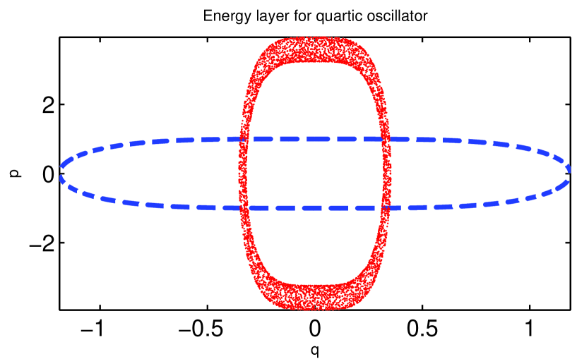
Figure 1: The energy layer for the quartic oscillator $(m=2)$ of the initial microcacnonical ensemble of 5000 points (dashed), with initial energy $E_{0}=0.5$ and $a(t)=1+\epsilon t$, for $\epsilon=1$ and $t=2000$. The layer evolves with time, becoming monotonically thicker.

We shall calculate the width of this layer as a function of time using the nonlinear WKB method adapted for such systems and we will explore the behaviour of the average energy and of the variance of the energy for an initial microcanonical ensemble for large times $t\rightarrow\infty$. If $a(t)$ is a monotonic and unbounded increasing function of time, then both quantities are powers of $a(t)$. In this limit the action first oscillates and finally remains asymptotically constant, but assumes slightly larger value than its initial value. This is an interesting result for time-dependent Hamiltonian systems in a more general context [24, 15]. The distribution function of the final energy will be calculated numerically, but cannot be derived theoretically, unlike the case of the linear oscillator $m=1$, where Robnik, Romanovski and Stöckmann have proven the explicit exact formula for the distribution, which is the arcsine distribution [11, 13].

2 General theory of time-dependent homogeneous power law potential

We consider the Hamilton systems with one degree of freedom in the form quadratic kinetic energy plus a homogeneous power law potential, as defined in equation  (1). Using the nonlinear WKB-like method [8] to the first order approximation for such nonlinear Hamiltonian systems, we have the following general solution,

$$q(t) =a(t)^{-\frac{1}{2m+2}}g\left(\int^{t}_{t_{0}}a(x)^{\frac{1}{m+1}}dx\right),$$

$$p(t) =-\frac{a^{{}^{\prime}}(t)\;(a(t))^{-\frac{1}{2m+2}-1}}{2m+2}g\left(\int^{t}_{t_{0}}a(x)^{\frac{1}{m+1}}dx\right)$$ (2)

$$+(a(t))^{\frac{1}{2m+2}}g^{{}^{\prime}}\left(\int^{t}_{t_{0}}a(x)^{\frac{1}{m+1}}dx\right),$$

where $g$ is the solution of the corresponding time-independent Hamiltonian system with $a(t)=1$ and $g^{{}^{\prime}}$ is its first derivative with respect to time $t$. The function $g$ satisfies the following differential equation,

$$g^{{}^{\prime\prime}}+f(g)=0,$$ (3)

where, $f(g)=dV(g)/dg$. The differential equation (3) admits the first integral, namely the total energy of the oscillator, which is a function of the initial energy $E_{0}$ and the initial phase (canonical angle) $\phi_{0}$ of the oscillator  (1),

$$\quad\frac{(g^{{}^{\prime}}(t))^{2}}{2}+\frac{(g(t))^{2m}}{2m}=c(\phi_{0},E_{0}).$$ (4)

The dependence on $E_{0}$ and $\phi_{0}$ enters through the lower integration limit in equation (2). The expression for the energy of  (1) is

$$E(t) =a(t)^{\frac{1}{m+1}}\left[\frac{\left(g\left(\int^{t}_{t_{0}}a(x)^{\frac{1}{m+1}}dx\right)\right)^{2m}}{2m}+\frac{\left(g^{{}^{\prime}}\left(\int^{t}_{t_{0}}a(x)^{\frac{1}{m+1}}dx\right)\right)^{2}}{2}\right]$$ (5)

$$+\frac{\left[a^{{}^{\prime}}(t)\right]^{2}a(t)^{-\frac{1}{m+1}-2}}{2(2m+2)^{2}}\left[g\left(\int^{t}_{t_{0}}a(x)^{\frac{1}{m}}dx\right)\right]^{2}$$

$$-\frac{a^{{}^{\prime}}(t)a(t)^{-1}}{2m+2}g\left(\int^{t}_{t_{0}}a(x)^{\frac{1}{m+1}}dx\right)g^{{}^{\prime}}\left(\int^{t}_{t_{0}}a(x)^{\frac{1}{m+1}}dx\right).$$

The function $g$ and its derivative $g^{{}^{\prime}}=dg/dt$ are periodic and bounded functions, being the solutions of the time-independent Hamiltonian system (3). Assuming that $a(t)$ is an unbounded monotonically increasing function of time, and also that the $\frac{d\log(a(t))}{dt}$ is a decreasing function of time, we see that if $t\rightarrow\infty$, then $(q(t),p(t))\rightarrow(0,\infty)$. The energy depends on the initial conditions $\phi_{0}$ and $E_{0}$, through the expression in the rectangular brackets, and this is the term which remains non-vanishing for large time $t\rightarrow\infty$,

$$E(t)\simeq c(\phi_{0},E_{0})\;a(t)^{\frac{1}{m+1}}.$$ (6)

After calculating the mean energy and the mean square of the energy, and dropping the decaying terms, we arrive at the following expressions of the leading terms for the average energy and the variance, $Var(E(t))=\langle E(t)^{2}\rangle-\langle E(t)\rangle^{2}$, in the limit $t\rightarrow\infty$,

$$\langle E(t)\rangle\simeq\frac{a(t)^{\frac{1}{m+1}}}{2\pi}\int_{0}^{2\pi}c(\phi_{0},E_{0})d\phi_{0},$$ (7)

$$Var(E(t))\simeq\frac{a(t)^{\frac{2}{m+1}}}{2\pi}\left[\int_{0}^{2\pi}(c(\phi_{0},E_{0}))^{2}d\phi_{0}-\frac{1}{2\pi}\left(\int_{0}^{2\pi}c(\phi_{0},E_{0})d\phi_{0}\right)^{2}\right].$$ (8)

Using the previous expression for the average energy we calculate also the action ratio [15] of the final and initial action. The general formula for the action at the mean energy is,

$$I(\langle E(t)\rangle)=\frac{1}{2\pi}\oint_{H(q,p)=<E(t)>}p\;dq=\frac{2^{\frac{m+1}{2m}}m^{\frac{1}{2m}}\Gamma\left(\frac{1}{2m}\right)}{2m\sqrt{\pi}(a(t))^{\frac{1}{2m}}\Gamma\left(\frac{3m+1}{2m}\right)}\langle E(t)\rangle^{\frac{m+1}{2m}}.$$ (9)

hence the action ratio for large times $t\rightarrow\infty$ is,

$$\frac{I(\langle E_{1}\rangle)}{I(E_{0})}\simeq(a(t_{0}))^{\frac{1}{2m}}\left[\frac{\int_{0}^{2\pi}c(\phi_{0},E_{0})d\phi_{0}}{2\pi E_{0}}\right]^{\frac{m+1}{2m}}=const.$$ (10)

This is an important result, showing that the action ratio remains constant for large times. The numerical empirics shows that it is always slightly larger than its initial value.

3 Examples

In this section we show two examples, the linear oscillator and the quartic oscillator. In the linear oscillator we have exact analytical results for the energy distribution function, as well as for the average energy, the variance and the action ratio [9, 10, 11, 12, 13], but reproduce them here using the more general, although only leading-order, nonlinear WKB-like method [8], now for arbitrarily large times. In the quartic oscillator it is not easy to have explicit theoretical results due the complexity of the Jacobi elliptic functions, but using the numerical technique, for the case with $a(t)=1+\epsilon t$, we calculate and analyze the solutions and show that the general theory of section 2 is correct. For the higher order potentials, $m=3,4,\dots$, we calculate numerically the energy distribution as a function of time (originating from a microcanonical ensemble of initial conditions) and its mean value and the variance, and verify whether they obey the theoretical power laws from section 2.

3.1 Linear oscillator

We consider the Hamiltonian of the linear oscillator in the following form,

$$H(q,p,t)=\frac{p^{2}}{2}+\omega^{2}(t)\frac{q^{2}}{2},$$ (11)

where, $\omega(t)$ is an unbounded monotonically increasing function of time. The general solution using the general nonlinear WKB-like method (which of course is identical to the linear WKB method in the leading order) to the first order approximation is,

$$q(t) =\frac{c_{1}}{\sqrt{\omega(t)}}\sin(c_{2}+\int^{t}_{t_{0}}\omega(x)dx),$$

$$p(t) =c_{1}\sqrt{\omega(t)}\cos(c_{2}+\int^{t}_{t_{0}}\omega(x)dx)-\frac{c_{1}\omega^{{}^{\prime}}(t)}{2(\omega(t))^{\frac{3}{2}}}\sin(c_{2}+\int^{t}_{t_{0}}\omega(x)dx),$$ (12)

where, $c_{1}$ and $c_{2}$ are integration constants. The action-angle variables, for $t=t_{0}$, are

$$q_{0}=\frac{\sqrt{2E_{0}}}{\omega_{0}}\;\sin\phi_{0},\quad\quad p_{0}=\sqrt{2E_{0}}\;\cos\phi_{0},$$ (13)

where, $\omega_{0}=\omega(t_{0})$, $E_{0}$ is the initial energy and $\phi_{0}$ is the initial angle. Using this we get,

$$q(t) =\frac{b_{1}}{\sqrt{\omega(t)}}\left[(b_{2}+\cot\phi_{0})\sin\phi_{0}\;\sin\left(\int^{t}_{t_{0}}\omega(x)dx\right)+\sin\phi_{0}\;\cos\left(\int^{t}_{t_{0}}\omega(x)dx\right)\right],$$

$$p(t) =b_{1}\sqrt{\omega(t)}\left[(b_{2}+\cot\phi_{0})\sin\phi_{0}\;\cos\left(\int^{t}_{t_{0}}\omega(x)dx\right)-\sin\phi_{0}\;\sin\left(\int^{t}_{t_{0}}\omega(x)dx\right)\right]$$

$$-\frac{b_{1}\omega^{{}^{\prime}}(t)}{2(\omega(t))^{\frac{3}{2}}}\left[(b_{2}+\cot\phi_{0})\sin\phi_{0}\;\sin\left(\int^{t}_{t_{0}}\omega(x)dx\right)+\sin\phi_{0}\;\cos\left(\int^{t}_{t_{0}}\omega(x)dx\right)\right].$$

where, $b_{1}=\sqrt{\frac{2E_{0}}{\omega_{0}}}$ and $b_{2}=\frac{\omega^{{}^{\prime}}_{0}}{2\omega_{0}^{2}}$. The average energy after the integration over the $\phi_{0}$ in the interval $\left[0,2\pi\right]$ is,

$$\langle E(t)\rangle =\left(\frac{b_{1}^{2}}{2}+\frac{1}{4}b_{1}^{2}b_{2}^{2}\right)\omega(t)-\frac{b_{1}^{2}b_{2}^{2}(\omega^{{}^{\prime}}(t))^{2}\cos\left(2\int^{t}_{t_{0}}\omega(x)dx\right)}{32\omega^{3}(t)}+\frac{b_{1}^{2}b_{2}^{2}(\omega^{{}^{\prime}}(t))^{2}}{32\omega^{3}(t)}$$ (15)

$$-\frac{b_{1}^{2}b_{2}^{2}\omega^{{}^{\prime}}(t)\sin\left(2\int^{t}_{t_{0}}\omega(x)dx\right)}{8\omega(t)}+\frac{b_{1}^{2}b_{2}(\omega^{{}^{\prime}}(t))^{2}\sin\left(2\int^{t}_{t_{0}}\omega(x)dx\right)}{16\omega^{3}(t)}$$

$$-\frac{b_{1}^{2}b_{2}\omega^{{}^{\prime}}(t)\cos\left(2\int^{t}_{t_{0}}\omega(x)dx\right)}{4\omega(t)}+\frac{b_{1}^{2}(\omega^{{}^{\prime}}(t))^{2}}{16\omega^{3}(t)}.$$

For large time and after a long calculation of the mean squared energy, and dropping the constant and decaying terms, we arrive at the following expressions,

$$\langle E(t)\rangle=\left(\frac{b_{1}^{2}}{2}+\frac{1}{4}b_{1}^{2}b_{2}^{2}\right)\omega(t),$$

$$Var(E(t))=\frac{1}{32}b_{1}^{4}b_{2}^{2}(4+b_{2}^{2})\omega^{2}(t).$$ (16)

While the higher order terms of $\langle E(t)\rangle$ are clearly visible in equation (15), for the variance they are too complex to be presented here, but we only mention that they as a function of time through $\omega(t)$ are constant in the next order, and decay as $1/\omega^{2}(t)$ in the next next order. In manipulations it is necessary to use the computer symbolic calculations.

3.2 Quartic oscillator

We consider the Hamiltonian of the quartic oscillator in the following form,

$$H(q,p,t)=\frac{p^{2}}{2}+a(\lambda)\frac{q^{4}}{4},$$ (17)

where $a(t)$ is an unbounded monotonically increasing function of time. The general solution using the nonlinear WKB-like method [8] to the first order approximation is,

$$q(t) =\frac{\sqrt{2}\;c_{1}}{(a(t))^{\frac{1}{6}}}\;{\rm sn}\left(c_{2}+c_{1}\int^{t}_{t_{0}}(a(x))^{\frac{1}{3}}dx,i\right),$$

$$p(t) =\sqrt{2}\;c_{1}^{2}\;(a(t))^{\frac{1}{6}}\sqrt{1-{\rm sn}^{4}\left(c_{2}+c_{1}\int^{t}_{t_{0}}a(x)^{\frac{1}{3}}dx,i\right)}$$ (18)

$$-\frac{\sqrt{2}\;c_{1}\;a^{{}^{\prime}}(t)\;{\rm sn}\left(c_{2}+c_{1}\int^{t}_{t_{0}}a(x)^{\frac{1}{3}}dx,i\right)}{6\;a(t)^{\frac{7}{6}}},$$

where, $c_{1}$ and $c_{2}$ are integration constants. By $sn$ we denote the Jacobi elliptic function [25]. The initial conditions in terms of the action-angle variables, for $t=t_{0}$, are

$$q_{0}=\sqrt[4]{\frac{4E_{0}}{a_{0}}}\;{\rm sn}\left(\frac{\Gamma^{2}\left(\frac{1}{4}\right)}{2^{\frac{3}{2}}\pi^{\frac{3}{2}}}\phi_{0},i\right),\quad p_{0}=\sqrt{2E_{0}}\sqrt{1-{\rm sn}^{4}\left(\frac{\Gamma^{2}\left(\frac{1}{4}\right)}{2^{\frac{3}{2}}\pi^{\frac{3}{2}}}\phi_{0},i\right)},$$ (19)

where $a_{0}=a(t_{0})$, $E_{0}$ is the initial energy and $\phi_{0}$ is the initial angle. We calculate the constants $c_{1},c_{2}$ as functions of the initial conditions as follows,

$$c_{2}={\rm sn}^{-1}\left(\frac{q_{0}\;a_{0}^{\frac{1}{6}}}{\sqrt{2}\;c_{1}},i\right),$$

$$c_{1}=\sqrt[4]{\frac{E_{0}}{a_{0}^{\frac{1}{3}}}+\frac{\sqrt{2}q_{0}\;p_{0}\;a_{0}^{{}^{\prime}}}{6\;a_{0}^{\frac{4}{3}}}+\frac{q_{0}^{2}\;(a_{0}^{{}^{\prime}})^{2}}{72\;a_{0}^{\frac{7}{3}}}},$$ (20)

and obtain the following expression for the energy

$$E(t)=c_{1}^{4}(a(t))^{\frac{1}{3}}+\frac{c_{1}^{2}(a^{{}^{\prime}}(t))^{2}A^{2}(t)}{36\;(a(t))^{\frac{7}{3}}}-\frac{c_{1}^{3}a^{{}^{\prime}}(t)A(t)\sqrt{1-A^{4}(t)}}{3\;a(t)},$$ (21)

where the function $A(t)$ is the following periodic function,

$$A(t)={\rm sn}\left(c_{2}+c_{1}\int^{t}_{t_{0}}(a(x))^{\frac{1}{3}}dx,i\right).$$ (22)

We cannot analytically calculate the average energy from this expression, unlike in the linear oscillator case. But we see that the leading order term, for $t\gg 1$, is proportional to the power $(a(t))^{\frac{1}{3}}$. The $E^{2}(t)$ has leading order, for $t\gg 1$, proportional to $(a(t))^{\frac{2}{3}}$. For the average energy and the variance, dropping the decaying terms in the limit $t\rightarrow\infty$, we find

$$\langle E(t)\rangle=\frac{a(t)^{\frac{1}{3}}}{2\pi}\int_{0}^{2\pi}c_{1}^{4}d\phi_{0},$$

$$Var(E(t))=\frac{a(t)^{\frac{2}{3}}}{2\pi}\left[\int_{0}^{2\pi}c_{1}^{8}d\phi_{0}-\frac{1}{2\pi}\left(\int_{0}^{2\pi}c_{1}^{4}d\phi_{0}\right)^{2}\right].$$ (23)

The variance is nonzero due to the fact that $\left(\int_{0}^{2\pi}c_{1}^{4}d\phi_{0}\right)^{2}<2\pi\int_{0}^{2\pi}c_{1}^{8}d\phi_{0}$. The higher order constant and decaying terms in equations (3.2) can be easily calculated, but are too complex to be displayed here. In manipulations it is necessary to use the computer symbolic calculations.

The energy distribution for the general family of systems (arbitrary $m$) is difficult to find analytically in a closed formula, except for the linear oscillator $m=1$ [11]. For the model $a(t)=1+\epsilon t$, we have numerically calculated the energy distribution functions and found that for all of them (any $m$) it reminds of the arcsine distribution, as it has two integrable singularity spikes at the minimal and maximal energy, but is distorted in an asymmetric manner. For the quartic oscillator we can find an empirical approximation. Namely, we propose the following rough approximation for the probability density, which is linearly distorted arcsine distribution

$$h(x)=(\frac{1}{\pi}-\frac{\alpha}{2}+\alpha x)x^{-\frac{1}{2}}(1-x)^{-\frac{1}{2}},\quad x\in[0,1].$$ (24)

In the specific numerical example shown in figure 2, we empirically (by best fitting) find $\alpha=0.40175$. We remark that $\alpha=0$ yields the arcsine distribution, which is exact for the linear oscillator for any time dependence $\omega(t)$.

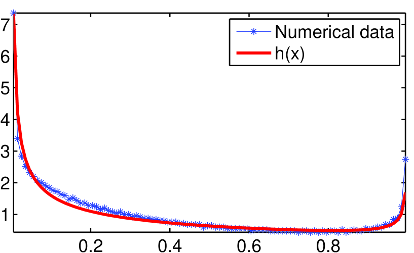
Figure 2: The fitting probability density function $h(x)$ for the quartic oscillator, for $a(t)=1+\epsilon t$, for $\epsilon=1$, $t=2000$ and initial energy $E_{0}=0.5$.

3.3 Higher power law homogeneous potentials

In general it is not easy to calculate the exact expressions of the mean energy and the variance for higher order homogeneous power law potentials, because of the complicated dependence on the initial conditions, due to the complexity of the fundamental solution $g(t)$, entering into the WKB formulae, as described in section 2. Nevertheless, the power laws for the mean energy (7) and the variance (8) are predicted explicitly by the theory, and the proportionality constants can be found empirically (numerically), if needed. We again use the specific model $a(t)=1+\epsilon t$, with $\epsilon=1$, for $m=1,\ldots,6$, and perform the numerical integrations for very large time $t=2000$, using the 8th order symplectic integrator. In the table 1 we present the comparison between the theoretical exponents $1/(m+1)$ for the mean energy, and in the table 2 the exponents $2/(m+1)$ for the variance, with their corresponding numerical values. In addition, in table 3 we calculate the action ratio, using equations (7) and (10).

The exponents for $\langle E(t)\rangle$
m	Numerical value	Theoretical value	Error
1	0,4996481	0.5	3$\cdot 10^{-4}$
2	0.3330987	0.3333333	3$\cdot 10^{-4}$
3	0.249824	0.25	$10^{-4}$
4	0.1998592	0.2	$10^{-4}$
5	0.1665493	0.1666666	$10^{-4}$
6	0.1427567	0.1428571	$10^{-4}$

Table 1: We show the power law exponents for $\langle E(t)\rangle$, whose theoretical value is $1/(m+1)$, as derived in  (7), compared to the numerical results; initial energy $E_{0}=0.5$. The number of points in the initial ensemble is 5000. Time is $t=2000$.

The exponents for $Var(E(t))$
m	Numerical value	Theoretical value	Error
1	0,9992962	1	7$\cdot 10^{-4}$
2	0,6661974	0.6666666	4$\cdot 10^{-4}$
3	0,499648	0.5	3$\cdot 10^{-4}$
4	0,3997184	0.4	2$\cdot 10^{-4}$
5	0,3330986	0.3333332	2$\cdot 10^{-4}$
6	0.2855071	0.2857142	2$\cdot 10^{-4}$

Table 2: We show the power law exponents for $Var(E(t))$, whose theoretical value is $2/(m+1)$, as derived in  (8), compared to the numerical results; initial energy $E_{0}=0.5$. The number of points in the initial ensemble is 5000. Time is $t=2000$.

Values for the action ratio
m	Numerical value	Theoretical value	Error
1	1.0218739	1.0190229	2$\cdot 10^{-3}$
2	1.0110728	1.009601	$10^{-3}$
3	1.0061271	1.0051507	9$\cdot 10^{-4}$
4	1.003837	1.0031063	7$\cdot 10^{-4}$
5	1.0026292	1.002045	6$\cdot 10^{-4}$
6	1.0019214	1.0014258	5$\cdot 10^{-4}$

Table 3: We show the exact value of the action ratio compared to the theoretical, as derived in  (10) for the initial energy $E_{0}=0.5$. The number of points in the initial ensemble is 5000. Time is $t=2000$.

4 Discussion and conclusion

In this work we have analyzed the statistical properties of the one degree of freedom time-dependent Hamilton systems with homogeneous power law potential. We have calculated numerically the energy distribution as a function of time, for large times. Our main interest is in the value of the final average energy, the variance and the action at the final average energy. These are the main parameters describing the energy layer which evolves from the initial microcanonical ensemble. In the case that the dependence on time is monotonic and unbounded, we have calculated the average energy and the variance of the energy using the nonlinear WKB method [8], and derived the power laws observed in the asymptotic limit of large times. In particular, for the adiabatic invariant (action) we have proven that the value becomes constant for very large time but is (empirically) larger than the initial value. The agreement between the theory and the numerics is excellent. Unlike this limit, for small or intermediate times, the analytic expressions become too complicated to be expressed in a closed formula.

To the best of our knowledge this is the first explicit application of the nonlinear WKB-like theory developed in [8]. There are of course many important open questions, namely how to describe other 1D nonlinear Hamilton oscillators, like those studied e.g. in [15], possibly for arbitrary drivings $a(t)$, for which the nonlinear WKB-like method should be generalized, and possibly improved beyond the leading order.

References

References

- [1] Arnold V I 1980 Mathematical Methods of Classical Mechanics (New York: Springer-Verlag)
- [2] Lochak P and Meunier C 1988 Multiphase Averaging for Classical Systems (New York: Springer-Verlag)
- [3] Zaslavsky G M 2007 The Physics of Chaos in Hamiltonian Systems (London: Imperial College Press)
- [4] Ott E 1993 Chaos in Dynamical Systems (Cambridge University Press)
- [5] Chirikov B V 1979 Phys. Rep. 52 263
- [6] Papamikos G and Robnik M 2011 J. Phys. A: Math. Theor. 44 315102
- [7] Papamikos G, Sowden B C and Robnik M 2012 Nonlinear Phenomena in Complex Systems (Minsk) 15 227
- [8] Papamikos G and Robnik M 2012 J. Phys. A: Math. Theor. 45 015206
- [9] Robnik M and Romanovski V G 2006 J. Phys. A: Math. Gen 39 L35-L41
- [10] Robnik M and Romanovski V G 2006 Open Syst. & Infor. Dyn. 13 197-222
- [11] Robnik M, Romanovski V G and Stöckmann H.-J. 2006 J. Phys. A: Math. Gen L551-L554
- [12] Kuzmin A V and Robnik M 2007 Rep. on Math. Phys. 60 69-84
- [13] Robnik M V and Romanovski V G 2008 “Let’s Face Chaos through Nonlinear Dynamics”, Proceedings of the 7th International summer school/conference, Maribor, Slovenia, 2008, AIP Conf. Proc. No. 1076, Eds. M.Robnik and V.G. Romanovski (Melville, N.Y.: American Institute of Physics) 65
- [14] Robnik M and Romanovski V G 2000 J. Phys. A: Math. Gen 33 5093
- [15] Andresas D, Batistić B and Robnik M 2014 Statistical properties of one-dimensional parametrically kicked Hamilton systems, Phys. Rev. E 89 062927; arXiv:1311.1971
- [16] McLachlan R I 1995 SIAM J.Sci.Comput. 16 151-168
- [17] McLachlan R I and Quispel G R W 2002 Acta Numerica, v. 11, p. 341-434, 2002.
- [18] Hairer E, Lubich C and Wanner G 2006 Geometric Numerical Integration, Structure-Preserving Algorithms for Ordinary Differential Equations (Berlin: Springer-Verlag)
- [19] Leimkuhler B and Reich S 2004 Simulating Hamiltonian Dynamics (Cambridge: Cambridge University Press)
- [20] Sanz-Serna J M and Calvo M P 1994 Numerical Hamiltonian Problems (London: Chapman & Hall)
- [21] Shimada M and Yoshida H 1996 Publ. Astron. Soc. Japan 48 147-155
- [22] Yoshida H 1990 Phys. Lett. A 150 262-268
- [23] Yoshida H 1993 Celestial Mechanics and Dynamical Astronomy 56 27-43
- [24] Robnik M 2014 Time dependent linear and nonlinear Hamilton oscillators, edited by A. Pelster and G. Wunner, Selforganization in Complex Systems: The Past, Present, and Future of Synergetics, Proceedings of the International Symposium in Honour of Prof. Hermann Haken, Hanse Institute of Advanced Studies, Delmenhorst, 13-16 November 2012 (Berlin: Springer) to be published
- [25] Olver W F, Lozier W D, Boisvert F R and Clark W C 2010 NIST Handbook of Mathematical Functions, (Cambridge: Cambridge University Press)