Magnetic material in mean-field dynamos driven by small scale helical flows

Abstract

We perform kinematic simulations of dynamo action driven by a helical small scale flow of a conducting fluid in order to deduce mean-field properties of the combined induction action of small scale eddies. We examine two different flow patterns in the style of the G.O. Roberts flow but with a mean vertical component and with internal fixtures that are modelled by regions with vanishing flow. These fixtures represent either rods that lie in the center of individual eddies, or internal dividing walls that provide a separation of the eddies from each other. The fixtures can be made of magnetic material with a relative permeability larger than one which can alter the dynamo behavior. The investigations are motivated by the widely unknown induction effects of the forced helical flow that is used in the core of liquid sodium cooled fast reactors, and from the key role of soft iron impellers in the Von-Kármán-Sodium (VKS) dynamo.

For both examined flow configurations the consideration of magnetic material within the fluid flow causes a reduction of the critical magnetic Reynolds number of up to 25%. The development of the growth-rate in the limit of the largest achievable permeabilities suggests no further significant reduction for even larger values of the permeability.

In order to study the dynamo behavior of systems that consist of tens of thousands of helical cells we resort to the mean-field dynamo theory [1980mfmd.book.....K] in which the action of the small scale flow is parameterized in terms of an $\alpha$- and $\beta$-effect. We compute the relevant elements of the $\alpha$- and the $\beta$-tensor using the so called testfield method. We find a reasonable agreement between the fully resolved models and the corresponding mean-field models for wall or rod materials in the considered range $1\leq\mu_{\rm{r}}\leq 20$. Our results may be used for the development of global large scale models with recirculation flow and realistic boundary conditions.

1 Introduction.

Magnetic fields produced by the flow of a conductive liquid or plasma can be found in almost all cosmic objects. In most cases, this does not apply to liquid metal flows in the laboratory or in industrial applications. The characteristic properties of these flows – namely velocity amplitude, geometric dimension and electrical conductivity – are usually not in the range that allows the occurrence of magnetic self-excitation, so that an experimental confirmation of the fluid flow driven dynamo effect requires an enormous effort. The aforementioned quantities can be combined into a single, dimensionless parameter, the magnetic Reynolds number, which is defined as ${\rm{Rm}}=\mathcal{L}\mathcal{V}/\eta$. Here ${\mathcal{L}}$ is a typical length scale, $\mathcal{V}$ is a typical velocity amplitude, and $\eta$ is the magnetic diffusivity which is the inverse of the product of vacuum permeability and electrical conductivity $\eta=(\mu_{0}\sigma)^{-1}$. In cosmic objects, ${\rm{Rm}}$ is typically huge so that one essential precondition for the occurrence of dynamo action is fulfilled. However, the flow amplitude in terms of ${\rm{Rm}}$ is not the only criterion that describes the ability of a flow field to provide for dynamo action, and magnetic self-excitation is also possible at much smaller $\rm{Rm}$ if the fluid flow has a suitable structure.

Appropriate flows have been utilized, for example, in the three successful fluid flow driven dynamo experiments, the Riga dynamo [2000PhRvL..84.4365G], the Karlsruhe dynamo [2001PhFl...13..561S], and the Von-Kármán-Sodium (VKS) dynamo [2007PhRvL..98d4502M]. Both, Riga dynamo and Karlsruhe dynamo, were based on a screw-like flow pattern, utilizing the fact that helicity is conducive for the occurrence of dynamo action [ISI:000080074100003]. The role of helicity is less obvious for the VKS dynamo with a flow of liquid sodium being driven by two counter-rotating impellers. It has long been known that the mean flow generated by this forcing is suited to drive a dynamo at comparatively low ${\rm{Rm}}$ [1989RSPSA.425..407D]. However, in the experimental implementation at the VKS dynamo, the motor power available to drive the flow is not sufficient to overcome the threshold for the equatorial dipole mode with an azimuthal wavenumber $m=1$. Surprisingly, dynamo action of the axisymmetric dipole mode has yet been found at a rather low magnetic Reynolds number ${\rm{Rm}}\approx 32$ but only if the entire flow driving system, consisting of a disk and eight bended blades (figure 1), is made of soft-iron with a relative permeability in the order of $\mu_{\rm{r}}\approx 60$ [2010NJPh...12c3006V, 2013PhRvE..88a3002M]. A possible explanation for this observation requires the combined effects of the magnetic properties of the soft iron disks [2012NJPh...14e3005G], and helical radial outflows assumed in the vicinity of the impellers between adjacent blades [2007GApFD.101..289P]. These non-axisymmetric distortions of the mean flow can be parameterized by an $\alpha$-effect (figure 1), but so far existing mean-field models of the VKS dynamo are only of limited significance due to a lack of knowledge about the $\alpha$-effect and its interaction with the magnetic material of the impeller systems [2010GApFD.104..249G, 2010PhRvL.104d4503G].

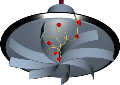
Figure 1: Sketch of an individual impeller that drives the von-Kármán-like flow in the VKS dynamo. The yellow streamline denotes the assumed helical flow between adjacent blades. For dynamo action to occur, both the disk and the blades must be made of soft-iron.

Besides of the relevance for understanding the fundamental physics of geo- and astrophysical magnetic fields, a complementary argument for the development and construction of dynamo experiments originated from considerations on the safe operation of sodium cooled fast reactors [mhdhistory2]. Dynamo action in the cooling system of a sodium fast reactor would likely be dangerous, because the self-induced magnetic field backreacts on the flow according to Lenz’s law. This backreaction might cause an inhomogeneous flow breaking or a pressure drop in the pipe system so that the efficient cooling of the reactor core would be hampered with unknown consequences for the safety of the reactor. The occurrence of dynamo action in a sodium fast reactor can not be excluded a priori because the flow in the core has a sufficiently large flow rate, and the appropriate geometry. In the very core of the reactors the fluid flow is governed by screw-like shaped wires that are wrapped around individual nuclear fuel rods thus forcing the flow to follow a helical path around each rod (figure 2a).

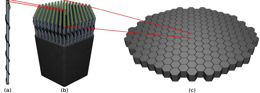
Figure 2: Idealized composition of the core of a sodium fast reactor; from left to right: (a) nuclear fuel rod surrounded by a helical shaped spacer forcing the flow on a helical path; (b) assembly of bundled fuel rods; (c) array of assemblies, forming the core of a liquid metal cooled fast reactor. Note that the figure shows an idealized system. In real systems, there are still additional elements with breeding material and control rods.

These fuel rods are bundled into so called assemblies which may consist of up to a few hundreds of fuel rods (figure 2b), and the whole reactor core is composed of a few hundreds of these assemblies (figure 2c). In operation, this setup is flushed with liquid sodium thereby forming a helical flow field that is reminiscent of the flow used in the Karlsruhe dynamo (except the mean vertical component).

Actually, early estimations by bevir bevir and pierson pierson as well as more recent experimental and numerical studies [1995maghyd...31.4..382P, 1999JFM...382..137P, 2000JFM...403..263A] show no conclusive evidence for the occurrence of dynamo action in the core of a fast reactor. On the other hand it has been argued by thesis_soto thesis_soto that the parameter regime reached by the French fast breeder reactor Superphenix is well within the range that allows for dynamo action if some magnetic material is introduced into the container thesis_sotosee p. 104, Fig III.32 in. So far, the problem of magnetic material in the core of a sodium fast reactor is merely academic, because state of the art reactors mainly utilize austenitic steels inside the core. However, in recent years, the application of Oxide Dispersion Strengthened (ODS) ferritic/martensitic alloys with a relative permeability $\mu_{\rm{r}}\gg 1$ has increasingly been discussed because these alloys have a lower sensitivity for nuclear radiation [2012JNuM..428....6D].

The dramatic influence of magnetic properties on the induction process, as observed at the VKS dynamo, motivated the present study, in which we examine complex interactions of helical flow fields with magnetic internals. Since the flow conditions in a sodium fast reactor are far too complex to be modeled in direct numerical simulations, we resort to the mean-field dynamo theory, which allows the development of models that are numerically much easier to handle. In order to consider the specific effects of a spatially varying permeability distribution we extend the original mean-field concept to the case of non-uniform material properties. The extension is straightforward and allows to take into account complex periodic patterns with magnetic properties in terms of standard mean-field coefficients like the $\alpha$- and $\beta$-effect. For the estimation of the mean-field coefficients we perform kinematic simulations of electromagnetic induction generated by idealized helical flow fields that are reminiscent of the conditions in sodium fast reactors. We consider two paradigmatic configurations with either a helical flow subdivided by internal walls, or a flow following a helical path around solid rods, respectively. The first model follows the heuristic approach of pierson pierson in which the screw-like vortex represents the mean flow within an assembly of nuclear fuel rods. In a very broad sense, this model can also serve as an approach for the flow field between the blades in the VKS dynamo. The second model goes back to the work of 2002NPGeo…9..171R 2002NPGeo…9..171R,2002MHD….38…41R on the kinematic theory of the Karlsruhe dynamo. In the present study, in which we assume a vertical mean flow, this type of flow field is suited to the conditions within an assembly of fuel rods in the core of a sodium fast reactor.

We start with the analysis of the induction action of the fully resolved velocity field, from which we determine the mean-field coefficients using the testfield method [2005AN....326..245S, 2007GApFD.101...81S]. In a second step we use the $\alpha$- and $\beta$-coefficients as an input for mean field dynamo simulations in order to prove that mean-field models are capable to reproduce the growth-rate and principle field structure of the fully resolved model by requiring much less computational efforts. For flow systems comprising a total of some tens of thousands of individual helical cells (figure 2), the use of a well-proven mean-field method is considered the only viable way to study dynamo problems. The present paper is mainly intended to establish and validate the necessary methodology. The possible application to specific reactor cores will need much more information on geometric details and material properties, and must therefore be left for future work.

2 Mean-field dynamo theory and the testfield method

2.1 Outline of mean-field theory

In the following, the magnetic flux density is denoted by $B$ and the velocity field by $U$. The magnetic diffusivity is defined by $\eta=(\mu\sigma)^{-1}$ with the electrical conductivity $\sigma$ and the permeability $\mu$ which are assumed, for the moment, to be constant. The temporal development of the magnetic flux density in the presence of an electrically conductive liquid that moves according to the velocity field $U$ is determined by the induction equation:

$$\frac{\partial\mbox{\boldmath$B$}}{\partial t}=\nabla\times\left(\mbox{\boldmath$U$}\times\mbox{\boldmath$B$}-\eta\nabla\times{\mbox{\boldmath$B$}}\right).$$ (1)

Additionally, $B$ must obey the divergence-free condition, $\nabla\cdot\mbox{\boldmath$B$}=0$. In case of a prescribed (stationary) velocity field, equation  (1) is a linear problem which, in principle, can be solved with the Ansatz

$$\mbox{\boldmath$B$}(\mbox{\boldmath$r$},t)=\mbox{\boldmath$B$}_{0}(\mbox{\boldmath$r$})e^{\lambda t}.$$ (2)

In general $\lambda$ is a complex quantity $\lambda=\kappa+i\omega$ where $\kappa$ denotes the growth-rate and $\omega$ denotes an oscillation- or drift-frequency. A dynamo solution is obtained if the magnetic field amplitude $|\mbox{\boldmath$B$}|$ grows exponentially $\propto e^{\kappa t}$ with a growth-rate $\kappa>0$.

Even though the linear approach is a severe simplification that neglects the backreaction of the field on the flow, equation (1) can be solved analytically only for very few cases. In particular for complicated velocity fields with small scale structures, equation (1) must be solved numerically. A possibility to draw further conclusions on the ability of a velocity field to drive a dynamo is provided by the mean-field dynamo theory developed by 1980mfmd.book…..K 1980mfmd.book…..K. The mean-field dynamo theory essentially deals with the behavior of the large scale field and treats the induction effects of a small scale flow in terms of the so called $\alpha$-effect. The basic principle of the mean-field approach is a splitting of magnetic field and velocity field assuming that the properties of the whole system can be described essentially by two scales, a mean, large scale part ($\overline{\mbox{\boldmath$B$}}$ and $\overline{\mbox{\boldmath$U$}}$) and a small scale fluctuation ($b$ and $u$):

$$B = \overline{\mbox{\boldmath$B$}}+\mbox{\boldmath$b$},$$ (3)

$$U = \overline{\mbox{\boldmath$U$}}+\mbox{\boldmath$u$}.$$ (4)

Inserting (3) and (4) into (1) yields an induction equation for the mean-field $\overline{\mbox{\boldmath$B$}}$:

$$\frac{\partial\overline{\mbox{\boldmath$B$}}}{\partial t}=\nabla\times\left(\overline{\mbox{\boldmath$U$}}\times\overline{\mbox{\boldmath$B$}}+\overline{\mbox{\boldmath$u$}\times\mbox{\boldmath$b$}}-\eta\nabla\times\overline{\mbox{\boldmath$B$}}\right),$$ (5)

while the induction equation for the corresponding small scale field $b$ reads:

$$\frac{\partial\mbox{\boldmath$b$}}{\partial t}=\nabla\times\left(\overline{\mbox{\boldmath$U$}}\!\times\!\mbox{\boldmath$b$}+\mbox{\boldmath$u$}\!\times\!\overline{\mbox{\boldmath$B$}}+\left(\mbox{\boldmath$u$}\!\times\!\mbox{\boldmath$b$}-\overline{\mbox{\boldmath$u$}\!\times\!\mbox{\boldmath$b$}}\right)-\eta\nabla\!\times\!\mbox{\boldmath$b$}\right).$$ (6)

Furthermore, the mean-field as well as the small scale field must obey $\nabla\cdot\overline{\mbox{\boldmath$B$}}\!=\!0$ and $\nabla\cdot\mbox{\boldmath$b$}\!=\!0$. The mean-field induction equation (5) contains an additional source term, $\boldmath{\mathcal{E}{\mbox{\boldmath$$}}}\!=\!\overline{\mbox{\boldmath$u$}\!\times\!\mbox{\boldmath$b$}}$, called the mean electromotive force (EMF). In the kinematic approximation, $\boldmath{\mathcal{E}{\mbox{\boldmath$$}}}$ is linear and homogeneous in $\overline{\mbox{\boldmath$B$}}$, and, under the assumption that the variations of $\overline{\mbox{\boldmath$B$}}$ around a given point are small, $\boldmath{\mathcal{E}\mbox{\boldmath$$}}$ can be represented by the first terms of a Taylor expansion:

$${\mathcal{E}}_{i}=\alpha_{ij}B_{j}+\beta_{ijk}\frac{\partial B_{j}}{\partial x_{k}}.$$ (7)

Here $\alpha_{ij}$ and $\beta_{ijk}$ are tensors of second and third rank, respectively. The diagonal components $\alpha_{ii}$ give rise to an electromotive force parallel to the mean magnetic field and therefore may be responsible for dynamo action. For isotropic turbulence, the contribution proportional to the mean-field gradients simplifies to $\beta\epsilon_{ijk}\partial B_{j}/\partial x_{k}$ (with the Levi-Civita tensor $\epsilon_{ijk}$), so that this term behaves similar to a diffusive contribution. However, in our setup we have a strong anisotropy between vertical and horizontal coordinates, so that we refer to another expression for the electromotive force, that is based on elementary symmetry properties of flow and field [1980mfmd.book.....K]:

$$\mathcal{E} = -\alpha_{\perp}\overline{\mbox{\boldmath$B$}}-(\alpha_{\parallel}\!-\!\alpha_{\perp})(\hat{\mbox{\boldmath$z$}}\!\cdot\!\overline{\mbox{\boldmath$B$}})\hat{\mbox{\boldmath$z$}}-\gamma\hat{\mbox{\boldmath$z$}}\!\times\!\overline{\mbox{\boldmath$B$}}-\beta_{\perp}\nabla\!\times\!\overline{\mbox{\boldmath$B$}}-(\beta_{\parallel}\!-\!\beta_{\perp})(\hat{\mbox{\boldmath$z$}}\!\cdot\!(\nabla\!\times\!\overline{\mbox{\boldmath$B$}}))\hat{\mbox{\boldmath$z$}}$$ (8)

$$-\widetilde{\beta}\hat{\mbox{\boldmath$z$}}\!\times\!(\nabla(\hat{\mbox{\boldmath$z$}}\!\cdot\!\overline{\mbox{\boldmath$B$}})+(\hat{\mbox{\boldmath$z$}}\!\cdot\!\nabla)\overline{\mbox{\boldmath$B$}})-\delta_{1}\nabla(\hat{\mbox{\boldmath$z$}}\!\cdot\!\overline{\mbox{\boldmath$B$}})-\delta_{2}(\hat{\mbox{\boldmath$z$}}\!\cdot\!\nabla)\overline{\mbox{\boldmath$B$}}-\delta_{3}(\hat{\mbox{\boldmath$z$}}\!\cdot\!\nabla(\hat{\mbox{\boldmath$z$}}\!\cdot\!\overline{\mbox{\boldmath$B$}}))\hat{\mbox{\boldmath$z$}}.$$

Here, a mean flow is assumed along the vertical direction which is labeled by $\hat{\mbox{\boldmath$z$}}$ in a Cartesian system. The subscript $\parallel$ denotes quantities that are parallel to this vertical direction whereas the subscript $\perp$ denotes quantities that are oriented in the horizontal plane ($xy$-plane). In equation (8), $\alpha_{\perp}$ and $\alpha_{\parallel}$ give rise to a current parallel to the mean magnetic field and, hence, can be responsible for dynamo action. These coefficients correspond to the diagonal elements of the $\alpha$-tensor, and anisotropic effects arising from properties of the small scale velocity field result in different contributions from the horizontal part $\alpha_{\perp}$ (that generates a current in the $xy$-plane) and the vertical part $\alpha_{\parallel}$ (that generates a current along the $z$-axis). In the same way, $\beta_{\perp}$ and $\beta_{\parallel}$ can be interpreted as anisotropic contributions to the magnetic diffusivity. The coefficient $\gamma$ is related to the antisymmetric part of the $\alpha$-tensor and describes an additional advection of the mean-field in the direction of the mean flow. The remaining coefficients $\widetilde{\beta}$ and $\delta_{i}$ are related to the gradient tensor of the magnetic field and have no simple analogy. A more detailed derivation of equation (8) and a discussion about the mean-field coefficients $\alpha_{\perp},\alpha_{\parallel},\beta_{\perp},\beta_{\parallel},\widetilde{\beta},\delta_{i}$ are given in the textbook of 1980mfmd.book…..K 1980mfmd.book…..K.

In the following, we only consider flow fields that do not depend on $z$ and that are periodic in the $xy$-plane. All mean quantities are defined as horizontal averages, i.e., they do not depend on $x$ or $y$. Consequently, most of the coefficients and all terms proportional to mean-field gradients in $x$ and $y$ vanish so that (8) can be significantly simplified:

$$\mbox{\boldmath$\mathcal{E}$}=-\alpha_{\perp}(\overline{\mbox{\boldmath$B$}}-(\hat{\mbox{\boldmath$z$}}\cdot\overline{\mbox{\boldmath$B$}})\hat{\mbox{\boldmath$z$}})-(\beta_{\perp}+\widetilde{\beta})\hat{\mbox{\boldmath$z$}}\times\frac{d\overline{\mbox{\boldmath$B$}}}{dz}-\gamma{\hat{\mbox{\boldmath$z$}}}\times\overline{\mbox{\boldmath$B$}}-\delta_{2}\frac{d\overline{\mbox{\boldmath$B$}}}{dz}.$$ (9)

Note, that due to the constant velocity along $z$ and the vanishing horizontal derivatives of the mean-field, all contributions labeled with $\parallel$ can be dropped and only two terms $\propto\partial\overline{\mbox{\boldmath$B$}}/\partial z$ survive. Furthermore, the effects corresponding to $\beta_{\perp}$ and $\widetilde{\beta}$ cannot be distinguished any more and are subsumed into one common coefficient $\beta=\beta_{\perp}+\widetilde{\beta}$ [2003PhRvE..67b6401R].

The tensor coefficients appearing in (7) can be related to the more descriptive notation used in (9) giving the following relations:

$$\alpha_{xx}= \quad\alpha_{yy} =-\alpha_{\perp},$$

$$\alpha_{xy}= -\alpha_{yx} =\quad\gamma,$$ (10)

$$\beta_{xyz}= -\beta_{yxz} =-(\beta_{\perp}+\widetilde{\beta})=-\beta,$$

$$\beta_{xxz}= \quad\beta_{yyz} =-\delta_{2}.$$

These relations reflect the horizontal isotropy in our models and allow a simplification of the problem since only four coefficients must be determined in order to establish a consistent mean-field model.

2.2 Testfield method

The test field method developed in 2005AN….326..245S provides a powerful tool to compute the coefficients $\alpha_{ij}$ and $\beta_{ijk}$ from different realizations of the electromotive force that are obtained from externally applied, linearly independent mean-fields. Here, we restrict ourselves to the kinematic case with a stationary velocity field although the method can also be applied to fully non-linear magnetohydrodynamic systems where $U$ is computed by solving the Navier-Stokes equation.

The fluctuating velocity field is computed from the full velocity field $U$ by

$$\mbox{\boldmath$u$}=\mbox{\boldmath$U$}-\overline{\mbox{\boldmath$U$}}$$ (11)

with $\overline{\mbox{\boldmath$U$}}$ being the horizontal average of $U$. The small scale magnetic field $b$ is computed numerically by solving equation (6) with $\overline{\mbox{\boldmath$B$}}$ defined as an external steady field, the so called testfield. Then the electromotive force is computed directly by correlating small scale flow with the small scale field and subsequently performing a horizontal averaging: $\boldmath{\mathcal{E}}=\overline{\mbox{\boldmath$u$}\times\mbox{\boldmath$b$}}$. The combination of different realizations of $\boldmath{\mathcal{E}}\mbox{\boldmath$$}$ obtained from different, linearly independent testfields with (7) yields a linear system of equations whose solution gives the desired mean-field coefficients. In principle, only minor preconditions for the testfields must be considered. In order to calculate mean-field coefficients that are consistent with the structure of the large scale field obtained from the fully resolved model it is necessary to consider the scale dependence of the mean-field coefficients [2008A&A...482..739B]. Around the onset of dynamo action the vertical dependence of the large scale field in our systems is $\propto\cos(z)$ (or $\propto\sin(z)$) which is exactly the vertical structure that we imply to the testfields. Because of the horizontal isotropy of our system, we define two testfields oriented in the horizontal plane parallel to $\hat{\mbox{\boldmath$y$}}$:

$$\overline{\mbox{\boldmath$B$}}_{1}=\cos(z)\hat{\mbox{\boldmath$y$}}\mbox{ and }\overline{\mbox{\boldmath$B$}}_{2}=\sin(z)\hat{\mbox{\boldmath$y$}}.$$ (12)

With this definition we obtain four equations with four unknown mean field coefficients $\alpha_{yy},\alpha_{xy},\beta_{yyz},\beta_{xyz}$ which read:

$${\alpha}_{yy} = \overline{\mathcal{E}}_{1,y}(z)\cos(z)+\overline{\mathcal{E}}_{2,y}(z)\sin(z),$$ (13)

$${\beta}_{xyz} = -\left(\overline{\mathcal{E}}_{1,x}(z)\sin(z)-\overline{\mathcal{E}}_{2,x}(z)\cos(z)\right),$$ (14)

$$\alpha_{xy} = \overline{\mathcal{E}}_{1,x}(z)\cos(z)+\overline{\mathcal{E}}_{2,x}(z)\sin(z),$$ (15)

$$\beta_{yyz} = -\left(\overline{\mathcal{E}}_{1,y}(z)\sin(z)-\overline{\mathcal{E}}_{2,y}(z)\cos(z)\right).$$ (16)

Here $\mathcal{E}_{1,2,x,y}$ denote the horizontal components of the electromotive force obtained with the testfields $\overline{\mbox{\boldmath$B$}}_{1,2}$. The remaining coefficients $\alpha_{xx},\alpha_{yx},\beta_{yxz}$ and $\beta_{xxz}$ can, in principle, be calculated with similar equations involving $\boldmath{\mathcal{E}}{\mbox{\boldmath$$}}$ obtained from $\overline{\mbox{\boldmath$B$}}_{3}=\cos(z)\hat{\mbox{\boldmath$x$}}$ and $\overline{\mbox{\boldmath$B$}}_{4}=\sin(z)\hat{\mbox{\boldmath$x$}}$ which requires the numerical solution of two further partial differential equations for the corresponding $b$. For test purposes we have additionally performed these calculations and verified that the isotropy conditions given by (10) are met in the simulations.

3 Flow models and permeability distribution

3.1 Velocity field

In the present study we examine two different flow models: In model A we assume a flow consisting of various helical eddies that are separated by walls (left panel in figure 3). This flow definition resembles the Roberts-flow [1970RSPTA.266..535R, 1972RSPTA.271..411R] but comprises a separating region between each cell quite similar to the model examined by 2005AN….326..250S 2005AN….326..250S. In contrast to the Roberts-flow, the flow in our model has the same orientation (left-handed) in every cell. However, in combination with a uniform vertical flow, each cell provides the same helicity as it is also the case for the Roberts flow. We further allow for a variation of the relative permeability assuming that magnetic material is used to guide the flow along the vertical direction. Following the idea of pierson, the helical flow within one cell represents the mean flow within one assembly of nuclear fuel rods ignoring the even smaller scale flow around individual rods.

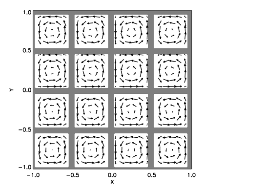
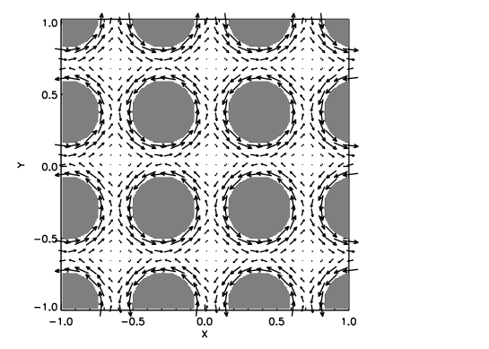
Figure 3: Flow pattern for model A (left panel) and model B (right panel). The gray shaded regions represent walls (model A, left) or rods (model B, right) and the arrows denote the horizontal flow. The vertical flow is constant within each cell and vanishes in the wall/rod regions. The fluid permeability is $\mu_{\rm{r}}=1$ and the wall/rod permeability is varied in the range $1\leq\mu_{\rm{r}}\leq 20$.

The flow with amplitude $u_{0}$ in one individual cell of size $D$ is given by

$$u_{x} = \quad\!u_{0}\sin\left(\pi\frac{x-x_{0}}{D}\right)\cos\left(\pi\frac{y-y_{0}}{D}\right),$$

$$u_{y} = -u_{0}\cos\left(\pi\frac{x-x_{0}}{D}\right)\sin\left(\pi\frac{y-y_{0}}{D}\right),$$ (17)

$$u_{z} = \quad\!u_{0},$$

where $x_{0}$ and $y_{0}$ represent the coordinates of the cell center in the horizontal plane. The total velocity field is a superimposition of $N$ cells (each using (17)) which additionally considers the wall regions by setting $v_{x}=v_{y}=v_{z}=0$ there. The thickness of the walls is defined as $d=2/(6\sqrt{N})$ with $N$ the number of helical cells. The definition of the wall thickness ensures that the relation of cell size to wall thickness is constant when increasing the number of cells. The specific value is chosen so that the number of grid points representing a wall is sufficient to numerically resolve the effects of the permeability transition of the fluid-wall interface. We used four different realizations with $N=4,16,64$ and $256$ cells arranged in a squared pattern, however, most simulations have been performed using the setup shown in the left panel of figure 3 where $16$ cells in a horizontal plane are displayed.

The second approach (model B, see right panel in figure 3) uses a more detailed picture of the flow conditions within a single assembly. The model is based on the so called spin generator flow that has been utilized for the simulation of the Karlsruhe Dynamo [2002NPGeo...9..171R, 2002MHD....38...41R, 2003PhRvE..67b6401R]. A detailed numerical model of the flow in a hexagonal assembly consisting of seven fuel rods including a wire wrap surrounding each rod can be found in gajapathy gajapathy where the Navier-Stokes equation is solved numerically and turbulence effects are included in terms of a standard $k-\epsilon$ model. Here, we use a simplified flow field roughly in accordance with the model of 2002MHD….38…41R 2002MHD….38…41R,2002NPGeo…9..171R by assuming a circular flow around a central rod superimposed with a constant vertical flow. The flow around a single rod is defined as

$$u_{x} = -\frac{1}{2}u_{0}\frac{y-y_{0}}{\sqrt{(x-x_{0})^{2}+(y-y_{0})^{2}}}\left(1+\cos\!\left(\pi\frac{\sqrt{(x-x_{0})^{2}+(y-y_{0})^{2}}-R}{D}\right)\!\right)$$

$$u_{y} = \frac{1}{2}u_{0}\frac{x-x_{0}}{\sqrt{(x-x_{0})^{2}+(y-y_{0})^{2}}}\left(1+\cos\!\left(\pi\frac{\sqrt{(x-x_{0})^{2}+(y-y_{0})^{2}}-R}{D}\right)\!\right)$$ (18)

$$u_{z} = u_{0}$$

where $(x_{0},y_{0})$ is the center of a rod, $R$ is the radius of the rod and $D$ is the distance between two adjacent rods (see right panel of figure 3). We have performed simulations with $9$ and $25$ rods regularly distributed in the horizontal plane.

Note, that all helical flow cells in both models are left-handed, so that the helicity provided by each cell has the same sign. Furthermore, the global dimensions of the computational domain remain the same, independent of the number of cells, so that an increasing number of cells or rods goes along with a smaller scale of the fluctuating flow component and, thus, an increased separation between large scale and small scale flow. Horizontal isotropy is preserved by applying a quadratical configuration (identical linear extensions and identical resolution) and periodic boundaries. The vertical extent of the computational domain is $z\in[0;2\pi]$ with periodic boundaries as well.

The Cartesian geometry is different from the hexagonal pattern of realistic assemblies. However, we believe that for the development of the methodology, the numerically much easier to handle Cartesian geometry is more advantageous without exhibiting excessive deviations from the realistic case.

In order to characterize the amplitude of the flow we define a local magnetic Reynolds number that is based on the flow amplitude $u_{0}$, the “normal” magnetic diffusivity $\eta=(\mu_{0}\sigma)^{-1}$ and the size $D$ of a single eddy (model A) or the distance between two adjacent rods (model B):

$${\rm{Rm}}_{\rm{loc}}=\frac{u_{0}D}{\eta}.$$ (19)

3.2 Permeability distribution

The standard mean-field approach developed in 1980mfmd.book…..K is not intended to consider a spatially varying (“fluctuating”) permeability which can easily be seen taking the case ${\rm{Rm}}=0$. Then the EMF must vanish, ${\boldmath{\mathcal{E}}{\mbox{\boldmath$$}}}=0$ (since $\mbox{\boldmath$u$}=0$) and thus all mean-field coefficients vanish independently from the actual distribution of $\mu_{\rm{r}}$. Our modification starts with the induction equation with a non-uniform permeability distribution $\mu_{\rm{r}}=\mu_{\rm{r}}(\mbox{\boldmath$r$})$, which reads

$$\frac{\partial\mbox{\boldmath$B$}}{\partial t}=\nabla\times\left(\mbox{\boldmath$U$}\times\mbox{\boldmath$B$}-\eta\nabla\times\frac{\mbox{\boldmath$B$}}{\mu_{\rm{r}}}\right).$$ (20)

Using standard vector relations and $\nabla\cdot\overline{\mbox{\boldmath$B$}}=0$ we rewrite (20) in the form

$$\frac{\partial\mbox{\boldmath$B$}}{\partial t}=\nabla\times\left(\mbox{\boldmath$U$}\times\mbox{\boldmath$B$}+{\widetilde{\eta}}\frac{\nabla\mu_{\rm{r}}}{\mu_{\rm{r}}}\times{\mbox{\boldmath$B$}}-\widetilde{{\eta}}\,\nabla\times\mbox{\boldmath$B$}\right)$$ (21)

with $\widetilde{\eta}=\widetilde{\eta}(\mbox{\boldmath$r$})=\eta/\mu_{\rm{r}}(\mbox{\boldmath$r$})$. The modified induction equation (21) exhibits an additional, not necessarily divergence-free, velocity-like term, sometimes called paramagnetic pumping [2003PhRvE..67e6309D]:

$$\widetilde{\mbox{\boldmath$u$}}(\mbox{\boldmath$r$})=\widetilde{\eta}\frac{\nabla\mu_{\rm{r}}}{\mu_{\rm{r}}(\mbox{\boldmath$r$})}.$$ (22)

We define a modified velocity field $\widetilde{\mbox{\boldmath$U$}}=\mbox{\boldmath$U$}+\widetilde{\mbox{\boldmath$u$}}$ which is now the velocity field that has to be split up into mean part and fluctuating part when applied in the testfield method. Note, that the introduction of the pumping velocity $\widetilde{\mbox{\boldmath$u$}}$ provides a non-vanishing fluctuating velocity contribution even in case of a vanishing fluid flow (i.e. when $u_{0}=0$). In our model, we first define a permeability distribution, from which we compute the corresponding pumping velocity $\widetilde{\mbox{\boldmath$u$}}$ using a simple finite difference discretisation. In the fluid regions (where $u_{z}\neq 0$), the permeability distribution takes the value $\mu_{\rm{r}}=1$, and $\mu_{\rm{r}}$ is set to a fixed value $\neq 1$ in the remaining regions (where $u_{z}=0$, indicated by the grey shaded areas in figure 3). In order to avoid the discontinuity at the fluid-solid body transition, which would lead to an amplitude for the pumping velocity that depends on the grid-resolution, we smoothed the discontinuity at the fluid-solid body interface by assuming some sinusoidal distribution with a fixed length-scale that is independent of the grid resolution.

4 Results

In this section, we will apply the test field method to the two geometric models A and B, first without and then with consideration of magnetic materials. In each case we will validate the correspondence of the dynamo action of the fully resolved and the derived mean-field models.

4.1 Homogeneous case ($\mu_{\rm{r}}=1$)

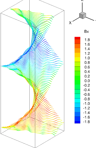
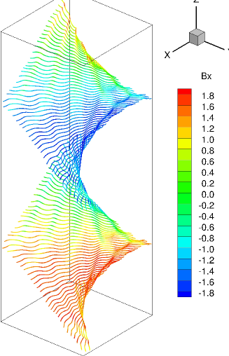
Figure 4: Streamlines of the magnetic field slightly above the dynamo threshold (left: model A with 16 cells, ${\rm{Rm}}_{\rm{loc}}=5.2$, right: model B with 25 rods, ${\rm{Rm}}_{\rm{loc}}=1.6$) The color coding denotes the $x-$ component of the magnetic field. Note the different orientation sense of the helical structure. The undulations reflect the small scale field components.

The typical structure of the magnetic field just above the dynamo threshold is shown in Figure 4. The field geometry is remarkably similar for both models and essentially describes a large scale helical pattern dominated by the horizontal components. The small scale field is visible in terms of little undulations on top of the large scale structure.

4.1.1 ${\alpha}$– and ${\beta}$– effect

We start with a uniform permeability distribution with $\mu_{\rm{r}}=1$ for both the fluid and the solid internals. The resulting $\alpha$-effect is qualitatively in accordance with the results from 2002NPGeo…9..171R 2002NPGeo…9..171R,2002MHD….38…41R for $\alpha$ in case of an ideal Roberts flow. Similarly, we write for the $\alpha$-coefficient

$$\alpha_{\perp}=K\frac{\eta}{D}{\rm{Rm}}_{\rm{loc}}^{2}\Phi({\rm{Rm}}_{\rm{loc}})$$ (23)

with a constant $K$ ($K\approx 0.026$ for model A and $K\approx 0.066$ for model B) and a non-analytic function $\Phi$ that only depends on ${\rm{Rm}}_{\rm{loc}}$. Figure 5 shows the behavior of $\Phi$ versus the flow amplitude ${\rm{Rm}}_{\rm{loc}}$ for three different realizations of model A (with $4,16$ and $64$ helical cells, left panel) and for two realizations of model B ($9$ and $25$ rods, right panel).

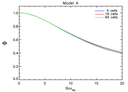
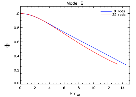
Figure 5: $\Phi=\alpha_{\perp}D/(K\eta{\rm{Rm}}_{\rm{loc}}^{2})$ versus ${\rm{Rm}}_{\rm{loc}}$ for different configurations characterized by an increasing number of helical cells. Left: flow model A. Right: flow model B.

Note, that the normalization factor $K$ is universal for each model and does not depend on the cell size $D$. Qualitatively, the behavior of the function $\Phi$ is similar for both flow models. $\Phi$ approaches its maximum value for ${\rm{Rm}}_{\rm{loc}}\rightarrow 0$ and decreases monotonically with increasing ${\rm{Rm}}_{\rm{loc}}$, so that, presumably, $\Phi$ will asymptotically approach zero for very large flow amplitudes. Here, we are limited to ${\rm{Rm}}_{\rm{loc}}\mathrel{\mathchoice{\vbox{\offinterlineskip\halign{\hfil$\displaystyle#$\hfil\cr<\cr\sim\cr}}}{\vbox{\offinterlineskip\halign{\hfil$\textstyle#$\hfil\cr<\cr\sim\cr}}}{\vbox{\offinterlineskip\halign{\hfil$\scriptstyle#$\hfil\cr<\cr\sim\cr}}}{\vbox{\offinterlineskip\halign{\hfil$\scriptscriptstyle#$\hfil\cr<\cr\sim\cr}}}}20$ for model A and to ${\rm{Rm}}_{\rm{loc}}\mathrel{\mathchoice{\vbox{\offinterlineskip\halign{\hfil$\displaystyle#$\hfil\cr<\cr\sim\cr}}}{\vbox{\offinterlineskip\halign{\hfil$\textstyle#$\hfil\cr<\cr\sim\cr}}}{\vbox{\offinterlineskip\halign{\hfil$\scriptstyle#$\hfil\cr<\cr\sim\cr}}}{\vbox{\offinterlineskip\halign{\hfil$\scriptscriptstyle#$\hfil\cr<\cr\sim\cr}}}}14$ for model B because above these values the occurrence of small scale dynamo action with exponentially growing small scale field prevents a reliable estimation oft the mean-field coefficients. The onset of small scale dynamo action occurs at smaller ${\rm{Rm}}_{\rm{loc}}$ for a larger number of cells, so that the models with the largest $N$ determine the largest achievable ${\rm{Rm}}_{\rm{loc}}$. Nevertheless, both models are already highly overcritical at this $\rm{Rm}_{\rm{loc}}$ so we are still able to discuss the behavior around the onset of dynamo action (which is of main interest in the present context).

Regarding the coefficient $\beta$, we find significant differences between both models (figure 6). To our knowledge, no analytic expressions for $\beta$ beyond the second order correlation approximation (SOCA), in which $\mbox{\boldmath$u$}\times\mbox{\boldmath$b$}-\overline{\mbox{\boldmath$u$}\times\mbox{\boldmath$b$}}=0$ is assumed, are available in the literature (see, e.g., tilgner01 for an expression for $\beta$ using SOCA). The restricted validity of SOCA is shown in 2008A&A…482..739B where mean-field coefficients obtained from the test-field method with and without SOCA are compared. Since in our model the preconditions for SOCA are not met, we refrain from a similar analysis. Surprisingly, we do not observe any dependency on the cell size for model A and only a weak dependence in case of model B. Thus, the $\beta$-effect mainly depends on ${\rm{Rm}}_{\rm{loc}}$ and is independent of the characteristic wave number of the small scale flow (at least within the rather restricted range of flow scales that has been examined for this study).

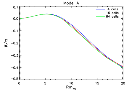
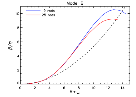
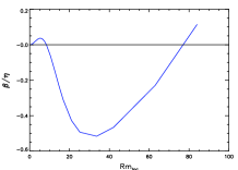
Figure 6: $\beta$ versus ${\rm{Rm}}_{\rm{loc}}$ for different configurations of flow model A and B. (left: model A, right: model B). The insert plot in the left panel shows the behavior of $\beta$ for very large ${\rm{Rm}}_{\rm{loc}}$ (computed from the model with $4$ helical cells). The dashed black curve in the right panel shows a fitting function $\sim 0.062{\rm{Rm}}_{\rm{loc}}^{2}$ (fitted to the red curve for ${\rm{Rm}}_{\rm{loc}}\mathrel{\mathchoice{\vbox{\offinterlineskip\halign{\hfil$\displaystyle#$\hfil\cr<\cr\sim\cr}}}{\vbox{\offinterlineskip\halign{\hfil$\textstyle#$\hfil\cr<\cr\sim\cr}}}{\vbox{\offinterlineskip\halign{\hfil$\scriptstyle#$\hfil\cr<\cr\sim\cr}}}{\vbox{\offinterlineskip\halign{\hfil$\scriptscriptstyle#$\hfil\cr<\cr\sim\cr}}}}3.33$).

The most striking property of the $\beta$-coefficient in model A is the transition to negative values around ${\rm{Rm}}_{\rm{loc}}\approx 8$. In general, the $\beta$-effect is associated with an enhancement of the magnetic diffusivity due to the small scale motion and hence should be positive. The occurrence of a negative $\beta$ effect can be explained by the presence of two contributions related to field gradients in the $z$-direction that cannot be separated from each other in our configuration: the anisotropic part of the magnetic diffusivity $\beta_{\perp}$ (which is assumed to be positive) and the term related to the symmetric part of the field gradient tensor described by $\tilde{\beta}$ in equation (9). For the second contribution no restrictions for the sign are known so that the sum of both terms can become negative. A negative $\beta$ may be helpful for dynamo action, but in our models the sum of $\beta$ and the “normal” diffusivity $\eta$ (which is set to unity in all runs) always remains positive (see insert plot in the left panel of figure 6) so that the consideration of $\beta$ results “only” in a reduction of the overall diffusivity $\eta_{\rm{tot}}=\eta+\beta$ (if we neglect that $\beta$ is related to an anisotropic contribution).

The relative amplitude of $\beta$ is much larger in model B with $\beta$ exceeding $\eta$ by up to a factor of $10$, and we do not find a negative $\beta$-effect within the achievable parameter regime. However, a local maximum of $\beta$ exists around ${\rm{Rm}}_{\rm{loc}}\approx 13$ and it cannot be ruled out that the further development of $\beta$ follows a similar path as in model A but for larger values of ${\rm{Rm}}_{\rm{loc}}$ and $\beta$.

For small ${\rm{Rm}}_{\rm{loc}}$ the behavior of $\beta$ is roughly proportional to ${\rm{Rm}}_{\rm{loc}}^{2}$ (see the black dashed curve in the right panel in figure 6) which is in accordance with measurements of the $\beta$-effect in the Perm experiment [2010PhRvL.105r4502F, 2012PhRvE..85a6303N].

4.1.2 Comparison between fully resolved models and mean-field models

In the following, the $\alpha$- and $\beta$-coefficients presented in figure 5 and 6 will be used as an input for mean-field dynamo simulations. The corresponding equation includes the mean flow $\overline{\mbox{\boldmath$U$}}$ obtained from horizontal averaging of equations (17) or (18), the EMF given by equation (9), and a diffusive term $\propto\nabla\times\overline{\mbox{\boldmath$B$}}$ that involves an effective (mean) diffusivity $\overline{\eta}$. The mean diffusivity $\overline{\eta}$ is computed by dividing the “normal” (uniform) diffusivity $\eta$ by the horizontal average of $\mu_{\rm{r}}(\mbox{\boldmath$r$})$:

$$\overline{\eta}=\frac{\eta}{L^{-2}\int\limits_{x,y}(\mu_{\rm{r}}(\mbox{\boldmath$r$}))dxdy}.$$ (24)

with $L$ the horizontal width of the computational domain. The resulting mean-field induction equation reads:

$$\frac{\partial\overline{\mbox{\boldmath$B$}}}{\partial t} =\nabla\!\times\!\left(\!\overline{\mbox{\boldmath$U$}}\!\times\!\overline{\mbox{\boldmath$B$}}\!-\!\alpha_{\perp}(\overline{\mbox{\boldmath$B$}}-(\hat{\mbox{\boldmath$z$}}\!\cdot\!\overline{\mbox{\boldmath$B$}})\hat{\mbox{\boldmath$z$}})-\gamma\!\times\!\overline{\mbox{\boldmath$B$}}-\overline{\eta}\nabla\!\times\!\overline{\mbox{\boldmath$B$}}\!-\!\beta\hat{\mbox{\boldmath$z$}}\!\times\!\frac{d\overline{\mbox{\boldmath$B$}}}{dz}\!-\!\delta_{2}(\hat{\mbox{\boldmath$z$}}\!\cdot\!\nabla)\overline{\mbox{\boldmath$B$}}\!\right),$$ (25)

where we additionally specified the terms related to $\gamma$ and $\delta_{2}$ which mostly have no influence on the growth-rates. For $\gamma$ this is true for all runs, whereas for $\delta_{2}$ we assume a beneficial impact for dynamo action in model B in case of large $\mu_{\rm{r}}$ and large ${\rm{Rm}}_{\rm{loc}}$ (see below).

Figure 7 shows the growth-rates obtained from the fully resolved models (FRM) that have been used to compute the mean-field coefficients in the previous section (solid curves) in comparison with the growth-rates obtained from the mean-field models (MFM) at various ${\rm{Rm}}_{\rm{loc}}$ (dashed curves and stars).

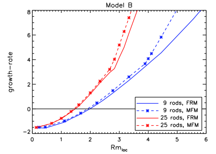
Figure 7: Growth-rate versus ${\rm{Rm}}_{\rm{loc}}$ for different configurations of model A (left panel) with $4,16,64,\mbox{ and }256$ cells and model B (right panel) with 9 and 25 rods, respectively. The solid curves denote the growth-rates from the fully resolved models (FRM) and the dashed curves denote the growth-rates for mean field models (MFM) that have been computed using the mean-field coefficients obtained for the specific ${\rm{Rm}}_{\rm{loc}}$ that are marked with the stars.

We obtain quite a good agreement between FRM and MFM if the system is not strongly overcritical. The agreement becomes better for an increasing number of helical eddies, i.e., for an increasing scale separation which provides a better fulfilment of the prerequisites for applying the mean-field theory. The rather large deviations in the strongly overcritical regime can be explained by a transition of the vertical wavenumber of the leading eigenmode from $n=1$ to $n=2$. The higher wavenumber is not incorporated by the particular vertical wave number of the applied testfields which are $\propto\cos(z)$ and $\propto\sin(z)$. In principle this issue could be attacked by computing mean-field coefficients for testfields $\propto\cos(nz)$ and $\propto\sin(nz)$ with $n=2,3,4,...$ and including these contributions in the mean field models 2008A&A…482..739Bsee, e.g.,.

The growth-rates presented in figure 7 show that a reduction of the scale of a single helical cell (or an increase of the number of helical cells) improves the dynamo properties of the system. The increase in growth-rate with decreasing $D$ follows a typical scaling law, which becomes apparent from the left panel of figure 8 where the growth-rates are plotted against ${\rm{Rm}}_{\rm{loc}}$ divided by $\sqrt{D}$. The scaling is almost perfect for small magnetic Reynolds numbers and convergence arises when changing the flow pattern from 64 to 256 cells (compare green and orange curve in the left panel in figure 8). A similar scaling is obtained for the critical magnetic Reynolds number ${\rm{Rm}_{\rm{loc}}^{\rm{crit}}}$ that is required for the onset of dynamo action.

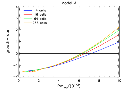
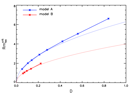
Figure 8: Left panel: growth-rate versus ${\rm{Rm}}_{\rm{loc}}$ divided by $\sqrt{D}$ for model A. Right panel: Critical value of the local magnetic Reynolds number in dependence of the cell size $D$. The dotted curves show a fit proportional to $\sqrt{D}$.

The behavior of ${\rm{Rm}_{\rm{loc}}^{\rm{crit}}}$ for decreasing cell size $D$ can be derived assuming that the onset of dynamo action is governed by some global magnetic Reynolds number. This quantity may be defined on the basis of an effective length scale that is given by the linear number of cells (which in our quadratic configuration is equal to $\sqrt{N}$) multiplied with the typical scale of a single cell $D$. Then the onset of mean-field dynamo action is determined by ${\rm{Rm}}_{\rm{glob}}^{\rm{crit}}\sim\sqrt{N}D\alpha^{\rm{crit}}/\eta$. For a large number of cells (corresponding to a small $D$) we have ${\rm{Rm}}_{\rm{loc}}\ll 1$, so that using equation (23) with $\varPhi\rightarrow 1$, we can write $\sqrt{N}D\alpha^{\rm{crit}}/\eta=\sqrt{N}K({\rm{Rm}}_{\rm{loc}}^{\rm{crit}})^{2}$. Given that we used $\sqrt{N}D=\mbox{const}$, this immediately yields ${\rm{Rm}}_{\rm{loc}}^{\rm{crit}}\sim\sqrt{D}$ which is indeed confirmed by our results (right panel in figure 8). A more detailed analysis of the critical magnetic Reynolds number for a mean field model of the Roberts flow that includes the dependence on the vertical extension can be found in tilgner02.

4.2 Walls and rods with ${\mu_{\rm{r}}>1}$

In the following, we only examine systems with $16$ eddies (model A) and $9$ rods (model B) because the consideration of a permeability distribution with $\mu_{\rm{r}}>1$ extends the necessary simulation time due to the decreased effective diffusivity, so that we are limited to smaller systems with lower grid resolution.

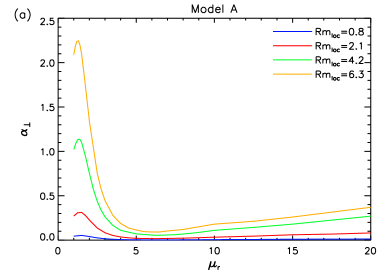
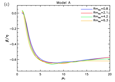
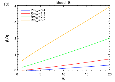
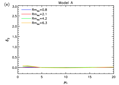
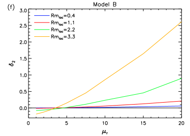
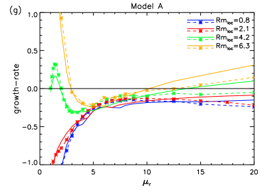
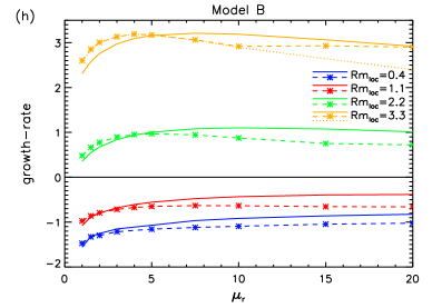
Figure 9: Mean-field coefficients and growth-rates versus $\mu_{\rm{r}}$ for various ${\rm{Rm}}_{\rm{loc}}$ (left: model A, right: model B). Top row: $\alpha_{\perp}$ versus $\mu_{\rm{r}}$, second row: $\beta$ versus $\mu_{\rm{r}}$, third row: $\delta_{2}$ versus $\mu_{\rm{r}}$, fourth row: growth-rate versus $\mu_{\rm{r}}$ and comparison between FRM (solid curves) and MFM (dashed curves and stars). The dotted orange curve in panel (h) shows the MFM growth-rates without $\delta_{2}$ term.

Not surprisingly, the results become more complex when $\mu_{\rm{r}}>1$. Figure 9a and b show the behavior of $\alpha_{\perp}$ versus $\mu_{\rm{r}}$ for different values of ${\rm{Rm}}_{\rm{loc}}$. Here we refrain from any scaling for $\alpha_{\perp}$ in order to carve out the direct influence of ${\rm{Rm}}_{\rm{loc}}$ and/or $\mu_{\rm{r}}$ on $\alpha_{\perp}$. For a fixed $\mu_{\rm{r}}$, we always find that $\alpha_{\perp}$ grows with increasing ${\rm{Rm}}_{\rm{loc}}$. However, we find significant differences between both flow models regarding the dependence on the permeability. For model A we observe a significant suppression of $\alpha_{\perp}$ for small permeabilities (say $\mu_{\rm{r}}<10$), followed by a slow recovery for further increasing $\mu_{\rm{r}}$. In contrast, for model B we see a moderate increase of $\alpha_{\perp}$ for small $\mu_{\rm{r}}$ followed by a saturation regime for $\mu_{\rm{r}}\mathrel{\mathchoice{\vbox{\offinterlineskip\halign{\hfil$\displaystyle#$\hfil\cr>\cr\sim\cr}}}{\vbox{\offinterlineskip\halign{\hfil$\textstyle#$\hfil\cr>\cr\sim\cr}}}{\vbox{\offinterlineskip\halign{\hfil$\scriptstyle#$\hfil\cr>\cr\sim\cr}}}{\vbox{\offinterlineskip\halign{\hfil$\scriptscriptstyle#$\hfil\cr>\cr\sim\cr}}}}5$ in which $\alpha_{\perp}$ becomes largely independent of $\mu_{\rm{r}}$.

For $\mu_{\rm{r}}$ only slightly above $1$ in model A, we find a sharp maximum for $\alpha_{\perp}$ around $\mu_{\rm{r}}\approx 1.5$. This maximum is retrieved again in the corresponding growth-rates (as the $\beta$-effect has no equivalent peak or drop) but the influence on the critical magnetic Reynolds numbers remains small (see below).

A significant difference between the two models is also found in the behavior of the $\beta$-effect (figure 9c and 9d). For model A, we see an abrupt transition to negative values between $\mu_{\rm{r}}=1$ and $\mu_{\rm{r}}\approx 5$, and $\beta$ remains nearly constant ($\beta\approx-0.6$) for $\mu_{\rm{r}}\mathrel{\mathchoice{\vbox{\offinterlineskip\halign{\hfil$\displaystyle#$\hfil\cr>\cr\sim\cr}}}{\vbox{\offinterlineskip\halign{\hfil$\textstyle#$\hfil\cr>\cr\sim\cr}}}{\vbox{\offinterlineskip\halign{\hfil$\scriptstyle#$\hfil\cr>\cr\sim\cr}}}{\vbox{\offinterlineskip\halign{\hfil$\scriptscriptstyle#$\hfil\cr>\cr\sim\cr}}}}5$. In model B the behavior of $\beta$ is surprisingly simple and monotonic. $\beta$ just increases linearly with increasing $\mu_{\rm{r}}$ with the slope increasing according to ${\rm{Rm}}_{\rm{loc}}$. In particular, we do not find any indications for a transition to negative values of $\beta$ with this flow configuration.

In figure 9e and f we additionally present the behavior of the coefficient $\delta_{2}$. This coefficient does not play any role for model A, but $\delta_{2}$ becomes large in model B for large ${\rm{Rm}}_{\rm{loc}}$ and $\mu_{\rm{r}}$. In this parameter regime, we see an $\alpha$-effect which is independent of $\mu_{\rm{r}}$ whereas $\beta$ is linearly increasing. This feature would be inconsistent with the growth-rates, which are also nearly independent of $\mu_{\rm{r}}$, so it requires an additional term that compensates for the losses from the $\beta$-effect. The only possibility in our models stems from the effects described by $\delta_{2}$. Indeed, this is confirmed in comparative mean-field models without the term $\propto\delta_{2}$ in which we find a decreasing growth-rate in the limit of large ${\rm{Rm}}_{\rm{loc}}$ and large $\mu_{\rm{r}}$ (see dotted orange curve in figure 9h).

Regarding the behavior of the growth-rates obtained with all relevant mean-field coefficients, we find in general a good agreement between FRM and MFM (solid and dashed curves in figure 9g and 9h). However, we see some increasing deviations at larger ${\rm{Rm}}_{\rm{loc}}$ when $\mu_{\rm{r}}\mathrel{\mathchoice{\vbox{\offinterlineskip\halign{\hfil$\displaystyle#$\hfil\cr>\cr\sim\cr}}}{\vbox{\offinterlineskip\halign{\hfil$\textstyle#$\hfil\cr>\cr\sim\cr}}}{\vbox{\offinterlineskip\halign{\hfil$\scriptstyle#$\hfil\cr>\cr\sim\cr}}}{\vbox{\offinterlineskip\halign{\hfil$\scriptscriptstyle#$\hfil\cr>\cr\sim\cr}}}}10$. In that parameter regime the growth-rates obtained from the MFM are systematically smaller than the growth-rates obtained from the FRM. The behavior of the growth-rates is not monotonic for model A, whereas for model B we find an enhancement of induction action at low $\mu_{\rm{r}}$ while the growth-rates become independent of $\mu_{\rm{r}}$ for $\mu_{\rm{r}}\mathrel{\mathchoice{\vbox{\offinterlineskip\halign{\hfil$\displaystyle#$\hfil\cr>\cr\sim\cr}}}{\vbox{\offinterlineskip\halign{\hfil$\textstyle#$\hfil\cr>\cr\sim\cr}}}{\vbox{\offinterlineskip\halign{\hfil$\scriptstyle#$\hfil\cr>\cr\sim\cr}}}{\vbox{\offinterlineskip\halign{\hfil$\scriptscriptstyle#$\hfil\cr>\cr\sim\cr}}}}10$. Considering the whole range of achievable $\mu_{\rm{r}}$ in model A we find a reduction of the critical magnetic Reynolds number from ${\rm{Rm}}^{\rm{crit}}_{\rm{loc}}\approx 4.2$ (at $\mu_{\rm{r}}=1$) to ${\rm{Rm}}^{\rm{crit}}_{\rm{loc}}\approx 3.2$ (at $\mu_{\rm{r}}=20$). However, inbetween, dynamo action is significantly suppressed by the presence of ferromagnetic walls (left hand side in figure 10) and $\rm{Rm}_{\rm{loc}}^{\rm{crit}}$ can even reach values up to $\sim 30$ around $\mu_{\rm{r}}\approx 5.5$.

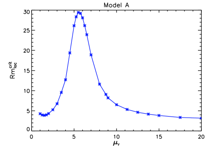
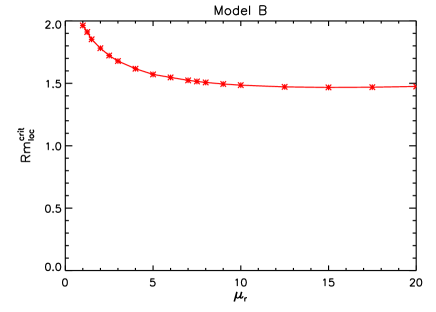
Figure 10: Critical magnetic Reynolds number for the onset of dynamo action versus permeability. Left: flow model A with 16 helical cells, right: flow model B with 9 helical cells.

For model B we see a monotonic decrease from ${\rm{Rm}}_{\rm{loc}}^{\rm{crit}}\approx 2$ at $\mu_{\rm{r}}=1$ to ${\rm{Rm}}_{\rm{loc}}^{\rm{crit}}\approx 1.5$ at $\mu_{\rm{r}}=20$. Regarding the asymptotic behavior for large $\mu_{\rm{r}}$ in figure 10 it seems unlikely that a further increase of $\mu_{\rm{r}}$ will significantly reduce the critical magnetic Reynolds number of both flow models.

5 Conclusions

We have performed numerical simulations of the kinematic induction equation for two different helical flow types including internal walls or rods that may have magnetic properties. In the limit of large permeability, we found a moderate impact of $\mu_{\rm{r}}$ on dynamo action in terms of a reduction of ${\rm{Rm}}_{\rm{loc}}^{\rm{crit}}$ of roughly 25% compared to the non-magnetic case. This relative reduction of the critical magnetic Reynolds number is nearly the same for both models. With view on the asymptotic behavior of ${\rm{Rm}}^{\rm{crit}}_{\rm{loc}}$ for large $\mu_{\rm{r}}$ we do not expect much smaller values for further increasing $\mu_{\rm{r}}$. In model A, at the fluid-wall interface (where the field is maximum) the magnetic field is predominantly parallel to the cell walls, so that the permeability is not very important. The situation is less clear for model B, for which one could guess that there is little field in the rods because of flux expulsion from the helical flow, so that the properties of the rods have little effect. Other possibilities for an explanation of the magnetic field behavior rely on the particular topology of the permeability distribution, which in our model B consists of disconnected columns. This might hamper the formation of a large scale field, however, the behavior is not unique in the whole parameter range so that more detailed investigations are required to find a convincing explanation for model B. Regarding the impact of the magnetic permeability, its influence on the critical magnetic Reynolds number is less than what could have been guessed from the results of VKS dynamo experiment. This can be explained by the dominant dynamo mode which, in the present study, can be characterized by the vertical wavenumber. Here, the leading mode has the wavenumber $k_{z}=1$, so that our results should be compared with the behavior of the simplest non-axisymmetric eigenmode in the VKS configuration (the $m=1$ mode which is $\propto\cos\varphi$). Indeed, 2012NJPh…14e3005G found a reduction of 29% from ${\rm{Rm}}^{\rm{crit}}=76$ to ${\rm{Rm}}^{\rm{crit}}=54$ for $\mu_{\rm{r}}\rightarrow\infty$ which is rather close to the reduction we obtained in our present calculations. However, both models (VKS and helical flow models in the present study) are quite different so that this accordance might be an accident. Regarding a dynamo mode with $k_{z}=0$ (which corresponds to a uniform field in the vertical direction), we do not see such a strong impact on its growth-rate as found for the axisymmetric dynamo mode in the VKS model.

Despite the similar reduction of ${\rm{Rm}}_{\rm{loc}}^{\rm{crit}}$ for both models in the limit of large $\mu_{\rm{r}}$, we find an entirely different behavior for the corresponding mean-field coefficients. For model A, the presence of magnetic walls surrounding a single helical flow cell results in a suppression of the $\alpha$-effect and a transition to a negative $\beta$-effect (which remains smaller than the “normal” diffusivity). In contrast, we see a slight enhancement of $\alpha$ and a linear growth of $\beta$ for increasing $\mu_{\rm{r}}$ in model B, where the helical flow surrounds a magnetic rod. The development of $\alpha$ and $\beta$ is not sufficient to explain the constant behavior of the growth-rates for large $\mu_{\rm{r}}$ and ${\rm{Rm}}_{\rm{loc}}$ where for increasing $\mu_{\rm{r}}$ we find a constant growth-rate, a constant $\alpha$-effect but a linearly growing (positive) $\beta$-effect. Hence, an additional dynamo supporting effect must be present in order to compensate the increasing losses due to the $\beta$-effect. The only possibility within our study is the $\delta_{2}$ effect, which indeed becomes an important contribution in that parameter regime.

Comparing the growth-rates obtained from fully resolved models with the corresponding mean-field models we found a good agreement between both approaches for non-magnetic material ($\mu_{\rm{r}}=1$) and for materials with $\mu_{\rm{r}}\mathrel{\mathchoice{\vbox{\offinterlineskip\halign{\hfil$\displaystyle#$\hfil\cr<\cr\sim\cr}}}{\vbox{\offinterlineskip\halign{\hfil$\textstyle#$\hfil\cr<\cr\sim\cr}}}{\vbox{\offinterlineskip\halign{\hfil$\scriptstyle#$\hfil\cr<\cr\sim\cr}}}{\vbox{\offinterlineskip\halign{\hfil$\scriptscriptstyle#$\hfil\cr<\cr\sim\cr}}}}20$. The main reason for discrepancies at larger $\mu_{\rm{r}}$ is the difficulty to estimate reliable values for the mean-field coefficients and the occurrence of eigenmodes with larger vertical wavenumber that are not included in our mean-field approach.

Our results can be adopted to large scale systems in which the flow consists of tens of thousands of helical flow cells that cannot be resolved in a direct numerical simulation. The simplest way does not need any information on mean-field coefficients and directly uses the scaling found for the critical magnetic Reynolds number, ${\rm{Rm}}_{\rm{loc}}^{\rm{crit}}\propto\sqrt{D}$ in the limit of small $D$ (which goes along with a large number of helical cells). However, in order to model realistic systems it is necessary to consider non-periodic (insulating) boundary conditions and the flow outside of the core which essentially describes a large recirculation cell. Such global models can hardly be modelled in direct numerical simulations of the full set of magnetohydrodynamic equations so it makes sense to model the magnetic induction due to the helical small scale flow through the corresponding mean-field effects, which in a global model only prevail in a limited region. The main contributions in such mean field models originate from the $\alpha$-effect and the $\beta$-effect. For non-magnetic internals we have confirmed that the $\alpha$-effect can be expressed in terms of a “universal” function $\Phi$ that allows a conclusion on $\alpha$ for larger systems when flow scale and flow amplitude are known. In combination with the $\beta$-effect which is roughly independent of the flow scale and behaves $\propto{\rm{Rm}}_{\rm{loc}}^{2}$ for small magnetic Reynolds numbers this allows a modelling of systems that may consist of tens of thousands of individual helical cells embedded into some large flow structure.

Of course, for any specific sodium fast reactor a reliable estimate of the dynamo effect would require further detailed knowledge, such as the size of the core, the number of fuel rods contained therein, and the total flow rate. In addition, the arrangement of the fuel rods and, thus, the flow field is not as simple as it is assumed in our idealized model. For example, the fuel rods are packed much more densely within an assembly with a hexagonal shape. A more detailed model in such a geometry would require a combination of our models A and B in order to consider the small scale helical flow within an assembly as well as the walls that separate individual assemblies. Furthermore, it should be noted that the pitch angle which describes the relation of vertical to horizontal flow may have an impact on dynamo action. In the present study, this parameter is fixed to unity assuming equipartition between horizontal and vertical flow whereas realistic fast reactors are characterized by a dominant vertical flow. Nevertheless, we believe that a consideration of these details will only result in minor modifications to our findings and are therefore of secondary importance.

References

References

- [1] \harvarditemAlemany et al.20002000JFM…403..263A Alemany A, Marty P, Plunian F \harvardand Soto J 2000 J. Fluid Mech. 403, 263–276.
- [2] \harvarditemBevir1973bevir Bevir M K 1973 J. Brit. Nucl. Eng. Soc. 12(4), 455–458.
- [3] \harvarditemBrandenburg et al.20082008A&A…482..739B Brandenburg A, Rädler K H \harvardand Schrinner M 2008 A&A 482, 739–746.
- [4] \harvarditemDobler et al.20032003PhRvE..67e6309D Dobler W, Frick P \harvardand Stepanov R 2003 Phys. Rev. E 67(5), 056309–+.
- [5] \harvarditemDubuisson et al.20122012JNuM..428….6D Dubuisson P, Carlan Y d, Garat V \harvardand Blat M 2012 J. Nucl. Mater. 428, 6–12.
- [6] \harvarditemDudley \harvardand James19891989RSPSA.425..407D Dudley M L \harvardand James R W 1989 Proc. R. Soc. London, Ser. A 425, 407–429.
- [7] \harvarditemFrick et al.20102010PhRvL.105r4502F Frick P, Noskov V, Denisov S \harvardand Stepanov R 2010 Phys. Rev. Lett. 105(18), 184502.
- [8] \harvarditemGailitis et al.20002000PhRvL..84.4365G Gailitis A, Lielausis O, Dement’ev S, Platacis E, Cifersons A, Gerbeth G, Gundrum T, Stefani F, Christen M, Hänel H \harvardand Will G 2000 Phys. Rev. Lett. 84, 4365–4368.
- [9] \harvarditemGajapathy et al.2007gajapathy Gajapathy R, Velusamy K, Selvaraj P, Chellapandi P \harvardand Chetal S 2007 Nucl. Eng. Des. 237(24), 2332–2342.
- [10] \harvarditemGiesecke et al.2010a2010GApFD.104..249G Giesecke A, Nore C, Plunian F, Laguerre R, Ribeiro A, Stefani F, Gerbeth G, Léorat J \harvardand Guermond J L 2010 Geophys. Astrophys. Fluid Dyn. 104, 249–271.
- [11] \harvarditemGiesecke et al.2010b2010PhRvL.104d4503G Giesecke A, Stefani F \harvardand Gerbeth G 2010 Phys. Rev. Lett. 104(4), 044503.
- [12] \harvarditemGiesecke et al.20122012NJPh…14e3005G Giesecke A, Nore C, Stefani F, Gerbeth G, Léorat J, Herreman W, Luddens F \harvardand Guermond J L 2012 New J. Phys. 14(5), 053005.
- [13] \harvarditemKrause \harvardand Rädler19801980mfmd.book…..K Krause F \harvardand Rädler K H 1980 Mean-field magnetohydrodynamics and dynamo theory Oxford: Pergamon Press.
- [14] \harvarditemMiralles et al.20132013PhRvE..88a3002M Miralles S, Bonnefoy N, Bourgoin M, Odier P, Pinton J F, Plihon N, Verhille G, Boisson J, Daviaud F \harvardand Dubrulle B 2013 Phys. Rev. E 88(1), 013002.
- [15] \harvarditemMonchaux et al.20072007PhRvL..98d4502M Monchaux R, Berhanu M, Bourgoin M, Moulin M, Odier P, Pinton J F, Volk R, Fauve S, Mordant N, Pétrélis F, Chiffaudel A, Daviaud F, Dubrulle B, Gasquet C, Marié L \harvardand Ravelet F 2007 Phys. Rev. Lett. 98(4), 044502.
- [16] \harvarditemNoskov et al.20122012PhRvE..85a6303N Noskov V, Denisov S, Stepanov R \harvardand Frick P 2012 Phys. Rev. E 85(1), 016303.
- [17] \harvarditemPétrélis et al.20072007GApFD.101..289P Pétrélis F, Mordant N \harvardand Fauve S 2007 Geophys. Astrophys. Fluid Dyn. 101, 289–323.
- [18] \harvarditemPierson1975pierson Pierson E J 1975 Nucl. Sci. Eng. 57(2), 155–163.
- [19] \harvarditemPlunian et al.19951995maghyd…31.4..382P Plunian F, Alemany A \harvardand Marty P 1995 Magnetohydrodynamics 31(4), 382–389.
- [20] \harvarditemPlunian et al.19991999JFM…382..137P Plunian F, Marty P \harvardand Alemany A 1999 J. Fluid Mech. 382, 137–154.
- [21] \harvarditemRädler2007mhdhistory2 Rädler K H 2007 in S Molokov, R Moreau \harvardand H. K Moffatt, eds, ‘Magnetohydrodynamics – Historical Evolution and Trends’ Springer pp. 55–72.
- [22] \harvarditemRädler \harvardand Brandenburg20032003PhRvE..67b6401R Rädler K H \harvardand Brandenburg A 2003 Phys. Rev. E 67(2), 026401.
- [23] \harvarditemRädler et al.2002a2002NPGeo…9..171R Rädler K H, Rheinhardt M, Apstein E \harvardand Fuchs H 2002a Nonlinear Processes Geophys. 9, 171–187.
- [24] \harvarditemRädler et al.2002b2002MHD….38…41R Rädler K H, Rheinhardt M, Apstein E \harvardand Fuchs H 2002b Magnetohydrodynamics 38, 41–71.
- [25] \harvarditemRoberts19701970RSPTA.266..535R Roberts G O 1970 Proc. R. Soc. London, Ser. A 266, 535–558.
- [26] \harvarditemRoberts19721972RSPTA.271..411R Roberts G O 1972 Proc. R. Soc. London, Ser. A 271, 411–454.
- [27] \harvarditemSarkar \harvardand Tilgner20052005AN….326..250S Sarkar A \harvardand Tilgner A 2005 Astron. Nachr. 326, 250–253.
- [28] \harvarditemSchrinner et al.20052005AN….326..245S Schrinner M, Rädler K H, Schmitt D, Rheinhardt M \harvardand Christensen U 2005 Astron. Nachr. 326, 245–249.
- [29] \harvarditemSchrinner et al.20072007GApFD.101…81S Schrinner M, Rädler K H, Schmitt D, Rheinhardt M \harvardand Christensen U R 2007 Geophys. Astrophys. Fluid Dyn. 101, 81–116.
- [30] \harvarditemSoto1999thesis_soto Soto J 1999 Etude cinématique de l’effet dynamo en milieu non homogène. Application aux Réacteurs à Neutrons Rapides. PhD thesis L’Institut National Polytechnique De Grenoble.
- [31] \harvarditemStefani et al.1999ISI:000080074100003 Stefani F, Gerbeth G \harvardand Gailitis A 1999 in Alemany, A and Marty, P and Thibault, JP, ed., ‘Transfer Phenomena in Magnetohydrodynamic and Electroconducting Flows’ Springer pp. 31–44.
- [32] \harvarditemStieglitz \harvardand Müller20012001PhFl…13..561S Stieglitz R \harvardand Müller U 2001 Phys. Fluids 13, 561–564.
- [33] \harvarditemTilgner2001tilgner01 Tilgner A 2004 Geophys. Astrophys. Fluid Dyn. 98(3), 225–234.
- [34] \harvarditemTilgner2007tilgner02 Tilgner A 2007 New J. Phys. 9, 290.
- [35] \harvarditemVerhille et al.20102010NJPh…12c3006V Verhille G, Plihon N, Bourgoin M, Odier P \harvardand Pinton J 2010 New J. Phys. 12(3), 033006–+.
- [36]