Empirical phi-divergence test statistics for testing simple and composite null hypotheses

Abstract

The main purpose of this paper is to introduce first a new family of empirical test statistics for testing a simple null hypothesis when the vector of parameters of interest are defined through a specific set of unbiased estimating functions. This family of test statistics is based on a distance between two probability vectors, with the first probability vector obtained by maximizing the empirical likelihood on the vector of parameters, and the second vector defined from the fixed vector of parameters under the simple null hypothesis. The distance considered for this purpose is the phi-divergence measure. The asymptotic distribution is then derived for this family of test statistics. The proposed methodology is illustrated through the well-known data of Newcomb’s measurements on the passage time for light. A simulation study is carried out to compare its performance with respect to the empirical likelihood ratio test when confidence intervals are constructed based on the respective statistics for small sample sizes. The results suggest that the “empirical modified likelihood ratio test statistic” provides a competitive alternative to the empirical likelihood ratio test statistic, and is also more robust than the empirical likelihood ratio test statistic in the presence of contamination in the data. Finally, we propose empirical phi-divergence test statistics for testing a composite null hypothesis and present some asymptotic as well as simulation results to study the performance of these test procedures.

AMS 2001 Subject Classification: 62E20

Keywords and phrases: Empirical likelihood, Empirical phi-divergence test statistics, Influence function, Phi-divergence measures, Power function, Empirical likelihood ratio, Empirical modified likelihood ratio.

1 Introduction

Empirical likelihood (EL) is a powerful and currently widely used approach for developing efficient nonparametric statistics. The EL was introduced by Owen (1988) and since then many papers have appeared on this topic making varied contributions to different inferential problems. In this approach, the parameters are usually defined as functionals of the unknown population distribution.

The first purpose of this paper is to introduce a new family of empirical test statistics as an alternative to the likelihood ratio test statistic proposed by Qin and Lawless (1994) for testing a simple null hypothesis. As an extension of the empirical likelihood ratio test of Qin and Lawless (1995), a new family of empirical test statistics is also considered here for composite hypothsis. This new family of empirical test statistics is based on divergence measures.

Consider $k$-variate i.i.d. random vectors $\mathbf{X}_{1},...,\mathbf{X}_{n}$ with unknown distribution function $F$, and a $p$-dimensional parameter, $\boldsymbol{\theta\in\Theta}$, associated with $F$ having finite mean and non-singular covariance matrix. We assume that all the information about $\boldsymbol{\theta}$ and $F$ is available in the form of $r\geq p$ functionally independent unbiased estimating functions, through the functions $g_{j}(\boldsymbol{X},\boldsymbol{\theta})$, $j=1,2,...,r$, such that $E_{F}\left[g_{j}(\boldsymbol{X},\boldsymbol{\theta})\right]=0$. In vector notation, we have $\boldsymbol{g}(\boldsymbol{X},\boldsymbol{\theta})=\left(g_{1}(\boldsymbol{X},\boldsymbol{\theta}),...,g_{r}(\boldsymbol{X},\boldsymbol{\theta}\right))^{T}$, such that

$$E_{F}\left[\boldsymbol{g}(\boldsymbol{X},\boldsymbol{\theta})\right]=\boldsymbol{0}_{r}.$$ (1)

We shall assume that for each realization $\boldsymbol{\boldsymbol{x}}$ of $\boldsymbol{\boldsymbol{X}}$, $\boldsymbol{g}:$ $\mathbb{R}^{p}\mathbb{\rightarrow R}^{r}$ is a vector-valued function and the $r\times p$ matrix

$$\boldsymbol{G}_{\boldsymbol{x}}\left(\boldsymbol{\theta}\right)=\frac{\partial\boldsymbol{g}(\boldsymbol{\boldsymbol{x}},\boldsymbol{\theta})}{\partial\boldsymbol{\theta}^{T}}$$ (2)

exists. This formulation is as in Qin and Lawless (1994), but a little different from that of Owen (1988, 1990). The essential difference is that Owen considered $r=p$ instead of $r\geq p$. For example, by taking into account that $E_{F}\left[X\right]=\theta$, we can adopt steps similar to the method of moments to obtain estimators through the estimating function $g_{1}(X,\theta)=X-\theta$ of a univariate distribution. In addition, if we assume $E_{F}\left[X^{2}\right]=2\theta^{2}+1$, the other estimating function is $g_{2}(X,\theta)=X^{2}-2\theta^{2}-1$, and in this case we have $r=2>p=k=1$.

Let $\boldsymbol{x}_{1},...,\boldsymbol{x}_{n}$ be a realization of $\boldsymbol{X}_{1},...,\boldsymbol{X}_{n}$. The empirical likelihood function is then given by

$$\mathcal{L}_{n}(F)=\prod_{i=1}^{n}dF\left(\boldsymbol{x}_{i}\right)=\prod_{i=1}^{n}p_{i},$$

where $p_{i}=dF\left(\boldsymbol{x}_{i}\right)=P(\boldsymbol{X}=\boldsymbol{x}_{i})$. Only distributions with an atom of probability at each $\boldsymbol{x}_{i}$ have non-zero likelihood, and without consideration of estimating functions, the empirical likelihood function $\mathcal{L}_{n}(F)$ is seen to be maximized, at $\boldsymbol{X}_{1}=\boldsymbol{x}_{1},...,\boldsymbol{X}_{n}=\boldsymbol{x}_{n}$, by the empirical distribution function

$$F_{n}\left(\boldsymbol{x}\right)=\sum\limits_{i=1}^{n}u_{i}I(\boldsymbol{X_{i}<x}),$$

which is associated with the $n$-dimensional discrete uniform distribution

$$\boldsymbol{u}=(u_{1},...,u_{n})^{T}=(\tfrac{1}{n},\overset{\overset{n}{\smile}}{\cdots},\tfrac{1}{n})^{T}.$$

Now, let

$$F_{n,\boldsymbol{\theta}}\left(\boldsymbol{x}\right)=\sum\limits_{i=1}^{n}p_{i}\left(\boldsymbol{\theta}\right)I(\boldsymbol{X_{i}<x})\text{,}$$

be an empirical distribution function associated with the probability vector

$$\boldsymbol{p}(\boldsymbol{\theta})=(p_{1}(\boldsymbol{\theta}),...,p_{n}(\boldsymbol{\theta}))^{T},\quad p_{i}\left(\boldsymbol{\theta}\right)\geq 0,\quad\sum\limits_{i=1}^{n}p_{i}\left(\boldsymbol{\theta}\right)=1,$$ (3)

and $\ell_{E,n}(\boldsymbol{\theta})$ be the kernel of the empirical log-likelihood function, $\sum_{i=1}^{n}\log p_{i}\left(\boldsymbol{\theta}\right)$. If we are interested in maximizing $\ell_{E,n}(\boldsymbol{\theta})$ subject to the restrictions defined by the estimating functions based on $F_{n,\boldsymbol{\theta}}\left(\boldsymbol{x}\right)$ given by

$$\sum\limits_{i=1}^{n}p_{i}\left(\boldsymbol{\theta}\right)\boldsymbol{g}(\boldsymbol{X}_{i},\boldsymbol{\theta})=\boldsymbol{0}_{r},$$ (4)

we obtain, by applying the Lagrange multipliers method,

$$p_{i}\left(\boldsymbol{\theta}\right)=\frac{1}{n}\frac{1}{1+\boldsymbol{t}(\boldsymbol{\theta})^{T}\boldsymbol{g}(\boldsymbol{X}_{i},\boldsymbol{\theta})},\text{ }i=1,...,n,$$ (5)

where $\boldsymbol{t}(\boldsymbol{\theta})$ is an $r$-dimensional vector to be determined by solving the non-linear system of $r$ equations,

$$\frac{1}{n}\sum\limits_{i=1}^{n}\frac{1}{1+\boldsymbol{t}(\boldsymbol{\theta})^{T}\boldsymbol{g}(\boldsymbol{x}_{i},\boldsymbol{\theta})}\boldsymbol{g}(\boldsymbol{X}_{i},\boldsymbol{\theta})=\boldsymbol{0}_{r},$$ (6)

subject to (3) and (5). Thus, the kernel of the empirical log-likelihood function is

$$\ell_{E,n}(\boldsymbol{\theta})=-\sum\limits_{i=1}^{n}\log\left[1+\boldsymbol{t}(\boldsymbol{\theta})^{T}\boldsymbol{g}(\boldsymbol{X}_{i},\boldsymbol{\theta})\right].$$ (7)

One of the important results of Qin and Lawless (1994) is that the empirical likelihood ratio test statistic for testing

$$H_{0}\text{: }\boldsymbol{\theta}=\boldsymbol{\theta}_{0}\text{ vs. }H_{1}\text{: }\boldsymbol{\theta\neq\theta}_{0}$$ (8)

is given by

$$L_{E,n}(\widehat{\boldsymbol{\theta}}_{E,n},\boldsymbol{\theta}_{0})=2\ell_{E,n}(\widehat{\boldsymbol{\theta}}_{E,n})-2\ell_{E,n}(\boldsymbol{\theta}_{0}),$$ (9)

where $\widehat{\boldsymbol{\theta}}_{E,n}$ is the empirical maximum likelihood estimator of the parameter $\boldsymbol{\theta}$ obtained by maximizing $\ell_{E,n}(\boldsymbol{\theta})$ in (7). In particular, if $r=p$, it can be seen that $\boldsymbol{t}(\widehat{\boldsymbol{\theta}}_{E,n})=\boldsymbol{0}_{r}$, $\boldsymbol{p}(\widehat{\boldsymbol{\theta}}_{E,n})=\boldsymbol{u}$ and $\widehat{\boldsymbol{\theta}}_{E,n}$ is the solution of the system of $r$ equations $\boldsymbol{\bar{g}}_{n}(\boldsymbol{\theta})=\boldsymbol{0}_{r}$, where

$$\boldsymbol{\bar{g}}_{n}(\boldsymbol{\theta})=\frac{1}{n}\sum\limits_{i=1}^{n}\boldsymbol{g}(\boldsymbol{X}_{i},\boldsymbol{\theta}),$$ (10)

subject to (3) and (5). Furthermore, if $r=p$, $\ell_{E,n}(\widehat{\boldsymbol{\theta}}_{E,n})=0$ and $L_{E,n}(\widehat{\boldsymbol{\theta}}_{E,n},\boldsymbol{\theta}_{0})=-2\ell_{E,n}(\boldsymbol{\theta}_{0})$. The asymptotic properties of $\widehat{\boldsymbol{\theta}}_{E,n}$, when $r\geq p$, were studied by Qin and Lawless (1994). In fact, the asymptotic distribution of $L_{E,n}(\widehat{\boldsymbol{\theta}}_{E,n},\boldsymbol{\theta}_{0})$ in (9) is chi-square with $p$ degrees of freedom.

Here, we propose a new family of test statistics for testing the hypotheses in (8), based on $\phi$-divergence measures, and then derive their asymptotic distribution. This new family of empirical test statistics is referred to hereafter as “empirical $\phi$-divergence test statistics”. In Section 3, the asymptotic null distribution of the empirical $\phi$-divergence test statistics is derived. Then, two power approximations of the empirical $\phi$-divergence test statistics are presented in Section 4. An illustrative example is presented in Section 5. In Section 6, a Monte Carlo simulation study is carried out to compare its performance with respect to the empirical likelihood ratio test when confidence intervals are constructed based on the respective statistics for small simple sizes. The results show that the empirical $\phi$-divergence test statistic is competitive in terms of power when compared to the empirical likelihood ratio test statistic, and moreover is more robust than the empirical likelihood ratio test statistic in the presence of contamination in the data. Next, in Section 7, we propose empirical phi-divergence test statistics for testing a composite null hypothesis and present some asymptotic as well as simulation results to evaluate the performance of these test procedures. Finally, in Section 8, we make some concluding remarks.

2 New family of empirical phi-divergence test statistics

The Kullback-Leibler divergence measure between the probability vectors, $\boldsymbol{u}$ and $\boldsymbol{p}(\boldsymbol{\theta})$, is given by

$$\sum\limits_{i=1}^{n}u_{i}\log\frac{u_{i}}{p_{i}(\boldsymbol{\theta})}=\sum\limits_{i=1}^{n}\frac{1}{n}\log\frac{\frac{1}{n}}{\frac{1}{n}\frac{1}{1+\boldsymbol{t}(\boldsymbol{\theta})^{T}\boldsymbol{g}(\boldsymbol{x}_{i},\boldsymbol{\theta})}}=\frac{1}{n}\sum\limits_{i=1}^{n}\log\left(1+\boldsymbol{t}(\boldsymbol{\theta})^{T}\boldsymbol{g}(\boldsymbol{x}_{i},\boldsymbol{\theta})\right).$$

In the sequel, we shall denote it by $D_{\mathrm{Kullback}}(F_{n},F_{n,\boldsymbol{\theta}})$, since the above expression is the distance, in the sense of the Kullback-Leibler divergence, between the distributions functions $F_{n}$ and $F_{n,\boldsymbol{\theta}}$. Using this notation, it is clear that the empirical likelihood ratio test statistic in (9) can be expressed as

$$L_{E,n}(\widehat{\boldsymbol{\theta}}_{E,n},\boldsymbol{\theta}_{0})=2n\left(D_{\mathrm{Kullback}}\left(F_{n},F_{n,\boldsymbol{\theta}_{0}}\right)-D_{\mathrm{Kullback}}\left(F_{n},F_{n,\widehat{\boldsymbol{\theta}}_{E,n}}\right)\right),$$

or equivalently

$$L_{E,n}\left(\widehat{\boldsymbol{\theta}}_{E,n},\boldsymbol{\theta}_{0}\right)=\frac{2n}{\phi^{\prime\prime}(1)}\left(D_{\phi}(F_{n},F_{n,\boldsymbol{\theta}_{0}})-D_{\phi}(F_{n},F_{n,\widehat{\boldsymbol{\theta}}_{E,n}})\right),$$

where

$$D_{\phi}\left(F_{n},F_{n,\boldsymbol{\theta}}\right)=\frac{1}{n}\sum\limits_{i=1}^{n}\frac{1}{1+\boldsymbol{t}(\boldsymbol{\theta})^{T}\boldsymbol{g}(\boldsymbol{x}_{i},\boldsymbol{\theta})}\phi\left(1+\boldsymbol{t}(\boldsymbol{\theta})^{T}\boldsymbol{g}(\boldsymbol{x}_{i},\boldsymbol{\theta})\right),$$ (11)

with $\phi\left(x\right)=x\log x-x+1$, $x\in\mathbb{R}$.

Now, we shall denote by $\Phi^{\ast}$ the class of all convex functions $\phi:\mathbb{R}^{+}\longrightarrow\mathbb{R}$ such that at $x=1$, $\phi\left(1\right)=0$, $\phi^{\prime\prime}\left(1\right)>0$, and at $x=0$, $0\phi\left(0/0\right)=0$ and $0\phi\left(p/0\right)=p\lim_{u\rightarrow\infty}\frac{\phi\left(u\right)}{u}$. Instead of $\phi\left(x\right)=x\log x-x+1$, if we consider a function $\phi$ belonging to $\Phi^{\ast}$, we obtain a new family of test statistics for testing (8) given by

$$T_{n}^{\phi}(\widehat{\boldsymbol{\theta}}_{E,n},\boldsymbol{\theta}_{0})=\frac{2n}{\phi^{\prime\prime}(1)}\left(D_{\phi}(F_{n},F_{n,\boldsymbol{\theta}_{0}})-D_{\phi}(F_{n},F_{n,\widehat{\boldsymbol{\theta}}_{E,n}})\right).$$ (12)

We will refer to this family of test statistics as empirical $\phi$-divergence test statistics.

For every $\phi\in\Phi^{\ast}$ that is differentiable at $x=1$, the function $\psi\left(x\right)\equiv\phi(x)-\phi^{\prime}\left(1\right)\left(x-1\right)$ also belongs to $\Phi^{\ast}$. Then, we have

$$T_{n}^{\phi}(\widehat{\boldsymbol{\theta}}_{E,n},\boldsymbol{\theta}_{0})=T_{n}^{\psi}(\widehat{\boldsymbol{\theta}}_{E,n},\boldsymbol{\theta}_{0})$$

and $\psi$ has the additional property that $\psi^{\prime}\left(1\right)=0.$ Since the two divergence measures are equivalent, we can consider the set $\Phi^{\ast}$ to be equivalent to the set $\Phi=\Phi^{\ast}\cap\left\{\phi:\phi^{\prime}\left(1\right)=0\right\}$. In what follows, we shall assume that $\phi\in\Phi$.

The statistics in (12) have been considered recently by Broniatowski and Keziou (2012) to give some empirical test statistics, generalizing an important subfamily of test statistics introduced by Baggerly (1998). We present more details in Section 6 in this regard.

The main purpose of this paper is to present a new family of test statistics for testing the hypotheses in (8) based on the $\phi$-divergence measure between $F_{n,\boldsymbol{\theta}_{0}}$ and $F_{n,\widehat{\boldsymbol{\theta}}_{E,n}}$, namely, $D_{\phi}\left(F_{n,\widehat{\boldsymbol{\theta}}_{E,n}},F_{n,\boldsymbol{\theta}_{0}}\right)$. We shall consider the empirical family of $\phi$-divergence test statistics given by

$$S_{n}^{\phi}(\widehat{\boldsymbol{\theta}}_{E,n},\boldsymbol{\theta}_{0})=\frac{2n}{\phi^{\prime\prime}(1)}D_{\phi}\left(F_{n,\widehat{\boldsymbol{\theta}}_{E,n}},F_{n,\boldsymbol{\theta}_{0}}\right)=\frac{2}{\phi^{\prime\prime}(1)}\sum\limits_{i=1}^{n}\frac{1}{1+\boldsymbol{t}(\boldsymbol{\theta}_{0})^{T}\boldsymbol{g}(\boldsymbol{x}_{i},\boldsymbol{\theta}_{0})}\phi\left(\frac{1+\boldsymbol{t}(\boldsymbol{\theta}_{0})^{T}\boldsymbol{g}(\boldsymbol{x}_{i},\boldsymbol{\theta}_{0})}{1+\boldsymbol{t}(\widehat{\boldsymbol{\theta}}_{E,n})^{T}\boldsymbol{g}(\boldsymbol{x}_{i},\widehat{\boldsymbol{\theta}}_{E,n})}\right),$$ (13)

where $\phi$ is a function satisfying the same conditions as function $\phi$ used to construct $T_{n}^{\phi}(\widehat{\boldsymbol{\theta}}_{E,n},\boldsymbol{\theta}_{0})$. Observe that (12) and (13) are equivalent only when $r=p$. It is well-known that the family of test statistics based on $\phi$-divergence has some nice and optimal properties for different inferential problems, and especially in relation to robustness; see Pardo (2006) and Basu et al. (2011).

3 Asymptotic null distribution

In this section, we derive the asymptotic distribution of $S_{n}^{\phi}(\widehat{\boldsymbol{\theta}}_{E,n},\boldsymbol{\theta}_{0})$. For this purpose, the asymptotic distribution of the maximum empirical likelihood estimator of the parameter $\boldsymbol{\theta}$, $\widehat{\boldsymbol{\theta}}_{E,n},$ as well as the asymptotic distribution of $\widehat{\boldsymbol{t}}=\boldsymbol{t}(\widehat{\boldsymbol{\theta}}_{E,n})$ are important. These asymptotic distributions are given in Qin and Lawless (1994), for example. Under some regularity assumptions (see Lemma 1 and Theorem 1 of Qin and Lawless (1994)), we have

$$\sqrt{n}\begin{pmatrix}\widehat{\boldsymbol{\theta}}_{E,n}-\boldsymbol{\theta}_{0}\\ \boldsymbol{t}(\widehat{\boldsymbol{\theta}}_{E,n})\end{pmatrix}\overset{\mathcal{L}}{\underset{n\rightarrow\infty}{\longrightarrow}}\mathcal{N}\left(\boldsymbol{0}_{p+r},\begin{pmatrix}\boldsymbol{V}\left(\boldsymbol{\theta}_{0}\right)&\boldsymbol{0}_{p\times r}\\ \boldsymbol{0}_{r\times p}&\boldsymbol{R}\left(\boldsymbol{\theta}_{0}\right)\end{pmatrix}\right),$$ (14)

where $\overset{\mathcal{L}}{\underset{n\rightarrow\infty}{\longrightarrow}}$ denotes convergence in law and

$$\boldsymbol{V}\left(\boldsymbol{\theta}_{0}\right) =\left(\boldsymbol{S}_{12}\left(\boldsymbol{\theta}_{0}\right)^{T}\boldsymbol{S}_{11}^{-1}\left(\boldsymbol{\theta}_{0}\right)\boldsymbol{S}_{12}\left(\boldsymbol{\theta}_{0}\right)\right)^{-1},$$ (15)

$$\boldsymbol{R}\left(\boldsymbol{\theta}_{0}\right) =\boldsymbol{S}_{11}^{-1}\left(\boldsymbol{\theta}_{0}\right)-\boldsymbol{S}_{11}^{-1}\left(\boldsymbol{\theta}_{0}\right)\boldsymbol{S}_{12}\left(\boldsymbol{\theta}_{0}\right)\boldsymbol{V}\left(\boldsymbol{\theta}_{0}\right)\boldsymbol{S}_{21}\left(\boldsymbol{\theta}_{0}\right)\boldsymbol{S}_{11}^{-1}\left(\boldsymbol{\theta}_{0}\right),$$ (16)

with

$$\boldsymbol{S}_{11}\left(\boldsymbol{\theta}_{0}\right) =E_{F}\left[\boldsymbol{g}\left(\boldsymbol{X},\boldsymbol{\theta}_{0}\right)\boldsymbol{g}\left(\boldsymbol{X},\boldsymbol{\theta}_{0}\right)^{T}\right],$$ (17)

$$\boldsymbol{S}_{12}\left(\boldsymbol{\theta}_{0}\right) =E_{F}\left[\boldsymbol{G}_{\boldsymbol{X}}(\boldsymbol{\theta}_{0})\right],\quad\boldsymbol{S}_{21}\left(\boldsymbol{\theta}_{0}\right)=\boldsymbol{S}_{12}\left(\boldsymbol{\theta}_{0}\right)^{T}.$$ (18)

This result is derived from:
a)

$$\sqrt{n}(\widehat{\boldsymbol{\theta}}_{E,n}-\boldsymbol{\theta}_{0})=\boldsymbol{V\left(\boldsymbol{\theta}_{0}\right)S}_{12}\left(\boldsymbol{\theta}_{0}\right)^{T}\boldsymbol{S}_{11}^{-1}\left(\boldsymbol{\theta}_{0}\right)\sqrt{n}\boldsymbol{\bar{g}}_{n}(\boldsymbol{\theta}_{0})+o_{p}(\boldsymbol{1}_{p}),$$ (19)

where $\boldsymbol{\bar{g}}_{n}\left(\boldsymbol{\theta}\right)$ is given by (10). It is clear from the Central Limit Theorem that

$$\sqrt{n}\boldsymbol{\bar{g}}_{n}(\boldsymbol{\theta}_{0})\overset{\mathcal{L}}{\underset{n\rightarrow\infty}{\longrightarrow}}\mathcal{N}(\boldsymbol{0}_{r},\boldsymbol{S}_{11}\left(\boldsymbol{\theta}_{0}\right)),$$

and so $\sqrt{n}(\widehat{\boldsymbol{\theta}}_{E,n}-\boldsymbol{\theta}_{0})\overset{\mathcal{L}}{\underset{n\rightarrow\infty}{\longrightarrow}}\mathcal{N}(\boldsymbol{0}_{p},\boldsymbol{V}\left(\boldsymbol{\theta}_{0}\right))$;
b) $\sqrt{n}\boldsymbol{t}(\widehat{\boldsymbol{\theta}}_{E,n})=-\boldsymbol{R}\left(\boldsymbol{\theta}_{0}\right)\sqrt{n}\boldsymbol{\bar{g}}_{n}(\boldsymbol{\theta}_{0})+o_{p}(\boldsymbol{1}_{r})$, where $\boldsymbol{R}\left(\boldsymbol{\theta}_{0}\right)$ is given by (16) and so $\sqrt{n}\boldsymbol{t}(\widehat{\boldsymbol{\theta}}_{E,n})\overset{\mathcal{L}}{\underset{n\rightarrow\infty}{\longrightarrow}}\mathcal{N}(\boldsymbol{0}_{r},\boldsymbol{R}\left(\boldsymbol{\theta}_{0}\right))$.
In addition, $\widehat{\boldsymbol{\theta}}_{E,n}$ and $\boldsymbol{t}(\widehat{\boldsymbol{\theta}}_{E,n})$ are asymptotically uncorrelated.

Lemma 1

The influence function of the empirical maximum likelihood estimator of parameter $\boldsymbol{\theta}$, $\widehat{\boldsymbol{\theta}}_{E,n}$, is given by

$$\mathcal{IF}(\boldsymbol{x},\widehat{\boldsymbol{\theta}}_{E,n},F_{n,\boldsymbol{\theta}_{0}})=\boldsymbol{V\left(\boldsymbol{\theta}_{0}\right)S}_{12}\left(\boldsymbol{\theta}_{0}\right)^{T}\boldsymbol{S}_{11}^{-1}\left(\boldsymbol{\theta}_{0}\right)\boldsymbol{g}(\boldsymbol{x},\boldsymbol{\theta}_{0}).$$ (20)

Proof. It follows from the expression given in (19) and taking into account the definition of the influence function given in formula (20.1) of van der Vaart (2000, page 292).   

Remark 2

The empirical maximum likelihood estimator of parameter $\boldsymbol{\theta}$, $\widehat{\boldsymbol{\theta}}_{E,n}$, is obtained maximizing the kernel of empirical log-likelihood function given in (7) or equivalently minimizing the function $-\frac{1}{n}{\textstyle\sum\nolimits_{i=1}^{n}}\log\left(np_{i}\left(\boldsymbol{\theta}\right)\right)$, subject to the restrictions given in (4). This expression can be written as the $\phi$-divergence measure between the probability vectors $\boldsymbol{u}$ and $\boldsymbol{p}\left(\boldsymbol{\theta}\right)$, i.e. $D_{\phi}\left(F_{n},F_{n,\boldsymbol{\theta}}\right)={\textstyle\sum\nolimits_{i=1}^{n}}p_{i}\left(\boldsymbol{\theta}\right)\phi\left(\frac{1}{np_{i}\left(\boldsymbol{\theta}\right)}\right)$ with $\phi\left(x\right)=x\log x-x+1$. Therefore,

$$\widehat{\boldsymbol{\theta}}_{E,n}=\arg\min_{\theta}D_{\phi}\left(F_{n},F_{n,\boldsymbol{\theta}}\right),\text{\quad}\phi(x)=x\log x-x+1,$$

subject to the restrictions given in (4). If we consider a general function $\phi\in\Phi$, defined in Section 2, instead of considering $\phi\left(x\right)=x\log x-x+1$, then we can define the empirical minimum $\phi$-divergence estimator by

$$\widehat{\boldsymbol{\theta}}_{E\phi,n}=\arg\min_{\boldsymbol{\theta}}D_{\phi}\left(F_{n},F_{n,\boldsymbol{\theta}}\right),\text{\quad}\phi\in\Phi,$$

subject to the restrictions given in (4). The empirical exponential tilting estimator (ET), considered for instance in Schennach (2007), is defined by $\widehat{\boldsymbol{\theta}}_{ET,n}=\arg\min_{\boldsymbol{\theta}}{\textstyle\sum\nolimits_{i=1}^{n}}p_{i}\left(\boldsymbol{\theta}\right)\log\left(np_{i}\left(\boldsymbol{\theta}\right)\right)$, subject to the restrictions given in (4). The ET is another member of this family of estimators since $\widehat{\boldsymbol{\theta}}_{ET,n}=\widehat{\boldsymbol{\theta}}_{E\phi,n}$ with $\phi(x)=-\log x+x-1$. The asymptotic properties of $\widehat{\boldsymbol{\theta}}_{E\phi,n}$ and $\widehat{\boldsymbol{\theta}}_{E,n}$ are the same (for more details, see Ragusa (2011), Broniatowski and Keziou (2012) and Schennach (2007)). The Fisher consistence of $\widehat{\boldsymbol{\theta}}_{E\phi,n}$ was established in Ragusa (2011). Therefore, all the asymptotic results obtained for the test statistics considered in this paper are valid replacing $\widehat{\boldsymbol{\theta}}_{E,n}$ by $\widehat{\boldsymbol{\theta}}_{E\phi,n}$. The expression given in (20), for the influence function of the empirical maximum likelihood estimator of parameter $\boldsymbol{\theta}$, can be found for the empirical minimum $\phi$-divergence estimators, $\widehat{\boldsymbol{\theta}}_{E\phi,n}$, in Proposition 2.3 of Toma (2013). Hence, all the estimators based on $\phi$-divergence measures, independently of the $\phi$ function, share the same influence function.

Let $\left\|\cdot\right\|$ denote any vector or matrix norm. We shall assume the following regularity conditions:

1. $\boldsymbol{S}_{11}\left(\boldsymbol{\theta}_{0}\right)$ in (17) is positive definite, and for $\boldsymbol{S}_{12}\left(\boldsymbol{\theta}_{0}\right)$ in (18), $\mathrm{rank}(\boldsymbol{S}_{12}\left(\boldsymbol{\theta}_{0}\right))=p$.

2. There exists a neighbourhood of $\boldsymbol{\theta}_{0}$, in which $\left\|\boldsymbol{g}\left(\boldsymbol{x},\boldsymbol{\theta}\right)\right\|^{3}$ is bounded by some integrable function.

3. There exists a neighbourhood of $\boldsymbol{\theta}_{0}$, in which $\boldsymbol{G}_{\boldsymbol{x}}(\boldsymbol{\theta})$, given in (2), is continuous and $\left\|\boldsymbol{G}_{\boldsymbol{x}}(\boldsymbol{\theta})\right\|$ is bounded by some integrable function.

4. There exists a neighbourhood of $\boldsymbol{\theta}_{0}$ in which $\frac{\partial\boldsymbol{G}_{\boldsymbol{x}}(\boldsymbol{\theta})}{\partial\boldsymbol{\theta}}$ is continuous and $\left\|\frac{\partial\boldsymbol{G}_{\boldsymbol{x}}(\boldsymbol{\theta})}{\partial\boldsymbol{\theta}}\right\|$ is bounded by some integrable function.

The asymptotic distribution of the empirical $\phi$-divergence test statistics, $S_{n}^{\phi}(\widehat{\boldsymbol{\theta}}_{E,n},\boldsymbol{\theta}_{0})$, is given in the following theorem.

Theorem 3

Under $H_{0}$ in (8) and the assumptions i)-iv) above, we have

$$S_{n}^{\phi}(\widehat{\boldsymbol{\theta}}_{E,n},\boldsymbol{\theta}_{0})\overset{\mathcal{L}}{\underset{n\rightarrow\infty}{\longrightarrow}}\chi_{p}^{2}.$$

Proof. Based on the Taylor expansions of (13), as well as the asymptotic properties of $\widehat{\boldsymbol{\theta}}_{E,n}$, given in Qin and Lawless (1994), it holds

$$S_{n}^{\phi}(\widehat{\boldsymbol{\theta}}_{E,n},\boldsymbol{\theta}_{0})=\boldsymbol{U}_{n}(\widehat{\boldsymbol{\theta}}_{E,n},\boldsymbol{\theta}_{0})^{T}\boldsymbol{U}_{n}(\widehat{\boldsymbol{\theta}}_{E,n},\boldsymbol{\theta}_{0})+o_{p}(1),$$ (21)

with $\boldsymbol{U}_{n}(\widehat{\boldsymbol{\theta}}_{E,n},\boldsymbol{\theta}_{0})=\sqrt{n}\boldsymbol{V}^{-1/2}\left(\boldsymbol{\theta}_{0}\right)(\widehat{\boldsymbol{\theta}}_{E,n}-\boldsymbol{\theta}_{0})\overset{\mathcal{L}}{\underset{n\rightarrow\infty}{\longrightarrow}}\mathcal{N}(\boldsymbol{0}_{p},\boldsymbol{I}_{p})$, according to (14).   

Remark 4

There are some measures of divergence which can not be expressed as a $\phi$-divergence measure such as the divergence measures of Bhattacharya (1943), Rényi (1961), and Sharma and Mittal (1977). However, such measures can be written in the form

$$D_{\phi}^{h}\left(F_{n,\theta},F_{n,\boldsymbol{\theta}_{0}}\right)=h\left(D_{\phi}\left(F_{n,\theta},F_{n,\boldsymbol{\theta}_{0}}\right)\right),$$

where $h$ is a differentiable increasing function mapping from $\left[0,\infty\right)$ onto $\left[0,\infty\right)$, with $h(0)=0$, $h^{\prime}(0)>0$, and $\phi\in\Phi$. In Table 1, these divergence measures are presented, along with the corresponding expressions of $h$ and $\phi$.

Divergence $h\left(x\right)$ $\phi\left(x\right)$ Rényi $\frac{1}{a\left(a-1\right)}\log\left(a\left(a-1\right)x+1\right),\quad a\neq 0,1$ $\frac{x^{a}-a\left(x-1\right)-1}{a\left(a-1\right)},\quad a\neq 0,1$ Sharma-Mittal $\frac{1}{b-1}\left\{[1+a\left(a-1\right)x]^{\frac{b-1}{a-1}}-1\right\},\quad b,a\neq 1$ $\frac{x^{a}-a\left(x-1\right)-1}{a\left(a-1\right)},\quad a\neq 0,1$ Battacharya $-\log\left(-x+1\right)$ $-x^{1/2}+\frac{1}{2}\left(x+1\right)$

Table 1: Some specific $(h,\phi)$-divergence measures.

In the case of Rényi’s divergence, we have

$$D_{\text{{R\'{e}nyi}}}^{a}\left(F_{n,\theta},F_{n,\boldsymbol{\theta}_{0}}\right)=\frac{1}{a\left(a-1\right)}\log\sum\limits_{i=1}^{n}\frac{\left(1+\boldsymbol{t}(\boldsymbol{\theta}_{0})^{T}\boldsymbol{g}(\boldsymbol{x}_{i},\boldsymbol{\theta}_{0})\right)^{a-1}}{n\left(1+\boldsymbol{t}(\boldsymbol{\theta})^{T}\boldsymbol{g}(\boldsymbol{x}_{i},\boldsymbol{\theta})\right)^{a}}\text{, if }a\neq 0,1,$$ (22)

and its “limit” cases corresponding to $a=0$ and $a=1$ as

$$D_{\text{{R\'{e}nyi}}}^{0}\left(F_{n,\theta},F_{n,\boldsymbol{\theta}_{0}}\right) =\lim_{a\rightarrow 0}D_{\text{{R\'{e}nyi}}}\left(F_{n,\theta},F_{n,\boldsymbol{\theta}_{0}}\right)=D_{\mathrm{Kullback}}\left(F_{n,\boldsymbol{\theta}_{0}},F_{n,\theta}\right)$$

$$=\sum\limits_{i=1}^{n}\frac{1}{n(1+\boldsymbol{t}(\boldsymbol{\theta})^{T}\boldsymbol{g}(\boldsymbol{x}_{i},\boldsymbol{\theta}))}\log\left(\frac{1+\boldsymbol{t}(\boldsymbol{\theta}_{0})^{T}\boldsymbol{g}(\boldsymbol{x}_{i},\boldsymbol{\theta}_{0})}{1+\boldsymbol{t}(\boldsymbol{\theta})^{T}\boldsymbol{g}(\boldsymbol{x}_{i},\boldsymbol{\theta})}\right)$$

and

$$D_{\text{{R\'{e}nyi}}}^{1}\left(F_{n,\theta},F_{n,\boldsymbol{\theta}_{0}}\right) =\lim_{a\rightarrow 1}D_{\text{{R\'{e}nyi}}}\left(F_{n,\theta},F_{n,\boldsymbol{\theta}_{0}}\right)=D_{\mathrm{Kullback}}\left(F_{n,\theta},F_{n,\boldsymbol{\theta}_{0}}\right)$$

$$=\sum\limits_{i=1}^{n}\frac{1}{n(1+\boldsymbol{t}(\boldsymbol{\theta}_{0})^{T}\boldsymbol{g}(\boldsymbol{x}_{i},\boldsymbol{\theta}_{0}))}\log\left(\frac{1+\boldsymbol{t}(\boldsymbol{\theta})^{T}\boldsymbol{g}(\boldsymbol{x}_{i},\boldsymbol{\theta})}{1+\boldsymbol{t}(\boldsymbol{\theta}_{0})^{T}\boldsymbol{g}(\boldsymbol{x}_{i},\boldsymbol{\theta}_{0})}\right),$$

respectively.

The $(h,\phi)$-divergence measures were introduced in Menéndez et al. (1995) and some associated asymptotic results were established in Menéndez et al. (1997).

Theorem 5

Under the assumptions of Theorem 3, the asymptotic null distribution of the family of empirical test statistics

$$S_{n}^{\phi,h}(\widehat{\boldsymbol{\theta}}_{E,n},\boldsymbol{\theta}_{0})=\frac{2n}{\phi^{\prime\prime}(1)h^{\prime}(0)}h\left(D_{\phi}(F_{n,\widehat{\boldsymbol{\theta}}_{E,n}},F_{n,\boldsymbol{\theta}_{0}})\right)$$

is chi-squared with $p$ degrees of freedom.

Remark 6

Note that we can also consider the family of empirical $(h,\phi)$-divergence test statistics given by

$$T_{n}^{\phi,h}(\widehat{\boldsymbol{\theta}}_{E,n},\boldsymbol{\theta}_{0})=\frac{2n}{\phi^{\prime\prime}(1)h^{\prime}(0)}\left(h\left(D_{\phi}(F_{n},F_{n,\boldsymbol{\theta}_{0}})\right)-h\left(D_{\phi}(F_{n},F_{{}_{\widehat{\boldsymbol{\theta}}_{E,n}}})\right)\right),$$

and their asymptotic distribution is chi-squared with $p$ degrees of freedom as well. Test-statistics $T_{n}^{\phi,h}(\widehat{\boldsymbol{\theta}}_{E,n},\boldsymbol{\theta}_{0})$ and $S_{n}^{\phi,h}(\widehat{\boldsymbol{\theta}}_{E,n},\boldsymbol{\theta}_{0})$, include as particular cases $T_{n}^{\phi}(\widehat{\boldsymbol{\theta}}_{E,n},\boldsymbol{\theta}_{0})$ and $S_{n}^{\phi}(\widehat{\boldsymbol{\theta}}_{E,n},\boldsymbol{\theta}_{0})$, taking $h(x)=x$. In the same way done for $S_{n}^{\phi}(\widehat{\boldsymbol{\theta}}_{E,n},\boldsymbol{\theta}_{0})$ in (21), it may be concluded that all of them have a Taylor expansion of second order which does not depend on $\phi$ or $h$,

$$T_{n}^{\phi,h}(\widehat{\boldsymbol{\theta}}_{E,n},\boldsymbol{\theta}_{0})=\boldsymbol{U}_{n}(\widehat{\boldsymbol{\theta}}_{E,n},\boldsymbol{\theta}_{0})^{T}\boldsymbol{U}_{n}(\widehat{\boldsymbol{\theta}}_{E,n},\boldsymbol{\theta}_{0})+o_{p}(1),\quad\text{and}\quad S_{n}^{\phi,h}(\widehat{\boldsymbol{\theta}}_{E,n},\boldsymbol{\theta}_{0})=\boldsymbol{U}_{n}(\widehat{\boldsymbol{\theta}}_{E,n},\boldsymbol{\theta}_{0})^{T}\boldsymbol{U}_{n}(\widehat{\boldsymbol{\theta}}_{E,n},\boldsymbol{\theta}_{0})+o_{p}(1),$$

with $\boldsymbol{U}_{n}(\widehat{\boldsymbol{\theta}}_{E,n},\boldsymbol{\theta}_{0})=\sqrt{n}\boldsymbol{V}^{-1/2}\left(\boldsymbol{\theta}_{0}\right)(\widehat{\boldsymbol{\theta}}_{E,n}-\boldsymbol{\theta}_{0})\overset{\mathcal{L}}{\underset{n\rightarrow\infty}{\longrightarrow}}\mathcal{N}(\boldsymbol{0}_{r},\boldsymbol{I}_{p})$. With regard to their influence function, a second order influence function have to be considered since the first order one vanishes (see van der Vaart (2000, Section 20.1.1)), and its expression is given by

$$\mathcal{IF}_{2}\left(\boldsymbol{x},T_{n}^{\phi,h}(\widehat{\boldsymbol{\theta}}_{E,n},\boldsymbol{\theta}_{0}),F_{n,\boldsymbol{\theta}_{0}}\right)=\mathcal{IF}_{2}\left(\boldsymbol{x},S_{n}^{\phi,h}(\widehat{\boldsymbol{\theta}}_{E,n},\boldsymbol{\theta}_{0}),F_{n,\boldsymbol{\theta}_{0}}\right)=\mathcal{IF}_{2}\left(\boldsymbol{x},\left\|\boldsymbol{U}_{n}(\widehat{\boldsymbol{\theta}}_{E,n},\boldsymbol{\theta}_{0})\right\|^{2},F_{n,\boldsymbol{\theta}_{0}}\right)$$ (23)

$$=2\left\|\boldsymbol{V}^{-1/2}\left(\boldsymbol{\theta}_{0}\right)\mathcal{IF}(\boldsymbol{x},\widehat{\boldsymbol{\theta}}_{E,n},F_{n,\boldsymbol{\theta}_{0}})\right\|^{2}=2\boldsymbol{g}(\boldsymbol{x},\boldsymbol{\theta}_{0})^{T}\boldsymbol{S}_{11}^{-1}\left(\boldsymbol{\theta}_{0}\right)\boldsymbol{S}_{12}\left(\boldsymbol{\theta}_{0}\right)\boldsymbol{V\left(\boldsymbol{\theta}_{0}\right)S}_{12}\left(\boldsymbol{\theta}_{0}\right)^{T}\boldsymbol{S}_{11}^{-1}\left(\boldsymbol{\theta}_{0}\right)\boldsymbol{g}(\boldsymbol{x},\boldsymbol{\theta}_{0}).$$

The first and second equality come from the previous second order Taylor expansion, the third one from Heritier and Ronchetti (1994) and the last one from Lemma 1. It suggests that under the simple null hypothesis, all members of both family of test-statistics have the same infinitesimal robustness. This is not a strange result, since in Lemma 1 of Toma (2009) a similar conclusion has been reached based on power divergence measures for parametric models.

4 Two approximations of power

Based on the null distribution presented in Theorem 3, we reject the null hypothesis in (8) in favour of the alternative hypothesis, if $S_{n}^{\phi}(\widehat{\boldsymbol{\theta}}_{E,n},\boldsymbol{\theta}_{0})>\chi_{p,\alpha}^{2}$, where $\chi_{p,\alpha}^{2}$ is the $\left(1-\alpha\right)$-th quantile of the chi-squared distribution with $p$ degrees of freedom.

In most cases, the power function of this test procedure can not be derived explicitly. In the following theorem, we present an asymptotic result, which provides an approximation of the power of the test.

Theorem 7

Let $\boldsymbol{\theta}^{\ast}$ be the true parameter value with $\boldsymbol{\theta}^{\ast}\neq\boldsymbol{\theta}_{0}$. Under the assumptions of Theorem 3 and $E_{F}\left[\sup_{\boldsymbol{\theta\in\Theta}}\left\|\boldsymbol{g}\left(\boldsymbol{X},\boldsymbol{\theta}\right)\right\|^{2}\right]<\infty$, we have

$$\sqrt{n}\left(D_{\phi}(F_{n,\widehat{\boldsymbol{\theta}}_{E,n}},F_{n,\boldsymbol{\theta}_{0}})-D_{\phi}(F_{n,\boldsymbol{\theta}^{\ast}},F_{n,\boldsymbol{\theta}_{0}})\right)\overset{\mathcal{L}}{\underset{n\rightarrow\infty}{\longrightarrow}}\mathcal{N}\left(0,\sigma_{\phi}^{2}\left(\boldsymbol{\theta}^{\ast},\boldsymbol{\boldsymbol{\theta}_{0}}\right)\right),$$

where

$$\sigma_{\phi}^{2}\left(\boldsymbol{\theta}^{\ast},\boldsymbol{\boldsymbol{\theta}_{0}}\right)=\boldsymbol{\tau}_{\phi}\left(\boldsymbol{\theta}^{\ast},\boldsymbol{\boldsymbol{\theta}_{0}}\right)^{T}\boldsymbol{V\left(\boldsymbol{\theta}_{0}\right)\tau}_{\phi}\left(\boldsymbol{\theta}^{\ast},\boldsymbol{\boldsymbol{\theta}_{0}}\right)$$

with

$$\boldsymbol{\tau}_{\phi}(\boldsymbol{\theta}^{\ast},\boldsymbol{\boldsymbol{\theta}_{0}})=\left(\tau_{1}^{\phi}\left(\boldsymbol{\theta}^{\ast},\boldsymbol{\boldsymbol{\theta}_{0}}\right),...,\tau_{p}^{\phi}\left(\boldsymbol{\theta}^{\ast},\boldsymbol{\boldsymbol{\theta}_{0}}\right)\right)^{T}=\left.\frac{\partial}{\partial\boldsymbol{\theta}}D_{\phi}(F_{n,\boldsymbol{\theta}},F_{n,\boldsymbol{\theta}_{0}})\right|_{\boldsymbol{\theta}=\boldsymbol{\theta}^{\ast}},$$ (24)

and the matrix $\boldsymbol{V\left(\boldsymbol{\theta}_{0}\right)}$ as defined in (15).

Proof. A first-order Taylor expansion gives

$$D_{\phi}(F_{n,\widehat{\boldsymbol{\theta}}_{E,n}},F_{n,\boldsymbol{\theta}_{0}})=D_{\phi}(F_{n,\boldsymbol{\theta}^{\ast}},F_{n,\boldsymbol{\theta}_{0}})+\boldsymbol{\tau}_{\phi}\left(\boldsymbol{\theta}^{\ast},\boldsymbol{\boldsymbol{\theta}_{0}}\right)^{T}(\widehat{\boldsymbol{\theta}}_{E,n}-\boldsymbol{\theta}^{\ast})+o(||\widehat{\boldsymbol{\theta}}_{E,n}-\boldsymbol{\theta}^{\ast}||).$$

But,

$$\sqrt{n}(\widehat{\boldsymbol{\theta}}_{E,n}-\boldsymbol{\theta}^{\ast})\overset{\mathcal{L}}{\underset{n\rightarrow\infty}{\longrightarrow}}\mathcal{N}(\boldsymbol{0}_{p},\boldsymbol{V}(\boldsymbol{\boldsymbol{\theta}_{0}})),$$

and so $\sqrt{n}\,o(||\widehat{\boldsymbol{\theta}}_{E,n}-\boldsymbol{\theta}^{\ast}||)=o_{p}(\boldsymbol{1}_{r})$. Thus, the random variables

$$\sqrt{n}\left(D_{\phi}(F_{n,\widehat{\boldsymbol{\theta}}_{E,n}},F_{n,\boldsymbol{\theta}_{0}})-D_{\phi}(F_{n,\boldsymbol{\theta}^{\ast}},F_{n,\boldsymbol{\theta}_{0}})\right)\text{ and }\boldsymbol{\tau}_{\phi}(\boldsymbol{\theta}^{\ast},\boldsymbol{\boldsymbol{\theta}_{0}})\sqrt{n}(\widehat{\boldsymbol{\theta}}_{E,n}-\boldsymbol{\theta}^{\ast})$$

have the same asymptotic distribution, and hence the desired result.   

Remark 8

It is straightforward to extend Theorem 7 for $(h,\phi)$-divergence measures $D_{\phi}^{h}\left(F_{n,\theta},F_{n,\boldsymbol{\theta}_{0}}\right)=$$h\left(D_{\phi}\left(F_{n,\theta},F_{n,\boldsymbol{\theta}_{0}}\right)\right)$, as follows. Since $h(x)-h(x_{0})=h^{\prime}(x_{0})(x-x_{0})+o(x-x_{0})$, we have

$$\sqrt{n}\left(D_{\phi}^{h}(F_{n,\widehat{\boldsymbol{\theta}}_{E,n}},F_{n,\boldsymbol{\theta}_{0}})-D_{\phi}^{h}(F_{n,\boldsymbol{\theta}^{\ast}},F_{n,\boldsymbol{\theta}_{0}})\right)$$

$$=\frac{\partial}{\partial x}\left.h(x)\right|_{x=D_{\phi}^{h}(F_{n,\boldsymbol{\theta}^{\ast}},F_{n,\boldsymbol{\theta}_{0}})}(D_{\phi}((F_{n,\widehat{\boldsymbol{\theta}}_{E,n}},F_{n,\boldsymbol{\theta}_{0}})-D_{\phi}(F_{n,\boldsymbol{\theta}^{\ast}},F_{n,\boldsymbol{\theta}_{0}}))+o_{p}(1),$$

and so

$$\sqrt{n}\left(D_{\phi}^{h}(F_{n,\widehat{\boldsymbol{\theta}}_{E,n}},F_{n,\boldsymbol{\theta}_{0}})-D_{\phi}^{h}(F_{n,\boldsymbol{\theta}^{\ast}},F_{n,\boldsymbol{\theta}_{0}})\right)\overset{\mathcal{L}}{\underset{n\rightarrow\infty}{\longrightarrow}}\mathcal{N}(0,\sigma_{h,\phi}^{2}\left(\boldsymbol{\theta}^{\ast},\boldsymbol{\boldsymbol{\theta}_{0}}\right)),$$

where

$$\sigma_{h,\phi}^{2}\left(\boldsymbol{\theta}^{\ast},\boldsymbol{\boldsymbol{\theta}_{0}}\right)=\kappa_{h,\phi}^{2}\left(\boldsymbol{\theta}^{\ast},\boldsymbol{\boldsymbol{\theta}_{0}}\right)\sigma_{\phi}^{2}\left(\boldsymbol{\theta}^{\ast},\boldsymbol{\boldsymbol{\theta}_{0}}\right),$$

$\kappa_{h,\phi}\left(\boldsymbol{\theta}^{\ast},\boldsymbol{\boldsymbol{\theta}_{0}}\right)=\frac{\partial}{\partial x}\left.h(x)\right|_{x=D_{\phi}^{h}\left(F_{n,\boldsymbol{\theta}^{\ast}},F_{n,\boldsymbol{\theta}_{0}}\right)}$ and $\sigma_{\phi}^{2}\left(\boldsymbol{\theta}^{\ast},\boldsymbol{\boldsymbol{\theta}_{0}}\right)$ as defined in Theorem 7.

Remark 9

From Theorem 7, we can present a first approximation of the power function, at $\boldsymbol{\theta}^{\ast}\neq\boldsymbol{\theta}_{0}$, of the test based on $\phi$-divergence measure, as

$$\beta_{n,\phi}^{1}(\boldsymbol{\theta}^{\ast},\boldsymbol{\boldsymbol{\theta}_{0}})=1-\Phi\left(\frac{\sqrt{n}}{\sigma_{\phi}\left(\boldsymbol{\theta}^{\ast},\boldsymbol{\boldsymbol{\theta}_{0}}\right)}\left(\frac{\phi^{\prime\prime}(1)\chi_{p,\alpha}^{2}}{2n}-D_{\phi}(F_{n,\boldsymbol{\theta}^{\ast}},F_{n,\boldsymbol{\theta}_{0}})\right)\right),$$ (25)

with $\Phi(x)$ being the standard normal distribution function.
If some alternative $\boldsymbol{\theta}^{\ast}\neq\boldsymbol{\theta}_{0}$ is the true parameter, then the probability of rejecting $\boldsymbol{\theta}_{0}$ with the rejection rule $S_{n}^{\phi}(\widehat{\boldsymbol{\theta}}_{E,n},\boldsymbol{\theta}_{0})>\chi_{p,\alpha}^{2}$, for fixed significance level $\alpha$, tends to one as $n\rightarrow\infty$. Thus, the test is consistent in the sense of Fraser (1957). Similarly, from Theorem 7, we obtain a first approximation of the power function, at $\boldsymbol{\theta}^{\ast}\neq\boldsymbol{\theta}_{0}$, of the test based on $(h,\phi)$-divergence measure as

$$\beta_{n,h,\phi}^{1}(\boldsymbol{\theta}^{\ast},\boldsymbol{\boldsymbol{\theta}_{0}})=1-\Phi\left(\frac{\sqrt{n}}{\sigma_{h,\phi}\left(\boldsymbol{\theta}^{\ast},\boldsymbol{\boldsymbol{\theta}_{0}}\right)}\left(\frac{\phi^{\prime\prime}(1)\chi_{p,\alpha}^{2}}{2n}-D_{\phi}^{h}(F_{n,\boldsymbol{\theta}^{\ast}},F_{n,\boldsymbol{\theta}_{0}})\right)\right).$$ (26)

To produce some less trivial asymptotic powers that are not all equal to $1$, we can use a Pitman-type local analysis, as developed by Le Cam (1960), by confining attention to $n^{1/2}$-neighborhoods of the true parameter values. A key tool to get the asymptotic distribution of the statistic $S_{n}^{\phi}(\widehat{\boldsymbol{\theta}}_{E,n},\boldsymbol{\theta}_{0})$ under such a contiguous hypothesis is Le Cam’s third lemma, as presented in Hájek and Sidák (1967). Instead of relying on these results, we present in the following theorem a proof which is easy and direct to follow. This proof is based on the results of Morales and Pardo (2001). Specifically, we consider the power at contiguous alternatives of the form

$$H_{1,n}:\boldsymbol{\theta}_{n}=\boldsymbol{\theta}_{0}+n^{-1/2}\boldsymbol{f},$$ (27)

where $\boldsymbol{f}$ is a fixed vector in $\mathbb{R}^{p}$ such that $\boldsymbol{\theta}_{n}\in\Theta\subset\mathbb{R}^{p}$.

Theorem 10

Under the assumptions of Theorem 3 and $H_{1,n}$ in (27), we have the asymptotic distribution of the empirical $\phi$-divergence test statistic $S_{n}^{\phi}(\widehat{\boldsymbol{\theta}}_{E,n},\boldsymbol{\theta}_{0})$ to be non-central chi-squared with $p$ degrees of freedom and non-centrality parameter

$$S_{n}^{\phi}(\widehat{\boldsymbol{\theta}}_{E,n},\boldsymbol{\theta}_{0})\overset{\mathcal{L}}{\underset{n\rightarrow\infty}{\longrightarrow}}\chi_{p}^{2}(\delta\boldsymbol{\left(\boldsymbol{\theta}_{0}\right)}),$$

where

$$\delta\boldsymbol{\left(\boldsymbol{\theta}_{0}\right)}=\boldsymbol{f}^{T}\boldsymbol{V}^{-1}\boldsymbol{\left(\boldsymbol{\theta}_{0}\right)f}.$$ (28)

Proof. We can write

$$\sqrt{n}(\widehat{\boldsymbol{\theta}}_{E,n}-\boldsymbol{\theta}_{0})=\sqrt{n}(\widehat{\boldsymbol{\theta}}_{E,n}-\boldsymbol{\theta}_{n})+\sqrt{n}\left(\boldsymbol{\theta}_{n}-\boldsymbol{\theta}_{0}\right)=\sqrt{n}(\widehat{\boldsymbol{\theta}}_{E,n}-\boldsymbol{\theta}_{n})+\boldsymbol{f.}$$

Under $H_{1,n}$, we have

$$\sqrt{n}(\widehat{\boldsymbol{\theta}}_{E,n}-\boldsymbol{\theta}_{n})\overset{\mathcal{L}}{\underset{n\rightarrow\infty}{\longrightarrow}}\mathcal{N}(\boldsymbol{0},\boldsymbol{V}\left(\boldsymbol{\theta}_{0}\right))$$

and

$$\sqrt{n}(\widehat{\boldsymbol{\theta}}_{E,n}-\boldsymbol{\theta}_{0})\overset{\mathcal{L}}{\underset{n\rightarrow\infty}{\longrightarrow}}\mathcal{N}(\boldsymbol{f},\boldsymbol{V}(\boldsymbol{\theta}_{0}))\boldsymbol{.}$$

In Theorem 3, it has been shown that

$$S_{n}^{\phi}(\widehat{\boldsymbol{\theta}}_{E,n},\boldsymbol{\theta}_{0})=\left(\boldsymbol{V}(\boldsymbol{\theta}_{0})^{-1/2}\sqrt{n}(\widehat{\boldsymbol{\theta}}_{E,n}-\boldsymbol{\theta}_{0})\right)^{T}\boldsymbol{V}(\boldsymbol{\theta}_{0})^{-1/2}\sqrt{n}(\widehat{\boldsymbol{\theta}}_{E,n}-\boldsymbol{\theta}_{0})+o_{p}(1).$$

On the other hand, we have

$$\boldsymbol{V}(\boldsymbol{\theta}_{0})^{-1/2}\sqrt{n}(\widehat{\boldsymbol{\theta}}_{E,n}-\boldsymbol{\theta}_{0})\overset{\mathcal{L}}{\underset{n\rightarrow\infty}{\longrightarrow}}\mathcal{N}(\boldsymbol{V}(\boldsymbol{\theta}_{0})^{-1/2}\boldsymbol{f},\boldsymbol{I}_{p}).$$

We thus obtain

$$S(F_{n,\widehat{\boldsymbol{\theta}}_{E,n}},F_{n,\boldsymbol{\theta}_{0}})\overset{\mathcal{L}}{\underset{n\rightarrow\infty}{\longrightarrow}}\chi_{p}^{2}(\delta(\boldsymbol{\boldsymbol{\theta}_{0}})),$$

with $\delta(\boldsymbol{\boldsymbol{\theta}_{0}})$ as in (28).   

Remark 11

Notice that $D_{\phi}^{h}(F_{n,\widehat{\boldsymbol{\theta}}_{E,n}},F_{n,\boldsymbol{\theta}_{0}})$ and $h^{\prime}(0)D_{\phi}(F_{n,\widehat{\boldsymbol{\theta}}_{E,n}},F_{n,\boldsymbol{\theta}_{0}})$ have the same asymptotic distribution under the contiguous alternative hypothesis in (27). Hence, it is straightforward to extend Theorem 10 for $T_{n}^{\phi,h}(\widehat{\boldsymbol{\theta}}_{E,n},\boldsymbol{\theta}_{0})$ and to conclude that both test statistics, $T_{n}^{\phi,h}(\widehat{\boldsymbol{\theta}}_{E,n},\boldsymbol{\theta}_{0})$ and $S_{n}^{\phi}(\widehat{\boldsymbol{\theta}}_{E,n},\boldsymbol{\theta}_{0})$, have the same asymptotic distribution under the contiguous alternative hypothesis.

Remark 12

Using Theorem 10 and the preceding remark, we obtain a second approximation to the power function, at $\boldsymbol{\theta}_{n}=\boldsymbol{\theta}_{0}+n^{-1/2}\boldsymbol{f}$, as

$$\beta_{n}^{2}\left(\boldsymbol{\theta}_{n}\right) =\Pr(S_{n}^{\phi}(\widehat{\boldsymbol{\theta}}_{E,n},\boldsymbol{\theta}_{0})>\chi_{p,\alpha}^{2}|\boldsymbol{\theta}=\boldsymbol{\theta}_{n})$$

$$=\Pr(T_{n}^{\phi,h}(\widehat{\boldsymbol{\theta}}_{E,n},\boldsymbol{\theta}_{0})>\chi_{p,\alpha}^{2}|\boldsymbol{\theta}=\boldsymbol{\theta}_{n})=1-F_{\chi_{p}^{2}\left(\delta(\boldsymbol{\boldsymbol{\theta}_{0}})\right)}\left(\chi_{p,\alpha}^{2}\right),$$ (29)

where $F_{\chi_{p}^{2}\left(\delta(\boldsymbol{\boldsymbol{\theta}_{0}})\right)}$ is the distribution function of $\chi_{p}^{2}\left(\delta(\boldsymbol{\boldsymbol{\theta}_{0}})\right)$.
If we want to approximate the power at the alternative $\boldsymbol{\theta}\neq\boldsymbol{\theta}_{0}$, then we can take $\boldsymbol{f}=\boldsymbol{f}(n,\boldsymbol{\theta},\boldsymbol{\theta}_{0})=n^{1/2}\left(\boldsymbol{\theta}-\boldsymbol{\theta}_{0}\right)$. It should be noted that this approximation is independent of the function $\phi$ in $\Phi$, as well as of the $h$ function.

5 Analysis of Newcomb’s measurements on the passage time of light

In this section, we make use of a well-known data to illustrate the application of the empirical phi-divergence test statistics for testing a simple null hypothesis. In 1882, the astronomer and mathematician Simon Newcomb, measured the time required for a light signal to pass from his laboratory on the Potomac River to a mirror at the base of the Washington Monument and back, a distance of $7443.73$ meters. Table 2 contains these measurements from three samples, as deviations from $24,800$ nanoseconds. For example, for the first observation, $28$ represents the $24,828$ nanoseconds that were spent for the light to travel the required $7443.73$ meters. The data contain three samples, of sizes $20$, $20$ and $26$, respectively, corresponding to three different days. They have been analyzed previously by a number of authors including Stigler (1973) and Voinov et al. (2013).

Our interest here is in obtaining confidence intervals for the mean, $\mu$, of the passage time of light, $X$. This means that a unique estimating function, $g(X,\mu)=X-\mu$, is required for a univariate random variable ($k=1$). Note that $r=p=1$, and so $t(\widehat{\mu}_{E,n})=0$. Based on the results of Theorem 5, we shall use the empirical Rényi test statistics

$$S_{n,a}^{\text{{R\'{e}nyi}}}\left(\mu_{0}\right)=S_{n,a}^{\text{{R\'{e}nyi}}}\left(F_{n,\widehat{\mu}_{E,n}},F_{n,\mu_{0}}\right)=\left\{\begin{array}[c]{ll}\frac{2n}{a\left(a-1\right)}\log{\textstyle\sum\limits_{i=1}^{n}}\frac{1}{n}\left(1+t(\mu_{0})(X_{i}-\mu_{0})\right)^{a-1},&a\neq 0,1,\\ -2{\textstyle\sum\limits_{i=1}^{n}}\dfrac{\log\left(1+t(\mu_{0})(X_{i}-\mu_{0})\right)}{1+t(\mu_{0})(X_{i}-\mu_{0})},&a=0,\\ 2{\textstyle\sum\limits_{i=1}^{n}}\log\left(1+t(\mu_{0})(X_{i}-\mu_{0})\right)&a=1,\end{array}\right.$$ (30)

where $t(\mu_{0})$ is the solution of the equation $\frac{1}{n}\sum_{i=1}^{n}\frac{X_{i}-\mu_{0}}{1+t(\mu_{0})(X_{i}-\mu_{0})}=0$ subject to $\min\{t(\mu_{0})(X_{i}-\mu_{0})\}_{i=1,...,n}>\frac{1-n}{n}$ and $\frac{1}{n}\sum_{i=1}^{n}\frac{1}{1+t(\mu_{0})(X_{i}-\mu_{0})}=1$.

day 1 $28$ $26$ $33$ $24$ $34$ $-44$ $27$ $16$ $40$ $-2$ $29$ $22$ $24$ $21$ $25$ $30$ $23$ $29$ $31$ $19$ day 2 $24$ $20$ $36$ $32$ $36$ $28$ $25$ $21$ $28$ $29$ $37$ $25$ $28$ $26$ $30$ $32$ $36$ $26$ $30$ $22$ day 3 $36$ $23$ $27$ $27$ $28$ $27$ $31$ $27$ $26$ $33$ $26$ $32$ $32$ $24$ $39$ $28$ $24$ $25$ $32$ $25$ $29$ $27$ $28$ $29$ $16$ $23$

Table 2: Newcomb’s data on the passage time of light.

A confidence interval, with confidence level $1-\alpha$, based on (30) is given by

$$CI_{1-\alpha}^{a}(\mu)=\{\mu\in\mathbb{R}:S_{n,a}^{\text{{R\'{e}nyi}}}\left(\mu\right)\leq\chi_{1,\alpha}^{2}\},$$

with $\chi_{1,\alpha}^{2}$ being the (right hand) quantile of order $\alpha$ for the $\chi_{1}^{2}$ distribution. By taking different choices for the parameter $a$ as $\{-1,-0.5,0,0.5,1,1.5,2.5\}$, we obtain different confidence intervals, and this is done for each of the three days. Table 3 summarizes these results obtained at $95\%$ confidence level. If the confidence interval based on the Likelihood Ratio test statistic, i.e., $CI_{0.95}^{1}(\mu)$ are compared with $CI_{0.95}^{a}(\mu)$, we observe that narrower confidence intervals are obtained for $a<1$, and wider confidence intervals are obtained for $a>1$. This behavior is more evident for the first day, due to the presence of some outliers in the sample; see for example, Bernett and Lewis (1993). Next, we approximate the power function, assuming that $\mu_{0}$ is a value very close to $\widehat{\mu}_{E,n}$. Despite the fact that the exact significance may not be approximated well (since the true value $\mu_{0}$ is unknown), the power values can provide meaningful information on the quality of performance of the different Rényi test statistics.

$CI_{0.95}^{-1}(\mu)$ $CI_{0.95}^{-0.5}(\mu)$ $CI_{0.95}^{0}(\mu)$ $CI_{0.95}^{0.5}(\mu)$ $CI_{0.95}^{1}(\mu)$ $CI_{0.95}^{1.5}(\mu)$ $CI_{0.95}^{2.5}(\mu)$ day 1 $(14.22,27.24)$ $(13.65,27.25)$ $(10.85,27.11)$ $(12.00,27.24)$ $(12.92,27.24)$ $(9.46,26.97)$ $(6.90,26.60)$ day 2 $(26.48,30.70)$ $(26.47,30.70)$ $(26.40,30.78)$ $(26.43,30.74)$ $(26.45,30.71)$ $(26.35,30.83)$ $(26.24,30.97)$ day 3 $(26.24,29.42)$ $(26.27,29.48)$ $(26.00,29.70)$ $(26.10,29.61)$ $(26.20,29.54)$ $(25.88,29.79)$ $(25.62,30.01)$

Table 3: Confidence intervals, based on the empirical R nyi test statistics, for Newcomb’s data for the three days.

In order to calculate the power function by using the first approximation

$$\beta_{n,a}^{1,\text{{R\'{e}nyi}}}\left(\mu^{\ast}\right)=1-\Phi\left(\frac{\sqrt{n}}{\sigma_{\text{{R\'{e}nyi}}}^{a}\left(\mu_{0},\mu^{\ast}\right)}\left(\frac{\chi_{1,\alpha}^{2}}{2n}-D_{\text{{R\'{e}nyi}}}^{a}(F_{n,\mu^{\ast}},F_{n,\mu_{0}})\right)\right),$$

we need to obtain

$$\sigma_{\text{{R\'{e}nyi}}}^{a}\left(\mu_{0},\mu^{\ast}\right)=\kappa_{\text{{R\'{e}nyi}}}^{a}\left(\mu_{0},\mu^{\ast}\right)\left|\tau_{\text{{R\'{e}nyi}}}^{a}\left(\mu_{0},\mu^{\ast}\right)\right|V^{\frac{1}{2}}\left(\mu_{0}\right)$$

in terms of

$$\kappa_{\text{{R\'{e}nyi}}}^{a}\left(\mu_{0},\mu^{\ast}\right) =\frac{\partial}{\partial x}\left.h(x)\right|_{x=D_{\phi_{a}}\left(F_{n,\mu^{\ast}},F_{n,\mu_{0}}\right)}=\left\{\begin{array}[c]{ll}\frac{1}{a\left(a-1\right)D_{\phi_{a}}\left(F_{n,\mu^{\ast}},F_{n,\mu_{0}}\right)+1},&a\left(a-1\right)\neq 0,\\ 1,&a\left(a-1\right)=0,\end{array}\right.$$

$$=\left(\sum\limits_{i=1}^{n}p_{i}^{a}(\mu^{\ast})p_{i}^{1-a}(\mu_{0})\right)^{-1},$$

$$p_{i}(\mu)=\frac{1}{n}\frac{1}{1+t(\mu)(X_{i}-\mu)},\quad\mu\in\{\mu_{0},\mu^{\ast}\},$$

$$\tau_{\text{{R\'{e}nyi}}}^{a}\left(\mu_{0},\mu^{\ast}\right)=\left\{\begin{array}[c]{ll}\dfrac{n}{1-a}{\displaystyle\sum\limits_{i=1}^{n}}\left[t^{\prime}(\mu^{\ast})(X_{i}-\mu^{\ast})-t(\mu^{\ast})\right]p_{i}^{a+1}(\mu^{\ast})p_{i}^{1-a}(\mu_{0}),&a\neq 1,\\ n{\displaystyle\sum\limits_{i=1}^{n}}\left[t^{\prime}(\mu^{\ast})(X_{i}-\mu^{\ast})-t(\mu^{\ast})\right]p_{i}^{2}(\mu^{\ast})\left(\log\frac{p_{i}(\mu_{0})}{p_{i}(\mu^{\ast})}-1\right),&a=1,\end{array}\right.$$

$$t^{\prime}(\mu^{\ast})=-\left(\sum_{j=1}^{n}p_{j}^{2}(\mu^{\ast})\right)\left(\sum_{j=1}^{n}(X_{j}-\mu^{\ast})^{2}p_{j}^{2}(\mu^{\ast})\right)^{-1},$$

and

$$V\left(\mu_{0}\right)=\left(S_{12}^{T}\left(\mu_{0}\right)S_{11}^{-1}\left(\mu_{0}\right)S_{12}\left(\mu_{0}\right)\right)^{-1}=E\left[(X-\mu_{0})^{2}\right].$$

Since $V\left(\mu_{0}\right)$ is unknown, it can be replaced by a consistent estimator

$$\widetilde{V}\left(\mu_{0}\right)=\sum_{j=1}^{n}(X_{j}-\mu_{0})^{2}p_{j}(\mu_{0}),$$

so that

$$\widetilde{\beta}_{n,a}^{1}\left(\mu^{\ast}\right)=1-\Phi\left(\frac{\sqrt{n}}{\widetilde{\sigma}_{\text{{R\'{e}nyi}}}^{a}\left(\mu_{0},\mu^{\ast}\right)}\left(\frac{\chi_{1,\alpha}^{2}}{2n}-D_{\text{{R\'{e}nyi}}}^{a}(F_{n,\mu^{\ast}},F_{n,\mu_{0}})\right)\right),$$

where

$$\widetilde{\sigma}_{\text{{R\'{e}nyi}}}^{a}\left(\mu_{0},\mu^{\ast}\right)=\kappa_{\text{{R\'{e}nyi}}}^{a}\left(\mu_{0},\mu^{\ast}\right)\left|\tau_{\text{{R\'{e}nyi}}}^{a}\left(\mu_{0},\mu^{\ast}\right)\right|\widetilde{V}^{\frac{1}{2}}\left(\mu_{0}\right),$$

$$D_{\text{{R\'{e}nyi}}}^{a}\left(F_{n,\mu^{\ast}},F_{n,\mu_{0}}\right)=\left\{\begin{array}[c]{ll}-\frac{1}{a\left(a-1\right)}\log\kappa_{\text{{R\'{e}nyi}}}^{a}\left(\mu_{0},\mu^{\ast}\right),&a\left(a-1\right)\neq 0,\\ \sum_{i=1}^{n}p_{i}(\mu_{0})\log\frac{p_{i}(\mu_{0})}{p_{i}(\mu^{\ast})},&a=0,\\ \sum_{i=1}^{n}p_{i}(\mu^{\ast})\log\frac{p_{i}(\mu^{\ast})}{p_{i}(\mu_{0})},&a=1.\end{array}\right.$$

In Figure 1, the power functions are plotted for the three days, for three different values of the parameter $a\in\{-1,1,2.5\}$. We do observe from these plots that the most powerful test statistics are for the case when $a>1$, which is in fact the case when the confidence intervals are wider.

Notice that there are two outliers on Day 1 ($-44$ and $-2$) and one possible outlier on Day 3 ($16$); see Stigler (1973) and Barnett and Lewis (1994). By dropping these outliers, we reproduced the plots of approximated power functions for Days 1 and 3, and we found that in the new plots the approximated power functions are more similar to that of Day 2. In the presence of outliers (Days 1 and 3), the comparison of shape of the power function for different values provides an interesting information: the power function is flatter for $S_{n,a}^{\text{{R\'{e}nyi}}}\left(\mu\right)$, with $a=-1$ in comparison with $a=1$, $2$. This tends to be associated with higher capacity of the empirical likelihood ratio test ($S_{n,a}^{\text{{R\'{e}nyi}}}\left(\mu\right)$, with $a=1$) for detecting samples not fulfilling the null hypothesis, but a lack of robustness in the presence of outliers. In Section 6.2, a simulation study is carried out to examine this robustness aspect.

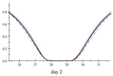
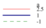
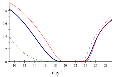
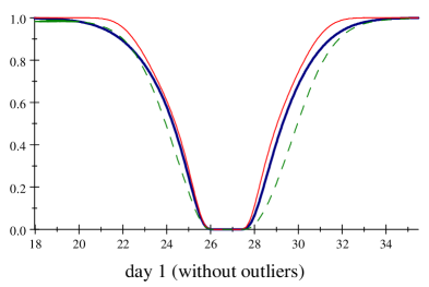
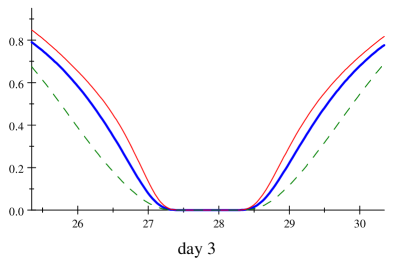
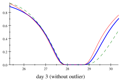
Figure 1: Approximate power functions $\widetilde{\beta}_{n,a}^{1}\left(\mu^{\ast}\right)$ for Newcomb’s measurements for three days.

6 Simulation study

6.1 Evaluation of procedures under normality

In this section, we will pay special attention to a subfamily of $\phi$-divergence measures in (11), the so-called power divergence measures (see Cressie and Read (1984)) for which $\phi(x)\equiv\phi_{\lambda}(x)\in\Phi$ is given by

$$\phi_{\lambda}(x) =\frac{1}{\lambda(1+\lambda)}\left[x^{\lambda+1}-x-\lambda(x-1)\right],\quad\text{if }\lambda(1+\lambda)\neq 0,$$ (31)

$$\phi_{0}(x) =\lim_{\lambda\rightarrow 0}\phi_{\lambda}(x)=x\log x-x+1,$$

$$\phi_{-1}(x) =\lim_{\lambda\rightarrow-1}\phi_{\lambda}(x)=-\log x+x-1.$$

In this case, (12) can be expressed as

$$T_{n}^{\lambda}(\widehat{\boldsymbol{\theta}}_{E,n},\boldsymbol{\theta}_{0}) =\frac{2}{\lambda(1+\lambda)}\left(\sum_{i=1}^{n}(1+\boldsymbol{t}(\boldsymbol{\theta}_{0})^{T}\boldsymbol{g}(\boldsymbol{X}_{i},\boldsymbol{\theta}_{0}))^{\lambda}-\sum_{i=1}^{n}(1+\boldsymbol{t}(\widehat{\boldsymbol{\theta}}_{E,n})^{T}\boldsymbol{g}(\boldsymbol{X}_{i},\widehat{\boldsymbol{\theta}}_{E,n}))^{\lambda}\right)\text{,}\quad\text{if }\lambda(1+\lambda)\neq 0,$$ (32)

$$=2\sum_{i=1}^{n}\log\left(\frac{1+\boldsymbol{t}(\boldsymbol{\theta}_{0})^{T}\boldsymbol{g}(\boldsymbol{X}_{i},\boldsymbol{\theta}_{0})}{1+\boldsymbol{t}(\widehat{\boldsymbol{\theta}}_{E,n})^{T}\boldsymbol{g}(\boldsymbol{X}_{i},\widehat{\boldsymbol{\theta}}_{E,n})}\right)=L_{E,n}(\widehat{\boldsymbol{\theta}}_{E},\boldsymbol{\theta}_{0}),\quad\text{if }\lambda=0,$$

$$=2\left(\sum_{i=1}^{n}\frac{\log(1+\boldsymbol{t}(\widehat{\boldsymbol{\theta}}_{E,n})^{T}\boldsymbol{g}(\boldsymbol{X}_{i},\widehat{\boldsymbol{\theta}}_{E,n})))}{1+\boldsymbol{t}(\widehat{\boldsymbol{\theta}}_{E,n})^{T}\boldsymbol{g}(\boldsymbol{X}_{i},\widehat{\boldsymbol{\theta}}_{E,n})}-\sum_{i=1}^{n}\frac{\log(1+\boldsymbol{t}(\boldsymbol{\theta}_{0})^{T}\boldsymbol{g}(\boldsymbol{X}_{i},\boldsymbol{\theta}_{0})))}{1+\boldsymbol{t}(\boldsymbol{\theta}_{0})^{T}\boldsymbol{g}(\boldsymbol{X}_{i},\boldsymbol{\theta}_{0})}\right)\text{,}\quad\text{if }\lambda=-1.$$

This family of test statistics include several commonly used tests such as the empirical modified Kullback-Leibler statistic ($T_{n}^{\lambda}(\widehat{\boldsymbol{\theta}}_{E,n},\boldsymbol{\theta}_{0})$, with $\lambda=-1$), the empirical Freeman-Tukey statistic ($T_{n}^{\lambda}(\widehat{\boldsymbol{\theta}}_{E,n},\boldsymbol{\theta}_{0})$, with $\lambda=-\frac{1}{2}$), the empirical likelihood ratio test statistic ($T_{n}^{\lambda}(\widehat{\boldsymbol{\theta}}_{E,n},\boldsymbol{\theta}_{0})$, with $\lambda=0$), the empirical Cressie-Read statistic ($T_{n}^{\lambda}(\widehat{\boldsymbol{\theta}}_{E,n},\boldsymbol{\theta}_{0})$, with $\frac{2}{3}$), and the empirical Pearson’s chi-square statistic ($T_{n}^{\lambda}(\widehat{\boldsymbol{\theta}}_{E,n},\boldsymbol{\theta}_{0})$, with $\lambda=1$). Similarly, (13) can be expressed as

$$S_{n}^{\lambda}(\widehat{\boldsymbol{\theta}}_{E,n},\boldsymbol{\theta}_{0}) =\frac{2}{\lambda(1+\lambda)}\left(\sum_{i=1}^{n}\frac{(1+\boldsymbol{t}(\boldsymbol{\theta}_{0})^{T}\boldsymbol{g}(\boldsymbol{X}_{i},\boldsymbol{\theta}_{0}))^{\lambda}}{(1+\boldsymbol{t}(\widehat{\boldsymbol{\theta}}_{E,n})^{T}\boldsymbol{g}(\boldsymbol{X}_{i},\widehat{\boldsymbol{\theta}}_{E,n}))^{\lambda+1}}-n\right)\text{,}\quad\text{if }\lambda(1+\lambda)\neq 0,$$ (33)

$$=2\sum_{i=1}^{n}\frac{1}{1+\boldsymbol{t}(\widehat{\boldsymbol{\theta}}_{E,n})^{T}\boldsymbol{g}(\boldsymbol{X}_{i},\widehat{\boldsymbol{\theta}}_{E,n})}\log\left(\frac{1+\boldsymbol{t}(\boldsymbol{\theta}_{0})^{T}\boldsymbol{g}(\boldsymbol{X}_{i},\boldsymbol{\theta}_{0})}{1+\boldsymbol{t}(\widehat{\boldsymbol{\theta}}_{E,n})^{T}\boldsymbol{g}(\boldsymbol{X}_{i},\widehat{\boldsymbol{\theta}}_{E,n})}\right)\text{,}\quad\text{if }\lambda=0,$$

$$=2\sum_{i=1}^{n}\frac{1}{1+\boldsymbol{t}(\boldsymbol{\theta}_{0})^{T}\boldsymbol{g}(\boldsymbol{X}_{i},\boldsymbol{\theta}_{0})}\log\left(\frac{1+\boldsymbol{t}(\widehat{\boldsymbol{\theta}}_{E,n})^{T}\boldsymbol{g}(\boldsymbol{X}_{i},\widehat{\boldsymbol{\theta}}_{E,n})}{1+\boldsymbol{t}(\boldsymbol{\theta}_{0})^{T}\boldsymbol{g}(\boldsymbol{X}_{i},\boldsymbol{\theta}_{0})}\right)\text{,}\quad\text{if }\lambda=-1.$$

The $r$-dimensional vectors $\boldsymbol{t}(\boldsymbol{\theta}_{0})$ and $\boldsymbol{t}(\widehat{\boldsymbol{\theta}}_{E,n})$ are obtained by solving (6) with $\boldsymbol{\theta}_{0}$ and $\widehat{\boldsymbol{\theta}}_{E,n}$ being specified.

We now examine, through Monte Carlo simulations, the performance of the confidence intervals (CIs) obtained through the empirical power divergence test statistics in (32) and (33) for the choices $\lambda\in\{-1,-\frac{1}{2},0,\frac{2}{3},1\}$, when the sample sizes are small, $n=30,45,60$, and the nominal confidence levels are $90\%$ and $95\%$. Even though the asymptotic distribution is equivalent for the different empirical divergence based statistics, in practice we need to work with finite sample sizes and it is therefore important to compare the CIs based on $T_{n}^{\lambda}(\widehat{\boldsymbol{\theta}}_{E,n},\boldsymbol{\theta}_{0})$ and $S_{n}^{\lambda}(\widehat{\boldsymbol{\theta}}_{E,n},\boldsymbol{\theta}_{0})$, in different scenarios. We focus on the coverage probability and average width of the CIs of a mean based on $5000$ simulated samples under the same setting as Example 1 of Qin and Lawless (1994). In this case, a sample of univariate ($k=1$) i.i.d. random variables, $X_{1},...,X_{n}$, of size $n$ was considered, with mean $\theta$ and variance $\theta^{2}+1$, i.e., $r=2>p=1$ and

$$\boldsymbol{g}(X,\theta)=(g_{1}(X,\theta),g_{2}(X,\theta))^{T}=(X-\theta,X^{2}-2\theta^{2}-1)^{T}.$$

$\mathcal{N}(\theta,\theta^{2}+1)$, $\theta_{0}=0$ $T_{n}^{\lambda}(\widehat{\theta}_{E,n},\theta_{0})$ $S_{n}^{\lambda}(\widehat{\theta}_{E,n},\theta_{0})$ Cov (%) Avw Cov (%) Avw $\lambda$ $n=30$ $90\%$ $-1$ 86.36 0.524 88.35 0.540 $-\frac{1}{2}$ 87.11 0.542 87.98 0.551 $0$ 87.77 0.557 87.64 0.560 $\frac{2}{3}$ 87.46 0.571 86.88 0.570 $1$ 87.19 0.575 86.55 0.573 $95\%$ $-1$ 91.97 0.617 93.85 0.637 $-\frac{1}{2}$ 92.67 0.642 93.77 0.654 $0$ 93.05 0.663 93.48 0.669 $\frac{2}{3}$ 93.05 0.684 92.76 0.684 $1$ 92.88 0.690 92.28 0.689 $\lambda$ $n=45$ $90\%$ $-1$ 87.62 0.445 88.95 0.455 $-\frac{1}{2}$ 88.45 0.457 88.85 0.462 $0$ 88.83 0.469 88.66 0.468 $\frac{2}{3}$ 88.70 0.480 88.11 0.474 $1$ 88.51 0.484 87.81 0.476 $95\%$ $-1$ 93.09 0.526 94.42 0.538 $-\frac{1}{2}$ 93.43 0.544 94.34 0.550 $0$ 94.02 0.559 94.13 0.559 $\frac{2}{3}$ 94.23 0.575 93.51 0.569 $1$ 93.81 0.581 93.22 0.573 $\lambda$ $n=60$ $90\%$ $-1$ 87.19 0.394 88.47 0.401 $-\frac{1}{2}$ 87.86 0.404 88.45 0.405 $0$ 88.36 0.413 88.13 0.409 $\frac{2}{3}$ 88.28 0.421 87.63 0.413 $1$ 88.03 0.425 87.29 0.415 $95\%$ $-1$ 93.22 0.467 93.85 0.475 $-\frac{1}{2}$ 93.45 0.481 93.72 0.483 $0$ 93.95 0.493 93.55 0.489 $\frac{2}{3}$ 93.78 0.505 93.13 0.496 $1$ 93.70 0.509 92.90 0.498                   $\mathcal{N}(\theta,\theta^{2}+1)$, $\theta_{0}=1$ $T_{n}^{\lambda}(\widehat{\theta}_{E,n},\theta_{0})$ $S_{n}^{\lambda}(\widehat{\theta}_{E,n},\theta_{0})$ Cov (%) Avw Cov (%) Avw $\lambda$ $n=30$ $90\%$ $-1$ 83.59 0.627 79.37 0.542 $-\frac{1}{2}$ 84.64 0.635 79.73 0.547 $0$ 85.16 0.642 80.11 0.551 $\frac{2}{3}$ 83.01 0.608 80.51 0.555 $1$ 82.81 0.605 80.39 0.556 $95\%$ $-1$ 88.70 0.728 84.36 0.645 $-\frac{1}{2}$ 89.83 0.740 85.08 0.652 $0$ 90.39 0.749 85.52 0.657 $\frac{2}{3}$ 89.08 0.721 85.88 0.663 $1$ 88.62 0.714 85.82 0.664 $\lambda$ $n=45$ $90\%$ $-1$ 85.13 0.476 84.44 0.460 $-\frac{1}{2}$ 86.03 0.482 85.19 0.464 $0$ 86.46 0.488 85.73 0.468 $\frac{2}{3}$ 86.20 0.485 86.03 0.473 $1$ 86.20 0.487 86.01 0.475 $95\%$ $-1$ 90.37 0.563 89.73 0.546 $-\frac{1}{2}$ 91.12 0.571 90.18 0.553 $0$ 91.45 0.579 90.94 0.559 $\frac{2}{3}$ 91.53 0.580 91.02 0.567 $1$ 91.62 0.582 91.19 0.570 $\lambda$ $n=60$ $90\%$ $-1$ 85.46 0.413 84.91 0.403 $-\frac{1}{2}$ 85.99 0.417 85.46 0.406 $0$ 86.28 0.421 85.80 0.410 $\frac{2}{3}$ 86.37 0.423 85.90 0.415 $1$ 86.39 0.425 86.09 0.417 $95\%$ $-1$ 91.02 0.489 90.83 0.479 $-\frac{1}{2}$ 92.08 0.496 91.80 0.485 $0$ 92.58 0.502 92.25 0.490 $\frac{2}{3}$ 92.92 0.506 92.56 0.498 $1$ 92.86 0.509 92.54 0.501

Table 4: Coverage and average width of $90\%$ and $95\%$ confidence intervals.

In the present study, we have considered an additional sample of size $n=45$, compared to those of Qin and Lawless (1994). For constructing the test statistic, an unknown distribution of $X_{i}$ is assumed, but for this simulation study, normally distributed random variables were taken with $\theta_{0}\in\{0,1\}$. It is important to mention here that Baggerly (1998) studied the coverage probabilities for the normal distribution, but only for the family of statistics in (32). The results of the simulation study are summarized in Table 4 and Figure 2 for the empirical power divergence test statistics in (32) and (33) for two different samples when the nominal confidence level is $95\%$. In Figure 2, it can be seen that the confidence intervals based on both statistics, $T_{n}^{\lambda}(\widehat{\theta}_{E,n},\theta_{0})$ and $S_{n}^{\lambda}(\widehat{\theta}_{E,n},\theta_{0})$, with small values of $\lambda\in\{-1,-\frac{1}{2},0,\frac{2}{3},1\}$ tend to be narrower in width, and this is also seen in the simulation results of Table 4. In fact, the simulation study of Baggerly showed that $T_{n}^{-1}(\widehat{\theta}_{E,n},\theta_{0})$ had the worst coverage probability, and this is also seen in the present simulation study. This is in accordance with the results obtained for two specific samples analyzed in Figure 2. The smallest average width of confidence intervals is obtained for $S_{n}^{-1}(\widehat{\theta}_{E,n},\theta_{0})$, which is the so-called empirical modified likelihood ratio test statistic or empirical minimum discrimination information statistic (see Gokhale and Kullback, 1978), and this might explain, when $\theta_{0}=0$, the low coverage probability as well. Often, the coverage probability closest to the nominal level is also obtained for the same test statistics, $S_{n}^{-1}(\widehat{\theta}_{E,n},\theta_{0})$ when $\theta_{0}=1$ but the empirical likelihood ratio test has a closer coverage probability when $\theta_{0}=0$. When both characteristics of a CI, viz., average width and coverage probability, are taken into account, the empirical modified likelihood ratio test statistic, $S_{n}^{-1}(\widehat{\theta}_{E,n},\theta_{0})$, is a good compromise and it turns out to be the best for $\theta_{0}=0$ in all the cases considered. Finally, another important feature seen in Figure 2 is that even though the support of the asymptotic distribution of the test statistics is strictly positive, it is possible to find samples for which $T_{n}^{\lambda}(\widehat{\theta}_{E,n},\theta_{0})$ is negative, while $S_{n}^{\lambda}(\widehat{\theta}_{E,n},\theta_{0})$ is always strictly positive. This usually happens when $\widehat{\theta}_{E,n}$ is very close to $\theta_{0}$.

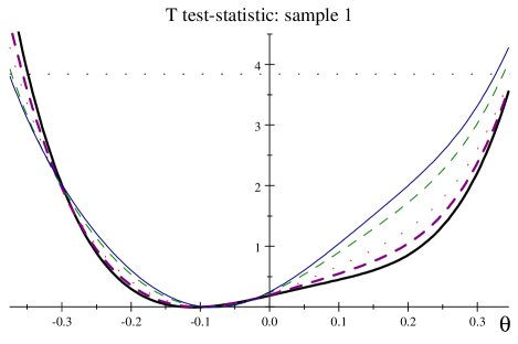
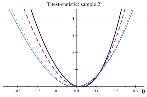
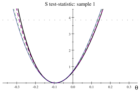
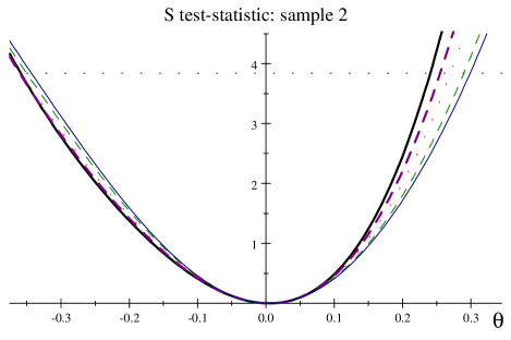
Figure 2: Test statistics for samples 1 and 2 of size 30 from the standard normal population.

6.2 Robustness of procedures to contamination in the data

We conducted a simulation study using the same design as in the preceding subsection, but by considering $\frac{15}{100}\%$ of shifted observations in each sample: $2$ shifted observations out of $30$ in the sample, $3$ shifted observations out of $45$, $4$ shifted observations out of $60$. The underlying distribution for shifted observations is taken to be $\mathcal{N}(\theta+\sqrt{\theta^{2}+1},\theta^{2}+1)$, given that $\mathcal{N}(\theta,\theta^{2}+1)$ is the true distribution. Therefore, the shifted observations follow $\mathcal{N}(1,1)$ distribution when the true distribution is $\mathcal{N}(0,1)$, while they follow $\mathcal{N}(2.4142,2)$ distribution when the true distribution is $\mathcal{N}(1,2)$. In Table 5, the results of introducing $\frac{15}{100}\%$ of shifted observations is shown. Our interest is focused on identifying the statistics that are less sensitive (robust statistics with respect to shifted observations) as well as those that are quite sensitive (non-robust statistics with respect to shifted observations). As pointed out in Remark 6, all the test-statistics have the same infinitesimal robustness, so the differences in robustness could be atributable to the magnitude of the shift. When $\theta_{0}=0$, the best statistics with shifted observations are exactly the same as ones without shifted observations, but when the dispersion of the data is higher, i.e. $\theta_{0}=1$, the closest coverage probability to the nominal level is not for the empirical likelihood ratio test; we further observe that $T_{n}^{\lambda}(\widehat{\theta}_{E,n},\theta_{0})$ and $S_{n}^{\lambda}(\widehat{\theta}_{E,n},\theta_{0})$ not only have the narrowest CIs but also the highest coverage probabilities. This means that the empirical modified likelihood ratio test statistic, $S_{n}^{-1}(\widehat{\theta}_{E,n},\theta_{0})$, is a robust statistic with respect to shifted observations in comparison to the empirical likelihood ratio test, with respect to the coverage probability and width of CIs. This also agrees with the conclusion obtained from Table 3.

$\mathcal{N}(\theta,\theta^{2}+1)$, $\theta_{0}=0$ $T_{n}^{\lambda}(\widehat{\theta}_{E,n},\theta_{0})$ $S_{n}^{\lambda}(\widehat{\theta}_{E,n},\theta_{0})$ Cov (%) Avw Cov (%) Avw $\lambda$ $n=30$ $90\%$ $-1$ 83.54 0.553 84.47 0.542 $-\frac{1}{2}$ 84.39 0.568 84.15 0.552 $0$ 84.51 0.580 83.84 0.560 $\frac{2}{3}$ 84.17 0.590 83.15 0.569 $1$ 83.80 0.592 82.61 0.572 $95\%$ $-1$ 90.27 0.652 90.70 0.639 $-\frac{1}{2}$ 91.00 0.673 90.65 0.655 $0$ 91.40 0.691 90.05 0.670 $\frac{2}{3}$ 90.90 0.707 89.07 0.684 $1$ 90.33 0.711 88.65 0.689 $\lambda$ $n=45$ $90\%$ $-1$ 83.59 0.471 83.08 0.457 $-\frac{1}{2}$ 84.10 0.479 83.08 0.463 $0$ 84.24 0.486 82.75 0.469 $\frac{2}{3}$ 83.63 0.492 82.03 0.474 $1$ 83.32 0.493 81.62 0.476 $95\%$ $-1$ 90.30 0.557 90.59 0.541 $-\frac{1}{2}$ 91.10 0.570 90.18 0.551 $0$ 91.41 0.581 89.81 0.560 $\frac{2}{3}$ 91.06 0.590 89.22 0.570 $1$ 90.55 0.593 88.56 0.573 $\lambda$ $n=60$ $90\%$ $-1$ 83.15 0.418 82.33 0.402 $-\frac{1}{2}$ 83.56 0.424 82.14 0.406 $0$ 83.65 0.428 81.73 0.410 $\frac{2}{3}$ 83.34 0.431 81.28 0.414 $1$ 82.86 0.431 80.93 0.415 $95\%$ $-1$ 90.10 0.495 89.30 0.477 $-\frac{1}{2}$ 90.39 0.505 89.12 0.484 $0$ 90.17 0.512 88.89 0.490 $\frac{2}{3}$ 89.55 0.517 88.34 0.497 $1$ 89.43 0.518 87.92 0.499                    $\mathcal{N}(\theta,\theta^{2}+1)$, $\theta_{0}=1$ $T_{n}^{\lambda}(\widehat{\theta}_{E,n},\theta_{0})$ $S_{n}^{\lambda}(\widehat{\theta}_{E,n},\theta_{0})$ Cov (%) Avw Cov (%) Avw $\lambda$ $n=30$ $90\%$ $-1$ 85.09 0.564 85.58 0.575 $-\frac{1}{2}$ 85.13 0.571 85.37 0.580 $0$ 84.43 0.577 84.72 0.584 $\frac{2}{3}$ 83.11 0.582 83.62 0.589 $1$ 82.31 0.583 83.19 0.590 $95\%$ $-1$ 91.13 0.669 91.50 0.683 $-\frac{1}{2}$ 91.28 0.680 91.42 0.691 $0$ 90.97 0.688 90.89 0.697 $\frac{2}{3}$ 89.87 0.695 90.13 0.702 $1$ 89.13 0.696 89.56 0.704 $\lambda$ $n=45$ $90\%$ $-1$ 86.25 0.473 86.50 0.479 $-\frac{1}{2}$ 85.96 0.479 85.90 0.483 $0$ 85.14 0.484 85.57 0.488 $\frac{2}{3}$ 84.05 0.490 84.30 0.493 $1$ 83.15 0.493 83.56 0.496 $95\%$ $-1$ 92.48 0.562 92.25 0.569 $-\frac{1}{2}$ 92.09 0.570 92.25 0.576 $0$ 91.66 0.578 91.72 0.583 $\frac{2}{3}$ 90.44 0.588 90.63 0.592 $1$ 89.46 0.592 89.85 0.595 $\lambda$ $n=60$ $90\%$ $-1$ 85.22 0.416 85.24 0.419 $-\frac{1}{2}$ 84.61 0.420 84.67 0.423 $0$ 83.95 0.425 83.91 0.427 $\frac{2}{3}$ 82.49 0.431 82.66 0.432 $1$ 81.70 0.434 82.03 0.435 $95\%$ $-1$ 91.93 0.494 91.62 0.498 $-\frac{1}{2}$ 91.41 0.501 91.27 0.504 $0$ 90.29 0.508 90.35 0.510 $\frac{2}{3}$ 89.23 0.517 89.35 0.519 $1$ 88.42 0.522 88.96 0.523

Table 5: Coverage probability and average width of $90\%$ and $95\%$ confidence intervals with data contaminated by shifted observations.

7 Testing for a composite null hypothesis

Now, let us consider the problem of testing the composite null hypothesis

$$H_{0}:\boldsymbol{c}(\boldsymbol{\theta})\boldsymbol{=0}_{q}.$$ (34)

The rest of this section, proceeds as follows. In Section 7.1, we introduce the empirical phi-divergence test statistic for the composite null hypothesis in (34). Section 7.2 is devoted to the asymptotic results. In Section 7.3, we present some results regarding the power function of the family of empirical test statistics proposed here. In Section 7.4, a simulation study is carried out to evaluate the performance of the proposed test procedure in comparison to some other tests.

7.1 Empirical phi-divergence test statistics

In the following, we shall assume as in Qin and Lawless (1995), that the unknown parameter vector $\boldsymbol{\theta}$ is defined through $r=p$ estimating functions, given in (1). With regard to (34), we shall assume that $\boldsymbol{c}:$ $\mathbb{R}^{p}\mathbb{\rightarrow R}^{q}$ is a vector-valued function such that the $q\times p$ matrix $\boldsymbol{C}$$\left(\boldsymbol{\theta}\right)=\frac{\partial\boldsymbol{c(\theta)}}{\partial\boldsymbol{\theta}^{T}}$ exists and is continuous at $\boldsymbol{\theta}$ and that $\mathrm{rank}($$\boldsymbol{C}$$\left(\boldsymbol{\theta}\right))=q$ ($q\leq p$). We denote by $\widetilde{\boldsymbol{\theta}}_{E,n}$ the empirical restricted maximum likelihood estimator of $\boldsymbol{\theta}$, obtained by minimizing $\ell_{E,n}(\boldsymbol{\theta})=-\sum_{i=1}^{n}\log\left[1+\boldsymbol{t}(\boldsymbol{\theta})^{T}\boldsymbol{g}(\boldsymbol{X}_{i},\boldsymbol{\theta})\right]$, subject to $\sum_{i=1}^{n}p_{i}\left(\boldsymbol{\theta}\right)\boldsymbol{g}(\boldsymbol{X}_{i},\boldsymbol{\theta})=\boldsymbol{0}_{r}$ and $\boldsymbol{c}$$\boldsymbol{(\theta)=0}_{q}$, i.e., (6) or

$$\boldsymbol{\xi}_{1n}\left(\boldsymbol{\theta},\boldsymbol{\boldsymbol{t}(\boldsymbol{\theta})},\boldsymbol{\nu}\right)=\boldsymbol{0}_{p}\text{,}$$ (35)

where

$$\boldsymbol{\xi}_{1n}\left(\boldsymbol{\theta},\boldsymbol{\boldsymbol{t}(\boldsymbol{\theta})},\boldsymbol{\nu}\right)=\boldsymbol{\xi}_{1n}\left(\boldsymbol{\theta},\boldsymbol{\boldsymbol{t}(\boldsymbol{\theta})}\right)=\frac{1}{n}\sum\limits_{i=1}^{n}\frac{1}{1+\boldsymbol{t}(\boldsymbol{\theta})^{T}\boldsymbol{g}(\boldsymbol{X}_{i},\boldsymbol{\theta})}\boldsymbol{g}(\boldsymbol{X}_{i},\boldsymbol{\theta})$$

provides $\boldsymbol{t}(\boldsymbol{\theta})$ in terms of $\boldsymbol{\theta}$. Upon using the Lagrange multiplier method, once again, we have

$$\zeta_{E,n}(\boldsymbol{\theta},\boldsymbol{\boldsymbol{t}(\boldsymbol{\theta})},\boldsymbol{\nu})=\frac{1}{n}\ell_{E,n}(\boldsymbol{\theta)}+\boldsymbol{\nu}^{T}\boldsymbol{c(\theta)},$$

where $\boldsymbol{\nu}$ is a $q$-dimensional vector of Lagrange multipliers, and differentiating $\zeta_{E,n}(\boldsymbol{\theta},\boldsymbol{\boldsymbol{t}(\boldsymbol{\theta})},\boldsymbol{\nu})$ with respect to $\boldsymbol{\theta}$ and $\boldsymbol{\nu}$, we obtain

$$\boldsymbol{\xi}_{2n}\left(\boldsymbol{\theta},\boldsymbol{\boldsymbol{t}(\boldsymbol{\theta})},\boldsymbol{\nu}\right) =\frac{1}{n}\sum\limits_{i=1}^{n}\frac{1}{1+\boldsymbol{t}(\boldsymbol{\theta})^{T}\boldsymbol{g}(\boldsymbol{X}_{i},\boldsymbol{\theta})}\boldsymbol{G}_{\boldsymbol{X}_{i}}(\boldsymbol{\theta})^{T}\boldsymbol{t}(\boldsymbol{\theta})+\mathbf{C}(\boldsymbol{\theta})\boldsymbol{{}^{T}\nu},$$

$$\boldsymbol{\xi}_{3n}\left(\boldsymbol{\theta},\boldsymbol{\boldsymbol{t}(\boldsymbol{\theta})},\boldsymbol{\nu}\right) =\boldsymbol{\xi}_{3n}\left(\boldsymbol{\theta}\right)=\boldsymbol{c(\theta)}.$$

Therefore, $(\widetilde{\boldsymbol{\theta}}_{E,n}^{T},\widetilde{\boldsymbol{\nu}}_{E,n}^{T})^{T}$ is obtained as the solution of (35) and

$$\boldsymbol{\xi}_{2n}\left(\boldsymbol{\theta,\boldsymbol{t}(\boldsymbol{\theta}),\nu}\right)=\boldsymbol{0}_{p}\text{,}\boldsymbol{\qquad\xi}_{3n}\left(\boldsymbol{\theta,\boldsymbol{t}(\boldsymbol{\theta}),\nu}\right)=\boldsymbol{0}_{q}\text{,}$$ (36)

and conditions (3) and (5) must be also satisfied.

The empirical likelihood ratio test for testing (34) has the expression

$$L_{E,n}(\widehat{\boldsymbol{\theta}}_{E,n},\widetilde{\boldsymbol{\theta}}_{E,n})=2\ell_{E,n}(\widehat{\boldsymbol{\theta}}_{E,n})-2\ell_{E,n}(\widetilde{\boldsymbol{\theta}}_{E,n}),$$ (37)

where $\widehat{\boldsymbol{\theta}}_{E,n}$ is the empirical maximum likelihood estimator of the parameter $\boldsymbol{\theta}$, defined in Section 1 (case $r=p$), for which $\ell_{E,n}(\widehat{\boldsymbol{\theta}}_{E})=0$. Taking into account the results stated in Section 1 for $r=p$, we have $F_{n}=F_{n,\widehat{\boldsymbol{\theta}}_{E,n}}$, and so it is easy to show that the expression in (37) can be written as

$$L_{E,n}(\widehat{\boldsymbol{\theta}}_{E,n},\widetilde{\boldsymbol{\theta}}_{E,n})=2n\left(D_{Kullback}(F_{n},F_{n,\widetilde{\boldsymbol{\theta}}_{E,n}})-D_{Kullback}(F_{n},F_{n,\widehat{\boldsymbol{\theta}}_{E,n}})\right)=2nD_{Kullback}(F_{n,\widehat{\boldsymbol{\theta}}_{E,n}},F_{n,\widetilde{\boldsymbol{\theta}}_{E,n}}).$$

Defining a family of empirical phi-divergence test statistics for testing the hypothesis in (34), we have

$$T_{n}^{\phi}(\widehat{\boldsymbol{\theta}}_{E,n},\widetilde{\boldsymbol{\theta}}_{E,n}) =\frac{2n}{\phi^{\prime\prime}(1)}\left(D_{\phi}(F_{n},F_{n,\widetilde{\boldsymbol{\theta}}_{E,n}})-D_{\phi}(F_{n},F_{n,\widehat{\boldsymbol{\theta}}_{E,n}})\right),$$

$$S_{n}^{\phi}(\widehat{\boldsymbol{\theta}}_{E,n},\widetilde{\boldsymbol{\theta}}_{E,n}) =\frac{2n}{\phi^{\prime\prime}(1)}D_{\phi}(F_{n,\widehat{\boldsymbol{\theta}}_{E,n}},F_{n,\widetilde{\boldsymbol{\theta}}_{E,n}})$$

where the $\phi$-divergence measures are as defined in (11). Since $F_{n}=F_{n,\widehat{\boldsymbol{\theta}}_{E,n}}$, both families of empirical phi-divergence test statistics are equivalent and taking into account (13) and $\boldsymbol{t}(\widehat{\boldsymbol{\theta}}_{E,n})=\boldsymbol{0}_{p}$, we have

$$T_{n}^{\phi}(\widehat{\boldsymbol{\theta}}_{E,n},\widetilde{\boldsymbol{\theta}}_{E,n}) =S_{n}^{\phi}(\widehat{\boldsymbol{\theta}}_{E,n},\widetilde{\boldsymbol{\theta}}_{E,n})$$

$$=\frac{2}{\phi^{\prime\prime}(1)}\sum\limits_{i=1}^{n}\frac{\phi\left(1+\boldsymbol{t}(\widetilde{\boldsymbol{\theta}}_{E,n})^{T}\boldsymbol{g}(\boldsymbol{x}_{i},\widetilde{\boldsymbol{\theta}}_{E,n})\right)}{1+\boldsymbol{t}(\widetilde{\boldsymbol{\theta}}_{E,n})^{T}\boldsymbol{g}(\boldsymbol{x}_{i},\widetilde{\boldsymbol{\theta}}_{E,n})}.$$ (38)

7.2 Asymptotic null distributions

Under the same conditions of Theorem 3 and the conditions given in Section 7.1 for $\boldsymbol{c}(\boldsymbol{\theta})$, it is assumed that there exists a neighbourhood of $\boldsymbol{\theta}_{0}$ in which $\left\|\frac{\partial\boldsymbol{C}(\boldsymbol{\theta})}{\partial\boldsymbol{\theta}}\right\|$ is bounded by some some constant, we have

$$\sqrt{n}\left(\begin{array}[c]{c}\widetilde{\boldsymbol{\theta}}_{E,n}-\boldsymbol{\theta}_{0}\\ \widetilde{\boldsymbol{\nu}}_{E,n}\end{array}\right)\underset{n\rightarrow\infty}{\overset{\mathcal{L}}{\rightarrow}}\mathcal{N}\left(\boldsymbol{0}_{p+q},\left(\begin{array}[c]{cc}\boldsymbol{P}\left(\boldsymbol{\theta}_{0}\right)&\boldsymbol{0}_{p\times q}\\ \boldsymbol{0}_{q\times p}&\boldsymbol{Q}\left(\boldsymbol{\theta}_{0}\right)\end{array}\right)\right),$$ (39)

where $\boldsymbol{\theta}_{0}$ is the true value of the parameter $\boldsymbol{\theta}$ and

$$\boldsymbol{P\left(\boldsymbol{\theta}_{0}\right)} \boldsymbol{=V\left(\boldsymbol{\theta}_{0}\right)}-\boldsymbol{V\left(\boldsymbol{\theta}_{0}\right)C}\left(\boldsymbol{\theta}_{0}\right)^{T}\boldsymbol{Q\left(\boldsymbol{\theta}_{0}\right)C\left(\boldsymbol{\theta}_{0}\right)V\left(\boldsymbol{\theta}_{0}\right)},$$ (40)

$$\boldsymbol{Q}\left(\boldsymbol{\theta}_{0}\right) =(\boldsymbol{C\left(\boldsymbol{\theta}_{0}\right)V\left(\boldsymbol{\theta}_{0}\right)C}\left(\boldsymbol{\theta}_{0}\right)^{T})^{-1}.$$ (41)

This result is derived by taking into account, the facts that

$$\sqrt{n}(\widetilde{\boldsymbol{\theta}}_{E,n}-\boldsymbol{\theta}_{0}) =-\boldsymbol{S}_{12}^{-1}\left(\boldsymbol{\theta}_{0}\right)\sqrt{n}\boldsymbol{\bar{g}}_{n}(\boldsymbol{\theta}_{0})-\boldsymbol{V}\left(\boldsymbol{\theta}_{0}\right)\boldsymbol{C}\left(\boldsymbol{\theta}_{0}\right)^{T}\sqrt{n}\widetilde{\boldsymbol{\nu}}_{E,n}+o_{p}(1),$$ (42)

$$\sqrt{n}\widetilde{\boldsymbol{\nu}}_{E,n} =-\boldsymbol{Q\left(\boldsymbol{\theta}_{0}\right)C\left(\boldsymbol{\theta}_{0}\right)S}_{12}^{-1}\left(\boldsymbol{\theta}_{0}\right)\sqrt{n}\boldsymbol{\bar{g}}_{n}(\boldsymbol{\theta}_{0})+o_{p}(1).$$ (43)

For a complete proof, one may refer to Qin and Lawless (1995).

Theorem 13

Under $H_{0}$ in (34) and the assumptions above, we have

$$T_{n}^{\phi}(\widehat{\boldsymbol{\theta}}_{E,n},\widetilde{\boldsymbol{\theta}}_{E,n})\overset{\mathcal{L}}{\underset{n\rightarrow\infty}{\longrightarrow}}\chi_{q}^{2}.$$ (44)

Proof. Let us consider the function

$$\ell_{\phi}\left(\boldsymbol{t}\right)=\frac{1}{n}\sum\limits_{i=1}^{n}\frac{\phi(1+\boldsymbol{t}^{T}\boldsymbol{g}(\boldsymbol{x}_{i},\widetilde{\boldsymbol{\theta}}_{E,n}))}{1+\boldsymbol{t}^{T}\boldsymbol{g}(\boldsymbol{x}_{i},\widetilde{\boldsymbol{\theta}}_{E,n})}.$$

A second-order Taylor expansion of $\ell_{\phi}(\widetilde{\boldsymbol{t}})$ around $\boldsymbol{0}_{p}$, with $\widetilde{\boldsymbol{t}}=\boldsymbol{t}(\widetilde{\boldsymbol{\theta}}_{E,n})$, gives

$$T_{n}^{\phi}(\widehat{\boldsymbol{\theta}}_{E,n},\widetilde{\boldsymbol{\theta}}_{E,n})=\frac{2n\ell_{\phi}(\widetilde{\boldsymbol{t}})}{\phi^{\prime\prime}\left(1\right)}=n\boldsymbol{t}(\widetilde{\boldsymbol{\theta}}_{E,n})^{T}\boldsymbol{S}_{11}(\widetilde{\boldsymbol{\theta}}_{E,n})\boldsymbol{t}(\widetilde{\boldsymbol{\theta}}_{E,n})+o\left(||\sqrt{n}\boldsymbol{t}(\widetilde{\boldsymbol{\theta}}_{E,n})||^{2}\right).$$

But,

$$\sqrt{n}\boldsymbol{t}(\widetilde{\boldsymbol{\theta}}_{E,n})=\sqrt{n}\boldsymbol{S}_{11}^{-1}\left(\boldsymbol{\theta}_{0}\right)\boldsymbol{\bar{g}}_{n}(\widetilde{\boldsymbol{\theta}}_{E,n})+o_{p}(\boldsymbol{1}_{r}),$$

and

$$\boldsymbol{\bar{g}}_{n}(\widetilde{\boldsymbol{\theta}}_{E,n}) =\boldsymbol{\bar{g}}_{n}(\boldsymbol{\theta}_{0})+\frac{\partial}{\partial\boldsymbol{\theta}^{T}}\left.\boldsymbol{\bar{g}}_{n}\left(\boldsymbol{\theta}\right)\right|_{\boldsymbol{\theta}=\boldsymbol{\theta}_{0}}(\widetilde{\boldsymbol{\theta}}_{E,n}-\boldsymbol{\theta}_{0})+o_{p}(n^{-1/2}\boldsymbol{1}_{r})$$

$$=\boldsymbol{\bar{g}}_{n}(\boldsymbol{\theta}_{0})+\boldsymbol{S}_{12}\left(\boldsymbol{\theta}_{0}\right)(\widetilde{\boldsymbol{\theta}}_{E,n}-\boldsymbol{\theta}_{0})+o_{p}(n^{-1/2}\boldsymbol{1}_{r})$$

$$=\boldsymbol{S}_{12}\left(\boldsymbol{\theta}_{0}\right)\boldsymbol{V}\left(\boldsymbol{\theta}_{0}\right)\boldsymbol{C}\left(\boldsymbol{\theta}_{0}\right)^{T}\widetilde{\boldsymbol{\nu}}_{E,n}+o_{p}(n^{-1/2}\boldsymbol{1}_{r}).$$

By the strong law of large numbers, $\frac{\partial}{\partial\boldsymbol{\theta}^{T}}\left.\boldsymbol{\bar{g}}_{n}\left(\boldsymbol{\theta}\right)\right|_{\boldsymbol{\theta}=\boldsymbol{\theta}_{0}}\overset{a.s.}{\underset{n\rightarrow\infty}{\longrightarrow}}\boldsymbol{S}_{12}\left(\boldsymbol{\theta}_{0}\right)$, and so (42) can be rewritten as

$$\boldsymbol{S}_{12}\left(\boldsymbol{\theta}_{0}\right)(\widetilde{\boldsymbol{\theta}}_{E,n}-\boldsymbol{\theta}_{0})=-\boldsymbol{\bar{g}}_{n}(\boldsymbol{\theta}_{0})-\boldsymbol{S}_{12}\left(\boldsymbol{\theta}_{0}\right)\boldsymbol{V}\left(\boldsymbol{\theta}_{0}\right)\boldsymbol{C}\left(\boldsymbol{\theta}_{0}\right)^{T}\widetilde{\boldsymbol{\nu}}_{E,n}+o_{p}(n^{-1/2}\boldsymbol{1}_{r}).$$

Consequently,

$$T_{n}^{\phi}(\widehat{\boldsymbol{\theta}}_{E,n},\widetilde{\boldsymbol{\theta}}_{E,n})=\left(\sqrt{n}\widetilde{\boldsymbol{\nu}}_{E,n}\right)^{T}\boldsymbol{Q}^{-1}\left(\boldsymbol{\theta}_{0}\right)\sqrt{n}\widetilde{\boldsymbol{\nu}}_{E,n}+o_{p}(1),$$ (45)

with $\sqrt{n}\widetilde{\boldsymbol{\nu}}_{E,n}\underset{n\rightarrow\infty}{\overset{\mathcal{L}}{\rightarrow}}\mathcal{N}\left(\boldsymbol{0}_{q},\boldsymbol{Q}\left(\boldsymbol{\theta}_{0}\right)\right)$, which means that (44) holds.   

7.3 Approximations of the power function

Assume that $\boldsymbol{\theta}^{\ast}\notin\Theta_{0}$ is the true value of the unknown parameter so that $\widehat{\boldsymbol{\theta}}_{E,n}\underset{n\rightarrow\infty}{\overset{a.s.}{\rightarrow}}\boldsymbol{\theta}^{\ast}$, and that there exists a $\boldsymbol{\theta}_{0}\in\Theta_{0}$ such that the restricted empirical maximum likelihood estimator satisfies $\widetilde{\boldsymbol{\theta}}_{E,n}\underset{n\rightarrow\infty}{\overset{a.s.}{\rightarrow}}\boldsymbol{\theta}_{0}$. Then, we have

$$\sqrt{n}\left(\left(\begin{array}[c]{c}\widehat{\boldsymbol{\theta}}_{E,n}\\ \widetilde{\boldsymbol{\theta}}_{E,n}\end{array}\right)-\left(\begin{array}[c]{c}\boldsymbol{\theta}^{\ast}\\ \boldsymbol{\theta}_{0}\end{array}\right)\right)\underset{n\rightarrow\infty}{\overset{\mathcal{L}}{\rightarrow}}\mathcal{N}\left(\left(\begin{array}[c]{c}\boldsymbol{0}_{p}\\ \boldsymbol{0}_{p}\end{array}\right),\left(\begin{array}[c]{cc}\boldsymbol{V}\left(\boldsymbol{\theta}_{0}\right)&\boldsymbol{A}_{12}\left(\boldsymbol{\theta}^{\ast},\boldsymbol{\theta}_{0}\right)\\ \boldsymbol{A}_{12}\left(\boldsymbol{\theta}^{\ast},\boldsymbol{\theta}_{0}\right)^{T}&\boldsymbol{P(\theta}_{0})\end{array}\right)\right),$$ (46)

where $\boldsymbol{A}_{12}\left(\boldsymbol{\theta}^{\ast},\boldsymbol{\theta}_{0}\right)$ is a $q\times q$ matrix.

Theorem 14

Under the conditions stated above, we have

$$\sqrt{n}\left(D_{\phi}(\widehat{\boldsymbol{\theta}}_{E,n},\widetilde{\boldsymbol{\theta}}_{E,n})-D_{\phi}(\boldsymbol{\theta}^{\ast},\boldsymbol{\theta}_{0})\right)\underset{n\rightarrow\infty}{\overset{\mathcal{L}}{\rightarrow}}\mathcal{N}\left(0,\varsigma_{\phi}^{2}(\boldsymbol{\theta}^{\ast},\boldsymbol{\theta}_{0})\right),$$

where

$$\varsigma_{\phi}^{2}\left(\boldsymbol{\theta}^{\ast},\boldsymbol{\theta}_{0}\right)=\boldsymbol{\tau}_{\phi}^{T}\boldsymbol{\left(\boldsymbol{\theta}^{\ast},\boldsymbol{\theta}_{0}\right)V}\left(\boldsymbol{\theta}_{0}\right)\boldsymbol{\tau}_{\phi}\boldsymbol{\left(\boldsymbol{\theta}^{\ast},\boldsymbol{\theta}_{0}\right)+}2\boldsymbol{\boldsymbol{\tau}_{\phi}\boldsymbol{\left(\boldsymbol{\theta}^{\ast},\boldsymbol{\theta}_{0}\right)}}^{T}\boldsymbol{A}_{12}\left(\boldsymbol{\theta}^{\ast},\boldsymbol{\theta}_{0}\right)\boldsymbol{\iota}_{\phi}\boldsymbol{\left(\boldsymbol{\theta}^{\ast},\boldsymbol{\theta}_{0}\right)}+\boldsymbol{\iota}_{\phi}\boldsymbol{\left(\boldsymbol{\theta}^{\ast},\boldsymbol{\theta}_{0}\right)}^{T}\boldsymbol{P(\theta}_{0})\boldsymbol{\iota}_{\phi}\boldsymbol{\left(\boldsymbol{\theta}^{\ast},\boldsymbol{\theta}_{0}\right),}$$

with $\boldsymbol{\tau}_{\phi}\boldsymbol{\left(\boldsymbol{\theta}^{\ast},\boldsymbol{\theta}_{0}\right)}$ given by (24) and

$$\boldsymbol{\iota}_{\phi}\boldsymbol{\left(\boldsymbol{\theta}^{\ast},\boldsymbol{\theta}_{0}\right)=}(\iota_{1}^{\phi}\left(\boldsymbol{\theta}^{\ast},\boldsymbol{\boldsymbol{\theta}_{0}}\right),...,\iota_{p}^{\phi}\left(\boldsymbol{\theta}^{\ast},\boldsymbol{\boldsymbol{\theta}_{0}}\right))^{T}=\left.\frac{\partial D_{\phi}\left(\boldsymbol{\theta}^{\ast},\boldsymbol{\vartheta}\right)}{\partial\boldsymbol{\vartheta}}\right|_{\boldsymbol{\vartheta}=\boldsymbol{\theta}_{0}}.$$

Remark 15

Based on Theorem 14, we get an approximation of the power function at $\boldsymbol{\theta}^{\ast}$ as

$$\beta_{n,\phi}^{1}(\boldsymbol{\theta}^{\ast},\boldsymbol{\boldsymbol{\theta}_{0}}) =P_{\boldsymbol{\theta}^{\ast}}(T_{n}^{\phi}(\widehat{\boldsymbol{\theta}}_{E,n},\widetilde{\boldsymbol{\theta}}_{E,n})>\chi_{q,\alpha}^{2})$$

$$=1-\Phi\left(\frac{\sqrt{n}}{\varsigma_{\phi}\left(\boldsymbol{\theta}^{\ast},\boldsymbol{\theta}_{0}\right)}\left(\frac{\phi^{\prime\prime}\left(1\right)}{2n}\chi_{q,\alpha}^{2}-D_{\phi}\left(F_{n,\boldsymbol{\theta}^{\ast}},F_{n,\boldsymbol{\theta}_{0}}\right)\right)\right).$$

If some alternative $\boldsymbol{\theta}^{\ast}\neq\boldsymbol{\theta}_{0}$ is the true parameter, then the probability of rejecting $\boldsymbol{\theta}_{0}$ with the rejection rule $T_{n}^{\phi}(\widehat{\boldsymbol{\theta}}_{E,n},\widetilde{\boldsymbol{\theta}}_{E,n})>\chi_{q,\alpha}^{2}$, for a fixed significance level $\alpha$, tends to one as $n\rightarrow\infty.$ Thus, the test is consistent in the sense of Fraser (1957).

We may also find an approximation to the power of $T_{n}^{\phi}(\widehat{\boldsymbol{\theta}}_{E,n},\widetilde{\boldsymbol{\theta}}_{E,n})$ at an alternative hypothesis close to the null hypothesis. Let $\boldsymbol{\theta}_{n}\in\Theta-\Theta_{0}$ be a given alternative, and let $\boldsymbol{\theta}_{0}$ be the element in $\Theta_{0}$ closest to $\boldsymbol{\theta}_{n}$ in terms of Euclidean distance. In order to introduce contiguous alternative hypotheses, we may consider a fixed $\boldsymbol{f}$ $\in\mathbb{R}^{p}$ and allow $\boldsymbol{\theta}_{n}$ to tend to $\boldsymbol{\theta}_{0}$ as $n$ increases in the following manner:

$$H_{1,n}:\boldsymbol{\theta}_{n}=\boldsymbol{\theta}_{0}+n^{-1/2}\boldsymbol{f.}$$ (47)

Theorem 16

Under the assumptions of Theorem 13 and $H_{1,n}$ given in (47), we have

$$T_{n}^{\phi}(\widehat{\boldsymbol{\theta}}_{E,n},\widetilde{\boldsymbol{\theta}}_{E,n})\overset{\mathcal{L}}{\underset{n\rightarrow\infty}{\longrightarrow}}\chi_{q}^{2}(\varrho(\boldsymbol{\theta}_{0})),$$ (48)

where $\varrho(\boldsymbol{\theta}_{0})=\boldsymbol{f}^{T}\boldsymbol{C\left(\boldsymbol{\theta}_{0}\right)}^{T}\boldsymbol{Q\left(\boldsymbol{\theta}_{0}\right)C\left(\boldsymbol{\theta}_{0}\right)f}$.

Proof. If we substitute (43) into (45), we obtain

$$T_{n}^{\phi}(\widehat{\boldsymbol{\theta}}_{E,n},\widetilde{\boldsymbol{\theta}}_{E,n})=\sqrt{n}\boldsymbol{\bar{g}}_{n}^{T}\left(\boldsymbol{\theta}_{0}\right)\boldsymbol{S}_{12}^{-1}\left(\boldsymbol{\theta}_{0}\right)\boldsymbol{C}(\boldsymbol{\boldsymbol{\theta}_{0}})\boldsymbol{{}^{T}Q}(\boldsymbol{\boldsymbol{\theta}_{0}})\boldsymbol{C}(\boldsymbol{\boldsymbol{\theta}_{0}})\boldsymbol{S}_{12}^{-1}\left(\boldsymbol{\theta}_{0}\right)\sqrt{n}\boldsymbol{\bar{g}}_{n}(\boldsymbol{\theta}_{0})+o_{p}(1).$$

Since $\boldsymbol{\bar{g}}_{n}(\widehat{\boldsymbol{\theta}}_{E,n})=\boldsymbol{0}_{p}$, the Taylor expansion $\boldsymbol{\bar{g}}_{n}(\widehat{\boldsymbol{\theta}}_{E,n})=\boldsymbol{\bar{g}}_{n}(\boldsymbol{\theta}_{0})+\frac{\partial}{\partial\boldsymbol{\theta}^{T}}\left.\boldsymbol{\bar{g}}_{n}\left(\boldsymbol{\theta}\right)\right|_{\boldsymbol{\theta}=\boldsymbol{\theta}_{0}}(\widehat{\boldsymbol{\theta}}_{E,n}-\boldsymbol{\theta}_{0})+o_{p}(n^{-1/2}\boldsymbol{1}_{r})$ yields

$$-\boldsymbol{S}_{12}^{-1}\left(\boldsymbol{\theta}_{0}\right)\sqrt{n}\boldsymbol{\bar{g}}_{n}(\boldsymbol{\theta}_{0})=\widehat{\boldsymbol{\theta}}_{E,n}-\boldsymbol{\theta}_{0}+o_{p}(\boldsymbol{1}_{r}).$$

By following the same steps as in the proof of Theorem 10, we have that under $H_{1,n}$, $\sqrt{n}(\widehat{\boldsymbol{\theta}}_{E,n}-\boldsymbol{\theta}_{0})\overset{\mathcal{L}}{\underset{n\rightarrow\infty}{\longrightarrow}}\mathcal{N}(\boldsymbol{f},\boldsymbol{V}(\boldsymbol{\theta}_{0}))$. Hence, we obtain

$$T_{n}^{\phi}(\widehat{\boldsymbol{\theta}}_{E,n},\widetilde{\boldsymbol{\theta}}_{E,n}) =(\widehat{\boldsymbol{\theta}}_{E,n}-\boldsymbol{\theta}_{0})^{T}\boldsymbol{C}(\boldsymbol{\boldsymbol{\theta}_{0}})\boldsymbol{{}^{T}Q}(\boldsymbol{\boldsymbol{\theta}_{0}})\boldsymbol{C}(\boldsymbol{\boldsymbol{\theta}_{0}})(\widehat{\boldsymbol{\theta}}_{E,n}-\boldsymbol{\theta}_{0})+o_{p}(1)$$

$$=\boldsymbol{Z}^{T}\boldsymbol{Z}+o_{p}(1),$$

where $\boldsymbol{Z}=\boldsymbol{Q\left(\boldsymbol{\theta}_{0}\right)}^{1/2}\boldsymbol{C\left(\boldsymbol{\theta}_{0}\right)}\sqrt{n}(\widehat{\boldsymbol{\theta}}_{E,n}-\boldsymbol{\theta}_{0})\underset{n\rightarrow\infty}{\overset{\mathcal{L}}{\rightarrow}}\mathcal{N}(\boldsymbol{Q\left(\boldsymbol{\theta}_{0}\right)}^{1/2}\boldsymbol{C\left(\boldsymbol{\theta}_{0}\right)f},\boldsymbol{I}_{q})$. We thus obtain

$$T_{n}^{\phi}(\widehat{\boldsymbol{\theta}}_{E,n},\widetilde{\boldsymbol{\theta}}_{E,n})\overset{\mathcal{L}}{\underset{n\rightarrow\infty}{\longrightarrow}}\chi_{q}^{2}(\boldsymbol{f}^{T}\boldsymbol{C\left(\boldsymbol{\theta}_{0}\right)}^{T}\boldsymbol{Q\left(\boldsymbol{\theta}_{0}\right)C\left(\boldsymbol{\theta}_{0}\right)f}),$$

which completes the proof.   

A second way to consider contiguous alternative hypotheses is to relax the condition $\boldsymbol{c\left(\boldsymbol{\theta}\right)=0}_{q}$ defining the null hypothesis $\Theta_{0}$. Let $\boldsymbol{f\in}\mathbb{R}^{d}$ be such that $\boldsymbol{f\neq 0}_{p}$. Consider the following sequence $\boldsymbol{\theta}_{n}$ of parameters approaching $\Theta_{0}$:

$$H_{1,n}^{\ast}:\boldsymbol{c}(\boldsymbol{\theta}_{n})=n^{-1/2}\boldsymbol{\bar{f}}.$$ (49)

A Taylor expansion of $\boldsymbol{c}$$\left(\boldsymbol{\theta}_{n}\right)$ around $\boldsymbol{\theta}_{0}$ yields

$$\boldsymbol{c}\left(\boldsymbol{\theta}_{n}\right)=\boldsymbol{c}\left(\boldsymbol{\theta}_{0}\right)+\boldsymbol{C}(\boldsymbol{\boldsymbol{\theta}_{0}})\left(\boldsymbol{\theta}_{n}-\boldsymbol{\theta}_{0}\right)+o\left(\left\|\boldsymbol{\theta}_{n}-\boldsymbol{\theta}_{0}\right\|\right).$$

Upon substituting $\boldsymbol{\theta}_{n}=\boldsymbol{\theta}_{0}+n^{-1/2}\boldsymbol{f}$ in the previous formula and taking into account that $\boldsymbol{c}$$\left(\boldsymbol{\theta}_{0}\right)=\boldsymbol{0}_{r}$, we have

$$\boldsymbol{c}\left(\boldsymbol{\theta}_{n}\right)=n^{-1/2}\boldsymbol{C}(\boldsymbol{\boldsymbol{\theta}_{0}})\boldsymbol{f.}$$

Then, the equivalence between $H_{1,n}^{\ast}$ and $H_{1,n}$ is obtained for $\boldsymbol{\bar{f}=C\left(\boldsymbol{\theta}_{0}\right)f}$. We thus have the following result.

Theorem 17

Under the contiguous alternative hypothesis in (49), we have

$$T_{n}^{\phi}(\widetilde{\boldsymbol{\theta}}_{E,n})\underset{n\rightarrow\infty}{\overset{L}{\rightarrow}}\chi_{q}^{2}(\varrho(\boldsymbol{\theta}_{0})),$$

with $\varrho(\boldsymbol{\theta}_{0})=\boldsymbol{\bar{f}}^{T}\boldsymbol{Q\left(\boldsymbol{\theta}_{0}\right)\bar{f}}$ and $\boldsymbol{Q\left(\boldsymbol{\theta}_{0}\right)}$ as defined in (41).

7.4 Simulation results

From a sample $X_{1},...,X_{n}$ of i.i.d. random variables with $E[X_{i}]=\mu$ and $Var[X_{i}]=\sigma^{2},$ we wish to test that the coefficient of variation is $1$, i.e., $H_{0}:\mu=\sigma$ against$\ H_{0}:\mu\neq\sigma$. In order to make a decision, we need to obtain the maximum likelihood estimator under the restriction $c(\boldsymbol{\vartheta})=\sigma-\mu=0$, with $\boldsymbol{\vartheta}=(\mu,\sigma)^{T}$. The estimating equations in this case are $g_{1}(x_{i},\boldsymbol{\vartheta})=x_{i}-\mu$, $g_{2}(x_{i},\boldsymbol{\vartheta})=x_{i}^{2}-(\sigma^{2}+\mu^{2})$. If we establish a bijective transformation between $\boldsymbol{\vartheta}=(\mu,\sigma)^{T}$ and $\boldsymbol{\theta}=(u,v)^{T}$, and are able to obtain the empirical restricted maximum likelihood estimator of $\boldsymbol{\theta}$, $\widetilde{\boldsymbol{\theta}}_{E,n}$, due to the invariance property, we can obtain the empirical restricted maximum likelihood estimator of $\boldsymbol{\vartheta}$, $\widetilde{\boldsymbol{\vartheta}}_{R}$, by taking the inverse of the transformation. Let $\mu=u$ and $\sigma^{2}=v-u^{2}$. Then

$$H_{0}:c(\boldsymbol{\theta})=0\quad\text{vs.}\quad H_{0}:c(\boldsymbol{\theta})\neq 0$$

with $c(\boldsymbol{\theta})=c(u,v)=v-2u^{2}=0$. The estimating equations under the new parameterization are

$$g_{1}(X_{i},\boldsymbol{\theta}) =g_{1}(X_{i},u,v)=X_{i}-u,$$

$$g_{2}(X_{i},\boldsymbol{\theta}) =g_{2}(X_{i},u,v)=X_{i}^{2}-v.$$

In general, we have the system of $2p+r=5$ equations as follows:

$$\xi_{1,j,n}(u,v,t_{1},t_{2},\gamma) =\frac{1}{n}{\textstyle\sum\limits_{i=1}^{n}}\frac{g_{j}(X_{i},u,v)}{1+t_{1}g_{1}(X_{i},u,v)+t_{2}g_{2}(X_{i},u,v)}=0,\quad j=1,2,$$

$$\xi_{2,1,n}(u,v,t_{1},t_{2},\gamma) =\frac{1}{n}{\textstyle\sum\limits_{i=1}^{n}}\frac{t_{1}\frac{\partial}{\partial u}g_{1}(X_{i},u,v)+t_{2}\frac{\partial}{\partial u}g_{2}(X_{i},u,v)}{1+t_{1}g_{1}(X_{i},u,v)+t_{2}g_{2}(X_{i},u,v)}+\frac{\partial}{\partial u}c(u,v)\gamma=0,$$

$$\xi_{3,1,n}(u,v,t_{1},t_{2},\gamma) =\frac{1}{n}{\textstyle\sum\limits_{i=1}^{n}}\frac{t_{1}\frac{\partial}{\partial v}g_{1}(X_{i},u,v)+t_{2}\frac{\partial}{\partial v}g_{2}(X_{i},u,v)}{1+t_{1}g_{1}(X_{i},u,v)+t_{2}g_{2}(X_{i},u,v)}+\frac{\partial}{\partial v}c(u,v)\gamma=0,$$

$$c(u,v) =v-2u^{2}=0,$$

which are equivalent to

$$\frac{1}{n}{\textstyle\sum\limits_{i=1}^{n}}\frac{X_{i}-u}{1+t_{1}(X_{i}-u)+t_{2}(X_{i}^{2}-v)} =0,$$

$$\frac{1}{n}{\textstyle\sum\limits_{i=1}^{n}}\frac{X_{i}^{2}-v}{1+t_{1}(X_{i}-u)+t_{2}(X_{i}^{2}-v)} =0,$$

$$-\frac{1}{n}{\textstyle\sum\limits_{i=1}^{n}}\frac{t_{1}}{1+t_{1}g_{1}(X_{i},u,v)+t_{2}g_{2}(X_{i},u,v)}-4u\gamma =0,$$

$$-\frac{1}{n}{\textstyle\sum\limits_{i=1}^{n}}\frac{t_{2}}{1+t_{1}g_{1}(X_{i},u,v)+t_{2}g_{2}(X_{i},u,v)}+\gamma =0,$$

$$v-2u^{2} =0,$$

for obtaining $\widetilde{\boldsymbol{\theta}}_{E,n}=(\widetilde{u},\widetilde{v})^{T}$. Observe that

$$\frac{1}{n}\sum_{i=1}^{n}\frac{1}{1+t_{1}g_{1}(X_{i},u,v)+t_{2}g_{2}(X_{i},u,v)}=1,$$

since the sum of the probabilities is 1, and consequently the third and fourth equations become $t_{1}=-4u\gamma$, $t_{2}=\gamma$, and we also know that $v=2u^{2}$. So, the optimization problem is reduced to simply to

$$f_{1}(u,\gamma) ={\textstyle\sum\limits_{i=1}^{n}}\frac{X_{i}-u}{1+\gamma(X_{i}^{2}-4X_{i}u+2u^{2})}=0,$$

$$f_{2}(u,\gamma) ={\textstyle\sum\limits_{i=1}^{n}}\frac{X_{i}^{2}-2u^{2}}{1+\gamma(X_{i}^{2}-4X_{i}u+2u^{2})}=0.$$

The solution $\widetilde{\boldsymbol{\theta}}_{E,n}$ must satisfy that the $n$ probabilities are not less than zero, i.e.,

$$\frac{1}{n(1+t_{1}g_{1}(X_{i},u,v)+t_{2}g_{2}(X_{i},u,v))} =\frac{1}{n(1+\gamma(X_{i}^{2}-4x_{i}u+2u^{2}))}\geq 0,$$

$$\gamma(X_{i}^{2}-4X_{i}u+2u^{2}) \geq\frac{1-n}{n},\quad i=1,...,n,$$

and if such a solution exists, it is unique; see Qin and Lawless (1994). In our empirical study, we solved the system of these two equations by using the NAG subroutine in Fortran, C05PBF.

To compare the exact coverage probabilities of the confidence intervals for the coefficient of variation based on some empirical phi-divergence test statistics, a simulation study was conducted separately for continuous and discrete distributions since we found that the rate of convergence to the asymptotic distribution is much faster for discrete distributions (Poisson) than for continuous distributions (normal and Student $t$). Based on $100,000$ samples of sizes $30$, $45$, $60$, $75$, $90$, $105$ from $\mathcal{N}(1,1)$ and $1+\sqrt{0.6}t_{5}$ distributions and sample sizes $15$, $20$, $25$, $30$ from Poisson, $\mathcal{P}(1)$, the so-called power-divergence measures (see Cressie and Read (1984)) were considered to construct the phi-divergence test statistics,

$$T_{n}^{\lambda}(\widehat{\boldsymbol{\theta}}_{E,n},\widetilde{\boldsymbol{\theta}}_{E,n}) =\frac{2}{\lambda(1+\lambda)}\left({\textstyle\sum\limits_{i=1}^{n}}(1+\widetilde{\gamma}(X_{i}^{2}-4X_{i}\widetilde{u}+2\widetilde{u}^{2}))^{\lambda}-n\right),\quad\text{if }\lambda(1+\lambda)\neq 0,$$

$$=2{\textstyle\sum\limits_{i=1}^{n}}\log\left(1+\widetilde{\gamma}(X_{i}^{2}-4X_{i}\widetilde{u}+2\widetilde{u}^{2})\right),\quad\text{if }\lambda=0,$$

$$=-2{\textstyle\sum\limits_{i=1}^{n}}\frac{\log\left(1+\widetilde{\gamma}(X_{i}^{2}-4X_{i}\widetilde{u}+2\widetilde{u}^{2})\right)}{1+\widetilde{\gamma}(X_{i}^{2}-4X_{i}\widetilde{u}+2\widetilde{u}^{2})},\quad\text{if }\lambda=-1,$$

that is, for each $\lambda\in\mathbb{R}$, we have a different divergence measure by taking $\phi=\phi_{\lambda}$, where $\phi_{\lambda}(x)$ is as defined earlier in Section 6. In addition, the empirical generalized Wald test statistic, the empirical generalized score test statistic, and the empirical Lagrange multiplier test statistic were also obtained. For this purpose, the following auxiliary matrices are necessary:

$$\boldsymbol{V}\left(\boldsymbol{\theta}\right) =\left(\boldsymbol{S}_{12}\left(\boldsymbol{\theta}\right)^{T}\boldsymbol{S}_{11}^{-1}\left(\boldsymbol{\theta}\right)\boldsymbol{S}_{12}\left(\boldsymbol{\theta}\right)\right)^{-1},$$

$$\boldsymbol{C}(\boldsymbol{\theta}) =\frac{\partial}{\partial\boldsymbol{\theta}^{T}}\boldsymbol{c}(\boldsymbol{\theta})=\begin{pmatrix}\frac{\partial}{\partial u}(v-2u^{2}),&\frac{\partial}{\partial v}(v-2u^{2})\end{pmatrix}=\begin{pmatrix}-4u,&1\end{pmatrix},$$

$$\boldsymbol{Q}(\boldsymbol{\theta}) =\left(\boldsymbol{C}(\boldsymbol{\theta})\boldsymbol{V}(\boldsymbol{\theta})\boldsymbol{C}(\boldsymbol{\theta})^{T}\right)^{-1},$$

where $\boldsymbol{S}_{11}\left(\boldsymbol{\theta}\right)=E\left[\boldsymbol{g}\left(\boldsymbol{X},\boldsymbol{\theta}\right)\boldsymbol{g}\left(\boldsymbol{X},\boldsymbol{\theta}\right)^{T}\right]$ and $\boldsymbol{S}_{12}\left(\boldsymbol{\theta}\right)=E\left[\boldsymbol{G}_{\boldsymbol{X}}(\boldsymbol{\theta})\right]$ are unknown. The matrices $\boldsymbol{S}_{11}\left(\boldsymbol{\theta}\right)$ and $\boldsymbol{S}_{12}\left(\boldsymbol{\theta}\right)$ can be replaced by any consistent estimator

$$\widehat{\boldsymbol{S}}_{12}\left(\boldsymbol{\theta}\right) =\frac{1}{n}\sum_{i=1}^{n}\boldsymbol{g}(X_{i},\boldsymbol{\theta})\boldsymbol{g}(X_{i},\boldsymbol{\theta})^{T}=\begin{pmatrix}\frac{1}{n}\sum\limits_{i=1}^{n}(X_{i}-u)^{2}&\frac{1}{n}\sum\limits_{i=1}^{n}(X_{i}-u)(X_{i}^{2}-v)\\ \frac{1}{n}\sum\limits_{i=1}^{n}(X_{i}-u)(X_{i}^{2}-v)&\frac{1}{n}\sum\limits_{i=1}^{n}(X_{i}^{2}-v)^{2}\end{pmatrix},$$

$$\widehat{\boldsymbol{S}}_{11}\left(\boldsymbol{\theta}\right) =\frac{\partial}{\partial\boldsymbol{\theta}^{T}}\boldsymbol{\bar{g}}_{n}(\boldsymbol{\theta})=-\boldsymbol{I}_{2},$$

and also $\boldsymbol{V}\left(\boldsymbol{\theta}\right)$ and $\boldsymbol{Q}(\boldsymbol{\theta})$ by

$$\widehat{\boldsymbol{V}}(\boldsymbol{\theta}) =\widehat{\boldsymbol{S}}_{11}^{-1}\left(\boldsymbol{\theta}\right)\widehat{\boldsymbol{S}}_{12}\left(\boldsymbol{\theta}\right)\widehat{\boldsymbol{S}}_{11}^{-1}\left(\boldsymbol{\theta}\right)=\widehat{\boldsymbol{S}}_{12}\left(\boldsymbol{\theta}\right),$$

$$\widehat{\boldsymbol{Q}}(\boldsymbol{\theta}) =\left(\boldsymbol{C}(\boldsymbol{\theta})\widehat{\boldsymbol{V}}(\boldsymbol{\theta})\boldsymbol{C}(\boldsymbol{\theta})^{T}\right)^{-1}$$

$$=\frac{n}{\sum_{i=1}^{n}\left(X_{i}^{4}-2vX_{i}^{2}+v^{2}\right)-8u\sum_{i=1}^{n}\left(-vX_{i}+X_{i}^{3}-uX_{i}^{2}+uv\right)+16u^{2}\sum_{i=1}^{n}\left(-2uX_{i}+X_{i}^{2}+u^{2}\right)}.$$

The unconstrained maximum likelihood estimators were calculated as the solution of the system of $p=2$ equations:

$$\frac{1}{n}\sum_{i=1}^{n}g_{1}(X_{i},u,v) =\frac{1}{n}\sum_{i=1}^{n}(X_{i}-u)=0,$$

$$\frac{1}{n}\sum_{i=1}^{n}g_{2}(X_{i},u,v) =\frac{1}{n}\sum_{i=1}^{n}(X_{i}^{2}-v)=0,$$

that is,

$$\widehat{u}=\frac{1}{n}\sum_{i=1}^{n}X_{i},\qquad\widehat{v}=\frac{1}{n}\sum_{i=1}^{n}X_{i}^{2}.$$

First, the expression of the empirical generalized Wald test statistic is obtained as

$$W_{n}(\widehat{\boldsymbol{\theta}}_{E,n})=nc(\widehat{\boldsymbol{\theta}}_{E,n})\widehat{\boldsymbol{Q}}(\widehat{\boldsymbol{\theta}}_{E,n})c(\widehat{\boldsymbol{\theta}}_{E,n})=\frac{n\left(2\widehat{u}^{2}-\widehat{v}\right)^{2}}{\frac{1}{n}\sum_{i=1}^{n}X_{i}^{4}-8\widehat{u}\frac{1}{n}\sum_{i=1}^{n}X_{i}^{3}-\widehat{v}^{2}+24\widehat{u}^{2}\widehat{v}-16\widehat{u}^{4}};$$

next, the empirical generalized score test statistic is obtained as

$$S_{n}(\widetilde{\boldsymbol{\theta}}_{E,n}) =n\boldsymbol{\bar{g}}_{n}(\widetilde{\boldsymbol{\theta}}_{E,n})^{T}\widehat{\boldsymbol{V}}(\widetilde{\boldsymbol{\theta}}_{E,n})\boldsymbol{C}(\widetilde{\boldsymbol{\theta}}_{E,n})^{T}\widehat{\boldsymbol{Q}}(\widetilde{\boldsymbol{\theta}}_{E,n})\boldsymbol{C}(\widetilde{\boldsymbol{\theta}}_{E,n})\widehat{\boldsymbol{V}}(\widetilde{\boldsymbol{\theta}}_{E,n})\boldsymbol{\bar{g}}_{n}(\widetilde{\boldsymbol{\theta}}_{E,n})$$

$$=\frac{n\left[4\widetilde{u}(\widetilde{u}-\widehat{u})+(\widehat{v}-\widetilde{v})\right]^{2}}{\frac{1}{n}\sum_{i=1}^{n}X_{i}^{4}-8\widetilde{u}\frac{1}{n}\sum_{i=1}^{n}X_{i}^{3}-2\widehat{v}\widetilde{v}+\widetilde{v}^{2}+8\widehat{u}\widetilde{u}\widetilde{v}+24\widetilde{u}^{2}\widehat{v}-8\widetilde{u}^{2}\widetilde{v}-32\widehat{u}\widetilde{u}^{3}+16\widetilde{u}^{4}}$$

$$=\frac{n\left[\widehat{v}+\widetilde{v}-4\widetilde{u}\widehat{u}\right]^{2}}{\frac{1}{n}\sum_{i=1}^{n}X_{i}^{4}-8\widetilde{u}\frac{1}{n}\sum_{i=1}^{n}X_{i}^{3}-8\widehat{u}\widetilde{u}\widetilde{v}+10\widehat{v}\widetilde{v}+\widetilde{v}^{2}},$$

where the second equality is obtained by taking into account that $\widetilde{v}=2\widetilde{u}^{2}$; finally, the empirical Lagrange multiplier test statistic is obtained as

$$\lambda_{n}(\widetilde{\boldsymbol{\theta}}_{E,n})=n\widetilde{\gamma}\widehat{\boldsymbol{Q}}^{-1}(\widetilde{\boldsymbol{\theta}}_{E,n})\widetilde{\gamma}=n\widetilde{\gamma}^{2}\left(\frac{1}{n}\sum_{i=1}^{n}X_{i}^{4}-8\widetilde{u}\frac{1}{n}\sum_{i=1}^{n}X_{i}^{3}-8\widehat{u}\widetilde{u}\widetilde{v}+10\widehat{v}\widetilde{v}+\widetilde{v}^{2}\right).$$

$n$	Nom. level	$T_{n}^{-1}$	$T_{n}^{-1/2}$	$T_{n}^{0}$	$T_{n}^{2/3}$	$T_{n}^{1}$	$T_{n}^{2}$	$W_{n}$	$S_{n}$	$\lambda_{n}$
30	0.90	0.8537	0.8615	0.8672	0.8717	0.8723	0.8683	0.8676	0.8671	0.8689
45	0.90	0.8682	0.8745	0.8789	0.8828	0.8836	0.8811	0.8778	0.8780	0.8842
60	0.90	0.8775	0.8824	0.8860	0.8895	0.8908	0.8899	0.8852	0.8854	0.8930
75	0.90	0.8815	0.8856	0.8892	0.8923	0.8932	0.8922	0.8870	0.8880	0.8962
90	0.90	0.8851	0.8892	0.8919	0.8947	0.8955	0.8951	0.8900	0.8900	0.8996
105	0.90	0.8870	0.8905	0.8938	0.8965	0.8976	0.8976	0.8916	0.8917	0.9009
30	0.95	0.9062	0.9143	0.9210	0.9251	0.9258	0.9211	0.9228	0.9169	0.9149
45	0.95	0.9199	0.9265	0.9312	0.9352	0.9358	0.9321	0.9308	0.9275	0.9285
60	0.95	0.9286	0.9342	0.9392	0.9425	0.9426	0.9401	0.9374	0.9336	0.9360
75	0.95	0.9322	0.9379	0.9417	0.9446	0.9446	0.9427	0.9399	0.9367	0.9398
90	0.95	0.9350	0.9398	0.9432	0.9457	0.9460	0.9443	0.9415	0.9387	0.9419
105	0.95	0.9372	0.9417	0.9449	0.9477	0.9480	0.9464	0.9428	0.9403	0.9447

Table 6: Simulated values of interval coverage probabilities with underlying $\mathcal{N}(1,1)$ distribution.

$n$	Nom. level	$T_{n}^{-1}$	$T_{n}^{-1/2}$	$T_{n}^{0}$	$T_{n}^{2/3}$	$T_{n}^{1}$	$T_{n}^{2}$	$W_{n}$	$S_{n}$	$\lambda_{n}$
30	0.90	0.8003	0.8086	0.8145	0.8175	0.8174	0.8130	0.8302	0.8148	0.8208
45	0.90	0.8232	0.8306	0.8356	0.8387	0.8384	0.8343	0.8465	0.8333	0.8417
60	0.90	0.8354	0.8424	0.8473	0.8489	0.8488	0.8446	0.8561	0.8446	0.8526
75	0.90	0.8440	0.8500	0.8541	0.8568	0.8573	0.8535	0.8621	0.8531	0.8597
90	0.90	0.8517	0.8571	0.8610	0.8631	0.8629	0.8586	0.8683	0.8603	0.8645
105	0.90	0.8577	0.8627	0.8657	0.8668	0.8665	0.8621	0.8737	0.8654	0.8665
30	0.95	0.8584	0.8696	0.8776	0.8825	0.8822	0.8740	0.8897	0.8665	0.8709
45	0.95	0.8807	0.8906	0.8976	0.9012	0.9008	0.8938	0.9037	0.8847	0.8923
60	0.95	0.8925	0.9007	0.9074	0.9103	0.9098	0.9026	0.9107	0.8958	0.9004
75	0.95	0.9013	0.9088	0.9140	0.9165	0.9159	0.9087	0.9169	0.9040	0.9072
90	0.95	0.9080	0.9150	0.9199	0.9218	0.9209	0.9146	0.9220	0.9108	0.9112
105	0.95	0.9135	0.9201	0.9234	0.9244	0.9235	0.9160	0.9265	0.9163	0.9125

Table 7: Simulated values of interval coverage probabilities with underlying $1+\sqrt{0.6}t_{5}$ distribution.

$n$	Nom. level	$T_{n}^{-1}$	$T_{n}^{-1/2}$	$T_{n}^{0}$	$T_{n}^{2/3}$	$T_{n}^{1}$	$T_{n}^{2}$	$W_{n}$	$S_{n}$	$\lambda_{n}$
15	0.90	0.8856	0.8878	0.9010	0.9089	0.9089	0.9071	0.8962	0.9075	0.9099
20	0.90	0.8814	0.8849	0.8875	0.8904	0.8925	0.8923	0.9074	0.8962	0.9013
25	0.90	0.8758	0.8793	0.8874	0.8934	0.8930	0.8923	0.9048	0.8882	0.8974
30	0.90	0.8790	0.8848	0.8861	0.8916	0.8923	0.8901	0.9027	0.8933	0.8928
15	0.95	0.9329	0.9392	0.9529	0.9606	0.9613	0.9639	0.9546	0.9440	0.9670
20	0.95	0.9359	0.9452	0.9486	0.9522	0.9539	0.9544	0.9501	0.9505	0.9519
25	0.95	0.9336	0.9388	0.9409	0.9434	0.9438	0.9442	0.9502	0.9468	0.9472
30	0.95	0.9318	0.9336	0.9406	0.9442	0.9449	0.9446	0.9519	0.9408	0.9466

Table 8: Simulated values of interval coverage probabilities with underlying Poisson $\mathcal{P}(1)$ distribution.

Focusing on the coefficients of variation of the two continuous distributions, the exact coverage probabilities of the confidence intervals based on the empirical power divergence test statistics with $\lambda\in\{-1,\frac{1}{2},0,\frac{2}{3},1,2\}$ are presented in Tables 6 and 7 when the nominal coverage probability based on the asymptotic distribution is either $90\%$ or $95\%$. In addition, the empirical generalized Wald test statistic, the empirical generalized score test statistic and the empirical Lagrange multiplier test statistic are also considered for comparative purposes. From these results, we note that the empirical likelihood ratio test is not satisfactory and that among the empirical power divergence test statistics there is a good choice, for the underlying normal distribution, in the empirical chi-squared test statistic ($\lambda=1$), and for the non-normal underlying distribution in the empirical Cressie-Read test statistic ($\lambda=\frac{2}{3}$), but there is not much difference between their performance. If we consider other test statistics, for the normally distributed observations, with theoretical asymptotic coverage as $95\%$, the empirical chi-squared test statistic ($\lambda=1$) while for $90\%$ coverage probability, the empirical Lagrange multiplier test statistic are seen to be the best ones but there is very little difference with respect to the empirical chi-squared test statistic ($\lambda=1$). For the non-normal distribution, the empirical Wald test statistic is slightly superior than the empirical Cressie-Read test statistic, while the opposite seems to be the case for the normal distribution. Since in practice we do not know the form of the underlying distribution, based on this simulation study, we would recommend the use of either the empirical Cressie-Read test statistic or the empirical Wald test statistic. In Table 8, the same study has been carried out but for the case of Poisson distribution. The empirical likelihood ratio test is once again unsatisfactory and that the empirical Cressie-Read test statistic and the empirical chi-squared test statistic have a better coverage probability close to the nominal level. Further, the empirical Wald test statistic seems to be slightly superior than the empirical Cressie Read test statistic since it has a greater coverage probability in 5 of the 8 cases.

8 Concluding remarks

In a non-parametric setting, we have proposed here a broad family of empirical test statistics based on $\phi$-divergence measures, first for a simple null hypothesis and then for a composite null hypothesis. Through numerical examples and simulations, it has been shown that confidence intervals constructed thought the empirical $\phi$-divergence based statistics improve the coverage probability of the empirical likelihood ratio test slightly. However, the most promising advantage of this new family of test statistics is that some members outperform the empirical likelihood ratio test in the presence of some shifted observations in the data. The approximation of the power function based on a specific sample provides an insight about the most appropriate robust $\phi$-divergence statistic. These robust statistics tend to yield narrower confidence intervals in comparison to the empirical likelihood ratio test.

The development of these empirical $\phi$-divergence tests in the two-sample and multi-sample situations will be of great interest. We are currently working in this direction and hope to report these findings in a future paper.

References

- [1] Baggerly, K. A. (1998). Empirical likelihood as a goodness-of-fit measure. Biometrika, 85, 535–547.
- [2] Barnett, V. and Lewis, T. (1994). Outliers in Statistical Data. Third Edition. John Wiley & Sons, Chichester, England.
- [3] Basu, A., Shioya, H. and Park, C. (2011). Statistical Inference: The Minimum Distance Approach. Chapman & Hall/CRC Press, Boca Raton, Florida.
- [4] Bhattacharyya, A. (1943). On a measure of divergence between two statistical populations defined by their probability distributions. Bulletin of the Calcutta Mathematical Society, 35, 99–109.
- [5] Broniatowski, M. and Keziou, A. (2012). Divergences and duality for estimating and test under moment condition models. Journal of Statistical Planning and Inference, 142, 2554-2573.
- [6] Cressie, N. and Read, T. R. C. (1984). Multinomial goodness-of-fit tests. Journal of the Royal Statistical Society, Series B, 46, 440–464.
- [7] Ferguson, T. S. (1996). A Course in Large Sample Theory. Chapman and Hall, New York.
- [8] Fraser, D. A. S. (1957). Nonparametric Methods in Statistics. John Wiley & Sons, New York.
- [9] Gokhale, D. V. and Kullback, S. (1978). The Information in Contingency Tables. Marcel Dekker, New York.
- [10] Hájek, J. and Sidák, Z. (1967). Theory of Rank Tests. Academic Press, New York.
- [11] Heritier, S. and Ronchetti, E. (1994). Robust Bounded-Influence Tests in General Parametric Models. Journal of the American Statistical Association, 89, 897–904.
- [12] Le Cam, L. (1960). Locally Asymptotic Normal Families of Distributions. Universality of California Press, Berkeley, California.
- [13] Menéndez, M. L., Morales, D., Pardo, L. and Salicrú, M. (1995). Asymptotic behavior and statistical applications of divergence measures in multinomial populations: A unified study. Statistical Papers, 36, 1-29.
- [14] Menéndez, M. L., Pardo, J. A., Pardo, L. and Pardo, M. C. (1997). Asymptotic approximations for the distributions of the -divergence goodness-of-fit statistics: Applications to Rényi’s statistic. Kybernetes, 26, 442-452.
- [15] Morales, D. and Pardo, L. (2001). Some approximations to power functions of -divergence tests in parametric models. TEST, 10, 249-269.
- [16] Owen, A. B. (1988). Empirical likelihood ratio confidence interval for a single functional. Biometrika, 75, 308-313.
- [17] Owen, A. B. (1990). Empirical likelihood confidence regions. The Annals of Statistics, 18, 90-120.
- [18] Pardo, L. (2006). Statistical Inference Based on Divergence Measures. Chapman & Hall/ CRC Press, Boca Raton, Florida.
- [19] Qin, J. and Lawless, J. (1994). Empirical likelihood and general estimating equations. The Annals of Statistics, 22, 300-325.
- [20] Ragusa, G. (2011). Minimum Divergence, Generalized Empirical likelihoods, and Higher Order Expansions. Econometric Reviews, 30, 4, 406-456.
- [21] Rényi, A. (1961). On measures of entropy and information. Proceedings of the Fourth Berkeley Symposium on Mathematical Statistics and Probability, 1, 547-561.
- [22] Schennach, S. M. (2007). Point Estimation with Exponentially Tilted Empirical Likelihood. The Annals of Statistics, 35, 634–672.
- [23] Stigler, S. M. (1973). Simon Newcomb, Percy Daniell, and the history of robust estimation, 1885-1920. Journal of the American Statistical Association, 68, 872-879.
- [24] Sharma, B. D. and Mittal, D. P. (1997). New non-additive measures of relative information. Journal of Combinatorics, Information & Systems Science, 2, 122-133.
- [25] Toma, A. (2009) Optimal robust M-estimators using divergences. Statistics & Probability Letters, 79, 1–5.
- [26] Toma, A. (2013) Robustness of dual divergence estimators for models satisfying linear constraints. C. R. Acad. Sci. Paris, Ser. I, 351, 311-316.
- [27] van der Vaart, A. W. (2000). Asymptotic Statistics. Cambridge University Press, Cambridge.
- [28] Voinov, V., Nikulin, M. S. and Balakrishnan, N. (2013). Chi-Squared Goodness of Fit Tests with Applications. Academic Press, Boston.