A Semi-Parametric Approach to the Detection of Non-Gaussian Gravitational Wave Stochastic Backgrounds

Abstract

Using a semi-parametric approach based on the fourth-order Edgeworth expansion for the unknown signal distribution, we derive an explicit expression for the likelihood detection statistic in the presence of non-normally distributed gravitational wave stochastic backgrounds. Numerical likelihood maximization exercises based on Monte-Carlo simulations for a set of large tail symmetric non-Gaussian distributions suggest that the fourth cumulant of the signal distribution can be estimated with reasonable precision when the ratio between the signal and the noise variances is larger than 0.01. The estimation of higher-order cumulants of the observed gravitational wave signal distribution is expected to provide additional constraints on astrophysical and cosmological models.

I Introduction

According to various cosmological scenarios, we are bathed in a stochastic background of gravitational waves. Proposed theoretical models include the amplification of vacuum fluctuations during inflationGrishchuk (1975, 1993); Starobinskiǐ (1979), pre Big Bang models Gasperini and Veneziano (1993); Buonanno et al. (1997); Dufaux et al. (2010), cosmic (super)strings Damour and Vilenkin (2005); Siemens et al. (2007); Ölmez et al. (2010); Regimbau et al. (2012) or phase transitions Caprini et al. (2008); Caprini et al. (2009a, b). In addition to the cosmological background (CGB) Maggiore (2000); Binétruy et al. (2012), an astrophysical contribution (AGB) Regimbau (2011) is expected to result from the superposition of a large number of unresolved sources, such as core collapses to neutron stars or black holes Buonanno et al. (2005); Sandick et al. (2006); Marassi et al. (2009); Zhu et al. (2010), rotating neutron stars Regimbau and de Freitas Pacheco (2001); Rosado (2012) including magnetars Regimbau and de Freitas Pacheco (2006); Howell et al. (2011); Marassi et al. (2011a); Wu et al. (2013), phase transition de Araujo and Marranghello (2009) or initial instabilities in young neutron stars Ferrari et al. (1999); Zhu et al. (2011a); Howell et al. (2004); Zhu et al. (2011a) or compact binary mergers Zhu et al. (2011b); Rosado (2011); Marassi et al. (2011b); Wu et al. (2012); Zhu et al. (2013). Many models are within the reach of the next generation of GW detectors such as Ad. LIGO/Virgo the Advanced LIGO Team (2007); Losurdo and the Advanced Virgo Team (2007). In particular compact binary coalescences have a good chance to be detected after 3-4 years of operation Wu et al. (2012). With the third generation detector Einstein Telscope Punturo et al. (2010), these models could be detected with a large signal-to-noise ratio allowing for parameter estimation. The detection of the cosmological background would give very important constraints on the first instant of the Universe, up to the limits of the Planck era and the Big Bang, while the detection of the AGB would provide crucial information about the star formation history, the mass range of neutron star or black hole progenitors or the rate of compact binary mergers.

The optimal detection strategy to search for a stochastic background is to cross correlate the output of two detectors (or of a network of detectors) to eliminate the instrumental noise Allen and Romano (1999). The GW background is usually assumed to be Gaussian invoking the central limit theorem , and thus completely characterized by its mean and variance. However recent predictions based on population modeling suggest that for many astrophysical models, there may not be enough overlapping sources, resulting in the formation of a non-Gaussian background. It has also been shown that the background from cosmic strings could be dominated by a non-Gaussian contribution arising from the closest sources Damour and Vilenkin (2005); Regimbau et al. (2012) . The identification of a non-Gaussian signature would not only permit to distinguish between astrophysical and cosmological GW backgrounds and gain confidence in a detection, but the measurement of extra information would also improve parameter estimation and our understanding of the models.

In the past decade a few methods have been proposed to search for a non-Gaussian stochastic background, including the probability horizon concept developed by Coward and Burman (2005) based on the temporal evolution of the loudest detected event on a single detector, the maximum likelihood statistic of Drasco and Flanagan (2003) which extends the standard cross correlation statistic in the time domain in the case of short astrophysical bursts separated by long periods of silence, the fourth-order correlation method Seto (2009) which uses fourth-order correlation between four detectors to measure the third and the fourth moments of the distribution of the GW signal, or the recent extension of the standard cross-correlation statistic by Thrane (2013).

In this paper, we start from the general formalism presented in Drasco and Flanagan (2003) (DF03) to analyze small deviations from the Gaussian distribution. In this case the cross-correlation statistic is almost optimal and allows for the estimation of the variance of the signal distribution, but it cannot be used to estimate higher order moments. The approach we propose is based on Edgeworth expansion, which is a formal asymptotic expansion of the characteristic function of the signal distribution, whose unknown probability density function is to be approximated in terms of the characteristic function of the Gaussian distribution. Since the Edgeworth expansion provides asymptotic correction terms to the Central Limit Theorem up to an order that depends on the number of moments available, it is ideally suited for the analysis of stochastic gravitational wave backgrounds generated by a finite number of astrophysical sources. It is also well-suited for the analysis of signals from cosmological origin in case the deviations from the Gaussian assumption are not too strong. Using a 4th-order Edgeworth expansion, we obtain an explicit expression for the nearly optimal non-Gaussian likelihood statistic. This expression generalizes the standard maximum likelihood detection statistic, which is recovered in the limit of vanishing third and fourth cumulants of the empirical conditional distribution of the detector measurement. We use numerical procedures to generate maximum likelihood estimates for the gravitational wave distribution parameters for a set of heavy-tailed distributions and find that the fourth cumulant can be estimated with reasonable precision when the ratio between the signal and the noise variances is larger than 0.01. The use of the non-Gaussian detection statistic comes with no loss of sensitivity when the signal variance is small compared to the noise variance, and involves an efficiency gain when the noise and the signal are of comparable magnitudes. The rest of the paper is organized as follows. In section 2, we introduce a detection statistic for a non-Gaussian stochastic background distribution. In section 4, we discuss how the approach can be extended to analyze an individual resolved signal with a non-Gaussian distribution, as opposed to a stochastic background signal emanating from many unresolved astrophysical sources or from cosmological origin. Section 5 contains a conclusion and suggestions for further research.

II Detection Methods for Non-Gaussian Gravitational Wave Stochastic Backgrounds

Following DF03, we consider two gravitational wave detectors, assumed to be identical (which implies that the noise for both detectors is drawn from the same distribution), as well as coincident and co-aligned (i.e., they have identical location and arm orientations, which implies that the signal measured by both detectors is drawn from the same distribution).

We decompose the measurement output $h_{it}$ for detector $i=1,2$ at time $t$ in terms of noise $n_{it}$ (specific to each detector) versus signal $s_{t}$ (common to both detectors): $h_{it}=n_{it}+s_{t}.$ Here we assume that the noise in detector $1$ and $2$ follow uncorrelated Gaussian distributions $\mathcal{N}_{1}$ and $\mathcal{N}_{2}$ with zero mean and standard deviation denoted by $\sigma_{1}$ and $\sigma_{2}$, respectively. We denote by $c_{2}\equiv\alpha^{2}$ the variance of the signal distribution $\mathcal{S}$, and by $c_{3}$ and $c_{4}$, respectively, the third- and fourth-order cumulants of the signal distribution. When the signal is Gaussian, we have that $c_{3}=c_{4}=0$. Note that we use cap letters for the random variables, e.g., $\mathcal{S}$ for the signal, and small letters for their realizations given a given random outcome $\omega$. In other words, we write $\mathcal{S}_{t}(\omega)=s_{t}$, where $\mathcal{S}_{t}$ for $t=1,...,T$ are identical copies of the stationary random variable $\mathcal{S}$, and where $T$ is the number of data points .

II.1 Gram-Charlier and Edgeworth Expansions

There are three main approaches to statistical problems involving non-Gaussian distributions. The first approach is the parametric approach, which consists of assuming a given non-Gaussian distribution and using the assumed density to derive, subject to analytical tractability, an expression for the log likelihood, which can subsequently be used to perform parameter estimation. To alleviate the concern over specification risk (i.e., the risk that the true unknown distribution differs from the assumed distribution), one may instead prefer a non parametric approach, where no assumption is made about the unknown distribution, and where sample information is used to perform parameter estimation. Two main shortcomings of this approach are the fact that it does not allow for likelihood maximization, and also the lack of robustness due to the sole reliance on sample-based information. In what follows, we propose to use a medium-term, semi-parametric, approach, which allows one to approximate the unknown density as a transformation of a reference function (typically the Gaussian density), involving higher-order moments/cumulants of the unknown distribution. This approach has been heavily used in statistical problems involving a mild departure from the Gaussian distribution; it is generally more robust than the non-parametric approach, since the sample information is only used to generate estimates for the 3rd and 4th cumulants of the unknown distribution function, and it does not suffer from the specification risk inherent to the parametric approach. In what follows, we show that a semi-parametric expansion of the unknown signal density function allows us to obtain an analytical derivation of the nearly optimal maximum likelihood detection statistic for non-Gaussian gravitational wave stochastic backgrounds.

Let $f$ be the density function of the unknown distribution of the stochastic background signal $S$ which we want to approximate as a function of the Gaussian density function $\phi$. We first introduce $G$, the moment generating function of $S$:

$$G_{s}\left(t\right)=E\left[e^{tS}\right]=\int\nolimits_{-\infty}^{\infty}e^{ts}f_{s}\left(x\right)dx$$ (1)

It is related to the characteristic distribution $\psi$, i.e., the Fourier transform of the function $f_{s}$, by $\psi_{s}\left(t\right)=G_{s}\left(it\right)$.

Using the Taylor expansion of the exponential function around 0, $e^{x}=\sum\limits_{j=0}^{\infty}\frac{x^{j}}{j!}$, we may obtain the following expression for the characteristic function:

$$\psi_{s}\left(t\right)=E\left[e^{itS}\right]=\sum\limits_{j=0}^{\infty}\frac{\left(it\right)^{j}}{j!}E\left(S^{j}\right)\equiv\sum\limits_{j=0}^{\infty}\frac{\left(it\right)^{j}}{j!}\mu_{j},$$ (2)

where $\mu_{j}$ denotes the $j^{th}$ (non central) moment of the distribution of $S$. From this, we see that $j^{th}$ (non central) moment of the distribution is given by the $j^{th}$ derivative of the moment-generating function $G_{s}$ taken at $t=0$ (hence the name moment generating function): $\mu_{j}=G_{s}^{\left(j\right)}\left(0\right)=\left(-i\right)^{j}\psi_{s}^{\left(j\right)}\left(0\right)$.

We also introduce the cumulant generating function $g_{s}$ as the logarithm of the characteristic function:

$$g_{s}\left(t\right)=\log G_{s}\left(t\right)=\log\sum\limits_{j=1}^{\infty}\frac{\left(it\right)^{j}}{j!}\mu_{j}.$$ (3)

A Taylor expansion of the cumulant generating function $g_{s}$ can be written under the following form:

$$g_{s}\left(t\right)=g_{s}\left(0\right)+\sum\limits_{j=1}^{\infty}\frac{t^{j}}{j!}g_{s}^{\left(j\right)}\left(0\right)$$ (4)

and we define $c_{j}=g_{s}^{\left(j\right)}\left(0\right)$ as the $j^{th}$ cumulant of the random variable $S.$

A moments-to-cumulants relationship can be obtained by expanding the exponential and equating coefficients of $t^{j}$ in:

$$G_{s}\left(t\right)=\exp\left[g_{s}\left(t\right)\right]\Longleftrightarrow\sum\limits_{j=0}^{\infty}\frac{t^{j}}{j!}\mu_{j}=\exp\left[\sum\limits_{j=1}^{\infty}\frac{t^{j}}{j!}c_{j}\right].$$ (5)

Conversely, a cumulants-to-moments relationship is obtained by expanding the logarithmic and equating coefficients of $t^{j}$ in $g_{s}\left(t\right)=\log G_{s}\left(t\right)$. Hence we have:

$$c_{1} = g_{s}^{\prime}\left(0\right)=\mu_{1}=\mu$$ (6)

$$c_{2} = g_{s}^{\prime\prime}\left(0\right)=\mu_{2}-\mu_{1}^{2}=\sigma^{2}$$ (7)

$$c_{3} = g_{s}^{(3)}\left(0\right)=\mu_{3}-3\mu_{2}\mu_{1}+2\mu_{1}^{3}$$ (8)

$$c_{4} = g_{s}^{(4)}\left(0\right)=\mu_{4}-4\mu_{3}\mu_{1}-3\mu_{2}^{2}+12\mu_{2}\mu_{1}^{2}-6\mu_{1}^{4}$$ (9)

We note in particular that first cumulant is equal to the first moment (the mean), and the second cumulant is equal to the second-centered moment (the variance).

We may now expand the unknown non-Gaussian signal distribution $f_{s}$ in terms of a known distribution with probability density function $\phi$, characteristic function $\Phi$, and standardized cumulants $\gamma_{j}$. The density $\phi$ is generally chosen to be that of the normal distribution. Since we have for the Gaussian distribution $\gamma_{1}=\mu$, $\gamma_{2}=\sigma^{2}$, and $\gamma_{j}=0$ for $j>2$, cumulants of order higher than 2 can be regarded as useful measures of deviations from normality. Using the expression of the characteristic functions for the Gaussian and non-Gaussian distributions in terms of their cumulants, we have:

$$\psi_{s}\left(t\right)=\exp\left[\sum\limits_{j=1}^{\infty}\frac{\left(it\right)^{j}}{j!}c_{j}\right]=\exp\left[\sum\limits_{j=1}^{\infty}\frac{\left(it\right)^{j}}{j!}\left(c_{j}-\gamma_{j}\right)\right]\Phi\left(t\right).$$ (10)

Given that $\gamma_{j}=$ $c_{j}$ for $j=1,2$, and $\gamma_{j}=0$ for $j>2$, we finally have:

$$\psi_{s}\left(t\right)=\exp\left[\sum\limits_{j=3}^{\infty}\frac{\left(it\right)^{j}}{j!}c_{j}\right]\Phi\left(t\right).$$ (11)

By the properties of the Fourier transform, $\left(it\right)^{j}\Phi\left(t\right)$ is the Fourier transform of $(-1)^{j}D^{j}\phi(x)$, where $D$ is the differential operator with respect to $x$. From this, we obtain

$$f_{s}\left(x\right)=\exp\left[\sum\limits_{j=3}^{\infty}c_{j}\frac{\left(-D\right)^{j}}{j!}\right]\phi\left(x\right).$$ (12)

Introducing the Hermite polynomials $H_{j}(\frac{x-\mu}{\sigma})=\left(-1\right)^{j}\sigma^{j}\frac{\phi^{\left(j\right)}\left(x\right)}{\phi\left(x\right)}$, expanding the exponential and collecting terms according to the order of the derivatives, we obtain the Gram-Charlier A series, which is a second-order approximation for a distribution with mean zero and standard-deviation denoted by $\alpha$:

$$f_{s}\left(x\right)\simeq\frac{1}{\sqrt{2\pi}\alpha}\exp\left[-\frac{x^{2}}{2\alpha^{2}}\right]\left[1+\frac{c_{3}}{6\alpha^{3}}H_{3}\left(\frac{x}{\alpha}\right)+\frac{c_{4}}{24\alpha^{4}}H_{4}\left(\frac{x}{\alpha}\right)\right]$$ (13)

where the 3rd and 4th Hermite polynomials are respectively given by $H_{3}(x)=x^{3}-3x$, $H_{4}(x)=x^{4}-6x^{2}+3$. One problem with the Gram-Charlier A series is that it is not possible to estimate the error of the expansion. For this reason, another expansion, the Edgeworth expansion, is generally preferred over the Gram-Charlier expansion. The Edgeworth expansion is based on the assumption that the unknown signal distribution is the sum of normalized i.i.d. (non necessarily Gaussian) variables, and provides asymptotic correction terms to the Central Limit Theorem up to an order that depends on the number of moments available. When taken at the fourth-order level the Edgeworth expansion reads as follows (see Feller (2008) for the proof, and additional results regarding regarding the convergence rate of the Edgeworth expansion):

$$f_{s}\left(x\right)\simeq\phi\left(x\right)\left[1+\frac{c_{3}}{6\alpha^{3}}H_{3}\left(\frac{x}{\alpha}\right)+\frac{c_{4}}{24\alpha^{4}}H_{4}\left(\frac{x}{\alpha}\right)+\frac{c_{3}^{2}}{72\alpha^{6}}H_{6}\left(\frac{x}{\alpha}\right)\right]$$ (14)

where the 6th Hermite polynomial is defined as $H_{6}\left(x\right)=x^{6}-15x^{4}+45x^{2}-15$. We finally have $f_{s}\left(x\right)\simeq\phi\left(x\right)g\left(x\right)$ with:

$$g\left(x\right) = \left(1+\frac{c_{4}}{8\alpha^{4}}-\frac{5c_{3}^{2}}{24\alpha^{6}}\right)-\frac{c_{3}}{2\alpha^{4}}x+\left(\frac{15c_{3}^{2}}{24\alpha^{8}}-\frac{c_{4}}{4\alpha^{6}}\right)x^{2}$$ (15)

$$+\frac{c_{3}}{6\alpha^{6}}x^{3}+\left(\frac{c_{4}}{24\alpha^{8}}-\frac{5c_{3}^{2}}{24\alpha^{10}}\right)x^{4}+\frac{c_{3}^{2}}{72\alpha^{12}}x^{6}$$

$$\equiv b_{0}+b_{1}x+b_{2}x^{2}+b_{3}x^{3}+b_{4}x^{4}+b_{6}x^{6}$$ (16)

We see that the Edgeworth expansion involves one more Hermite polynomial with respect to the Gram-Charlier expansion while keeping the number of parameters constant. For symmetric distributions, we have $c_{3}=0$, and the two 4th-order expansion coincide. In general they differ by the presence of the additional term $\frac{c_{3}^{2}}{72\sigma^{6}}H_{6}\left(\frac{x}{\sigma}\right)$ in the Edgeworth expansion.

II.2 Nearly Optimal Maximum Likelihood Detection statistic

We consider here a stochastic background gravitational wave signal having an unknown distribution with mean zero, variance denoted by $\alpha^{2}$ or equivalently $c_{2}$ and third- and fourth-order cumulants denoted by $c_{3}$ and $c_{4}$, respectively. The standard Bayesian approach for signal detection consists in finding the value for the unknown parameters, here $(\alpha,\sigma_{1},\sigma_{2},c_{3},c_{4})$, where $\sigma_{1}$ and $\sigma_{2}$ denote the standard-deviation of the noise on detectors 1 and 2, so as to minimize the false dismissal probability at a fixed value of the false alarm probability. This criteria, known as the Neyman-Pearson criteria, is uniquely defined in terms of the so-called likelihood ratio:

$$L=\frac{\left.p_{h}\right|_{X=1}}{\left.p_{h}\right|_{X=0}},$$ (17)

where $\left.p_{h}\right|_{X=1}$ (respectively, $\left.p_{h}\right|_{X=0}$) is the conditional density for the measurement output if a signal is present (respectively, absent). As argued in Drasco and Flanagan (2003) (see page 8, discussion before equation (2.19)), a natural approximation of the likelihood ratio is the maximum likelihood detection statistic defined by:

$$\Lambda_{ML}=\frac{\underset{\alpha,\sigma_{1},\sigma_{2},c_{3},c_{4}}{\max}\int\left.f_{s}\right|_{X=1}\left(s\right)\left.f_{n}\right|_{X=1}\left(h-s\right)ds}{\underset{\sigma_{1},\sigma_{2}}{\max}\left.f_{n}\right|_{X=0}\left(h\right)}$$ (18)

Using the Gaussian assumption for the noise distribution, we obtain after straightforward manipulations the following expression for the likelihood ratio for the non-Gaussian distribution:

$$\Lambda_{ML}^{NG}=\underset{\alpha,\sigma_{1},\sigma_{2},c_{3},c_{4}}{\max}\prod\limits_{t=1}^{T}G_{t}\int_{-\infty}^{+\infty}\frac{1}{\sigma\sqrt{2\pi}}\exp\left[-\frac{1}{2\sigma^{2}}\left(s_{t}-\mu_{t}\right)^{2}\right]g\left(s_{t}\right)ds_{t}$$ (19)

with:

$$G_{t}\equiv\frac{\sigma}{\alpha}\frac{\overline{\sigma}_{1}\overline{\sigma}_{2}}{\sigma_{1}\sigma_{2}}\exp\left[-\frac{h_{1t}^{2}}{2\sigma_{1}^{2}}-\frac{h_{2t}^{2}}{2\sigma_{2}^{2}}+1\right]\exp\left[\frac{1}{2}\sigma^{2}\left(\frac{h_{1t}}{\sigma_{1}^{2}}+\frac{h_{2t}}{\sigma_{2}^{2}}\right)^{2}\right]$$ (20)

and

$$\sigma \equiv \left(\frac{1}{\alpha^{2}}+\frac{1}{\sigma_{1}^{2}}+\frac{1}{\sigma_{2}^{2}}\right)^{-\frac{1}{2}}$$ (21a)

$$\overline{\sigma}_{i} \equiv \sqrt{\frac{1}{T}\sum\limits_{t=1}^{T}h_{it}^{2}}$$ (21b)

$$\mu_{t} \equiv \left(\frac{h_{1t}}{\sigma_{1}^{2}}+\frac{h_{2t}}{\sigma_{2}^{2}}\right)\sigma^{2}$$ (21c)

Finally, we have:

$$\Lambda_{ML}=\underset{\alpha,\sigma_{1},\sigma_{2},c_{3},c_{4}}{\max}\prod\limits_{t=1}^{T}G_{t}\left(I_{0}+I_{1t}+I_{2t}+I_{3t}+I_{4t}+I_{6t}\right)$$ (22)

so we are left with the following integrals, which can be obtained from the first moments of the Gaussian distribution, with the following results:

$$I_{0} = b_{0}\int_{-\infty}^{+\infty}\frac{1}{\sigma\sqrt{2\pi}}\exp\left[-\frac{1}{2\sigma^{2}}\left(s_{t}-\mu_{t}\right)^{2}\right]ds_{t}=b_{0}$$

$$I_{1t} = b_{1}\int_{-\infty}^{+\infty}\frac{1}{\sigma\sqrt{2\pi}}s_{t}\exp\left[-\frac{1}{2\sigma^{2}}\left(s_{t}-\mu_{t}\right)^{2}\right]ds_{t}=b_{1}\mu_{t}$$

$$I_{2t} = b_{2}\int_{-\infty}^{+\infty}\frac{1}{\sigma\sqrt{2\pi}}s_{t}^{2}\exp\left[-\frac{1}{2\sigma^{2}}\left(s_{t}-\mu_{t}\right)^{2}\right]ds_{t}=b_{2}\left(\mu_{t}^{2}+\sigma^{2}\right)$$

$$I_{3t} = b_{3}\int_{-\infty}^{+\infty}\frac{1}{\sigma\sqrt{2\pi}}s_{t}^{3}\exp\left[-\frac{1}{2\sigma^{2}}\left(s_{t}-\mu_{t}\right)^{2}\right]ds_{t}=b_{3}\left(\mu_{t}^{3}+3\mu_{t}\sigma^{2}\right)$$

$$I_{4t} = b_{4}\int_{-\infty}^{+\infty}\frac{1}{\sigma\sqrt{2\pi}}s_{t}^{4}\exp\left[-\frac{1}{2\sigma^{2}}\left(s_{t}-\mu\right)^{2}\right]ds_{t}=b_{4}\left(\mu_{t}^{4}+6\mu_{t}^{2}\sigma^{2}+3\sigma^{4}\right)$$

$$I_{6t} = b_{6}\int_{-\infty}^{+\infty}\frac{1}{\sigma\sqrt{2\pi}}s_{t}^{6}\exp\left[-\frac{1}{2\sigma^{2}}\left(s_{t}-\mu_{t}\right)^{2}\right]ds_{t}=b_{6}\left(\mu_{t}^{6}+15\mu_{t}^{4}\sigma^{2}+45\mu_{t}^{2}\sigma^{4}+15\sigma^{6}\right)$$

We note that when $c_{3}=c_{4}=0$, that is when the third and fourth-order cumulant vanish as would be the case for a Gaussian distribution, then we have $I_{0}=1$, $I_{1}=I_{2}=I_{4}=I_{6}=0,$ and we recover the maximum likelihood statistic of the Gaussian case (see DF03 Drasco and Flanagan (2003) ):

$$\Lambda_{ML}^{G}=\underset{\alpha,\sigma_{1},\sigma_{2}}{\max}\prod\limits_{t=1}^{T}\frac{\sigma}{\alpha}\frac{\overline{\sigma}_{1}\overline{\sigma}_{2}}{\sigma_{1}\sigma_{2}}\exp\left[-\frac{h_{1t}^{2}}{2\sigma_{1}^{2}}-\frac{h_{2t}^{2}}{2\sigma_{2}^{2}}+1\right]\exp\left[\frac{1}{2}\sigma^{2}\left(\frac{h_{1t}}{\sigma_{1}^{2}}+\frac{h_{2t}}{\sigma_{2}^{2}}\right)^{2}\right].$$ (24)

In the Gaussian case, it can be shown that the likelihood ratio admits the following simple analytical expression (equation 3.13 in DF03 Drasco and Flanagan (2003)): $\Lambda_{ML}^{G}=\left(1-\frac{\overline{\alpha}^{4}}{\overline{\sigma}_{1}^{2}\overline{\sigma}_{2}^{2}}\right)^{-\frac{T}{2}},$ with $\overline{\alpha}=\sqrt{\frac{1}{T}\sum\limits_{t=1}^{T}h_{1t}h_{2t}}$. From a monotonic transformation, this detection statistic is equivalent to standard the cross-correlation statistic: $\Lambda_{CC}=\sqrt{1-\left(\Lambda_{ML}^{G}\right)^{-\frac{2}{T}}}=\frac{\overline{\alpha}^{2}}{\overline{\sigma}_{1}\overline{\sigma}_{2}}$. In general, the presence of the additional terms related to highe-order cumulants implies a correction with respect to the Gaussian case. This correction makes it impossible to obtain the maximum likelihood estimate in closed-form, but straightforward numerical procedures can be used to maximize the log-likelihood function (see next Section).

The maximum likelihood estimator is attractive since it is well-known to enjoy a number of desirable properties, including notably consistency and asymptotic efficiency. On the other hand, we now show that one can also use a moment-based method for an analytical estimation of the higher-order cumulants, thus alleviating the need to perform numerical log-likelihood maximization. The moment-based estimate for the variance of the signal coincides with the maximum likelihood estimator, but this correspondence does not extend to higher-order moments and the analytical moment-based estimators for $c_{3}$ and $c_{4}$ do not coincide in general with the the maximum likelihood estimators. In numerical examples, we find that the estimated values are relatively close, but obtain a lower variance for the maximum likelihood (see Table II in Section IV), thus confirming for large sample sizes the superiority (asymptotic efficiency) of the maximum likelihood estimator.

To derive the moment-based estimators, we first write:

$$\mathbb{E}\left(\mathcal{H}_{1}\mathcal{H}_{2}\right) = \mathbb{E}\left[\left(\mathcal{N}_{1}\mathcal{+S}\right)\left(\mathcal{N}_{2}\mathcal{+S}\right)\right]$$

$$= \mathbb{E}\left[\mathcal{N}_{1}\mathcal{N}_{2}\right]+\mathbb{E}\left[\mathcal{N}_{1}\mathcal{S}\right]+\mathbb{E}\left[\mathcal{N}_{2}\mathcal{S}\right]+\mathbb{E}\left[\mathcal{S}^{2}\right]$$

$$= \mathbb{E}\left[\mathcal{N}_{1}\right]\mathbb{E}\left[\mathcal{N}_{2}\right]+\mathbb{E}\left[\mathcal{N}_{1}\right]\mathbb{E}\left[\mathcal{S}\right]+\mathbb{E}\left[\mathcal{S}\right]\mathbb{E}\left[\mathcal{N}_{2}\right]+\mathbb{E}\left[\mathcal{S}^{2}\right]\text{ by independence}$$

$$= \mathbb{E}\left[\mathcal{S}^{2}\right]=\alpha^{2}\text{ since all distributions have zero mean}$$

From this analysis, we obtain that the empirical counterpart for $\mathbb{E}\left(\mathcal{H}_{1}\mathcal{H}_{2}\right)$, namely $\frac{1}{T}\sum\limits_{t=1}^{T}h_{1t}h_{2t}$ is a natural estimator for the quantity $\alpha^{2}$, an estimator we may call $\widehat{\alpha}^{2}$. It turns out that it can be shown that this estimator coincides with the Gaussian maximum likelihood estimator (DF03 Drasco and Flanagan (2003)).

We also have:

$$\mathbb{E}\left(\mathcal{H}_{1}\mathcal{H}_{2}^{2}\right) = \mathbb{E}\left[\left(\mathcal{N}_{1}\mathcal{+S}\right)\left(\mathcal{N}_{2}\mathcal{+S}\right)^{2}\right]$$

$$= \mathbb{E}\left[\left(\mathcal{N}_{1}\mathcal{+S}\right)\left(\mathcal{N}_{2}^{2}\mathcal{+S}^{2}+2\mathcal{N}_{2}\mathcal{S}\right)\right]$$

$$= \mathbb{E}\left[\mathcal{N}_{1}\mathcal{N}_{2}^{2}\right]+\mathbb{E}\left[\mathcal{N}_{1}\mathcal{S}^{2}\right]+2\mathbb{E}\left[\mathcal{N}_{1}\mathcal{N}_{2}\mathcal{S}\right]+\mathbb{E}\left[\mathcal{SN}_{2}^{2}\right]+\mathbb{E}\left[\mathcal{S}^{3}\right]+2\mathbb{E}\left[\mathcal{S}^{2}\mathcal{N}_{2}\right]$$

$$= \mathbb{E}\left[\mathcal{S}^{3}\right]=\mu_{3}\text{ since all other terms are zero }$$

We thus obtain that the empirical counterpart for $\mathbb{E}\left(\mathcal{H}_{1}\mathcal{H}_{2}^{2}\right)$, namely $\frac{1}{T}\sum\limits_{t=1}^{T}h_{1t}h_{2t}^{2}$ is a natural estimator for the quantity $\mu_{3}$, an estimator we may call $\widehat{\mu}_{3}$. Of course, we would also have that $\mathbb{E}\left(\mathcal{H}_{1}^{2}\mathcal{H}_{2}\right)=\mathbb{E}\left[\mathcal{S}^{3}\right]=\mu_{3}$, so that we can in the end propose the following estimator for $\mu_{3}$:

$$\widehat{\mu}_{3}=\frac{1}{2}\left[\frac{1}{T}\sum\limits_{t=1}^{T}h_{1t}h_{2t}^{2}+\frac{1}{T}\sum\limits_{t=1}^{T}h_{1t}^{2}h_{2t}\right]$$ (25)

Finally, we have that:

$$\mathbb{E}\left(\mathcal{H}_{1}^{2}\mathcal{H}_{2}^{2}\right) = \mathbb{E}\left[\left(\mathcal{N}_{1}\mathcal{+S}\right)^{2}\left(\mathcal{N}_{2}\mathcal{+S}\right)^{2}\right]$$

$$= \mathbb{E}\left[\left(\mathcal{N}_{1}^{2}\mathcal{+S}^{2}+2\mathcal{N}_{1}\mathcal{S}\right)\left(\mathcal{N}_{2}^{2}\mathcal{+S}^{2}+2\mathcal{N}_{2}\mathcal{S}\right)\right]$$

$$= \mathbb{E}\left[\mathcal{S}^{4}\right]+\mathbb{E}\left[\mathcal{N}_{1}^{2}\right]\mathbb{E}\left[\mathcal{S}^{2}\right]+\mathbb{E}\left[\mathcal{N}_{2}^{2}\right]\mathbb{E}\left[\mathcal{S}^{2}\right]+\mathbb{E}\left[\mathcal{N}_{1}^{2}\right]\mathbb{E}\left[\mathcal{N}_{1}^{2}\right]\text{ all other terms being zero}$$

$$= \mu_{4}+\alpha^{2}\left(\sigma_{1}^{2}+\sigma_{2}^{2}\right)+\sigma_{1}^{2}\sigma_{2}^{2}$$

If we assume that $\sigma_{1}$ and $\sigma_{2}$ are known, then we obtain the following natural estimator for $\mu_{4}$:

$$\widehat{\mu}_{4}=\frac{1}{T}\sum\limits_{t=1}^{T}h_{1t}^{2}h_{2t}^{2}-\left(\sigma_{1}^{2}+\sigma_{2}^{2}\right)\left(\frac{1}{T}\sum\limits_{t=1}^{T}h_{1t}h_{2t}\right)-\sigma_{1}^{2}\sigma_{2}^{2}$$ (26)

In general, the parameters $\sigma_{1}$ and $\sigma_{2}$ are not known. The relationship

$$\mathbb{E}\left[\mathcal{H}_{i}^{2}\right]\mathcal{=}\mathbb{E}\left[\left(\mathcal{N}_{i}\mathcal{+S}\right)^{2}\right]=\mathbb{E}\left[\mathcal{N}_{i}^{2}\right]+\mathbb{E}\left[\mathcal{S}^{2}\right]$$ (27)

suggests that they can be estimated as follows:

$$\widehat{\sigma}_{i}^{2}=\overline{\sigma}_{i}^{2}-\widehat{\alpha}^{2}$$ (28)

where we recall that:

$$\overline{\sigma}_{i}^{2}=\frac{1}{T}\sum\limits_{t=1}^{T}h_{it}^{2}$$ (29)

If we are instead interested in estimates for the first 4 cumulants, we have that (keeping in mind that the mean of both the signal and the noise distributions is zero):

$$\widehat{\alpha}^{2} = \frac{1}{T}\sum\limits_{t=1}^{T}h_{1t}h_{2t}$$ (30)

$$\widehat{c}_{3} = \widehat{\mu}_{3}$$ (31)

$$\widehat{c}_{4} = \widehat{\mu}_{4}-3\widehat{\mu}_{2}=\widehat{\mu}_{4}-3\widehat{\alpha}^{4}$$ (32)

In the limit of vanishing noise, that is when $\sigma_{1}=\sigma_{2}=0$, it is straightforward to note that:

$$\widehat{\alpha}\underset{T\rightarrow\infty}{\longrightarrow}\alpha$$ (33)

$$\widehat{c}_{3}\underset{T\rightarrow\infty}{\longrightarrow}c_{3}$$ (34)

$$\widehat{c}_{4}\underset{T\rightarrow\infty}{\longrightarrow}c_{4}$$ (35)

II.3 Implications for SGWB Signal Detection

For a Gaussian signal, the cross-correlation detection statistic, which can be obtained as a monotonic transformation of the likelihood ratio, is optimal in the sense of minimizing the false dismissal probability at a fixed value of the false alarm probability under restrictive assumptions (DF03 Drasco and Flanagan (2003)). In the general non-Gaussian case, the cross-correlation detection statistic may not be optimal, and it is unclear how one could derive the optimal detection statistic in the absence of anlytical expressions for the likelihood ratio.

What we show, however, is that the application of the standard (a priori sub-optimal) cross-correlation detection statistic allows for a lower probability of a false dismissal for a given detection threshold value, or equivalently to a lower detection threshold level for a given probability of a false dismissal, when the deviation from the Gaussian approximation is explicitly accounted for compared to a situation where the signal distribution is supposed to be Gaussian. This improvement is small when the signal is strongly dominated by the noise, but it is substantial when the signal and the noise are of similar magnitudes. Since the non-Gaussian detection methodology nests the Gaussian methodology as a specific case when the third and fourth cumulants of the signal distribution are zero, it should be noted that the use of this approach can be recommended even when there is uncertainty regarding whether the signal distribution is Gaussian or not.

Our formal argument is based on the analysis of the asymptotic distribution of the detection statistic in the Gaussian versus non-Gaussian case. We first define the detection statistic $DS$ as being given by:

$$DS=\sum\limits_{t=1}^{T}\mathcal{H}_{1t}\mathcal{H}_{2t}$$ (36)

where $\mathcal{H}_{it}=\mathcal{N}_{it}+\mathcal{S}_{t}$, and where $\mathcal{N}_{it}$ and $\mathcal{S}_{t}$, for $1\leq t\leq T,$ are $T$ independent copies of the random variables $\mathcal{N}_{i}$ and $\mathcal{S}$, respectively.

We have:

$$DS=\sum\limits_{t=1}^{T}\mathcal{N}_{1t}\mathcal{N}_{2t}+\sum\limits_{t=1}^{T}\mathcal{N}_{1t}\mathcal{S}_{t}+\sum\limits_{t=1}^{T}\mathcal{N}_{2t}\mathcal{S}_{t}+\sum\limits_{t=1}^{T}\mathcal{S}_{t}^{2}$$ (37)

A signal is presumed to be detected when the detection statistic $DS$ exceeds a given detection threshold $DT$:

$$DS>DT$$ (38)

We typically select the detection threshold $DT$ such that $pfa=x\%$, where $x\%$ is a given confidence level, and where the probability of a false alarm is given by:

$$pfa=\Pr\left(\left.DS>DT\right|\mathcal{H}_{it}=\mathcal{N}_{it}\right)$$ (39)

Obviously, we have that $pfa$ is independent of the signal distribution, so we turn to the more interesting term, which is the probability of a false detection $pfd$ given by :

$$pfd=\Pr\left(\left.DS<DT\right|\mathcal{H}_{it}=\mathcal{N}_{it}+\mathcal{S}_{t}\right)$$ (40)

By the strong law of large number, we have that (where $a.s.$ stands for almost surely):

$$\sum\limits_{t=1}^{T}\mathcal{N}_{1t}\mathcal{N}_{2t}\overset{a.s.}{\underset{T\rightarrow\infty}{\longrightarrow}}\mathbb{E}\left(\mathcal{N}_{1}\mathcal{N}_{2}\right) = \mathbb{E}\left(\mathcal{N}_{1}\right)\mathbb{E}\left(\mathcal{N}_{2}\right)=0$$ (41)

$$\sum\limits_{t=1}^{T}\mathcal{N}_{1t}\mathcal{S}\overset{a.s.}{\underset{T\rightarrow\infty}{\longrightarrow}}\mathbb{E}\left(\mathcal{N}_{1}\mathcal{S}\right) = \mathbb{E}\left(\mathcal{N}_{1}\right)\mathbb{E}\left(\mathcal{S}\right)=0$$ (42)

$$\sum\limits_{t=1}^{T}\mathcal{N}_{2t}\mathcal{S}\overset{a.s.}{\underset{T\rightarrow\infty}{\longrightarrow}}\mathbb{E}\left(\mathcal{N}_{2}\mathcal{S}\right) = \mathbb{E}\left(\mathcal{N}_{2}\right)\mathbb{E}\left(\mathcal{S}\right)=0$$ (43)

For finite observation times, the contribution of these three terms to the variance of the detection statistic will not vanish, and the variance of the exact detection statistic $\sum\limits_{t=1}^{T}\mathcal{N}_{1t}\mathcal{N}_{2t}+\sum\limits_{t=1}^{T}\mathcal{N}_{1t}\mathcal{S}_{t}+\sum\limits_{t=1}^{T}\mathcal{N}_{2t}\mathcal{S}_{t}+\sum\limits_{t=1}^{T}\mathcal{S}_{t}^{2}$ will contain contributions from the 4 terms. In what follows, we first assume that the noise is small and focus on the following approximation when the signal is present:

$$DS=\sum\limits_{t=1}^{T}\mathcal{H}_{1t}\mathcal{H}_{2t}\simeq\sum\limits_{t=1}^{T}\mathcal{S}_{t}^{2}$$ (44)

In this context, we have:

$$pfd = \Pr\left(\left.DS<DT\right|H_{it}=\mathcal{N}_{it}+\mathcal{S}_{t}\right)$$

$$\simeq \Pr\left(\sum\limits_{t=1}^{T}\mathcal{S}_{t}^{2}<DT\right)$$

When the signal is Gaussian, $\sum\limits_{t=1}^{T}\mathcal{S}_{t}^{2}$ follows, by definition, a chi-squared distribution with $T$ degrees of freedom. On the other hand, when the signal is not Gaussian, it is not obvious to see what the distribution of the approximate detection statistic $\sum\limits_{t=1}^{T}\mathcal{S}_{t}^{2}$ is for a finite $T$, except for very particular choices of non-Gaussian distributions. In principle, one could use an Edgeworth expansion in order to approximate the distribution of the detection statistic for each given non-Gaussian signal distribution. Fortunately, a central limit theorem exists for the sample variance, which allows us to obtain the asymptotic distribution of the detection statistic as $T$ grows to infinity for any underlying non-Gaussian signal distribution.

Formally, let $S_{1},S_{2},...,S_{T}\$be $T$ i.i.d. copies of the SBGW signal, each of them with mean $0$, variance $c_{2}\equiv\alpha^{2}$, and third and fourth-order cumulants $c_{3}$ and $c_{4}$. Then, it can be shown that:

$$\Pr\left(\sqrt{T}\left(\frac{1}{T}\sum\limits_{t=1}^{T}\mathcal{S}_{t}^{2}-\alpha^{2}\right)<x\right)\underset{T\rightarrow\infty}{\longrightarrow}\Pr\left(U<x\right)$$ (45)

where $U$ is a Gaussian distribution with mean zero and variance $\sigma_{U}^{2}=c_{4}+2\alpha^{4}$.

The proof for this result is straightforward and follows from applying the central limit theorem to squared signal distributions $S^{2}$ (see for example Omey and Van Gulck (2008)).

In other words, we obtain that the detection statistic asymptotically converges to a Gaussian distribution, with a variance given by a function of the second and fourth cumulants. More precisely, we have $\sum\limits_{t=1}^{T}\mathcal{S}_{t}^{2}=T\widehat{V}_{T}\underset{T\rightarrow\infty}{\sim}\mathcal{N}\left(T\alpha^{2},T\left(c_{4}+2\alpha^{4}\right)\right)$. Note that the approximate detection statistic $\sum\limits_{t=1}^{T}\mathcal{S}_{t}^{2}$ is closely related  to the sample variance of the signal distribution, which is denoted by $\widehat{V}_{T}=\frac{1}{T}\sum\limits_{t=1}^{T}\mathcal{S}_{t}^{2}$. $\widehat{V}_{T}$ admits the following asymptotic distribution $\widehat{V}_{T}\underset{T\rightarrow\infty}{\sim}\mathcal{N}\left(\alpha^{2},\frac{1}{T}\left(c_{4}+2\alpha^{4}\right)\right)$, which shows that it is an asymptotically unbiased estimator for the signal variance $\alpha^{2}$. The advantage of using $\widehat{V}_{T}$, as opposed to $\sum\limits_{t=1}^{T}\mathcal{S}_{t}^{2}$, as a detection statistic is that the expectation of the former random variable does not depend on $T$.

When the signal is normally distributed, we have that $c_{4}=0$, and therefore $\sigma_{U,G}^{2}=2\alpha^{4}$, which is a standard result regarding the asymptotic distribution of the sample variance in the Gaussian case. We find that the variance of the asymptotic distribution of the signal detection statistic for non-Gaussian signal distribution $\sigma_{U,NG}^{2}=c_{4}+2\alpha^{4}$ is always greater than the variance of the Gaussian detection $\sigma_{U,G}^{2}=2\alpha^{4}$.

In practice, the detection threshold $DT$ is chosen with sufficiently low value to correspond to high confidence levels (that is, $pfa$ and $pfd$ probabilities of 5% or 10%). In this context, because of the fatter tails of the distribution of the detection statistic in the non-Gaussian case, the detection threshold corresponding to a given $pfd$ will be lower in the non-Gaussian case (see Figure 1).

One implication of these findings is that if an observer wrongly uses the assumption that the signal is Gaussian ($c_{4}=0$) while the signal is truly non-Gaussian ($c_{4}>0$), then for a given confidence level, the observer using a non-Gaussian methodology will be using a lower detection threshold, which in turn will allow for the detection of fainter signals.

In the realistic case when the noise is present and not small compared to the noise, on the other hand, we have to account for the contribution of the noise to the variance of the detection statistic. In this case, it can be shown that the detection statistic $\widehat{V}_{T}$ is asymptotically normally distributed, with mean $\alpha^{2}$ and variance given by $\frac{1}{T}\left(\sigma_{1}^{2}\sigma_{2}^{2}+\sigma_{1}^{2}\alpha^{2}+\sigma_{2}^{2}\alpha^{2}+2\alpha^{4}+c_{4}\right)$. We therefore find that the variance of the detection statistic when the non-Gaussianity of the signal is taken into account ($c_{4}>0$) is always strictly greater than when the signal is assumed to be Gaussian ($c_{4}=0$). While this correction leads in principle to a sensitivity gain as explained before, the magnitude of the gain is expected to be small if the noise is several orders of magnitude larger than the signal, that is when $\frac{1}{T}\left(\sigma_{1}^{2}\sigma_{2}^{2}+\sigma_{1}^{2}\alpha^{2}+\sigma_{2}^{2}\alpha^{2}+2\alpha^{4}+c_{4}\right)\simeq\frac{\sigma_{1}^{2}\sigma_{2}^{2}}{T}$.

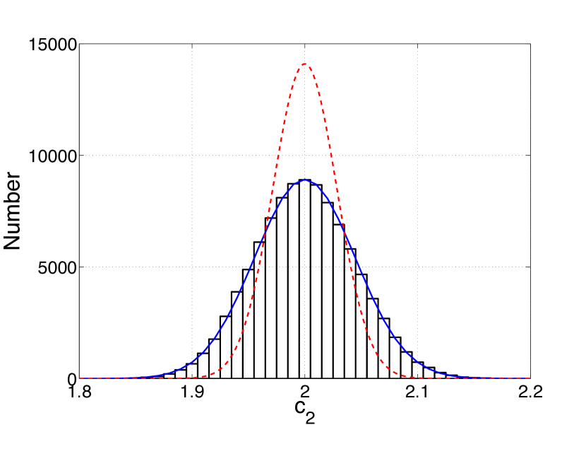
Figure 1: Histogram of the estimator for $c_{2}$ over $10^{5}$ realizations for the Laplace distribution and for a number of data point $T=10^{4}$. We assume here that the variance of the signal is 1 and the fourth cumulant is 3. The continuous line shows the non-Gaussian statistic density (a Gaussian centered around 2 with variance $\sigma_{U,NG}^{2}=c_{4}+2\alpha^{4}$ and the dashed line the Gaussian statistic density (a Gaussian centered in 2 with variance $\sigma_{U,G}^{2}=c_{4}$.

III Numerical Illustrations

III.1 Edgeworth expansions of usual distributions

Table 1: Test distributions used in this paper, their probability density and cumulants. Note that the $B_{j}$ are the so-called Bernoulli numbers ($B_{0}$=1, $B_{1}$=1/2, $B_{2}$=1/6, $B_{3}$=0, $B_{4}$=-1/30). The $K_{1}$ function is the Bessel function of the first kind.

PDF name	Probability density	Cumulants of order $j\left(c_{j}\right)$
Laplace	$\frac{a}{2}\exp\left(-a\left|x\right|\right)$	$c_{2j}=\frac{2\left(2j-1\right)!}{a^{2j}}$
Hypersecant	$\frac{1}{2a}\sec h\left(\frac{\pi}{2a}x\right)$	$c_{2j}=\left(-1\right)^{j+1}\left(2^{2j}-1\right)2^{2j-1}a^{2j}\frac{B_{2j}}{j}$
Logistic	$\frac{\exp\left(-\frac{x}{a}\right)}{a\left(1+\exp\left(-\frac{x}{a}\right)\right)^{2}}$	$c_{2j}=\left(-1\right)^{j-1}\frac{\left(2a\pi\right)^{2j}}{2j}B_{2j}$
NIG	$\frac{\delta a\exp\left(\delta a\right)}{\pi\sqrt{\delta^{2}+x^{2}}}K_{1}\left(a\sqrt{\delta^{2}+x^{2}}\right)$	$c_{2}=\frac{\delta}{a}$ ; $c_{4}=\frac{3\delta}{a^{3}}$

We now present a series of numerical illustrations showing how the methodology introduced in this paper can be applied to estimate not only the variance but also the fourth cumulant of the signal distribution. We first consider a list of 5 standard distributions, including the Gaussian distribution as well as 4 non-Gaussian distributions, namely the Laplace, hypersecant, logistic and normal inverse Gaussian distributions. These distributions are characterized in parametric form by their densities, with cumulants expressed as a function of the parameters of the density (see Table  1). The deviation from the Gaussian is measured in terms of the $c_{3}$ and $c_{4}$ parameters, which are zero for the Gaussian, and non-zero for non-Gaussian distributions. It should be noted that all distributions we analyze are symmetric, which implies that the parameter $c_{3}=0$. Beside, we choose the parameter values so that all distributions have a unit variance. More specifically, we make the following parametric choices.

1. Gaussian distribution, we take the parameter $a=1$, so that we have $c_{2}=1,$ $c_{3}=0$, $c_{4}=0$.

2. Laplace distribution, we take the parameter $a=1,$ so that we have $c_{2}=1,$ $c_{3}=0$, $c_{4}=12$.

3. Hypersecant distribution, we have that $c_{2}=a^{2},$ $c_{3}=0$ and $c_{4}=2a^{4}$; taking $a=1,$ we have that $c_{2}=1,$ $c_{3}=0$ and $c_{4}=2.$

4. Logistic distribution, we have that $c_{2}=\frac{a^{2}\pi^{2}}{3},$ $c_{3}=0$ and $c_{4}=\frac{2a^{4}\pi^{4}}{15}$; taking $a=\frac{\sqrt{3}}{\pi},$ we have that $c_{2}=1,$ $c_{3}=0$ and $c_{4}=18/15=1.2.$

5. Normal Inverse Gaussian distribution, we can take $a=$ $\delta=1$, so that we have $c_{2}=1,$ $c_{3}=0$, $c_{4}=3$.

For each non-Gaussian distribution in the table, we plot on the same graph for the chosen parameter values the exact density function of the signal $f_{s}\left(x\right)$ as well as the approximate density function, where the approximation is given the Edgeworth expansion $f_{s}^{E}\left(x\right)$. In addition to the quality of fit that can be visually assessed from the analysis of the graph, we also compute a quantitative measure of the approximation error AE as the quadratic distance between the exact and approximate density using the Edgeworth expansion:

$$AE^{E}=\left(\int\nolimits_{-\infty}^{+\infty}\left(f_{s}^{E}\left(x\right)-f_{s}\left(x\right)\right)^{2}dx\right)^{1/2}$$ (46)

For comparison purposes, we also report the approximation error with a simple Gaussian approximation, denoted by $AE^{G}$.

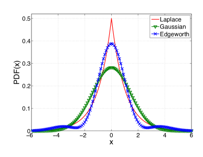
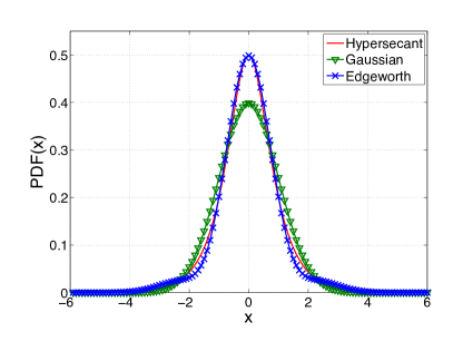
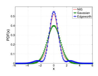
Figure 2: Edgeworth (crosses) and Gaussian (triangles) approximations for the Laplace (top left), Hypersecant (top right), Logistic (bottom left) and NIG (bottom right) distributions (continuous line). The approximation errors are respectively $AE^{E}=0.085$ and $AE^{G}=0.15$ (Laplace), $AE^{E}=0.03$ and $AE^{G}=0.085$ (Logistic), $AE^{E}=0.015$ and $AE^{G}=0.055$ (Hypersecant), $AE^{E}=0.0046$ and $AE^{G}=0.013$ (NIG). This gives an improvement of $\frac{AE^{G}}{AE^{E}}$ of 1.8 (Laplace), 2.8 (Logistic), 3.6 (Hypersecant) and 2.8 (NIG) .

The Edgeworth expansions appear to be a better fit compared to the Gaussian approximation for all non-Gaussian distributions that we consider, as can be seen from a simple visual inspection, and also more formally from the fact that approximation errors AE are from 2 to 4 times lower with the non-parametric expansions compared to what is obtained with the Gaussian approximation. The best fit is given by the NIG distribution with $\frac{AE^{G}}{AE^{E}}=1.8$ and the worse fit by the Laplace distribution with $\frac{AE^{G}}{AE^{E}}=3.6$.

III.2 Monte Carlo simulations and predictions

In order to test our new likelihood statistic, we generate fictitious data sets $h_{1}(t)$ and $h_{2}(t)$ at the output of two co-incident detectors, containing the GW signal $s(t)$, with an outcome randomly selected from the distributions presented above, and independent Gaussian noises $n_{1}(t)$ and $n_{2}(t)$. We then use the simulated data to obtain analytically the moment-based estimates for $c_{2}$ and $c_{4}$ and also to obtain numerically the maximum likelihood estimates for these parameters. The results for $c_{4}$ averaged over $10^{4}$ trials for a number of point $T=10^{6}$ and for the 4 distributions are presented in Table  2 and Figure  3. The number of points in a sample containing 1 year of data sampled at about 100 Hz will be rather of the order of $10^{9}$ but this would have required more computational resources than what we had available. In order to get a realistic estimate of the performance, one should therefore divide by $\sqrt{10^{3}}$ the standard deviations quoted in the table. The number of trials has an effect on the average estimated value, especially when the standard deviation is large. In the limit, we expect that using n increasing number of trials would generate an estimate that would converge to the injected value in all cases. For this reason we only considered values of the ratio $\alpha^{2}/\sigma_{n}^{2}$ larger than 0.03 (here we assume for simplicity that the variance of the noise is the same for both detectors, and we denote it by $\sigma_{1}=\sigma_{2}=\sigma_{n}$). With $\alpha^{2}/\sigma_{n}^{2}=0.01$, the uncertainty obtained with $10^{6}$ points is too large and we would need to average over more than $10^{4}$ trials to get a reasonably reliable estimate for$c_{4}$ . The results we obtain are very similar for the Logistic, Hypersecant and NIG distributions. The cumulant $c_{2}$ estimated with our new statistic, which we do not report here, is the same as the one derived analytically or obtained with the standard cross-correlation statistic, and is also in very good agreement with the injected value (better than 1% for 1 year). This suggests that our methodology allows us to estimate $c_{4}$ accurately without any negative impact on how well estimated is the $c_{2}$ parameter. Note that the ratio $\alpha^{2}/\sigma_{n}^{2}=0.01-0.1$ is in the range of predicted values for cosmological and astrophysical stochastic backgrounds for both Advanced LIGO and VIRGO detectors and Einstein Telescope. For cosmic strings, the typical value of the energy density parameter at 100 Hz is expected to be $\Omega_{gw}=10^{-9}-10^{-5}$ which corresponds to $\alpha^{2}/\sigma_{n}^{2}=10^{-6}-1$ for Advanced detectors and $\alpha^{2}/\sigma_{n}^{2}=10^{-4}-100$ for Einstein Telescope. For compact binary mergers, $\Omega_{gw}=10^{-10}-10^{-7}$ which corresponds to $\alpha^{2}/\sigma_{n}^{2}=10^{-7}-0.01$ for Advanced detectors and $\alpha^{2}/\sigma_{n}^{2}=10^{-5}-1$ for Einstein Telescope.

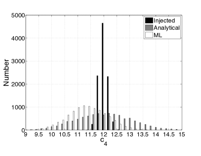
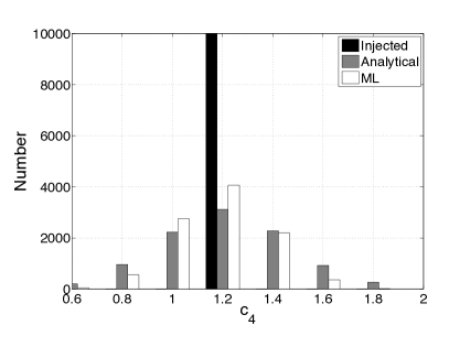
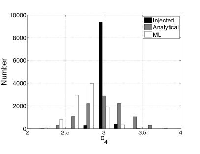
Figure 3: Histogram of $c_{4}$ injected (black), estimated analytically (grey) and estimated numerically by maximizing the likelihood function (white), for the distribution of Laplace (top left), Logistic (top right), hypersecant (bottom left) and NIG (bottom right). Each plot is the result of 10,000 realizations, each having $10^{6}$ points and with $\alpha^{2}/\sigma_{n}^{2}=0.1$.

Table 2: Average value over $10^{4}$ trials of $c_{4}$ estimated analytically and by likelihood maximization, for all the distributions considered in this paper, with standard deviation presented in parenthesis. The number of points in each trial is $10^{6}$. To obtain the estimation error for $10^{9}$ points, which corresponds to a sample of 1 year of data, one should divide the standard deviation by $\sqrt{(}10^{3})$.

Distribution		$\alpha^{2}\sigma_{n}^{-2}=0.03$	$\alpha^{2}\sigma_{n}^{-2}=0.05$	$\alpha^{2}\sigma_{n}^{-2}=0.1$
Laplace	anal	12.1 (9.6)	12.0 (3.7)	12.0 (1.1)
	ML	12.1 (6.1)	11.8 (2.4)	11.3 (0.7)
Hypersecant	anal	2.0 (2.0)	2.0 (0.9)	2.0 (0.3)
	ML	2.0 (1.4)	2.0 (0.6)	2.0 (0.2)
Logistic	anal	1.2 (2.4)	1.2 (0.9)	1.2 (0.3)
	ML	1.4 (1.3)	1.2 (0.6)	1.2 (0.2)
NIG	anal	3.0 (2.4)	3.0 (0.9)	3.0 (0.3)
	ML	3.0 (1.5)	3.0 (0.6)	2.9 (0.2)

We find that the fourth cumulant parameter is estimated with reasonably good precision for the cases under investigation. We also find that the maximum likelihood estimator generates an estimation error lower than that of the moment-based estimator, which is consistent with the general statement that the maximum likelihood estimator is asymptotically efficient.

IV Extending the Approach to the Detection of Signals in the Popcorn Regime

A gravitational wave stochastic background is produced by a collection of independent gravitational wave events. In some cases, the ratio of the average time between events to the average duration of an event is small and a large number of events are taking place simultaneously. In other cases, the ratio is large and the signal received has a popcorn signature. In what has been discussed so far in this paper, we have analyzed the first type of situations, and implicitly considered that GW events were too numerous to be individually distinguished, and yet not numerous enough for central limit theorem to give a strictly Gaussian distribution, with a deviation explicitly characterized in terms of the Edgeworth expansion. We now turn to an analysis of the second type of situations, following and generalizing an approach introduced by DF03 Drasco and Flanagan (2003), who have focused on a model where the deviation from the Gaussian distributional assumption was understood as emanating from the presence of a resolved Gaussian signal being measured with a probability $0<\xi\leq 1$ (the Gaussian case is recovered for $\xi=1$). In DF03 Drasco and Flanagan (2003), the observed distribution was assumed to the of the following form:

$$f_{s}\left(s_{t}\right)=\xi f_{G}\left(s_{t}\right)+\left(1-\xi\right)\delta\left(s_{t}\right)=\xi\frac{1}{\sqrt{2\pi}\alpha}e^{-\frac{s_{t}^{2}}{2\alpha^{2}}}+\left(1-\xi\right)\delta\left(s_{t}\right)$$ (47)

where the parameter $0<\xi\leq 1$ and $\delta\left(.\right)$ is the density of the Dirac distribution. Since by assumption the events that are measured are supposed to be in small numbers, the Gaussian assumption is hard to justify and should be relaxed. We generalize this model by considering:

$$f_{s}\left(s_{t}\right)=\xi f_{NG}\left(s_{t}\right)+\left(1-\xi\right)\delta\left(s_{t}\right)$$ (48)

and we further assume that the unknown non-Gaussian density $f_{NG}$ can be approximated by a 4th order Edgeworth expansion

$$f_{s}\left(s_{t}\right) = \xi f_{G}\left(s_{t}\right)g\left(s_{t}\right)+\left(1-\xi\right)\delta\left(s_{t}\right)$$ (49)

$$= \xi\frac{1}{\sqrt{2\pi}\alpha}e^{-\frac{s_{t}^{2}}{2\alpha^{2}}}\left[1+\frac{c_{3}}{6\alpha^{3}}H_{3}\left(\frac{x}{\alpha}\right)+\frac{c_{4}}{24\alpha^{4}}H_{4}\left(\frac{x}{\alpha}\right)+\frac{c_{3}^{2}}{72\alpha^{6}}H_{6}\left(\frac{x}{\alpha}\right)\right]+\left(1-\xi\right)\delta\left(s_{t}\right)$$ (50)

Using this expression for the signal density, we obtain the following generalized form for the likelihood ratio:

$$\Lambda_{ML} = \frac{\underset{\alpha,c_{3},c_{4},\sigma_{1},\sigma_{2},\xi}{\max}\int f_{s}\left(s\right)f_{n}\left(h-s\right)ds}{\underset{\sigma_{1},\sigma_{2}}{\max}f_{n}}$$

$$= \underset{\alpha,c_{3},c_{4},\sigma_{1},\sigma_{2},\xi}{\max}\prod\limits_{t=1}^{T}\frac{\overline{\sigma}_{1}\overline{\sigma}_{2}}{\sigma_{1}\sigma_{2}}\int_{-\infty}^{+\infty}f_{s}\left(s_{t}\right)\exp\left[-\frac{\left(h_{1t}-s_{t}\right)^{2}}{2\sigma_{1}^{2}}-\frac{\left(h_{2t}-s_{t}\right)^{2}}{2\sigma_{2}^{2}}+1\right]ds_{t}$$

$$= \underset{\alpha,c_{3},c_{4},\sigma_{1},\sigma_{2},\xi}{\max}\prod\limits_{t=1}^{T}\frac{\overline{\sigma}_{1}\overline{\sigma}_{2}}{\sigma_{1}\sigma_{2}}\int_{-\infty}^{+\infty}\left[\xi f_{G}\left(s_{t}\right)g\left(s_{t}\right)+\left(1-\xi\right)\delta\left(s_{t}\right)\right]\exp\left[-\frac{\left(h_{1t}-s_{t}\right)^{2}}{2\sigma_{1}^{2}}-\frac{\left(h_{2t}-s_{t}\right)^{2}}{2\sigma_{2}^{2}}+1\right]ds_{t}$$

After calculations similar to what has been done before for the case with $\xi=1$ , we obtain:

$$\Lambda_{ML} = \underset{\alpha,c_{3},c_{4},\sigma_{1},\sigma_{2},\xi}{\max}\prod\limits_{t=1}^{T}\left\{\xi\frac{\sigma}{\alpha}\frac{\overline{\sigma}_{1}\overline{\sigma}_{2}}{\sigma_{1}\sigma_{2}}\exp\left[-\frac{h_{1t}^{2}}{2\sigma_{1}^{2}}-\frac{h_{2t}^{2}}{2\sigma_{2}^{2}}+1\right]\exp\left[\frac{1}{2}\sigma^{2}\left(\frac{h_{1t}}{\sigma_{1}^{2}}+\frac{h_{2t}}{\sigma_{2}^{2}}\right)^{2}\right]\right.$$

$$\left.\times\left(I_{0}+I_{1t}+I_{2t}+I_{3t}+I_{4t}+I_{6t}\right)+\left(1-\xi\right)\frac{\overline{\sigma}_{1}\overline{\sigma}_{2}}{\sigma_{1}\sigma_{2}}\exp\left[-\frac{h_{1t}^{2}}{2\sigma_{1}^{2}}-\frac{h_{2t}^{2}}{2\sigma_{2}^{2}}+1\right]\right\}$$

The values of $1-\xi,$ $\alpha,$ $c_{3},$ $c_{4},$ $\sigma_{1},$ $\sigma_{2},$ that achieve the maximum value for the likelihood function are, respectively, estimators for the probability of the presence of a (non-Gaussian) signal, the 2nd, 3rd and 4th cumulant of the signal distirbutions, and the variance of the noise in the two detectors. Note that if we evaluate this function at $\xi=1$, $c_{3}=c_{4}=0$, rather than maximizing over $\xi,$ $c_{3}$, $c_{4}$, we recover the Gaussian detection statistic.

V Conclusions and Directions for Further Research

This paper introduces a non-parametric approach to the detection of non-Gaussian gravitational wave stochastic backgrounds. The approach we propose is based on Edgeworth expansion, which is a formal expansion of the characteristic function of the signal distribution, whose unknown probability density function is to be approximated in terms of the characteristic function of the Gaussian distribution. The non-Gaussian detection statistic we obtain generalizes the standard cross-correlation statistic that is recovered in the limit of vanishing third and fourth cumulants of the empirical conditional distribution of the detector measurement. Our paper complements related work by DF03 Drasco and Flanagan (2003), who have focused on a very specific model where the deviation from the Gaussian distributional assumption was understood as emanating from the presence of a resolved Gaussian signal being measured. We provide a methodology that can be applied without any assumption regarding the exact nature of the departure from normality, and which relies on an explicit correction to the central limit theorem, when the number of sources is finite. The main benefit of the procedure is that it allows us to estimate additional parameters when the signal is not too small compared to the noise ($\alpha^{2}/\sigma_{n}^{2}$ of the order of 0.01), namely the 3rd and 4th cumulant of the gravitational wave signal distribution, which should be useful for analyzing the constraints on astrophysical and cosmological models that will be imposed by observed gravitation wave signals, and comparing them to the constraints derived from supernovae or galaxy clusters observations. Our methodology can be extended to a situation when there is uncertainty about the signal presence, e.g., in the case of bursts, where there is a positive probability of having no signal, and having few of them simultaneously when they are there, which would allow us to generalize the methodology in DF03 Drasco and Flanagan (2003) to a non-Gaussian signal.

More generally, we may also account for the presence of a random, exponentially-distributed, number of sources, each of which having a non-Gaussian distribution, by using formal expansions for compound Poisson processes (see for example Babu et al. (2003)). Our approach is also flexible enough to be extended to the presence of non-Gaussian noise distributions, in addition to the presence of non-Gaussian signal distribution. This extension would be useful since significant non-Gaussian tails have been obtained for the noise distributions of all gravitational waves detectors (see Allen et al. (2003)) and will be the purpose of a future paper.

Finally, in this paper we considered coincident detectors. This assumption is valid for Einstein Telescope but more work is needed to extend our results to a network of separated detectors such as LIGO/Virgo network.

References

- Grishchuk (1975) L. P. Grishchuk, Soviet Journal of Experimental and Theoretical Physics 40, 409 (1975).
- Grishchuk (1993) L. P. Grishchuk, Phys. Rev. D 48, 3513 (1993), eprint gr-qc/9304018.
- Starobinskiǐ (1979) A. A. Starobinskiǐ, Soviet Journal of Experimental and Theoretical Physics Letters 30, 682 (1979).
- Gasperini and Veneziano (1993) M. Gasperini and G. Veneziano, Astroparticle Physics 1, 317 (1993), eprint hep-th/9211021.
- Buonanno et al. (1997) A. Buonanno, M. Maggiore, and C. Ungarelli, Phys. Rev. D 55, 3330 (1997), eprint gr-qc/9605072.
- Dufaux et al. (2010) J.-F. Dufaux, D. G. Figueroa, and J. García-Bellido, Phys. Rev. D 82, 083518 (2010), eprint 1006.0217.
- Damour and Vilenkin (2005) T. Damour and A. Vilenkin, Phys. Rev. D 71, 063510 (2005), eprint hep-th/0410222.
- Siemens et al. (2007) X. Siemens, V. Mandic, and J. Creighton, Physical Review Letters 98, 111101 (2007), eprint astro-ph/0610920.
- Ölmez et al. (2010) S. Ölmez, V. Mandic, and X. Siemens, Phys. Rev. D 81, 104028 (2010), eprint 1004.0890.
- Regimbau et al. (2012) T. Regimbau, S. Giampanis, X. Siemens, and V. Mandic, Phys. Rev. D 85, 066001 (2012), eprint 1111.6638.
- Caprini et al. (2008) C. Caprini, R. Durrer, and G. Servant, Phys. Rev. D 77, 124015 (2008), eprint 0711.2593.
- Caprini et al. (2009a) C. Caprini, R. Durrer, T. Konstandin, and G. Servant, Phys. Rev. D 79, 083519 (2009a), eprint 0901.1661.
- Caprini et al. (2009b) C. Caprini, R. Durrer, and G. Servant, Journal of Cosmology and Astroparticle Physics 12, 024 (2009b), eprint 0909.0622.
- Maggiore (2000) M. Maggiore, Physics Reports 331, 283 (2000), eprint gr-qc/9909001.
- Binétruy et al. (2012) P. Binétruy, A. Bohé, C. Caprini, and J.-F. Dufaux, Journal of Cosmology and Astroparticle Physics 6, 027 (2012), eprint 1201.0983.
- Regimbau (2011) T. Regimbau, Research in Astronomy and Astrophysics 11, 369 (2011), eprint 1101.2762.
- Buonanno et al. (2005) A. Buonanno, G. Sigl, G. G. Raffelt, H.-T. Janka, and E. Müller, Phys. Rev. D 72, 084001 (2005), eprint astro-ph/0412277.
- Sandick et al. (2006) P. Sandick, K. A. Olive, F. Daigne, and E. Vangioni, Phys. Rev. D 73, 104024 (2006), eprint astro-ph/0603544.
- Marassi et al. (2009) S. Marassi, R. Schneider, and V. Ferrari, Monthly Notices of the Royal astronomical Society 398, 293 (2009), eprint 0906.0461.
- Zhu et al. (2010) X.-J. Zhu, E. Howell, and D. Blair, Monthly Notices of the Royal astronomical Society 409, L132 (2010), eprint 1008.0472.
- Regimbau and de Freitas Pacheco (2001) T. Regimbau and J. A. de Freitas Pacheco, Astronomy and Astrophysics 376, 381 (2001), eprint astro-ph/0105260.
- Rosado (2012) P. A. Rosado, Phys. Rev. D 86, 104007 (2012), eprint 1206.1330.
- Regimbau and de Freitas Pacheco (2006) T. Regimbau and J. A. de Freitas Pacheco, Astronomy and Astrophysics 447, 1 (2006), eprint astro-ph/0509880.
- Howell et al. (2011) E. Howell, T. Regimbau, A. Corsi, D. Coward, and R. Burman, Monthly Notices of the Royal astronomical Society 410, 2123 (2011), eprint 1008.3941.
- Marassi et al. (2011a) S. Marassi, R. Ciolfi, R. Schneider, L. Stella, and V. Ferrari, Monthly Notices of the Royal astronomical Society 411, 2549 (2011a), eprint 1009.1240.
- Wu et al. (2013) C.-J. Wu, V. Mandic, and T. Regimbau, Phys. Rev. D 87, 042002 (2013).
- de Araujo and Marranghello (2009) J. C. N. de Araujo and G. F. Marranghello, General Relativity and Gravitation 41, 1389 (2009), eprint 0910.0424.
- Ferrari et al. (1999) V. Ferrari, S. Matarrese, and R. Schneider, Monthly Notices of the Royal astronomical Society 303, 258 (1999), eprint astro-ph/9806357.
- Zhu et al. (2011a) X.-J. Zhu, X.-L. Fan, and Z.-H. Zhu, Astrophys. J. 729, 59 (2011a), eprint 1102.2786.
- Howell et al. (2004) E. Howell, D. Coward, R. Burman, D. Blair, and J. Gilmore, Monthly Notices of the Royal astronomical Society 351, 1237 (2004).
- Zhu et al. (2011b) X.-J. Zhu, E. Howell, T. Regimbau, D. Blair, and Z.-H. Zhu, Astrophys. J. 739, 86 (2011b), eprint 1104.3565.
- Rosado (2011) P. A. Rosado, Phys. Rev. D 84, 084004 (2011), eprint 1106.5795.
- Marassi et al. (2011b) S. Marassi, R. Schneider, G. Corvino, V. Ferrari, and S. P. Zwart, Phys. Rev. D 84, 124037 (2011b), eprint 1111.6125.
- Wu et al. (2012) C. Wu, V. Mandic, and T. Regimbau, Phys. Rev. D 85, 104024 (2012), eprint 1112.1898.
- Zhu et al. (2013) X.-J. Zhu, E. J. Howell, D. G. Blair, and Z.-H. Zhu, Monthly Notices of the Royal astronomical Society 431, 882 (2013), eprint 1209.0595.
- the Advanced LIGO Team (2007) the Advanced LIGO Team (2007), URL https://dcc.ligo.org/cgi-bin/DocDB/ShowDocument?docid=m060056.
- Losurdo and the Advanced Virgo Team (2007) G. Losurdo and the Advanced Virgo Team (2007), URL https://tds.ego-gw.it/ql/?c=1900.
- Punturo et al. (2010) M. Punturo et al., Classical and Quantum Gravity 27, 194002 (2010), URL http://stacks.iop.org/0264-9381/27/i=19/a=194002.
- Allen and Romano (1999) B. Allen and J. D. Romano, Phys. Rev. D 59, 102001 (1999), eprint gr-qc/9710117.
- Coward and Burman (2005) D. M. Coward and R. R. Burman, Monthly Notices of the Royal Astronomical Society 361, 362 (2005), eprint astro-ph/0505181.
- Drasco and Flanagan (2003) S. Drasco and É. É. Flanagan, Phys. Rev. D 67, 082003 (2003), eprint gr-qc/0210032.
- Seto (2009) N. Seto, Phys. Rev. D 80, 043003 (2009), eprint 0908.0228.
- Thrane (2013) E. Thrane, Phys. Rev. D 87, 043009 (2013), eprint 1301.0263.
- Feller (2008) W. Feller, An introduction to probability theory and its applications (John Wiley & Sons, 2008).
- Gallant and Nychka (1987) A. R. Gallant and D. W. Nychka, Econometrica: Journal of the Econometric Society pp. 363–390 (1987).
- Gallant and Tauchen (1989) A. R. Gallant and G. Tauchen, Econometrica: Journal of the Econometric Society pp. 1091–1120 (1989).
- Box et al. (1978) G. E. Box, W. G. Hunter, and J. S. Hunter (1978).
- Omey and Van Gulck (2008) E. Omey and S. Van Gulck (2008).
- Babu et al. (2003) G. J. Babu, K. Singh, and Y. Yang, Annals of the Institute of Statistical Mathematics 55, 83 (2003).
- Allen et al. (2003) B. Allen, J. D. E. Creighton, É. É. Flanagan, and J. D. Romano, Phys. Rev. D 67, 122002 (2003), eprint gr-qc/0205015.