Evolution equation for geometric quantum correlation measures

Abstract

A simple relation is established for the evolution equation of quantum information processing protocols such as quantum teleportation, remote state preparation, Bell-inequality violation and particularly dynamics of the geometric quantum correlation measures. This relation shows that when the system traverses the local quantum channel, various figures of merit of the quantum correlations for different protocols demonstrate a factorization decay behavior for dynamics. We identified the family of quantum states for different kinds of quantum channels under the action of which the relation holds. This relation simplifies the assessment of many quantum tasks.

I Introduction

Quantum theory enables the processing of quantum information with efficiency that outperforms the classical information processing. The quantum correlations, quantified by various measures, of the computational systems were considered to be the origin of this superiority RMP1 . But when implementing the quantum information processing (QIP) tasks experimentally, one has to face the unavoidable interaction of the quantum devices with their environments, the process of which often induces decay of correlations because of decoherence open . The lost of quantum correlation can generally damage the superiority of QIP. Therefore, it is of practical significance to make clear the behavior of a correlation when it serves as a resource in carrying out certain QIP tasks. The process of the decoherence effects can be in general described as the time evolution of the quantum system.

To assess the time evolution of a given quantum correlation measure, one usually needs to derive first the time-dependence of the density matrix, and this is intractable. From a theoretical point of view, one needs to obtain the evolution of the system for every initial states, while from an experimental point of view, it requires the full reconstruction of the evolved state via quantum tomography tomography . This either needs much computational resources or is hard to do experimentally.

Seeking general dynamical law for various correlation measures can simplify these tasks. As an earlier proposed scenario of quantum correlation measure, entanglement has been the focus of researchers for years RMP1 . Particularly, when one party of a two-qubit system traverses a noisy channel, the evolution equation of concurrence con was found to be governed by a factorization law for the initial pure states natphys . This simplifies the assessment of the evolution of concurrence as to evaluate a decay factor. Soon a universal curve describing the evolution of concurrence for general two-qubit states was revealed science . Since then, the evolution equations for many other entanglement measures FL1 ; FL2 ; FL3 or their bounds FLb1 ; FLb2 ; FLb3 were derived.

Besides entanglement, the quantumness of correlations can also be characterized from other perspectives. Those measures are such as the conventional quantum discord qd , geometric quantum discord (GQD) gqd ; gqd1 ; trace ; trace1 ; lqu ; square , and measurement-induced nonlocality min ; min1 , which are also resources for certain QIP tasks appl ; Dakic ; Guml . Moreover, many measures related to the explicit quantum tasks (see the following text) reveal also some kinds of correlations. The decay dynamics for them under different environments have been extensively studied Modirmp ; dyn0 ; dyn1 ; dyn2 ; dyn3 ; dyn4 ; dyn5 . Yet, some general conclusions still remain absent. Motivated by these, we study in this paper the evolution equations for various geometric correlation measures when the system traverses a local quantum channel. We will show that for a broad class of quantum states, the evolution equations of the considered correlations are fully characterized by the product of the initial correlation and a time-dependent factor determined solely by the structure of the channel. This facilitates greatly the estimation of the robustness of the correlations in realistic physical systems.

II Preliminaries

Consider a general bipartite state $\rho$ in the Hilbert space $\mathcal{H}_{ab}$. It can always be decomposed as

$$\rho=-\frac{1}{d_{a}d_{b}}\mathbb{I}_{a}\otimes\mathbb{I}_{b}+\rho_{a}\otimes\frac{1}{d_{b}}\mathbb{I}_{b}+\frac{1}{d_{a}}\mathbb{I}_{a}\otimes\rho_{b}+\rho_{c},$$ (1)

where the reduced states $\rho_{a}={\rm tr}_{b}\rho$, $\rho_{b}={\rm tr}_{a}\rho$, and the traceless `correlation operator' $\rho_{c}$ are give by

$$\begin{split}&\rho_{a}=\frac{1}{d_{a}}\mathbb{I}_{a}+\vec{x}\cdot\vec{X},~{}\rho_{b}=\frac{1}{d_{b}}\mathbb{I}_{b}+\vec{y}\cdot\vec{Y},\\ &\rho_{c}=\sum_{i=1}^{d_{a}^{2}-1}\sum_{j=1}^{d_{b}^{2}-1}t_{ij}X_{i}\otimes Y_{j},\end{split}$$ (2)

with $\vec{x}=(x_{1},x_{2},\ldots,x_{d_{a}^{2}-1})^{t}$, $\vec{X}=(X_{1},X_{2},\ldots,X_{d_{a}^{2}-1})^{t}$ ($d_{a}={\rm dim}\mathcal{H}_{a}$, and $t$ denotes transpose), and likewise for $\vec{y}$ and $\vec{Y}$. $\{\mathbb{I}_{a}/\sqrt{d_{a}},\vec{X}\}$ and $\{\mathbb{I}_{b}/\sqrt{d_{b}},\vec{Y}\}$ constitute the orthonormal operator bases for $\mathcal{H}_{a}$ and $\mathcal{H}_{b}$, respectively.

Two extensively studied cases in the literature are $d_{a,b}=2$ and $3$, for which $X_{i}$ (and $Y_{j}$) are given respectively by $\sigma_{i}/\sqrt{2}~{}$ ($i=1,2,3$) and $\lambda_{j}/\sqrt{2}~{}$ ($j=1,2,\ldots,8$), with $\sigma_{i}$ and $\lambda_{j}$ being the Pauli and the Gell-Mann matrices. They can describe the qubit, the qutrit, and the hybrid qubit-qutrit systems, which are of central relevance to QIP.

The decomposed $\rho$ in Eq. (1) enables the definition of correlation measures from a geometric perspective. We consider here the definition of the general form

$$D_{p}(\rho)=\mathop{\rm opt}_{\Pi^{a}\in\mathcal{M}}\parallel\rho-\Pi^{a}(\rho)\parallel_{p}^{p},$$ (3)

where $\parallel\chi\parallel_{p}=[\mbox{tr}(\chi^{\dagger}\chi)^{p/2}]^{1/p}$ is the Schatten $p$-norm, and opt represents the optimization over some class $\mathcal{M}$ of the local measurements $\Pi^{a}=\{\Pi_{k}^{a}\}$ acting on party $a$.

Eq. (3) covers a series of discord-like correlation measures being proposed recently. (i) If opt represents minimum and $\mathcal{M}$ is that of the projective measurements, one recovers the 2-norm GQD for $p=2$ gqd , and the 1-norm GQD for $p=1$ trace . (ii) If $\rho$ is replaced by $\sqrt{\rho}$, then one obtains the Hellinger distance quantum discord for $p=2$ lqu ; square . (iii) If opt represents maximum and $\mathcal{M}$ is confined to the locally invariant measurements that maintain $\rho_{a}$, Eq. (3) turns to be the conventional measurement-induced nonlocality for $p=2$ min , and its modified version for $p=1$ min1 .

Besides $D_{p}(\rho)$ that is determined by $\vec{x}$, $\vec{y}$, and the matrix $T=(t_{ij})$, there are other measures related to explicit quantum protocols that are determined solely by $T$. We consider here the protocols of quantum teleportation, remote state preparation, and Bell-inequality violation. It has been shown that the average fidelity of quantum teleportation fide , remote state preparation Dakic , and the maximum Bell-inequality violation Bell were given respectively by

$$\begin{split}&\mathcal{F}_{\rm qt}(\rho)=\frac{1}{2}+\frac{1}{6}\mathcal{N}_{\rm qt}(\rho),~{}\mathcal{F}_{\rm rsp}(\rho)=\frac{1}{2}(E_{2}+E_{3}),\\ &\mathcal{B}_{\rm max}(\rho)=2\sqrt{E_{1}+E_{2}},\end{split}$$ (4)

where $\mathcal{N}_{\rm qt}(\rho)={\rm tr}\sqrt{T^{\dagger}T}$, and $E_{1}\geq E_{2}\geq E_{3}$ are the eigenvalues of $T^{\dagger}T$.

III General results

We restrict ourselves in the following to the projective measurements $\Pi^{a}$, then it follows from Eqs. (1) and (3) that $D_{p}(\rho)$ is solely determined by $\vec{x}$ and $T$, i.e.,

$$D_{p}(\rho)=\mathop{\rm opt}_{\Pi^{a}\in\mathcal{M}}\parallel\varrho-\Pi^{a}(\varrho)\parallel_{p}^{p},$$ (5)

where

$$\varrho=\vec{x}\cdot\vec{X}\otimes\frac{1}{d_{b}}\mathbb{I}_{b}+\rho_{c}.$$ (6)

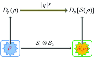
Figure 1: (Color online) Comparison of state evolution and geometric correlation dynamics. For certain family of $\rho$ (denoted by the color shaded region) the evolution equation for $D_{p}[\mathcal{S}(\rho)]$ can be deduced from $D_{p}(\rho)$.

Now, we suppose the considered system $ab$ passes through a quantum channel $\mathcal{S}$ such that

$$\vec{x}^{\prime}=q(t)\vec{x},~{}T^{\prime}=q(t)T,$$ (7)

with $q(t)$ being a time-dependent factor that contains only the information on the channel's structure, and the primed parameters $\vec{x}^{\prime}$ and $T^{\prime}$ denote respectively the local Bloch vector and the correlation tensor for $\mathcal{S}(\rho)$, similar as those for $\rho$ in Eq. (2). Then, from Eq. (7) we know that $\varrho^{\prime}=q(t)\varrho$, and therefore, as illustrated in Fig. 1, the formula of Eq. (5) implies that the evolution equation of $D_{p}[\mathcal{S}(\rho)]$ fulfills the following factorization decay behavior

$$D_{p}[\mathcal{S}(\rho)]=|q(t)|^{p}D_{p}(\rho),$$ (8)

which is solely determined by the product of the initial $D_{p}(\rho)$ and a channel-dependent factor $|q(t)|$.

In the operator-sum representation, the evolved state of the system $ab$ under the action of the local quantum channel $\mathcal{S}_{1}\otimes\mathcal{S}_{2}$ (it reduces to the one-sided channel when $\mathcal{S}_{1}=\mathbb{I}_{a}$ or $\mathcal{S}_{2}=\mathbb{I}_{b}$) can be written compactly as

$$(\mathcal{S}_{1}\otimes\mathcal{S}_{2})\rho=\sum_{\mu\nu}E_{\mu\nu}\rho E_{\mu\nu}^{\dagger},$$ (9)

where $\mathcal{S}_{1}$ denotes the channel for subsystem $a$ and $\mathcal{S}_{2}$ for subsystem $b$, and the Kraus operators $E_{\mu\nu}=E_{\mu}\otimes E_{\nu}$, with $E_{\mu}$ and $E_{\nu}$ satisfy $\sum_{\mu}E_{\mu}^{\dagger}E_{\mu}=\mathbb{I}_{a}$ and $\sum_{\nu}E_{\nu}^{\dagger}E_{\nu}=\mathbb{I}_{b}$.

In order to obtain the conditions under which the evolution equations of $D_{p}[\mathcal{S}(\rho)]$ obeying the relation (8), we turn to the Heisenberg picture. Then as $x_{i}={\rm tr}\rho(X_{i}\otimes\mathbb{I}_{b})$, $y_{j}={\rm tr}\rho(\mathbb{I}_{a}\otimes Y_{j})$, and $t_{ij}={\rm tr}\rho(X_{i}\otimes Y_{j})$ from Eq. (1), we obtain

$$x_{i}^{\prime}={\rm tr}[\rho\mathcal{S}_{1}^{\dagger}(X_{i})\otimes\mathbb{I}_{b}],~{}y_{j}^{\prime}={\rm tr}[\rho\mathbb{I}_{a}\otimes\mathcal{S}_{2}^{\dagger}(Y_{j})],$$ (10)

and

$$\begin{split}t_{ij}^{\prime}&={\rm tr}[(\mathcal{S}_{1}\otimes\mathcal{S}_{2})\rho(X_{i}\otimes Y_{j})]\\ &=\sum_{\mu\nu}{\rm tr}[E_{\mu\nu}\rho E_{\mu\nu}^{\dagger}(X_{i}\otimes Y_{j})]\\ &=\sum_{\mu\nu}{\rm tr}[\rho E_{\mu\nu}^{\dagger}(X_{i}\otimes Y_{j})E_{\mu\nu}]\\ &={\rm tr}[\rho\mathcal{S}_{1}^{\dagger}(X_{i})\otimes\mathcal{S}_{2}^{\dagger}(Y_{j})],\end{split}$$ (11)

where $\mathcal{S}_{1}^{\dagger}(X_{i})=\sum_{\mu}E_{\mu}^{\dagger}X_{i}E_{\mu}$ denotes the map of $\mathcal{S}_{1}$ on $X_{i}$, and likewise for $\mathcal{S}_{2}^{\dagger}(Y_{j})$. We have also used the facts $\mathcal{S}_{1}^{\dagger}(\mathbb{I}_{a})=\mathbb{I}_{a}$ and $\mathcal{S}_{2}^{\dagger}(\mathbb{I}_{b})=\mathbb{I}_{b}$ when deriving Eq. (10).

Then, from the above two equations one can derive that Eq. (7) can be satisfied by a broad class of quantum channels, for which we will discuss in the framework of the one-sided cases $\mathcal{S}_{1}\otimes\mathbb{I}_{b}$ and $\mathbb{I}_{a}\otimes\mathcal{S}_{2}$, and the two-sided case $\mathcal{S}_{1}\otimes\mathcal{S}_{2}$.

Theorem 1. If a channel gives $\mathcal{S}_{1}^{\dagger}(X_{i})=q_{a}X_{i}$ for all $\{X_{i}\}$, and $\mathcal{S}_{2}^{\dagger}(Y_{j})=q_{b}Y_{j}$ for all $\{Y_{j}\}$, then $D_{p}[\mathcal{S}(\rho)]$ obeys the factorization decay behavior of Eq. (8) for the families of $\rho$ with

$$(1) ~{}\mbox{arbitrary}~{}\rho_{a},~{}\rho_{b},~{}\rho_{c}~{}~{}(\mbox{for \,}\mathcal{S}_{1}\otimes\mathbb{I}_{b}),$$ (12)

$$(2) ~{}\rho_{a}=\frac{1}{d_{a}}\mathbb{I}_{a},\mbox{or~{}}\rho_{c}=0~{}~{}(\mbox{for \,}\mathcal{S}_{1}\otimes\mathcal{S}_{2}~{}\mbox{with~{}}\mathcal{S}_{2}\neq\mathbb{I}_{b}).$$

Proof. As for $\mathcal{S}_{1}\otimes\mathcal{S}_{2}$, we have $\vec{x}^{\prime}=q_{a}\vec{x}$ and $T^{\prime}=q_{a}q_{b}T$. Then it is direct to see that for the special case $\mathcal{S}_{2}=\mathbb{I}_{b}$ which corresponds to $q_{b}=1$, Eq. (7) is always satisfied, and thus the factorization decay behavior of Eq. (8) holds for arbitrary bipartite state $\rho$, i.e., there is no restriction on $\rho_{a}$, $\rho_{b}$, and $\rho_{c}$. For $\mathcal{S}_{1}\otimes\mathcal{S}_{2}$ with $\mathcal{S}_{2}\neq\mathbb{I}_{b}$, however, Eq. (7) is satisfied only when $\vec{x}=0$ or $T=0$, which corresponds to the family of $\rho$ with $\rho_{a}=\mathbb{I}_{a}/{d_{a}}$ or $\rho_{c}=0$. This completes the proof. $\blacksquare$

In general, $\mathcal{S}_{1}\otimes\mathcal{S}_{2}$ includes the channels $\mathcal{S}_{1}\otimes\mathbb{I}_{b}$ and $\mathbb{I}_{a}\otimes\mathcal{S}_{2}$ as two special cases, and thus the range of states for $\mathcal{S}_{1}\otimes\mathbb{I}_{b}$ and $\mathbb{I}_{a}\otimes\mathcal{S}_{2}$ should be at least as large as that for $\mathcal{S}_{1}\otimes\mathcal{S}_{2}$. This is indeed what Theorem 1 implies, as there is no restriction on the range of states for family (1), while family (2) includes only those $\rho$ with $\rho_{a}=\mathbb{I}_{a}/{d_{a}}$ or $\rho_{c}=0$.

Theorem 2. If $\mathcal{S}_{1}^{\dagger}(X_{k})=q_{a}X_{k}$ only for $\{X_{k}\}$ with $k=\{k_{1},\ldots,k_{\alpha}\}$ ($\alpha<d_{a}^{2}-1$), and $\mathcal{S}_{2}^{\dagger}(Y_{l})=q_{b}Y_{l}$ only for $\{Y_{l}\}$ with $l=\{l_{1},\ldots,l_{\beta}\}$ ($\beta<d_{b}^{2}-1$), then $D_{p}[\mathcal{S}(\rho)]$ obeys the factorization decay behavior of Eq. (8) for the families of $\rho$ with

$$(1) ~{}\rho_{a}=\rho_{a}^{(1)},~{}\rho_{c}=\rho_{c}^{(1)}~{}~{}(\mbox{for \,}\mathcal{S}_{1}\otimes\mathbb{I}_{b}),$$ (13)

$$(2) ~{}\rho_{a}=\frac{1}{d_{a}}\mathbb{I}_{a},~{}\rho_{c}=\rho_{c}^{(2)},~{}\mbox{or~{}}\rho_{c}=0~{}(\mbox{for \,}\mathbb{I}_{a}\otimes\mathcal{S}_{2}),$$

$$(3) ~{}\rho_{a}=\frac{1}{d_{a}}\mathbb{I}_{a},~{}\rho_{c}=\rho_{c}^{(3)},~{}\mbox{or~{}}\rho_{a}=\rho_{a}^{(1)},~{}\rho_{c}=0$$

$$~{}(\mbox{for \,}\mathcal{S}_{1}\otimes\mathcal{S}_{2}),$$

where

$$\begin{split}&\rho_{a}^{(1)}=\frac{1}{d_{a}}\mathbb{I}_{a}+\sum_{k=k_{1}}^{k_{\alpha}}x_{k}X_{k},~{}\rho_{c}^{(1)}=\sum_{k=k_{1}}^{k_{\alpha}}\sum_{j=1}^{d_{b}^{2}-1}t_{kj}X_{k}\otimes Y_{j},\\ &\rho_{c}^{(2)}=\sum_{i=1}^{d_{a}^{2}-1}\sum_{l=l_{1}}^{l_{\beta}}t_{il}X_{i}\otimes Y_{l},~{}\rho_{c}^{(3)}=\sum_{k=k_{1}}^{k_{\alpha}}\sum_{l=l_{1}}^{l_{\beta}}t_{kl}X_{k}\otimes Y_{l}.\end{split}$$ (14)

Proof. As $\mathcal{S}_{1}^{\dagger}(X_{k})=q_{a}X_{k}$ and $\mathcal{S}_{2}^{\dagger}(Y_{l})=q_{b}Y_{l}$ only for partial $\{X_{k}\}$ and $\{Y_{l}\}$, then if components of the local Bloch vector and the correlation tensor, namely, those $x_{i}$ and $t_{ij}$ related to $\mathcal{S}_{1}^{\dagger}(X_{i})\neq q_{a}X_{i}$ or/and $\mathcal{S}_{2}^{\dagger}(Y_{j})\neq q_{b}Y_{j}$ equal zero, the requirement in Eq. (7) is always satisfied for $\mathcal{S}_{1}\otimes\mathbb{I}_{b}$, while it is satisfied for $\mathbb{I}_{a}\otimes\mathcal{S}_{2}$ and $\mathcal{S}_{1}\otimes\mathcal{S}_{2}$ by further choosing $\vec{x}=0$ or $T=0$. Thus, the families of $\rho$ for which the factorization decay behavior of Eq. (8) holds can be written by combining these with Eq. (2), which are of the form of Eq. (13). $\blacksquare$

Moreover, from Eq. (4) one can show that the evolution equations of the measures related to quantum teleportation, remote state preparation, and Bell-inequality violation can also demonstrate some factorization decay behaviors when the system $ab$ traverses a quantum channel such that $T^{\prime}$ for $\mathcal{S}(\rho)$ is given by $T^{\prime}=q(t)T$. They are

$$\begin{split}&\mathcal{N}_{\rm qt}[\mathcal{S}(\rho)]=|q(t)|\mathcal{N}_{\rm qt}(\rho),\\ &\mathcal{F}_{\rm rsp}[\mathcal{S}(\rho)]=|q(t)|^{2}\mathcal{F}_{\rm rsp}(\rho),\\ &\mathcal{B}_{\rm max}[\mathcal{S}(\rho)]=|q(t)|\mathcal{B}_{\rm max}(\rho),\end{split}$$ (15)

and after a similar analysis to that for proving Theorem 2, one can show that the requirement $T^{\prime}=q(t)T$ can be satisfied by the families of $\rho$ with $\rho_{c}=\rho_{c}^{(1)}$ for $\mathcal{S}_{1}\otimes\mathbb{I}_{b}$, $\rho_{c}=\rho_{c}^{(2)}$ for $\mathbb{I}_{a}\otimes\mathcal{S}_{2}$, and $\rho_{c}=\rho_{c}^{(3)}$ for $\mathcal{S}_{1}\otimes\mathcal{S}_{2}$.

Of course, the above conditions are sufficient but not necessary, namely, for certain specifically defined correlation measures, the relations in Eqs. (8) and (15) may hold even if those requirements cannot be satisfied zhang . The significance of the above conditions lies in that they provide a flexible way for identifying the families of $\rho$ for which the evolution equations of the considered correlations demonstrate a factorization decay behavior, and this is of practical significance for assessing the robustness of certain quantum protocols.

In practice, one can determine if a given channel allows the factorization decay behavior of quantum correlations by full tomography of the channel, the procedure of which requires measurements with a limited set of specific states, and thus is experimentally feasible in principle tomography2 .

The factorization decay behavior presented above can also be generalized to the symmetric version of the discord-like geometric correlation measures Modirmp

$$\tilde{D}_{p}(\rho)=\mathop{\rm opt}_{\Pi^{ab}\in\mathcal{M}}||\rho-\Pi^{ab}(\rho)||_{p}^{p},$$ (16)

where the optimization is now taken over the two-sided local projection-valued measurements $\Pi^{ab}=\{\Pi_{k}^{a}\otimes\Pi_{l}^{b}\}$. For this case, if the considered channel yields

$$\vec{x}^{\prime}=q(t)\vec{x},~{}\vec{y}^{\prime}=q(t)\vec{y},~{}T^{\prime}=q(t)T,$$ (17)

then by combining Eqs. (1), (2), and (16), one can show that the evolution equation of $\tilde{D}_{p}[\mathcal{S}(\rho)]$ still abides by a factorization decay behavior of the form of Eq. (8). The families of $\rho$ are as follows:

Theorem 3. If $\mathcal{S}_{1}^{\dagger}(X_{i})=q_{a}X_{i}$ and $\mathcal{S}_{2}^{\dagger}(Y_{j})=q_{b}Y_{j}$ for all $\{X_{i}\}$ and $\{Y_{j}\}$, then the factorization decay behavior of $\tilde{D}_{p}[\mathcal{S}(\rho)]$ holds for the families of $\rho$ with

$$(1) ~{}\rho_{b}=\frac{1}{d_{b}}\mathbb{I}_{b},~{}\mbox{or}~{}\rho_{a}=\frac{1}{d_{a}}\mathbb{I}_{a},~{}\rho_{c}=0~{}(\mbox{for \,}\mathcal{S}_{1}\otimes\mathbb{I}_{b}),$$ (18)

$$(2) ~{}\rho_{a}=\frac{1}{d_{a}}\mathbb{I}_{a},~{}\mbox{or}~{}\rho_{b}=\frac{1}{d_{b}}\mathbb{I}_{b},~{}\rho_{c}=0~{}(\mbox{for \,}\mathbb{I}_{a}\otimes\mathcal{S}_{2}),$$

$$(3) ~{}\rho_{a}=\frac{1}{d_{a}}\mathbb{I}_{a},~{}\rho_{b}=\frac{1}{d_{b}}\mathbb{I}_{b},\mbox{or}~{}\rho_{a}=\frac{1}{d_{a}}\mathbb{I}_{a},~{}\rho_{c}=0,$$

$$~{}\mbox{or}~{}\rho_{b}=\frac{1}{d_{b}}\mathbb{I}_{b},~{}\rho_{c}=0~{}~{}(\mbox{for \,}\mathcal{S}_{1}\otimes\mathcal{S}_{2}).$$

Proof. As we have $\vec{x}^{\prime}=q_{a}\vec{x}$, $\vec{y}^{\prime}=q_{b}\vec{y}$, and $T^{\prime}=q_{a}q_{b}T$ for general $\mathcal{S}_{1}\otimes\mathcal{S}_{2}$, Eq. (17) is satisfied when $\vec{y}=0$, or $\vec{x}=0$ and $T=0$ for $\mathcal{S}_{1}\otimes\mathbb{I}_{b}$, and $\vec{x}=0$, or $\vec{y}=0$ and $T=0$ for $\mathbb{I}_{a}\otimes\mathcal{S}_{2}$, which correspond to those $\rho$ listed in families (1) and (2) of Eq. (18). For $\mathcal{S}_{1}\otimes\mathcal{S}_{2}$, however, Eq. (17) holds when $\vec{x}=\vec{y}=0$, or $\vec{x}=0$ and $T=0$, or $\vec{y}=0$ and $T=0$. These correspond to the states listed in family (3) of Eq. (18). $\blacksquare$

Moreover, if $\mathcal{S}_{1}$ and $\mathcal{S}_{2}$ are the same, we have $q_{a}=q_{b}$, and then for $\mathcal{S}_{1}\otimes\mathcal{S}_{2}$ the factorization decay behavior of $\tilde{D}_{p}[\mathcal{S}(\rho)]$ also holds for the family of $\rho$ with only $\rho_{c}=0$.

Theorem 4. If $\mathcal{S}_{1}^{\dagger}(X_{k})=q_{a}X_{k}$ only for $\{X_{k}\}$ with $k=\{k_{1},\ldots,k_{\alpha}\}$ ($\alpha<d_{a}^{2}-1$), and $\mathcal{S}_{2}^{\dagger}(Y_{l})=q_{b}Y_{l}$ only for $\{Y_{l}\}$ with $l=\{l_{1},\ldots,l_{\beta}\}$ ($\beta<d_{b}^{2}-1$), then the factorization decay behavior of $\tilde{D}_{p}[\mathcal{S}(\rho)]$ holds for the families of $\rho$ with

$$(1) ~{}\rho_{a}=\rho_{a}^{(1)},~{}\rho_{b}=\frac{1}{d_{b}}\mathbb{I}_{b},~{}\rho_{c}=\rho_{c}^{(1)},~{}\mbox{or}~{}\rho_{a}=\frac{1}{d_{a}}\mathbb{I}_{a},$$ (19)

$$~{}\rho_{c}=0~{}(\mbox{for \,}\mathcal{S}_{1}\otimes\mathbb{I}_{b}),$$

$$(2) ~{}\rho_{a}=\frac{1}{d_{a}}\mathbb{I}_{a},~{}\rho_{b}=\rho_{b}^{(1)},~{}\rho_{c}=\rho_{c}^{(2)},~{}\mbox{or}~{}\rho_{b}=\frac{1}{d_{b}}\mathbb{I}_{b},$$

$$~{}\rho_{c}=0~{}(\mbox{for \,}\mathbb{I}_{a}\otimes\mathcal{S}_{2}),$$

$$(3) ~{}\rho_{a}=\frac{1}{d_{a}}\mathbb{I}_{a},~{}\rho_{b}=\frac{1}{d_{b}}\mathbb{I}_{b},~{}\rho_{c}=\rho_{c}^{(3)},$$

$$~{}\mbox{or~{}}\rho_{\xi}=\rho_{\xi}^{(1)},~{}\rho_{\zeta}=\frac{1}{d_{\zeta}}\mathbb{I}_{\zeta},~{}\rho_{c}=0~{}~{}(\mbox{for \,}\mathcal{S}_{1}\otimes\mathcal{S}_{2}),$$

where $\xi=a$ and $\zeta=b$, or $\xi=b$ and $\zeta=a$, with

$$\rho_{b}^{(1)}=\frac{1}{d_{b}}\mathbb{I}_{b}+\sum_{l=l_{1}}^{l_{\beta}}y_{l}Y_{l}.$$ (20)

Proof. From the given conditions we know that Eq. (17) is satisfied by choosing some of the parameters $x_{i}$, $y_{j}$, and $t_{ij}$ to be zero. To be explicit, by choosing (1) $\vec{y}$, $x_{i}$ and $t_{ij}$ related to $\mathcal{S}_{1}^{\dagger}(X_{i})\neq q_{a}X_{i}$, or $\vec{x}$ and $T$ to be zero for $\mathcal{S}_{1}\otimes\mathbb{I}_{b}$, (2) $\vec{x}$, $y_{j}$ and $t_{ij}$ related to $\mathcal{S}_{2}^{\dagger}(Y_{j})\neq q_{b}Y_{j}$, or $\vec{y}$ and $T$ to be zero for $\mathbb{I}_{a}\otimes\mathcal{S}_{2}$, and (3) $\vec{x}$, $\vec{y}$ and $t_{ij}$, or $x_{i}$, $\vec{y}$, and $T$, or $\vec{x}$, $y_{j}$, and $T$ related to $\mathcal{S}_{1}^{\dagger}(X_{i})\neq q_{a}X_{i}$ or/and $\mathcal{S}_{2}^{\dagger}(Y_{j})\neq q_{b}Y_{j}$ to be zero for $\mathcal{S}_{1}\otimes\mathcal{S}_{2}$. Then, by Eq. (2) it is obvious that the families of $\rho$ are of the form of Eq. (19). $\blacksquare$

Moreover, if $\mathcal{S}_{1}$ and $\mathcal{S}_{2}$ are the same, $q_{a}=q_{b}$, then under the action of $\mathcal{S}_{1}\otimes\mathcal{S}_{2}$ the correlation measure $\tilde{D}_{p}[\mathcal{S}(\rho)]$ obeys the factorization decay behavior also for those $\rho$ with $\rho_{a}=\rho_{a}^{(1)}$, $\rho_{b}=\rho_{b}^{(1)}$, and $\rho_{c}=0$.

IV Explicit Examples

We construct in the following some quantum channels that satisfy the conditions listed in the above theorems, and therefore the factorization decay behavior presented in Eqs. (8) and (15) are obeyed by a broad class of $\rho$.

IV.1 Depolarizing channel

Consider first the depolarizing channel, which represents the process in which a state $\rho_{s}$ is dynamically replaced by the maximally mixed one. It gives

$$\mathcal{S}_{i}(\rho_{s})=q_{s}\rho_{s}+(1-q_{s})\frac{1}{d_{s}}\mathbb{I}_{s},$$ (21)

where $i=\{1,2\}$ and $s=\{a,b\}$. Eq. (21) corresponds to the map $\mathcal{S}_{1}^{\dagger}(X_{i})=q_{a}X_{i}$ and $\mathcal{S}_{2}^{\dagger}(Y_{j})=q_{b}Y_{j}$ for all $\{X_{i}\}$ and $\{Y_{j}\}$. Therefore, the factorization decay behavior of Eq. (8) holds for arbitrary $\rho$ if $\mathcal{S}_{1}\otimes\mathbb{I}_{b}$ is applied, while it holds for those $\rho$ with $\rho_{a}=\mathbb{I}_{a}/d_{a}$ or $\rho_{c}=0$ if $\mathbb{I}_{a}\otimes\mathcal{S}_{2}$ and $\mathcal{S}_{1}\otimes\mathcal{S}_{2}$ are applied. Moreover, the relations in Eq. (15) hold for any two-qubit state $\rho$, whether the depolarizing channel is one-sided or two-sided.

The fact that the evolution equation of any $D_{p}[\mathcal{S}(\rho)]$ obeys a factorization decay behavior of Eq. (8) under the action of the depolarizing channel $\mathcal{S}_{1}\otimes\mathbb{I}_{b}$ has by itself a practical significance, as one can infer $D_{p}[\mathcal{S}(\rho)]$ without resorting to the evolution equation of the state $\rho$ itself, and this simplifies greatly the assessment of the robustness of the considered correlation measure against decoherence.

The existence of the relation (8) is also a remarkable feature of the dynamics of the correlation measures defined in Eq. (3) which differs from those observed for different entanglement measures FL1 ; FL2 ; FL3 ; FLb1 ; FLb2 ; FLb3 . There, the different entanglement measures obey a factorization law for arbitrary one-sided quantum channel, but $\rho$ is limited to the pure states. Here, although the depolarizing channel is limited to be one-sided, the relation (8) holds for arbitrary (pure and mixed) initial state $\rho$.

If the depolarizing channel acts locally on $b$ or on $ab$ of the system, with $\rho$ does not satisfy the condition presented in Eq. (12), a simple relation of the form of Eq. (8) cannot be derived in general. But for certain specific correlation measures, one can still obtain some similar relations determining their dynamics. For instance, the 2-norm measurement-induced nonlocality for any $(2\times n)$-dimensional state min and the 1-norm measurement-induced nonlocality for any two-qubit state min1 had already been derived, from which one can check that the factorization decay behavior in Eq. (8) always holds.

Moreover, the 2-norm GQD for arbitrary two-qubit state $\rho$ was given by gqd

$$D_{2}(\rho)=\frac{1}{4}[||\vec{x}||_{2}^{2}+||T||_{2}^{2}-k_{\max}(K)],$$ (22)

where $k_{\max}(K)$ is the largest eigenvalue of $K=\vec{x}\vec{x}^{t}+TT^{t}$. Then, as $\vec{x}^{\prime}=\vec{x}$ and $T^{\prime}=q_{b}T$ when party $b$ of the system $ab$ traverses the depolarizing channel, we have

$$D_{2}[(\mathbb{I}_{a}\otimes\mathcal{S}_{2})\rho]=\frac{1}{4}[||\vec{x}||_{2}^{2}+|q_{b}|^{2}||T||_{2}^{2}-k_{\max}(K^{\prime})],$$ (23)

where $K^{\prime}=\vec{x}\vec{x}^{t}+|q_{b}|^{2}TT^{t}$.

By rewriting $K^{\prime}$ as $K^{\prime}=|q_{b}|^{2}K+(1-|q_{b}|^{2})\vec{x}\vec{x}^{t}$ and then using the Weyl's theorem, we know that

$$k_{\max}(K^{\prime})\leq|q_{b}|^{2}k_{\max}(K)+(1-|q_{b}|^{2})k_{\max}(\vec{x}\vec{x}^{t}),$$ (24)

therefore

$$D_{2}[(\mathbb{I}_{a}\otimes\mathcal{S}_{2})\rho] \geq \frac{1}{4}[||\vec{x}||_{2}^{2}+|q_{b}|^{2}||T||_{2}^{2}-|q_{b}|^{2}k_{\max}(K)$$ (25)

$$-(1-|q_{b}|^{2})k_{\max}(\vec{x}\vec{x}^{t})]$$

$$= \frac{1}{4}|q_{b}|^{2}[||\vec{x}||_{2}^{2}+||T||_{2}^{2}-k_{\max}(K)]$$

$$+\frac{1}{4}(1-|q_{b}|^{2})[||\vec{x}||_{2}^{2}-k_{\max}(\vec{x}\vec{x}^{t})]$$

$$= |q_{b}|^{2}D_{2}(\rho),$$

where the second equality is due to $||\vec{x}||_{2}^{2}-k_{\max}(\vec{x}\vec{x}^{t})=0$.

For $\mathcal{S}_{1}\otimes\mathcal{S}_{2}$, by replacing $\rho$ in Eq. (25) with $(\mathcal{S}_{1}\otimes\mathbb{I}_{b})\rho$ and then using Eq. (8), one can obtain

$$D_{2}[(\mathcal{S}_{1}\otimes\mathcal{S}_{2})\rho]\geq|q_{a}q_{b}|^{2}D_{2}(\rho).$$ (26)

Thus for the 2-norm GQD, a relation similar to that of Eq. (8) is still satisfied, with only the original equality being replaced by an inequality.

IV.2 Pauli channels

The possible actions of the channel on a qubit can be characterized by at most four independent Kraus operators that are linear combinations of the identity and the Pauli matrices. We consider here the Pauli channel $\mathcal{S}_{1}$ (while $\mathcal{S}_{2}$ is the same as $\mathcal{S}_{1}$, except that it acts on subsystem $b$) with the Kraus operators

$$E_{0}=\sqrt{\varepsilon_{0}}\mathbb{I}_{2},~{}E_{k}=\sqrt{\varepsilon_{k}}\sigma_{k}~{}(k=\{1,2,3\}),$$ (27)

where $\sum_{\mu=0}^{3}E_{\mu}^{\dagger}E_{\mu}=\mathbb{I}_{2}$. This yields

$$\begin{split}&\mathcal{S}_{1}^{\dagger}(\sigma_{1})=(\varepsilon_{0}+\varepsilon_{1}-\varepsilon_{2}-\varepsilon_{3})\sigma_{1},\\ &\mathcal{S}_{1}^{\dagger}(\sigma_{2})=(\varepsilon_{0}-\varepsilon_{1}+\varepsilon_{2}-\varepsilon_{3})\sigma_{2},\\ &\mathcal{S}_{1}^{\dagger}(\sigma_{3})=(\varepsilon_{0}-\varepsilon_{1}-\varepsilon_{2}+\varepsilon_{3})\sigma_{3}.\end{split}$$ (28)

Then, by supposing $x_{k}^{\prime}=q_{k}x_{k}$, we obtain

$$\begin{split}&\varepsilon_{0}=\frac{1}{4}(1+q_{1}+q_{2}+q_{3}),\\ &\varepsilon_{1}=\frac{1}{4}(1+q_{1}-q_{2}-q_{3}),\\ &\varepsilon_{2}=\frac{1}{4}(1-q_{1}+q_{2}-q_{3}),\\ &\varepsilon_{3}=\frac{1}{4}(1-q_{1}-q_{2}+q_{3}).\end{split}$$ (29)

This result enables us to construct a number of Pauli channels for which the evolution equations of the geometric correlations are governed by Eq. (8). For instance, by choosing $q_{i}=q_{j}\equiv q$ and $q_{k}=q_{0}$, with $i\neq j\neq k$, we obtain the Pauli channels of the following form

$$\begin{split}&E_{0}=\frac{1}{2}\sqrt{1+q_{0}+2q}\mathbb{I}_{2},~{}~{}E_{i}=\frac{1}{2}\sqrt{1-q_{0}}\sigma_{i},\\ &E_{j}=\frac{1}{2}\sqrt{1-q_{0}}\sigma_{j},~{}~{}E_{k}=\frac{1}{2}\sqrt{1+q_{0}-2q}\sigma_{k}.\end{split}$$ (30)

For any chosen values of $i\neq j\neq k$, Eq. (30) gives the map $\mathcal{S}_{1}^{\dagger}(\sigma_{i,j})=q\sigma_{i,j}$, and $\mathcal{S}_{1}^{\dagger}(\sigma_{k})=q_{0}\sigma_{k}$. Thus, it satisfies the conditions listed in Theorems 2 and 4, and the families of $\rho$ whose correlation dynamics is governed by Eq. (8) can be found in Eqs. (13) and (19).

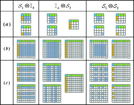
Figure 2: (Color online) Correlation matrices related to the families of $\rho$ for which the evolution equation of $D_{p}[\mathcal{S}(\rho)]$ is given by Eq. (8), with the Kraus operators of the channels being given respectively by (a) Eq. (30) with $i=1$, $j=2$, and $k=3$, (b) Eq. (39) with $k_{1}=1$, and (c) Eq. (40) with $k_{1}=1$, $k_{2}=4$, and $k_{3}=6$. Here, the correlation matrix elements denoted by the hollow squares should be zero, while those denoted by the color shaded squares can take arbitrary physically allowed values.

For clearness, we summarized in Fig. 2(a) the above results, where the correlation matrix is defined as

$$R=\left(\begin{array}[]{cc}\frac{1}{\sqrt{d_{A}d_{B}}}&y^{t}\\ x&T\\ \end{array}\right),$$ (33)

and the square lies in the $i$th row and $j$th column represents the corresponding correlation matrix elements.

Eq. (30) covers the depolarizing channel ($q_{0}=q$), and the bit flip ($i=1$), bit-phase flip ($i=2$), and phase flip ($i=3$) channels when $q_{0}=1$. It also enables one to identify those $\rho$ for which the correlations are immune of decay. For example, we have $\mathcal{S}_{1}^{\dagger}(\sigma_{1,2})=q\sigma_{1,2}$ and $\mathcal{S}_{1}^{\dagger}(\sigma_{3})=\sigma_{3}$ for the phase flip channel $\mathcal{S}_{1}\otimes\mathbb{I}_{2}$. Thus, if $x_{1,2}$ and the first two rows of $T$ in Eq. (2) equal zero, then $D_{p}[\mathcal{S}(\rho)]$, $\mathcal{N}_{\rm qt}[\mathcal{S}(\rho)]$, $\mathcal{F}_{\rm rsp}[\mathcal{S}(\rho)]$, and $\mathcal{B}_{\rm max}[\mathcal{S}(\rho)]$ will do not decay with time. Similar results can be obtained for the bit flip and bit-phase flip channels.

The channels of Eq. (30) are unital, i.e., $\mathcal{S}_{1}(\mathbb{I}_{2}/2)=\mathbb{I}_{2}/2$. We now further consider an nonunital channel, i.e., the generalized amplitude damping channel with

$$\begin{split}&E_{0}=\frac{1}{2}\sqrt{\eta_{\bar{n}}}[(1+q)\mathbb{I}_{2}-(1-q)\sigma_{3}],\\ &E_{1}=\frac{1}{2}\sqrt{\eta_{\bar{n}^{\prime}}}[(1+q)\mathbb{I}_{2}+(1-q)\sigma_{3}],\\ &E_{2}=\sqrt{\eta_{\bar{n}}}\sqrt{1-q^{2}}\sigma_{-},\\ &E_{3}=\sqrt{\eta_{\bar{n}^{\prime}}}\sqrt{1-q^{2}}\sigma_{+},\end{split}$$ (34)

where $\sigma_{\pm}=(\sigma_{1}\pm i\sigma_{2})/2$, $\eta_{\bar{n}^{\prime}}=1-\eta_{\bar{n}}$, and $\eta_{\bar{n}}$ is a parameter determined by the average thermal photons $\bar{n}$ in the reservoir thermal . When $\eta_{\bar{n}}=1$, one recovers the zero temperature reservoir, which has been discussed extensively with the Lorentzian, or the sub-Ohmic, Ohmic, and super-Ohmic type spectral densities dyn4 .

This generalized amplitude damping channel gives the map $\mathcal{S}_{1}^{\dagger}(\sigma_{1,2})=q\sigma_{1,2}$, and $\mathcal{S}_{1}^{\dagger}(\sigma_{3})=[1+2\eta_{\bar{n}}(q^{2}-1)]\mathbb{I}_{2}-2q^{2}|1\rangle\langle 1|$, with $|1\rangle$ being the lower energy state of $\sigma_{3}$. As a result, it also satisfies the conditions listed in Theorems 2 and 4, and thus the families of $\rho$ for which the evolution equations of $D_{p}[\mathcal{S}(\rho)]$ and $\tilde{D}_{p}[\mathcal{S}(\rho)]$ obey a factorization decay behavior can be obtained directly by using Eqs. (13) and (19).

IV.3 Gell-Mann channels

The Gell-Mann matrices are of the following form

$$\begin{split}&\lambda_{1}=\left(\begin{array}[]{ccc}0&1&0\\ 1&0&0\\ 0&0&0\end{array}\right),~{}\lambda_{2}=\left(\begin{array}[]{ccc}0&-i&0\\ i&0&0\\ 0&0&0\end{array}\right),\\ &\lambda_{3}=\left(\begin{array}[]{ccc}1&0&0\\ 0&-1&0\\ 0&0&0\end{array}\right),~{}\lambda_{4}=\left(\begin{array}[]{ccc}0&0&1\\ 0&0&0\\ 1&0&0\end{array}\right),\\ &\lambda_{5}=\left(\begin{array}[]{ccc}0&0&-i\\ 0&0&0\\ i&0&0\end{array}\right),~{}\lambda_{6}=\left(\begin{array}[]{ccc}0&0&0\\ 0&0&1\\ 0&1&0\end{array}\right),\\ &\lambda_{7}=\left(\begin{array}[]{ccc}0&0&0\\ 0&0&-i\\ 0&i&0\end{array}\right),~{}\lambda_{8}=\frac{1}{\sqrt{3}}\left(\begin{array}[]{ccc}1&0&0\\ 0&1&0\\ 0&0&-2\end{array}\right).\end{split}$$ (35)

The possible actions of the channel on a qutrit can be described by the Kraus operators that are linear combinations of the identity and the Gell-Mann matrices, and for convenience of presentation, we call them Gell-Mann channels. Similar as the qubit system, we consider here the representative class of $\mathcal{S}_{1}$ (with $\mathcal{S}_{2}$ being the same as $\mathcal{S}_{1}$, except that it acts on subsystem $b$) with the Kraus operators being given by

$$E_{0}=\sqrt{\varepsilon_{0}}\mathbb{I}_{3},~{}E_{k}=\sqrt{\varepsilon_{k}}\lambda_{k}~{}(k=\{1,2,\ldots,8\}),$$ (36)

where $\sum_{\mu=0}^{8}E_{\mu}^{\dagger}E_{\mu}=\mathbb{I}_{3}$.

Then, we suppose $\mathcal{S}_{1}^{\dagger}(\lambda_{k})=q_{k}\lambda_{k}$ for the purpose of finding the channel under the action of which the evolution equations of the correlation measures obey a factorization decay behavior. After a straightforward calculation, we obtain that the parameters $q_{k}$ must satisfy the following relations

$$\begin{split}&q_{1}+q_{2}+q_{3}=q_{6}+q_{7}+q_{8},\\ &q_{4}+q_{5}=q_{6}+q_{7},\end{split}$$ (37)

under which we have

$$\begin{split}&\varepsilon_{0}=\frac{1}{9}(1+3q_{6}+3q_{7}+2q_{8}),\\ &\varepsilon_{1}=\frac{1}{12}(2+6q_{1}-3q_{6}-3q_{7}-2q_{8}),\\ &\varepsilon_{2}=\frac{1}{12}(2+6q_{2}-3q_{6}-3q_{7}-2q_{8}),\\ &\varepsilon_{3}=\frac{1}{12}(2+6q_{3}-3q_{6}-3q_{7}-2q_{8}),\\ &\varepsilon_{4}=\frac{1}{12}(2+3q_{4}-3q_{5}-2q_{8}),\\ &\varepsilon_{5}=\frac{1}{12}(2-3q_{4}+3q_{5}-2q_{8}),\\ &\varepsilon_{6}=\frac{1}{12}(2+3q_{6}-3q_{7}-2q_{8}),\\ &\varepsilon_{7}=\frac{1}{12}(2-3q_{6}+3q_{7}-2q_{8}),\\ &\varepsilon_{8}=\frac{1}{12}(2-3q_{6}-3q_{7}+4q_{8}).\end{split}$$ (38)

The depolarizing channel for a qutrit can be considered as a special case of Eq. (36), which corresponds to $q_{k}=q$ for all $k=\{1,2,\ldots,8\}$. Moreover, by choosing $q_{k_{1},8}=1$ ($k_{1}=1$, $2$, or $3$), and $q_{k}=q$ for all $k\notin\{k_{1},8\}$, we present the class of the Gell-Mann channels with

$$\begin{split}&E_{0}=\sqrt{\frac{1+2q}{3}}\mathbb{I}_{3},~{}E_{1}=\sqrt{\frac{1-q}{2}}\lambda_{k_{1}},\\ &E_{2}=\sqrt{\frac{1-q}{2}}\lambda_{8},\end{split}$$ (39)

which gives $\mathcal{S}_{1}^{\dagger}(\lambda_{k})=\lambda_{k}$ for $k\in\{k_{1},8\}$, and $\mathcal{S}_{1}^{\dagger}(\lambda_{k})=q\lambda_{k}$ otherwise. Clearly, it satisfies the conditions listed in Theorems 2 and 4, and thus the families of $\rho$ for which the evolution equations of the considered correlations are governed by Eq. (8) can be found in Eqs. (13) and (19). See Fig. 2(b) for the related correlation matrices.

By choosing $q_{k_{1},k_{2},k_{3}}=q$ (here $k_{1}=1$, $2$, or $3$, $k_{2}=4$ or $5$, and $k_{3}=6$ or $7$), and $q_{k}=3q-2$ for all $k\notin\{k_{1},k_{2},k_{3}\}$, we present here another class of the Gell-Mann channels described by the Kraus operators

$$\begin{split}&E_{0}=(2q-1)\mathbb{I}_{3},~{}E_{1}=(1-q)\lambda_{k_{1}},\\ &E_{3}=(1-q)\lambda_{k_{2}},~{}E_{3}=(1-q)\lambda_{k_{3}},\end{split}$$ (40)

which gives the map $\mathcal{S}_{1}^{\dagger}(\lambda_{k})=q\lambda_{k}$ for $k\in\{k_{1},k_{2},k_{3}\}$, and $\mathcal{S}_{1}^{\dagger}(\lambda_{k})=(3q-2)\lambda_{k}$ otherwise. Thus, the families of $\rho$ for which $D_{p}[\mathcal{S}(\rho)]$ and $\tilde{D}_{p}[\mathcal{S}(\rho)]$ obey the factorization decay behavior can be obtained from Eqs. (13) and (19), respectively. See Fig. 2(c) for the related correlation matrices.

V Summary and discussion

In summary, we have investigated the evolution equations for a series of geometric correlation measures. These measures are all related with certain forms of the Schatten $p$-norm. We have established a simple relation that determines the evolution of these correlation measures. This relation is of central relevance for assessing the robustness of the related correlations which might be the resource of QIP tasks such as the input-output gate operation in sequential quantum computing and the experimental generation of quantum correlated resources in noisy environments. Moreover, as $\mathcal{S}(\rho)$ may represents the action of environment, of measurements, or of both on $\rho$, and the factorization decay behavior applies to various systems, various discord-like correlation measures, and even further various figures of merit associated with quantum teleportation, remote state preparation, and Bell-inequality violation, the criteria provided in this work are also useful for easing the evaluation of correlations in these tasks. A deep exploration of these relations might also be related with the structure of entanglement spectrum in describing topology of band structures of many-body systems haldane ; fan1 ; fan2 . We hope these results may shed some lights on understanding the essence of quantum correlations and their applications in QIP and condensed matter physics.

References

- (1) R. Horodecki, P. Horodecki, M. Horodecki, and K. Horodecki, Rev. Mod. Phys. 81, 865 (2009).
- (2) W. H. Zurek, Rev. Mod. Phys. 75, 715 (2003); M. Schlosshauer, ibid. 76, 1267 (2005); M. P. Almeida et al., Science 316, 579 (2007).
- (3) D. F. V. James, P. G. Kwiat, W. J. Munro, and A. G. White, Phys. Rev. A 64, 052312 (2001).
- (4) W. K. Wootters, Phys. Rev. Lett. 80, 2245 (1998).
- (5) T. Konrad, F. de Melo, M. Tiersch, C. Kasztelan, A. Aragão, and A. Buchleitner, Nat. Phys. 4, 99 (2008).
- (6) O. J. Farías, C. L. Latune, S. P. Walborn, L. Davidovich, and P. H. S. Ribeiro, Science 324, 1414 (2009).
- (7) M. Tiersch, F. de Melo, and A. Buchleitner, Phys. Rev. Lett. 101, 170502 (2008); G. Gour, ibid. 105, 190504 (2010).
- (8) Z. G. Li, S. M. Fei, Z. D. Wang, and W. M. Liu, Phys. Rev. A 79, 024303 (2009); Z. G. Li, M. J. Zhao, S. M. Fei, and W. M. Liu, ibid. 81, 042312 (2010).
- (9) J. G. Li, J. Zou, and B. Shao, Phys. Rev. A 82, 042318 (2010).
- (10) C. S. Yu, X. X. Yi, and H. S. Song, Phys. Rev. A 78, 062330 (2008).
- (11) Z. Liu and H. Fan, Phys. Rev. A 79, 032306 (2009).
- (12) S. Y. Mirafzali, I. Sargolzahi, A. Ahanj, K. Javidan, and M. Sarbishaei, Phys. Rev. A 82, 032321 (2010).
- (13) H. Ollivier and W. H. Zurek, Phys. Rev. Lett. 88, 017901 (2001); L. Henderson and V. Vedral, J. Phys. A 34, 6899 (2001).
- (14) B. Dakić, V. Vedral, and Č. Brukner, Phys. Rev. Lett. 105, 190502 (2010).
- (15) S. Luo and S. Fu, Phys. Rev. A 82, 034302 (2010).
- (16) F. M. Paula, T. R. de Oliveira, and M. S. Sarandy, Phys. Rev. A 87, 064101 (2013).
- (17) F. Ciccarello, T. Tufarelli, and V. Giovannetti, New J. Phys. 16, 013038 (2014).
- (18) D. Girolami, T. Tufarelli, and G. Adesso, Phys. Rev. Lett. 110, 240402 (2013).
- (19) L. Chang and S. Luo, Phys. Rev. A 87, 062303 (2013).
- (20) S. Luo and S. Fu, Phys. Rev. Lett. 106, 120401 (2011).
- (21) M. L. Hu and H. Fan, New J. Phys. 17, 033004 (2015).
- (22) A. Datta, A. Shaji, and C. M. Caves, Phys. Rev. Lett. 100, 050502 (2008).
- (23) B. Dakić et al., Nat. Phys. 8, 666 (2012).
- (24) M. Gu et al., Nat. Phys. 8, 671 (2012).
- (25) K. Modi, A. Brodutch, H. Cable, T. Paterek, and V. Vedral, Rev. Mod. Phys. 84, 1655 (2012).
- (26) A. Shabani and D. A. Lidar, Phys. Rev. Lett. 102, 100402 (2009); C. A. Rodríguez-Rosario, G. Kimura, H. Imai, and A. Aspuru-Guzik, ibid. 106, 050403 (2011); M. Gessner and H.-P. Breuer, ibid. 107, 180402 (2011).
- (27) L. Mazzola, J. Piilo, and S. Maniscalco, Phys. Rev. Lett. 104, 200401 (2010); L. S. Madsen, A. Berni, M. Lassen, and U. L. Andersen, ibid. 109, 030402 (2012).
- (28) J. S. Xu, X. Y. Xu, C. F. Li, C. J. Zhang, X. B. Zou, G. C. Guo, Nat. Commun. 1, 7 (2010).
- (29) T. Werlang, S. Souza, F. F. Fanchini, and C. J. Villas Boas, Phys. Rev. A 80, 024103 (2009); J. Maziero, L. C. Céleri, R. M. Serra, and V. Vedral, ibid. 80, 044102 (2009); J. Maziero, T. Werlang, F. F. Fanchini, L. C. Céleri, and R. M. Serra, ibid. 81, 022116 (2010); K. Berrada, F. F. Fanchini, and S. Abdel-Khalek, ibid. 85, 052315 (2012); B. Bellomo, R. L. Franco, and G. Compagno, ibid. 86, 012312 (2012).
- (30) B. Wang, Z. Y. Xu, Z. Q. Chen, and M. Feng, Phys. Rev. A 81, 014101 (2010); F. F. Fanchini, T. Werlang, C. A. Brasil, L. G. E. Arruda, and A. O. Caldeira, ibid. 81, 052107 (2010); M. L. Hu and H. Fan, Ann. Phys. (NY) 327, 2343 (2012).
- (31) B. Aaronson, R. L. Franco, G. Compagno, and G. Adesso, New J. Phys. 15, 093022 (2013); J. D. Montealegre, F. M. Paula, A. Saguia, and M. S. Sarandy, Phys. Rev. A 87, 042115 (2013); B. Aaronson, R. L. Franco, and G. Adesso, ibid. 88, 012120 (2013).
- (32) R. Horodecki, M. Horodecki, and P. Horodecki, Phys. Lett. A 222, 21 (1996).
- (33) R. Horodecki, P. Horodecki, and M. Horodecki, Phys. Lett. A 200, 340 (1995).
- (34) G. F. Zhang, A. L. Ji, H. Fan, and W. M. Liu, Ann. Phys. (NY) 327, 2074 (2012); H. Hao and L. F. Wei, Int. J. Theor. Phys. 52, 987 (2013); W. Song, L. B. Yu, P. Dong, D. C. Li, M. Yang, and Z. L. Cao, Sci. China Phys. Mech. 56, 737 (2013).
- (35) A. Bendersky, F. Pastawski, and J. P. Paz, Phys. Rev. Lett. 100, 190403 (2008); A. Chiuri, et al., ibid 107, 253602 (2011).
- (36) M. L. Hu, Ann. Phys. (NY) 327, 2332 (2012).
- (37) H. Li and F. D. M. Haldane, Phys. Rev. Lett. 101, 010504 (2008).
- (38) Z. Liu, E. J. Bergholtz, H. Fan, and A. M. Lauchli, Phys. Rev. Lett. 109, 186805 (2012).
- (39) D. Wang, Z. Liu, J. P. Cao, and H. Fan, Phys. Rev. Lett. 111, 186804 (2013).