Computing derivative-based global sensitivity measures using polynomial chaos expansions

Abstract

In the field of computer experiments sensitivity analysis aims at quantifying the relative importance of each input parameter (or combinations thereof) of a computational model with respect to the model output uncertainty. Variance decomposition methods leading to the well-known Sobol’ indices are recognized as accurate techniques, at a rather high computational cost though. The use of polynomial chaos expansions (PCE) to compute Sobol’ indices has allowed to alleviate the computational burden though. However, when dealing with large dimensional input vectors, it is good practice to first use screening methods in order to discard unimportant variables. The derivative-based global sensitivity measures (DGSM) have been developed recently in this respect. In this paper we show how polynomial chaos expansions may be used to compute analytically DGSMs as a mere post-processing. This requires the analytical derivation of derivatives of the orthonormal polynomials which enter PC expansions. The efficiency of the approach is illustrated on two well-known benchmark problems in sensitivity analysis.

url]http://www.ibk.ethz.ch/su/people/sudretb

1 Introduction

Nowadays, the increasing computing power allows one to use numerical models to simulate or predict the behavior of physical systems in various fields, e.g. mechanical engineering [1], civil engineering [2], chemistry [3], etc. The considered systems usually lead to highly complex models with numerous input factors (possibly tens to hundreds [4, 5]) that are required to represent all the parameters driving the system’s behaviour, e.g. boundary and initial conditions, material properties, external excitations, etc. On the one hand, this increases dramatically the computational cost. On the other hand, the input factors that are not perfectly known may introduce uncertainties into the predictions of the system response. In order to take into account the uncertainty, probabilistic approaches have been developed in the last two decades, in which the model input parameters are represented by random variables. Then the input uncertainties are propagated through the computational model and the distribution, moments or probability of exceeding prescribed thresholds may be computed [6, 7].

In this context, sensitivity analysis (SA) examines the sensitivity of the model output with respect to the input parameters, i.e. how the output variability is affected by the uncertain input factors [8, 9, 10]. The use of SA is common in various fields: engineering [2, 11, 1, 12], chemistry [3], nuclear safety [13], economy [14], biology [15], and medicine [16], among others. One can traditionally classify SA into local and global sensitivity analyses. The former aims at assessing the output sensitivity to small input perturbations around the nominal values of input parameters. The latter aims at assessing the overall or average influence of input parameters onto the output. Local SA has the disadvantages of being related to a fixed nominal point in the input space, and the interaction between the inputs is not accounted for [17]. On the other hand, global SA techniques take into account the input interaction and are not based on the choice of a nominal point but account for the whole input space.

The most common sensitivity analysis methods found in the literature are the method of [18], FAST [19, 20, 21] and variance decomposition methods originally investigated in [22, 23, 24, 25, 26, 27]. Usually standard Monte Carlo simulation (MCS) is employed for estimating the sensitivity indices in all these techniques. This approach requires a large number of model evaluations though and therefore is usually computationally expensive. When complex systems are of interest, the standard MCS becomes unaffordable. To overcome this problem, metamodels (also called surrogate models or emulators) are usually used in order to carry out the Monte Carlo simulation [28, 29]. In particular, polynomial chaos expansions (PCE) have been recognized as a versatile tool for building surrogate models and for conducting reliability and sensitivity analyses, as originally shown in [30, 31, 32]. Using PCE, variance-based sensitivity analysis becomes a mere post-processing of the polynomial coefficients once they have been computed.

More recently, a new gradient-based technique has been proposed for screening unimportant factors. The so-called derivative-based global sensitivity measures (DGSM) are shown to be upper bounds of the total Sobol’ indices while being less computationally demanding [33, 34, 17, 35]. Although the computational cost of this technique is reduced compared to the variance-based technique [17], its practical computation still relies on the Monte Carlo simulation approach.

In this paper we investigate the potential of polynomial chaos expansions for computing derivative-based sensitivity indices and allow for an efficient screening procedure. The paper is organized as follows: the classical derivation of Sobol’ indices and their link to derivative-based sensitivity indices is summarized in Section 2. The machinery of polynomial chaos expansions and the link with sensitivity analysis is developed in Section 3. The computation of the DGSM based on PC expansions is then presented in Section 4, in which an original method for computing the derivatives of orthogonal polynomials is presented. Finally two numerical tests are carried out in Section 5.

2 Derivative-based global sensitivity measures

2.1 Variance-based sensitivity measures

Global sensitivity analysis (SA) aims at quantifying the impact of input parameters onto the output quantities of interest. One input factor is considered insignificant (unessential) when it has little or no effect on the output variability. In practice, screening out the insignificant factors allows one to reduce the dimension of the problem, e.g. by fixing the unessential parameters.

Variance-based SA relies upon the decomposition of the output variance into contributions of different components, i.e. marginal effects and interactions of input factors. Consider a numerical model $Y={\mathcal{M}}(\boldsymbol{X})$ where the input vector $\boldsymbol{X}$ contains $M$ independent input variables $\boldsymbol{X}=\left\{X_{1},\,\dots\,,X_{M}\right\}$ with uniform distribution over the unit-hypercube ${\mathcal{H}}^{M}$ and $Y$ is the scalar output. The Sobol’ decomposition reads [22]:

$$\begin{split}Y={\mathcal{M}}(\boldsymbol{X})=&{\mathcal{M}}_{0}+\sum\limits_{i=1}^{M}{\mathcal{M}}_{i}(X_{i})+\sum\limits_{1\leq i<j\leq M}{\mathcal{M}}_{i,j}(X_{i},X_{j})+\dots\\ &+{\mathcal{M}}_{1,\,\dots\,,M}(X_{1},\,\dots\,,X_{M})\end{split}$$ (1)

in which ${\mathcal{M}}_{0}={\mathbb{E}}\left[{\mathcal{M}}(\boldsymbol{X})\right]$ is a constant term and each summand ${\mathcal{M}}_{i_{1},\,\dots\,,i_{s}}(X_{i_{1}}\allowbreak,\,\dots\,,X_{i_{s}})$ is a function of the variables $\left\{X_{i_{1}},\,\dots\,,X_{i_{s}}\right\},s\leq M$. For the sake of conciseness we introduce the following notation for the subset of indices:

$${\boldsymbol{\mathsf{u}}}\stackrel{{\scriptstyle\text{\tiny def}}}{{=}}\left\{i_{1},\,\dots\,,i_{s}\right\}$$ (2)

and denote by $\boldsymbol{X}_{{\boldsymbol{\mathsf{u}}}}$ the subvector of $\boldsymbol{X}$ that consists of the variables indexed by ${\boldsymbol{\mathsf{u}}}$. Using this set notation, Eq. (1) rewrites:

$$Y\stackrel{{\scriptstyle\text{\tiny def}}}{{=}}{\mathcal{M}}_{0}+\sum_{\begin{subarray}{c}{\boldsymbol{\mathsf{u}}}\subset\left\{1,\,\dots\,,M\right\}\\ {\boldsymbol{\mathsf{u}}}\neq\boldsymbol{0}\end{subarray}}{\mathcal{M}}_{{\boldsymbol{\mathsf{u}}}}(\boldsymbol{X}_{{\boldsymbol{\mathsf{u}}}}),$$ (3)

in which ${\mathcal{M}}_{{\boldsymbol{\mathsf{u}}}}(\boldsymbol{X}_{{\boldsymbol{\mathsf{u}}}})$ is the summand including the subset of parameters $\boldsymbol{X}_{{\boldsymbol{\mathsf{u}}}}$. According to [22], a unique decomposition requires the orthogonality of the summands, i.e.:

$${\mathbb{E}}\left[{\mathcal{M}}_{{\boldsymbol{\mathsf{u}}}}(\boldsymbol{X}_{{\boldsymbol{\mathsf{u}}}})\,{\mathcal{M}}_{{\boldsymbol{\mathsf{v}}}}(\boldsymbol{X}_{{\boldsymbol{\mathsf{v}}}})\right]=\int_{{\mathcal{H}}^{M}}{\mathcal{M}}_{{\boldsymbol{\mathsf{u}}}}(\boldsymbol{x}_{{\boldsymbol{\mathsf{u}}}})\,{\mathcal{M}}_{{\boldsymbol{\mathsf{v}}}}(\boldsymbol{x}_{{\boldsymbol{\mathsf{v}}}})\,{\rm d}\boldsymbol{x}=0\quad,\quad{\boldsymbol{\mathsf{u}}}\neq{\boldsymbol{\mathsf{v}}}$$ (4)

In particular each summand shall be of zero mean value. Accordingly the variance of the response $Y={\mathcal{M}}(\boldsymbol{X})$ reads:

$$D\stackrel{{\scriptstyle\text{\tiny def}}}{{=}}{\rm Var}\left[Y\right]=\sum\limits_{\begin{subarray}{c}{\boldsymbol{\mathsf{u}}}\subset\left\{1,\,\dots\,,M\right\}\\ {\boldsymbol{\mathsf{u}}}\neq\boldsymbol{0}\end{subarray}}{\rm Var}\left[{\mathcal{M}}_{{\boldsymbol{\mathsf{u}}}}(\boldsymbol{X}_{{\boldsymbol{\mathsf{u}}}})\right].$$ (5)

In this expansion ${\rm Var}\left[{\mathcal{M}}_{{\boldsymbol{\mathsf{u}}}}(\boldsymbol{X}_{{\boldsymbol{\mathsf{u}}}})\right]$ is the contribution of summand ${\mathcal{M}}(\boldsymbol{X}_{{\boldsymbol{\mathsf{u}}}})$ to the output variance.

The Sobol’ sensitivity index $S_{{\boldsymbol{\mathsf{u}}}}$ for the subset of variables $\boldsymbol{X}_{{\boldsymbol{\mathsf{u}}}}$ is defined as follows [23]:

$$S_{{\boldsymbol{\mathsf{u}}}}\stackrel{{\scriptstyle\text{\tiny def}}}{{=}}\dfrac{D_{{\boldsymbol{\mathsf{u}}}}}{D}=\dfrac{{\rm Var}\left[{\mathcal{M}}_{{\boldsymbol{\mathsf{u}}}}(\boldsymbol{X}_{{\boldsymbol{\mathsf{u}}}})\right]}{D}$$ (6)

The total sensitivity index for subset $\boldsymbol{X}_{{\boldsymbol{\mathsf{u}}}}$ is given by [23]:

$$S_{{\boldsymbol{\mathsf{u}}}}^{T}\stackrel{{\scriptstyle\text{\tiny def}}}{{=}}\dfrac{D_{{\boldsymbol{\mathsf{u}}}}^{T}}{D}=\sum\limits_{{\boldsymbol{\mathsf{v}}}\supset{\boldsymbol{\mathsf{u}}}}\dfrac{{\rm Var}\left[{\mathcal{M}}_{{\boldsymbol{\mathsf{v}}}}(\boldsymbol{X}_{{\boldsymbol{\mathsf{v}}}})\right]}{D}$$ (7)

where the sum is extended over all sets ${\boldsymbol{\mathsf{v}}}=\left\{j_{1},\,\dots\,,j_{t}\right\}$ which contains ${\boldsymbol{\mathsf{u}}}$. It represents the total amount of uncertainty apportioned to the subset of variables $\boldsymbol{X}_{{\boldsymbol{\mathsf{u}}}}$. For instance, for a single variable $X_{i},\,i=1,\,\dots\,,M$ the Sobol’ sensitivity index reads:

$$S_{i}=\dfrac{{\rm Var}\left[{\mathcal{M}}_{i}(X_{i})\right]}{D},$$ (8)

and the total Sobol’ sensitivity index reads:

$$S_{i}^{T}=\sum\limits_{{\boldsymbol{\mathsf{v}}}\ni i}\dfrac{{\rm Var}\left[{\mathcal{M}}_{{\boldsymbol{\mathsf{v}}}}(\boldsymbol{X}_{{\boldsymbol{\mathsf{v}}}})\right]}{D}.$$ (9)

$S_{i}$ and $S_{i}^{T}$ respectively represent the sole and total effect of the factor $X_{i}$ on the system’s output variability. The smaller $S_{i}^{T}$ is, the less important the factor $X_{i}$ is. In the case when $S_{i}^{T}\ll 1$, $X_{i}$ is considered as unimportant (unessential or insignificant) and may be replaced in the analysis by a deterministic value.

In the literature one can find different approaches for computing the total Sobol’ indices, such as the Monte Carlo simulation (MCS) and the spectral approach. [22, 23] proposed direct estimation of the sensitivity indices for subsets of variables using only the model evaluations at specially selected points. The approach relies on computing analytically the integral representations of $D_{{\boldsymbol{\mathsf{u}}}}$ and $D_{{\boldsymbol{\mathsf{u}}}}^{T}$ respectively defined in Eq. (6) and Eq. (7).

Let us denote by $\overline{{\boldsymbol{\mathsf{u}}}}$ the set that is complementary to ${\boldsymbol{\mathsf{u}}}$, i.e. $\boldsymbol{X}=(\boldsymbol{X}_{{\boldsymbol{\mathsf{u}}}},\boldsymbol{X}_{\overline{{\boldsymbol{\mathsf{u}}}}})$. Let $\boldsymbol{X}$ and $\boldsymbol{X}^{\prime}$ be vectors of independent uniform variables defined on the unit hypercube ${\mathcal{H}}^{M}$ and define $\boldsymbol{X}^{\prime}=(\boldsymbol{X}_{{\boldsymbol{\mathsf{u}}}}^{{}^{\prime}},\boldsymbol{X}_{\overline{{\boldsymbol{\mathsf{u}}}}}^{{}^{\prime}})$. The partial variance $D_{{\boldsymbol{\mathsf{u}}}}$ is represented as follows [24]:

$$D_{{\boldsymbol{\mathsf{u}}}}=\iint{\mathcal{M}}(\boldsymbol{x}){\mathcal{M}}(\boldsymbol{x}_{{\boldsymbol{\mathsf{u}}}},\boldsymbol{x}_{\overline{{\boldsymbol{\mathsf{u}}}}}^{{}^{\prime}})\,{\rm d}\boldsymbol{x}\;{\rm d}\boldsymbol{x}_{\overline{{\boldsymbol{\mathsf{u}}}}}^{{}^{\prime}}-{{\mathcal{M}}_{0}}^{2}$$ (10)

The total variance $D_{{\boldsymbol{\mathsf{u}}}}^{T}$ is given by [24]:

$$D_{{\boldsymbol{\mathsf{u}}}}^{T}=\dfrac{1}{2}\iint\left[{\mathcal{M}}(\boldsymbol{x})-{\mathcal{M}}(\boldsymbol{x}_{{\boldsymbol{\mathsf{u}}}}^{{}^{\prime}},\boldsymbol{x}_{\overline{{\boldsymbol{\mathsf{u}}}}})\right]^{2}\,{\rm d}\boldsymbol{x}\;{\rm d}\boldsymbol{x}_{\overline{{\boldsymbol{\mathsf{u}}}}}$$ (11)

A Monte Carlo algorithm is used to estimate the above integrals. For each sample point, one generates two $M$-dimensional samples $\boldsymbol{x}=({\boldsymbol{x}_{{\boldsymbol{\mathsf{u}}}}},{\boldsymbol{x}_{\overline{{\boldsymbol{\mathsf{u}}}}}})$ and $\boldsymbol{x}^{{}^{\prime}}=({\boldsymbol{x}_{{\boldsymbol{\mathsf{u}}}}}^{{}^{\prime}},{\boldsymbol{x}_{\overline{{\boldsymbol{\mathsf{u}}}}}}^{{}^{\prime}})$. The function is evaluated at three points $({\boldsymbol{x}_{{\boldsymbol{\mathsf{u}}}}},{\boldsymbol{x}_{\overline{{\boldsymbol{\mathsf{u}}}}}})$, $(\boldsymbol{x}_{{\boldsymbol{\mathsf{u}}}}^{{}^{\prime}},{\boldsymbol{x}_{\overline{{\boldsymbol{\mathsf{u}}}}}})$ and $({\boldsymbol{x}_{{\boldsymbol{\mathsf{u}}}}},\boldsymbol{x}_{\overline{{\boldsymbol{\mathsf{u}}}}}^{{}^{\prime}})$. Using $N$ independent sample points, one computes the quantities of interest $D$, $D_{{\boldsymbol{\mathsf{u}}}}$ and $D_{{\boldsymbol{\mathsf{u}}}}^{T}$ by means of the following crude Monte Carlo estimators:

$${\mathcal{M}}_{0}=\dfrac{1}{N}\sum\limits_{i=1}^{N}{\mathcal{M}}\left(\boldsymbol{x}^{(i)}\right)$$ (12)

$$D+{{\mathcal{M}}_{0}}^{2}=\dfrac{1}{N}\sum\limits_{i=1}^{N}\left[{\mathcal{M}}\left(\boldsymbol{x}^{(i)}\right)\right]^{2}$$ (13)

$$D_{{\boldsymbol{\mathsf{u}}}}+{{\mathcal{M}}_{0}}^{2}=\dfrac{1}{N}\sum\limits_{i=1}^{N}{\mathcal{M}}\left(\boldsymbol{x}^{(i)}\right){\mathcal{M}}\left({\boldsymbol{x}_{{\boldsymbol{\mathsf{u}}}}^{(i)}},{\boldsymbol{x}_{\overline{{\boldsymbol{\mathsf{u}}}}}^{{(i)}^{\prime}}}\right)$$ (14)

$$D_{{\boldsymbol{\mathsf{u}}}}^{T}=\dfrac{1}{N}\sum\limits_{i=1}^{N}\dfrac{1}{2}\left[{\mathcal{M}}\left(\boldsymbol{x}^{(i)}\right)-{\mathcal{M}}\left({\boldsymbol{x}_{{\boldsymbol{\mathsf{u}}}}^{{(i)}^{\prime}}},{\boldsymbol{x}_{\overline{{\boldsymbol{\mathsf{u}}}}}^{(i)}}\right)\right]^{2}$$ (15)

The computation of the sensitivity indices by MCS may exhibit reduced accuracy when the mean value ${\mathcal{M}}_{0}$ is large. In addition, the computational cost is prohibitive: in order to compute the sensitivity indices for $M$ parameters, MCS requires $(M+2)\times N$ model runs, in which $N$ is the number of sample points typically chosen equal to $10^{3}-10^{4}$ to reach an acceptable accuracy. [26] suggested a procedure that is more efficient for computing the first and total sensitivity indices. [36] modified the MCS procedure in order to reduce the lack of accuracy. Some other estimators for the sensitivity indices by MCS may be found in [37, 38].

2.2 Derivative-based sensitivity indices

The total Sobol’ indices may be used for screening purposes. Indeeed a negligible total Sobol’ index $S_{i}^{T}$ means that variable $X_{i}$ does not contribute to the output variance, neither directly nor in interaction with orther variables. In order to avoid the computational burden associated with estimating all total Sobol’ indices, a new technique based on derivatives has been recently proposed by [17].

Derivative-based sensitivity analysis originates from the Morris method introduced in [18]. The idea is to measure the average of the elementary effects over the input space. Considering variable $X_{i}$ one first samples an experimental design (ED) in the input space ${\mathcal{X}}=\left\{\boldsymbol{x}^{(1)},\,\dots\,,\boldsymbol{x}^{(N)}\right\}$ and then varies this sample in the $i^{th}$ direction. The elementary effect ($EE$) is defined as:

$$EE_{i}^{(j)}=\dfrac{{\mathcal{M}}(\boldsymbol{x}_{r}^{(j)})-{\mathcal{M}}(\boldsymbol{x}^{(j)})}{\Delta}$$ (16)

in which $\boldsymbol{x}^{(j)}=\left\{x_{1}^{(j)},\,\dots\,,x_{i}^{(j)},\,\dots\,,x_{M}^{(j)}\right\}$ is the $j^{th}$ sample point and $\boldsymbol{x}_{r}^{(j)}=\left\{x_{1}^{(j)},\,\dots\,,x_{i}^{(j)}+\Delta,\,\dots\,,x_{M}^{(j)}\right\}$ is the perturbed sample point in the $i$-th direction. The Morris importance measure (Morris factor) is defined as the average of the $EE_{i}$’s:

$$\mu_{i}=\dfrac{1}{N}\sum\limits_{j=1}^{N}EE_{i}^{(j)}$$ (17)

By definition, the variance $\sigma_{i}^{2}$ of the $EE$s is calculated from:

$$\sigma_{i}^{2}=\dfrac{1}{N-1}\sum\limits_{j=1}^{N}(EE_{i}^{(j)}-\mu_{i})^{2}$$ (18)

Kucherenko et al. [17] generalized these quantities as follows:

$$\mu_{i}\stackrel{{\scriptstyle\text{\tiny def}}}{{=}}{\mathbb{E}}\left[\dfrac{\partial{\mathcal{M}}}{\partial x_{i}}(\boldsymbol{X})\right]=\int_{{\mathcal{H}}^{M}}\dfrac{\partial{\mathcal{M}}}{\partial x_{i}}(\boldsymbol{x}){\rm d}\boldsymbol{x}$$ (19)

$$\sigma_{i}^{2}=\int\limits_{{\mathcal{H}}^{M}}\left[\dfrac{\partial{\mathcal{M}}}{\partial x_{i}}(\boldsymbol{x})\right]^{2}\,{\rm d}\boldsymbol{x}-\mu_{i}^{2}$$ (20)

provided that $\dfrac{\partial{\mathcal{M}}}{\partial x_{i}}$ is square-integrable. Any input parameter $X_{i}$ with $\mu_{i}\ll 1$ and $\sigma_{i}\ll 1$ is considered as unimportant. It has been shown that the Morris factor has a higher convergence rate compared to variance-based methods, which makes it attractive from a computational viewpoint. Because the elementary effects may be positive or negative, they can cancel each other, which might lead to a misinterpretation of the importance of $X_{i}$. To avoid this, Campolongo et al. [3] modified the Morris factor as follows:

$$\mu_{i}^{\ast}={\mathbb{E}}\left[\left|\dfrac{\partial{\mathcal{M}}}{\partial x_{i}}(\boldsymbol{X})\right|\right]$$ (21)

Recently, Sobol’ and Kucherenko [33] introduced a new sensitivity measure (SM) which is the mean-squared derivative of the model with respect to $X_{i}$:

$$\nu_{i}={\mathbb{E}}\left[\left(\dfrac{\partial{\mathcal{M}}}{\partial x_{i}}(\boldsymbol{X})\right)^{2}\right]$$ (22)

Sobol’ and Kucherenko [33] and Lamboni et al. [35] could establish a link between the $\nu_{i}$ in Eq. (22) and the total Sobol’ indices in Eq. (9). In case $X_{i}$ is a uniform random variable over $[0,\,1]$, one gets:

$$S_{i}^{T}\leq S_{i}^{DGSM}\stackrel{{\scriptstyle\text{\tiny def}}}{{=}}\dfrac{\nu_{i}}{\pi^{2}D}$$ (23)

where $S_{i}^{DGSM}$ is the upper-bound to the total sensitivity index $S_{i}^{T}$ and $D$ is the model output variance. In case of a uniform variable $X_{i}\sim[a_{i},\,b_{i}]$ this upper bound scales to:

$$S_{i}^{T}\leq S_{i}^{DGSM}=\dfrac{(b_{i}-a_{i})^{2}}{\pi^{2}}\dfrac{\nu_{i}}{D}$$ (24)

Finally the above results can be extended to other types of distributions. If $X_{i}\sim{\mathcal{N}}\left(a_{i},b_{i}\right)$ is a Gaussian random variable with mean and variance $a_{i}$ and $b_{i}^{2}$ respectively, one gets:

$$S_{i}^{T}\leq S_{i}^{DGSM}={b_{i}}^{2}\dfrac{\nu_{i}}{D}$$ (25)

In the general case, Lamboni et al. [35] define the upper bound of the total Sobol’ index of $X_{i}$ as:

$$S_{i}^{DGSM}=4{C_{i}}^{2}\dfrac{\nu_{i}}{D}$$ (26)

in which $C_{i}=\sup\limits_{\begin{subarray}{c}x\in{\mathbb{R}}\end{subarray}}\dfrac{\min{\left[F_{X_{i}}(x),1-F_{X_{i}}(x)\right]}}{f_{X_{i}}(x)}$ is the Cheeger constant, $F_{X_{i}}$ is the cumulative distribution function of $X_{i}$ and $f_{X_{i}}$ is the probability density function of $X_{i}$.

3 Polynomial chaos expansions

Let us consider a numerical model $Y={\mathcal{M}}(\boldsymbol{X})$ where the input vector $\boldsymbol{X}$ is composed of $M$ independent random variables $\boldsymbol{X}=\left\{X_{i},\,i=1,\,\dots\,,M\right\}$ and $Y$ is the output quantity of interest. Assuming that $Y$ has a finite variance, it can be represented as follows [39, 40]:

$$Y={\mathcal{M}}(\boldsymbol{X})=\sum\limits_{j=0}^{\infty}y_{j}\phi_{j}(\boldsymbol{X})$$ (27)

in which $\left\{\phi_{j}(\boldsymbol{X}),j=0,\,\dots\,,\infty\right\}$ form a basis on the space of second order random variables and $y_{j}$’s are the coordinates of $Y$ onto this basis. In case the basis terms are multivariate orthonormal polynomials of the input variables $\boldsymbol{X}$, Eq. (27) is called polynomial chaos expansion.

Assuming that the input vector $\boldsymbol{X}$ has independent components $X_{i}$ with prescribed probability distribution functions $f_{X_{i}}$, one obtains the joint probability density function:

$$f_{\boldsymbol{X}}(\boldsymbol{x})=\prod\limits_{i=1}^{M}f_{X_{i}}(x_{i})$$ (28)

For each $X_{i}$, one can construct a family of orthogonal univariate polynomials $\left\{P_{k}^{(i)},k\in{\mathbb{N}}\right\}$ with respect to the probability measure ${\mathbb{P}}_{X_{i}}({\rm d}x_{i})=f_{X_{i}}(x_{i}){\rm d}x_{i}$ satifying:

$$\langle P_{j}^{(i)},P_{k}^{(i)}\rangle\stackrel{{\scriptstyle\text{\tiny def}}}{{=}}{\mathbb{E}}\left[P_{j}^{(i)}(X_{i})P_{k}^{(i)}(X_{i})\right]=\int P_{j}^{(i)}(x_{i})P_{k}^{(i)}(x_{i})f_{X_{i}}(x_{i}){\rm d}x_{i}=c_{j}^{(i)}\delta_{jk}$$ (29)

where $\langle\cdot,\cdot\rangle$ is the inner product defined on the space associated with the probability measure ${\mathbb{P}}_{X_{i}}({\rm d}x_{i})$, $\delta_{jk}$ is the Kronecker symbol with $\delta_{jk}=1$ if $j=k$, otherwise $\delta_{jk}=0$ and $c_{j}^{(i)}$ is a constant. The univariate polynomial $P_{j}^{(i)}$ belongs to a specific class according to the distribution of $X_{i}$. For instance, if $X_{i}$ is standard uniform (resp. Gaussian) random variable, $\left\{P_{j}^{(i)}\right\}_{j\geq 0}$ are orthogonal Legendre (resp. Hermite) polynomials. Then the orthonormal univariate polynomials are obtained by normalization:

$$\Psi_{j}^{(i)}=P_{j}^{(i)}/\sqrt{c_{j}^{(i)}}$$ (30)

Introducing the multi-indices $\boldsymbol{\alpha}=(\alpha_{1},\,\dots\,,\alpha_{M})$, a multivariate polynomial can be defined by tensor product as:

$$\Psi_{\boldsymbol{\alpha}}(\boldsymbol{x})\stackrel{{\scriptstyle\text{\tiny def}}}{{=}}\prod\limits_{i=1}^{M}\Psi_{\alpha_{i}}^{(i)}(x_{i})$$ (31)

Soize and Ghanem [40] prove that the set of all multivariate polynomials $\Psi_{\boldsymbol{\alpha}}$ in the input random vector $\boldsymbol{X}$ forms a basis of the Hilbert space of second order random variables:

$$Y=\sum\limits_{\boldsymbol{\alpha}\in{{\mathbb{N}}}^{M}}a_{\boldsymbol{\alpha}}\Psi_{\boldsymbol{\alpha}}(\boldsymbol{X})$$ (32)

where $a_{\boldsymbol{\alpha}}$’s are the deterministic coefficients of the representation.

In practice, the input random variables are usually not standardized, therefore it is necessary to transform the input vector into a set of standard variables. We define the isoprobabilistic transform $\boldsymbol{Z}={\mathcal{T}}^{-1}(\boldsymbol{X})$ which is a unique mapping from the original random space of $X_{i}$’s onto a standard space of $M$ basic independent random variables $Z_{i}$’s. As an example $Z_{i}$ may be a standard normal random variable or a uniform variable over $[-1,1]$.

In engineering applications, only a finite number of terms can be computed in Eq.(32). Accordingly, the truncated polynomial chaos expansion of $Y$ can be represented as follows [6]:

$$Y={\mathcal{M}}(\boldsymbol{X})={\mathcal{M}}\left({\mathcal{T}}(\boldsymbol{Z})\right)=\sum\limits_{\boldsymbol{\alpha}\in{\mathcal{A}}}a_{\boldsymbol{\alpha}}\Psi_{\boldsymbol{\alpha}}(\boldsymbol{Z})$$ (33)

in which ${\mathcal{A}}$ is the set of multi-indices $\boldsymbol{\alpha}$’s retained by the truncation scheme.

The application of PCE consists in choosing a suitable polynomial basis and then computing the appropriate coefficients $a_{\boldsymbol{\alpha}}$’s. To this end, there exist several techniques including spectral projection [41, 42], stochastic collocation method [43] or least square analysis (also called regression, see [44, 45]). A review of these so-called non-intrusive techniques is given in [46]. Recently, the least-square approach has been extended to obtain sparse expansions [47, 48]. This technique has been applied to global sensitivity analysis in [32]. The main results are now summarized.

First note that the orthonormality of the polynomial basis leads to the following properties:

$${\mathbb{E}}\left[\Psi_{\boldsymbol{\alpha}}(\boldsymbol{Z})\right]=0\qquad\text{and}\qquad{\mathbb{E}}\left[\Psi_{\boldsymbol{\alpha}}(\boldsymbol{Z})\,\Psi_{\boldsymbol{\beta}}(\boldsymbol{Z})\right]=\delta_{\boldsymbol{\alpha}\boldsymbol{\beta}}$$ (34)

As a consequence the mean value of the model output $y$ is ${\mathbb{E}}\left[Y\right]=a_{0}$ whereas the variance is the sum of the square of the other coefficients:

$$D={\rm Var}\left[Y\right]={\rm Var}\left[\sum\limits_{\boldsymbol{\alpha}\in{\mathcal{A}}}a_{\boldsymbol{\alpha}}\Psi_{\boldsymbol{\alpha}}(\boldsymbol{Z})\right]=\sum\limits_{\begin{subarray}{c}\boldsymbol{\alpha}\in{\mathcal{A}}\\ \boldsymbol{\alpha}\neq\boldsymbol{0}\end{subarray}}{a_{\boldsymbol{\alpha}}}^{2}\,{\rm Var}\left[\Psi_{\boldsymbol{\alpha}}(\boldsymbol{Z})\right]=\sum\limits_{\begin{subarray}{c}\boldsymbol{\alpha}\in{\mathcal{A}}\\ \boldsymbol{\alpha}\neq\boldsymbol{0}\end{subarray}}{a_{\boldsymbol{\alpha}}}^{2}$$ (35)

Making use of the unique orthonormality properties of the basis, Sudret [30, 31] proposed an original post-processing of the PCE for performing global sensitivity analysis. For any subset variables ${\boldsymbol{\mathsf{u}}}=\left\{i_{1},\,\dots\,,i_{s}\right\}\subset\left\{1,\,\dots\,,M\right\}$, one defines the set of multivariate polynomials $\Psi_{\boldsymbol{\alpha}}$ which depends only on ${\boldsymbol{\mathsf{u}}}$:

$${\mathcal{A}}_{{\boldsymbol{\mathsf{u}}}}=\left\{\boldsymbol{\alpha}\in{\mathcal{A}}:\alpha_{k}\neq 0\,\text{if and only if}\,k\in{\boldsymbol{\mathsf{u}}}\right\}$$ (36)

The ${\mathcal{A}}_{{\boldsymbol{\mathsf{u}}}}$’s form a partition of ${\mathcal{A}}$, thus the Sobol’ decomposition of the truncated PCE in Eq. (33) may be written as follows:

$$Y=a_{0}+\sum\limits_{\begin{subarray}{c}{\boldsymbol{\mathsf{u}}}\subset\left\{1,\,\dots\,,M\right\}\\ {\boldsymbol{\mathsf{u}}}\neq\emptyset\end{subarray}}{\mathcal{M}}_{{\boldsymbol{\mathsf{u}}}}(\boldsymbol{Z}_{{\boldsymbol{\mathsf{u}}}})$$ (37)

where:

$${\mathcal{M}}_{{\boldsymbol{\mathsf{u}}}}(\boldsymbol{Z}_{{\boldsymbol{\mathsf{u}}}})\stackrel{{\scriptstyle\text{\tiny def}}}{{=}}\sum\limits_{\boldsymbol{\alpha}\in{\mathcal{A}}_{{\boldsymbol{\mathsf{u}}}}}a_{\boldsymbol{\alpha}}\Psi_{\boldsymbol{\alpha}}(\boldsymbol{Z})$$ (38)

In other words the Sobol’ decomposition is directly read from the PC expansion. Consequently, due to the orthonormality of PC basis, the partial variance $D_{{\boldsymbol{\mathsf{u}}}}$ reads:

$$D_{{\boldsymbol{\mathsf{u}}}}={\rm Var}\left[{\mathcal{M}}_{{\boldsymbol{\mathsf{u}}}}(\boldsymbol{Z}_{{\boldsymbol{\mathsf{u}}}})\right]=\sum\limits_{\boldsymbol{\alpha}\in{\mathcal{A}}_{{\boldsymbol{\mathsf{u}}}}}a_{\boldsymbol{\alpha}}^{2}$$ (39)

As a cosequence the Sobol’ indices at any order may be computed by a mere combination of the squares of the coefficients. As an illustration, the first order PC-based Sobol’ indices read:

$$S_{i}=\sum\limits_{\boldsymbol{\alpha}\in{\mathcal{A}}_{i}}a_{\boldsymbol{\alpha}}^{2}/D,\quad{\mathcal{A}}_{i}=\left\{\boldsymbol{\alpha}\in{\mathcal{A}}:\alpha_{i}>0,\,\alpha_{j\neq i}=0\right\}$$ (40)

whereas the total PC-based Sobol’ indices are:

$$S_{i}^{T}=\sum\limits_{\boldsymbol{\alpha}\in{\mathcal{A}}_{i}^{T}}a_{\boldsymbol{\alpha}}^{2}/D,\quad{\mathcal{A}}_{i}^{T}=\left\{\boldsymbol{\alpha}\in{\mathcal{A}}:\alpha_{i}>0\right\}$$ (41)

4 Derivative of polynomial chaos expansions

In this paper, we consider the combination of polynomial chaos expansions with derivative-based global sensitivity analysis. On the one hand, PCE are already known to provide accurate metamodels at reasonable cost. On the other hand, the derivative-based sensitivity measure (DGSM) is effective for screening unimportant input factors. The combination of PCE and DGSM appears as a promising approach for effective low-cost SA. In fact, once the PCE metamodel is built, the DGSM can be computed as a mere post-processing of the metamodel which simply consists of polynomial functions.

As seen in Section 2, a DGSM is related to the expectation of the square of the model derivative, which was denoted by $\nu_{i}$. We will express the model derivative in a way such that the expectation operator can be easily computed, more precisely by projecting the components of the gradient $\nabla{\mathcal{M}}$ onto a PC expansion.

4.1 Hermite polynomial chaos expansions

In this section we consider a numerical model $Y={\mathcal{M}}(\boldsymbol{X})$ where $Y$ is the scalar output and $\boldsymbol{X}=\left\{X_{i},\,\dots\,,X_{M}\right\}$ is the input vector composed of $M$ independent Gaussian variables $X_{i}\sim{\mathcal{N}}\left(\mu_{i},\sigma_{i}\right)$. The isoprobabilistic transform reads:

$$\boldsymbol{X}={\mathcal{T}}(\boldsymbol{Z}):\qquad X_{i}=\mu_{i}+\sigma_{i}Z_{i}$$ (42)

where $Z_{i}\sim{\mathcal{N}}(0,1)$ are standard normal random variables. The truncated PCE of $Y$ reads:

$$Y={\mathcal{M}}(\boldsymbol{X})={\mathcal{M}}\left({\mathcal{T}}(\boldsymbol{Z})\right)=\sum\limits_{\boldsymbol{\alpha}\in{\mathcal{A}}}a_{\boldsymbol{\alpha}}\Psi_{\boldsymbol{\alpha}}(\boldsymbol{Z})$$ (43)

in which $\boldsymbol{\alpha}=\left\{\alpha_{1},\,\dots\,,\alpha_{M}\right\}$ is a multi-index, ${\mathcal{A}}$ is the set of indices $\boldsymbol{\alpha}$ in the truncated expansion, $\Psi_{\boldsymbol{\alpha}}(\boldsymbol{z})=\prod\limits_{i=1}^{M}\tilde{He}_{\alpha_{i}}(z_{i})$ is the multivariate polynomial basis obtained as the tensor product of univariate orthonormal Hermite polynomials $\tilde{He}_{\alpha_{i}}(z_{i})$ (see A) and $a_{\boldsymbol{\alpha}}$ is the deterministic coefficient associated with $\Psi_{\boldsymbol{\alpha}}(\boldsymbol{z})$.

Since ${\mathcal{T}}$ is a one-to-one mapping with $\dfrac{\partial z_{i}}{\partial x_{i}}=\dfrac{1}{\sigma_{i}}$, the derivative-based sensitivity index reads:

$$\nu_{i}={\mathbb{E}}\left[\left(\dfrac{\partial{\mathcal{M}}}{\partial x_{i}}(\boldsymbol{X})\right)^{2}\right]={\mathbb{E}}\left[\left(\dfrac{\partial{\mathcal{M}}\circ{\mathcal{T}}}{\partial z_{i}}\dfrac{\partial z_{i}}{\partial x_{i}}\right)^{2}\right]=\dfrac{1}{{\sigma_{i}}^{2}}{\mathbb{E}}\left[\left(\dfrac{\partial{\mathcal{M}}\circ{\mathcal{T}}}{\partial z_{i}}(\boldsymbol{Z})\right)^{2}\right]$$ (44)

The DGSM of $X_{i}$, in other words the corresponding upper bound to the total Sobol’ index $S_{i}^{T}$, is computed according to Eq. (25):

$$S_{i}^{DGSM}=\sigma_{i}^{2}\dfrac{\nu_{i}}{D}=\dfrac{1}{D}{\mathbb{E}}\left[\left(\dfrac{\partial{\mathcal{M}}\circ{\mathcal{T}}}{\partial z_{i}}(\boldsymbol{Z})\right)^{2}\right]=\dfrac{1}{D}{\mathbb{E}}\left[\left(\dfrac{\partial}{\partial z_{i}}\sum\limits_{\boldsymbol{\alpha}\in{\mathcal{A}}}a_{\boldsymbol{\alpha}}\Psi_{\boldsymbol{\alpha}}(\boldsymbol{Z})\right)^{2}\right]$$ (45)

in which $D={\rm Var}\left[Y\right]=\sum\limits_{\boldsymbol{\alpha}\in{\mathcal{A}},\,\boldsymbol{\alpha}\neq\boldsymbol{0}}a_{\boldsymbol{\alpha}}^{2}$. This requires computing the partial derivatives of polynomial functions of the form ${\mathcal{M}}_{{\mathcal{A}}}(\boldsymbol{z})=\sum\limits_{\boldsymbol{\alpha}\in{\mathcal{A}}}a_{\boldsymbol{\alpha}}\Psi_{\boldsymbol{\alpha}}(\boldsymbol{z})$. One can prove that the derivatives $\tilde{He}_{n}^{{}^{\prime}}(z)=\dfrac{{\rm d}\tilde{He}_{n}}{{\rm d}z}(z)$ read (see A):

$$\tilde{He}_{n}^{{}^{\prime}}(z)=\sqrt{n}\,\tilde{He}_{n-1}(z)$$ (46)

Therefore the derivative of the multivariate orthonormal Hermite polynomial $\Psi_{\boldsymbol{\alpha}}(\boldsymbol{z})=\prod\limits_{i=1}^{M}\tilde{He}_{\alpha_{i}}(z_{i})$ with respect to $z_{i}$ reads:

$$\dfrac{\partial\Psi_{\boldsymbol{\alpha}}}{\partial z_{i}}(\boldsymbol{z})=\prod\limits_{\begin{subarray}{c}j=1\\ j\neq i\end{subarray}}^{M}\tilde{He}_{\alpha_{j}}(z_{j})\,\sqrt{\alpha_{i}}\tilde{He}_{\alpha_{i}-1}(z_{i})$$ (47)

provided that $\alpha_{i}>0$, and $\dfrac{\partial\Psi_{\boldsymbol{\alpha}}}{\partial z_{i}}(\boldsymbol{z})=0$ otherwise. Then the derivative of a Hermite PCE with respect to $z_{i}$ is given the following expression:

$$\dfrac{\partial{\mathcal{M}}_{{\mathcal{A}}}}{\partial z_{i}}(\boldsymbol{z})=\sum\limits_{\boldsymbol{\alpha}\in{\mathcal{A}}^{(i)}}\sqrt{\alpha_{i}}\,a_{\boldsymbol{\alpha}}\Psi_{\boldsymbol{\alpha}_{i}^{{}^{\prime}}}$$ (48)

in which ${\mathcal{A}}^{(i)}=\{\boldsymbol{\alpha}\in{\mathcal{A}},\alpha_{i}>0\}$ is the set of multi-indices $\boldsymbol{\alpha}$ having a non-zero $i^{th}$ component and $\boldsymbol{\alpha}_{i}^{{}^{\prime}}=\{\alpha_{1},\,\dots\,,\alpha_{i}-1,\,\dots\,,\alpha_{M}\}$ is the index vector derived from $\boldsymbol{\alpha}$ by subtracting 1 from $\alpha_{i}$. The expectation of the squared derivative in Eq. (45) is reformulated as:

$${\mathbb{E}}\left[\left(\dfrac{\partial{\mathcal{M}}_{{\mathcal{A}}}}{\partial z_{i}}(\boldsymbol{Z})\right)^{2}\right]={\mathbb{E}}\left[\sum\limits_{\boldsymbol{\alpha}\in{\mathcal{A}}^{(i)}}\sum\limits_{\boldsymbol{\beta}\in{\mathcal{A}}^{(i)}}\sqrt{\alpha_{i}\,\beta_{i}}\,a_{\boldsymbol{\alpha}}a_{\boldsymbol{\beta}}\,\Psi_{{\boldsymbol{\alpha}_{i}}^{{}^{\prime}}}\Psi_{{\boldsymbol{\beta}}_{i}^{{}^{\prime}}}\right]$$ (49)

Due to the linearity of the expectation operator, the above equation requires computing ${\mathbb{E}}\left[\Psi_{{\boldsymbol{\alpha}_{i}}^{{}^{\prime}}}\Psi_{{\boldsymbol{\beta}}_{i}^{{}^{\prime}}}\right]$. Note that the orthonormality of the polynomial basis leads to ${\mathbb{E}}\left[\Psi_{{\boldsymbol{\alpha}_{i}}^{{}^{\prime}}}\Psi_{{\boldsymbol{\beta}}_{i}^{{}^{\prime}}}\right]=\delta_{\boldsymbol{\alpha}\boldsymbol{\beta}}$ where $\delta_{\boldsymbol{\alpha}\boldsymbol{\beta}}$ is the Kronecker symbol. Thus one has:

$${\mathbb{E}}\left[\left(\dfrac{\partial{\mathcal{M}}_{{\mathcal{A}}}}{\partial z_{i}}(\boldsymbol{Z})\right)^{2}\right]=\sum\limits_{\boldsymbol{\alpha}\in{\mathcal{A}}^{(i)}}\alpha_{i}\,a_{\boldsymbol{\alpha}}^{2}$$ (50)

As a consequence, in case of a Hermite PCE the DGSM can be given the following analytical expression:

$$\hat{S}_{i}^{DGSM}=\dfrac{1}{D}\sum\limits_{\boldsymbol{\alpha}\in{\mathcal{A}}^{(i)}}\alpha_{i}\,a_{\boldsymbol{\alpha}}^{2}=\dfrac{\sum\limits_{\boldsymbol{\alpha}\in{\mathcal{A}}^{(i)}}\alpha_{i}\,a_{\boldsymbol{\alpha}}^{2}}{\sum\limits_{\boldsymbol{\alpha}\in{\mathcal{A}},\,\boldsymbol{\alpha}\neq\boldsymbol{0}}a_{\boldsymbol{\alpha}}^{2}}$$ (51)

Note that the total Sobol’ indices $S^{T}_{i}$ can be obtained directly from the PCE by $\displaystyle{\hat{S}_{i}^{T}=\sum\limits_{\boldsymbol{\alpha}\in{\mathcal{A}}^{(i)}}a_{\boldsymbol{\alpha}}^{2}/\sum\limits_{\boldsymbol{\alpha}\in{\mathcal{A}},\,\boldsymbol{\alpha}\neq\boldsymbol{0}}a_{\boldsymbol{\alpha}}^{2}}$ as shown in Eq. (41). With integer indices $\alpha_{i}>0$, it is clear that the inequality $S_{i}^{T}\leq S_{i}^{DGSM}$ is always true by construction.

4.2 Legendre polynomial chaos expansions

Consider now a computational model $Y={\mathcal{M}}(\boldsymbol{X})$ where the input vector $\boldsymbol{X}$ contains $M$ independent uniform random variables $X_{i}\sim{\mathcal{U}}[a_{i},\,b_{i}]$. We first use an isoprobabilistic transform to convert the input factors into normalized variables $\boldsymbol{Z}=\left\{Z_{i},\,\dots\,,Z_{M}\right\}$:

$$\boldsymbol{X}={\mathcal{T}}(\boldsymbol{Z}):\qquad X_{i}=\dfrac{b_{i}+a_{i}}{2}+\dfrac{b_{i}-a_{i}}{2}Z_{i}$$ (52)

where $Z_{i}\sim{\mathcal{U}}[-1,1]$ are uniform random variables. The Legendre PCE has the form of the expansion in Eq. (43), except that $\Psi_{\boldsymbol{\alpha}}(\boldsymbol{z})=\prod\limits_{i=1}^{M}\tilde{Le}_{\alpha_{i}}(z_{i})$ is now the multivariate polynomial basis made of univariate orthonormal Legendre polynomials $\tilde{Le}_{\alpha_{i}}(z_{i})$ (see B). Again, since ${\mathcal{T}}$ is a one-to-one linear mapping with $\dfrac{\partial z_{i}}{\partial x_{i}}=\dfrac{2}{b_{i}-a_{i}}$ the derivative-based sensitivity index reads:

$$\nu_{i}={\mathbb{E}}\left[\left(\dfrac{\partial{\mathcal{M}}}{\partial x_{i}}(\boldsymbol{X})\right)^{2}\right]=\dfrac{4}{(b_{i}-a_{i})^{2}}\,{\mathbb{E}}\left[\left(\dfrac{\partial{\mathcal{M}}\circ{\mathcal{T}}}{\partial z_{i}}(\boldsymbol{Z})\right)^{2}\right]$$ (53)

Similarly to Eq. (45), the upper bound DGSM to the total Sobol’ index $S_{i}^{T}$ is computed from Eq. (24) as:

$$\begin{split}S_{i}^{DGSM}&=\dfrac{(b_{i}-a_{i})^{2}}{\pi^{2}}\dfrac{\nu_{i}}{D}=\dfrac{4}{\pi^{2}D}\,{\mathbb{E}}\left[\left(\dfrac{\partial{\mathcal{M}}\circ{\mathcal{T}}}{\partial z_{i}}(\boldsymbol{Z})\right)^{2}\right]\\ &=\dfrac{4}{\pi^{2}D}\,{\mathbb{E}}\left[{\left(\dfrac{\partial}{\partial z_{i}}\sum\limits_{\boldsymbol{\alpha}\in{\mathcal{A}}}a_{\boldsymbol{\alpha}}\,\Psi_{\boldsymbol{\alpha}}(\boldsymbol{Z})\right)}^{2}\right]\end{split}$$ (54)

Thus the derivative of univariate and multivariate Legendre polynomials are required. Denoting by $\tilde{Le}_{i}^{{}^{\prime}}(z)\stackrel{{\scriptstyle\text{\tiny def}}}{{=}}\dfrac{{\rm d}\tilde{Le}(z)}{{\rm d}z}$, one shows in B that:

$$\left\{\tilde{Le}_{1}^{{}^{\prime}}(z),\,\dots\,,\tilde{Le}_{n}^{{}^{\prime}}(z)\right\}^{\textsf{T}}=\boldsymbol{C}^{{\mathcal{L}}e}\cdot\{\tilde{Le}_{0}(z),\,\dots\,,\tilde{Le}_{n-1}(z)\}^{\textsf{T}}$$ (55)

in which $\boldsymbol{C}^{{\mathcal{L}}e}$ is a constant matrix whose $i^{th}$ row contains the coordinates of the derivative of $\tilde{Le}_{i}(z)$ onto a basis made of lower-degree polynomials $\left\{\tilde{Le}_{j}(z),\,j=0,\,\dots\,,i-1\right\}$. In other words, $\tilde{Le}_{i}^{{}^{\prime}}(z)=\sum\limits_{j=1}^{i}C_{ij}^{{\mathcal{L}}e}\tilde{Le}_{j-1}(z)$. Using this notation, the derivative of the multivariate orthonormal Legendre polynomials $\Psi_{\boldsymbol{\alpha}}(\boldsymbol{z})=\prod\limits_{i=1}^{M}\tilde{Le}_{\alpha_{i}}(z_{i})$ with respect to $z_{i}$ reads:

$$\dfrac{\partial\Psi_{\boldsymbol{\alpha}}}{\partial z_{i}}(\boldsymbol{z})=\prod\limits_{\begin{subarray}{c}j=1\\ j\neq i\end{subarray}}^{M}\tilde{Le}_{\alpha_{j}}(z_{j})\left(\sum\limits_{l=1}^{\alpha_{i}}C_{\alpha_{i}l}^{{\mathcal{L}}e}\tilde{Le}_{l-1}(z_{i})\right)$$ (56)

For a given $\boldsymbol{\alpha}=\left\{\alpha_{1},\,\dots\,,\alpha_{M}\right\}$ let us define by $\boldsymbol{\alpha}_{i}^{r}$ the index vector having the $i^{th}$ component equal to $r$:

$$\boldsymbol{\alpha}_{i}^{r}=\left\{\alpha_{1},\,\dots\,,\overbrace{r}^{i^{th}position},\,\dots\,,\alpha_{M}\right\}$$ (57)

Using this notation Eq. (56) rewrites as follows:

$${\dfrac{\partial\Psi_{\boldsymbol{\alpha}}}{\partial z_{i}}(\boldsymbol{z})=\sum\limits_{l=1}^{\alpha_{i}}C_{\alpha_{i}l}^{{\mathcal{L}}e}\Psi_{\boldsymbol{\alpha}_{i}^{l-1}}}$$ (58)

Denote by ${\mathcal{A}}^{(i)}$ the set of $\boldsymbol{\alpha}$ having a non-zero index $\alpha_{i}$, i.e. ${\mathcal{A}}^{(i)}=\{\boldsymbol{\alpha}\in{\mathcal{A}},\alpha_{i}>0\}$. The derivative of a Legendre PCE with respect to $z_{i}$ then reads:

$$\dfrac{\partial{\mathcal{M}}_{{\mathcal{A}}}}{\partial z_{i}}(\boldsymbol{z})=\sum\limits_{\boldsymbol{\alpha}\in{\mathcal{A}}^{(i)}}a_{\boldsymbol{\alpha}}\dfrac{\partial\Psi_{\boldsymbol{\alpha}}}{\partial z_{i}}(\boldsymbol{z})=\sum\limits_{\boldsymbol{\alpha}\in{\mathcal{A}}^{(i)}}\sum\limits_{l=1}^{\alpha_{i}}a_{\boldsymbol{\alpha}}\,C_{\alpha_{i}l}^{{\mathcal{L}}}\,\Psi_{\boldsymbol{\alpha}_{i}^{l-1}}(\boldsymbol{z})$$ (59)

Denote by ${\mathcal{B}}^{(i)}$ the set of multi-indices $\boldsymbol{\beta}$ representing the ensemble of multivariate polynomials generated by differentiating the linear combination of polynomials $\left\{\Psi_{\boldsymbol{\alpha}}(\boldsymbol{z}),\,\boldsymbol{\alpha}\in{\mathcal{A}}^{(i)}\right\}$. ${\mathcal{B}}^{(i)}$ is obtained as:

$${\mathcal{B}}^{(i)}=\left\{\boldsymbol{\beta}=\boldsymbol{\alpha}+(k-\alpha_{i})\cdot\boldsymbol{e}_{i},\,\boldsymbol{\alpha}\in{\mathcal{A}}^{(i)},\,k=0,\,\dots\,,\alpha_{i}-1\right\}$$ (60)

where:

$$\boldsymbol{e}_{i}=(0,\dots,0,\overbrace{1}^{i^{th}\text{pos.}},0\dots,0)$$ (61)

The derivative of Legendre PCE rewrites:

$$\dfrac{\partial{\mathcal{M}}_{{\mathcal{A}}}}{\partial z_{i}}(\boldsymbol{z})=\sum_{\boldsymbol{\beta}\in{\mathcal{B}}^{(i)}}b_{\boldsymbol{\beta}}\,\Psi_{\boldsymbol{\beta}}(\boldsymbol{z})$$ (62)

in which the coefficient $b_{\boldsymbol{\beta}}$ is obtained from Eq.(59). Since the polynomials $\Psi_{\boldsymbol{\beta}}$ are also orthonormal, one obtains:

$${\mathbb{E}}\left[\left(\dfrac{\partial{\mathcal{M}}_{{\mathcal{A}}}}{\partial z_{i}}(\boldsymbol{Z})\right)^{2}\right]=\sum_{\boldsymbol{\beta}\in{\mathcal{B}}^{(i)}}b_{\boldsymbol{\beta}}^{2}$$ (63)

Finally, the DGSMs read:

$$\hat{S}_{i}^{DGSM}=\dfrac{4}{\pi^{2}}\dfrac{\sum\limits_{\boldsymbol{\beta}\in{\mathcal{B}}^{(i)}}b_{\boldsymbol{\beta}}^{2}}{\sum\limits_{\boldsymbol{\alpha}\in{\mathcal{A}},\,\boldsymbol{\alpha}\neq\boldsymbol{0}}a_{\boldsymbol{\alpha}}^{2}}$$ (64)

4.3 General case

Consider now the general case where the input vector $\boldsymbol{X}$ contains $M$ independent random variables with different prescribed probability distribution functions, i.e. Gaussian, uniform or others. Such a problem can be addressed using generalized polynomial chaos expansions [49]. As the above derivations for Hermite and Legendre polynomials are valid componentwise, they remain identical when dealing with generalized expansions. Only the proper matrix yielding the derivative of the univariate polynomials in the same univariate orthonormal basis is needed, see Appendix A for Hermite polynomials and Appendix B for Legendre polynomials. The derivation for Laguerre polynomials is also given in Appendix C for the sake of completeness.

5 Application examples

5.1 Morris function

We first consider the Morris function that is widely used in the literature for sensitivity analysis [18, 35]. This function reads:

$$y=\beta_{o}+\sum_{i=1}^{20}\beta_{i}\,\omega_{i}+\sum_{i<j}^{20}\beta_{ij}\,\omega_{i}\,\omega_{j}+\sum_{i<j<l}^{20}\beta_{ijl}\,\omega_{i}\,\omega_{j}\,\omega_{l}+\beta_{1234}\,\omega_{1}\,\omega_{2}\,\omega_{3}\,\omega_{4}$$ (65)

in which:

• $\omega_{i}=2\left(X_{i}-1/2\right)$ except for $i=3,5,7$ where $\omega_{i}=2\left(1.2\dfrac{X_{i}}{X_{i}+1}-\dfrac{1}{2}\right)$,

• the input vector $\boldsymbol{X}=\left\{X_{1},\,\dots\,,X_{20}\right\}$ contains 20 uniform random variables $\left\{X_{i}\sim{\mathcal{U}}[0,1],\,i=1,\,\dots\,,20\right\}$,

• $\beta_{i}=20$ for $i=1,2,\,\dots\,,10$,

• $\beta_{ij}=-15$ for $i,j=1,2,\,\dots\,,6,\,i<j$,

• $\beta_{ijl}=-10$ for $i,j,l=1,2,\,\dots\,,5,\,i<j<l$,

• $\beta_{1234}=5$,

• the remaining first and second order coefficients are defined by $\beta_{i}=(-1)^{i}$, $\beta_{0}=0$ and $\beta_{ij}=(-1)^{i+j}$,

• and the remaining third order coefficients are set to 0.

First, a PCE is built using the Least Angle Regression technique based on a Latin Hypercube experimental design of size $N=500$. Then the PCE is post-processed to obtain the total Sobol’ indices and the upper-bound derivative-based sensitivity measures (DGSMs) using Eq. (41) and Eq. (64), respectively. The procedure is replicated 100 times in order to provide the 95% confidence interval of the resulting sensitivity indices.

As a reference, the total Sobol’ indices are computed by Monte Carlo simulation as described in Section 2.1 using the sensitivity package in R [50]. One samples two experimental designs of size $N=5,000$ denoted respectively by $A$ and $B$ then computes the corresponding output vectors $Y_{A}$ and $Y_{B}$. To estimate the total sensitivity index $S_{i}^{T}$ with respect to random variable $X_{i}$, one replaces the entire $i^{th}$ column in sample $A$ (which contains the samples of $X_{i}$) by the $i^{th}$ column in sample $B$ to obtain a new experimental design denoted by $C_{i}$. Then the output $Y_{C_{i}}$ is computed from the input $C_{i}$. The variance-based $S_{i}^{T}$ is obtained by means of $Y_{A}$, $Y_{B}$ and $Y_{C_{i}}$ using the sobol2007 function [50, 27]. The total number of model evaluations required by the MCS approach is $5,000\times(2+20)=110,000$. After 100 replications we also obtain the 95% confidence interval of the sensitivity indices.

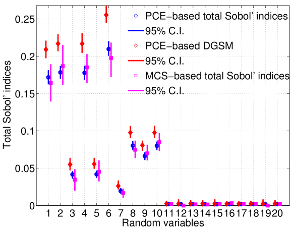
Figure 1: Morris function: PCE-based vs. MCS-based sensitivity measures

For each input variable, Figure 1 depicts the total sensitivity indices computed by MCS and PCE approaches, and the DGSM derived from PCE as well as their corresponding 95% confidence intervals (the bounds of the latter being obtained from the 100 replications). Figure 1 shows that PCE derivative-based sensitivity measures and total Sobol’ indices for parameters $X_{11},\,\dots\,,X_{20}$ are both close to zero, i.e. $X_{11},\,\dots\,,X_{20}$ are unimportant factors. This is consistent with the MCS-based sensitivity measures. Using a sample set of size $500$, the PCE-based approach can detect the non-significant input parameters with acceptable accuracy compared to MCS which requires $110,000$ model runs. In addition, the PCE-based total Sobol’ indices for the remaining parameters vary in a significantly narrower confidence intervals, i.e. are more reliable, than the MCS-based sensitivity indices. Finally, the obtained total Sobol’ indices are always smaller than the DGSMs. The less significant the parameter, the closer DGSM gets to the total Sobol’ index.

5.2 Oakley & O’Hagan function

The second numerical example is the Oakley & O’Hagan function [33, 51] which reads:

$$f(\boldsymbol{X})=\boldsymbol{a}_{1}^{T}\boldsymbol{X}+\boldsymbol{a}_{2}^{T}\cos(\boldsymbol{X})+\boldsymbol{a}_{3}^{T}\sin(\boldsymbol{X})+\boldsymbol{X}^{T}\boldsymbol{M}\boldsymbol{X}$$ (66)

in which the input vector $\boldsymbol{X}=\left\{X_{1},\,\dots\,,X_{15}\right\}$ consists of 15 independent standard normal random variables $\left\{X_{i}\sim{\mathcal{N}}(0,1),\,i=1,\,\dots\,,15\right\}$. The $15\times 1$ vectors $\boldsymbol{a}_{j},\,j=1,2,3$ and the $15\times 15$ matrix $\boldsymbol{M}$ are provided at www.sheffield.ac.uk/st1jeo.

Given the complexity of the function, the PCE-based approach is run with a Latin Hypercube experimental design of size $N=600$. The size of a single sample set for the MCS approach is $N=10,000$ resulting in $10,000\times(2+15)=170,000$ model runs. The procedure is similar as in Section 5.1.

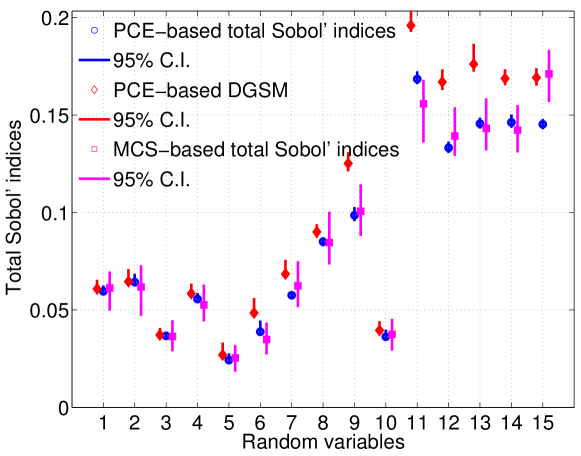
Figure 2: Oakley & O’Hagan function: PCE-based vs. MCS-based sensitivity measures

Figure 2 shows that the PCE-based approach using only $600$ model evaluations can estimate the least significant parameters $X_{3},\,X_{5},\,X_{6},\,X_{10}$ with less uncertainty compared to the MCS approach that uses a huge number of model runs. As already observed in Figure 1, the DGSMs which are the upper bounds of the total Sobol’ indices, are close to the latter for the parameters whose total Sobol’ indices are smaller than 5%. For the remaining parameters which are more influential, the differences between the total Sobol’ indices and their upper bounds become larger.

6 Conclusions

In practical problems, the systems of interest usually contain numerous random input factors which might lead to large uncertainty in the system output and high computational cost. Therefore, it is important to quantify the important and unimportant factors according to their contributions to the output uncertainty. However, the commonly used Monte Carlo simulation (MCS) approach is usually computationally prohibitive.

In this paper, we combined the polynomial chaos expansions (PCE) metamodelling with a derivative-based sensitivity analysis technique. Polynomial chaos expansions are effective surrogate models for global sensitivity analysis. The very nature of the orthogonal expansions reduces the computation of (total) Sobol’ indices to a mere post-processing of the PC coefficients. Similarly, DGSMs can be computed by a straightforward post-processing, i.e. without requiring additional model runs. One only needs to differentiate the multivariate polynomials, which in the end reduces to differentiating univariate polynomial functions. Expressions were given for the classical Hermite, Legendre and Laguerre polynomials. In order to carry out the computation efficiently the derivative polynomials shall be represented onto the orthonormal basis of the same family, which can be do once and for all. Then computing the DGSM reduces to computing weighted sums of the polynomial chaos coefficients. The technique is illustrated on two well-known benchmark functions. By comparing with Monte Carlo simulation, the PCE approach is shown to provide sensitivity indices with smaller uncertainty at a computational cost that is several orders of magnitude smaller.

As seen in Section 4, the computation of polynomial chaos expansions derivative-based global sensitivity measures (PCE-DGSMs) consists of two steps. The first step is to represent the derivative of the PCE in terms of orthonormal polynomials from the same families. It essentially requires to construct the matrices of coefficients $\boldsymbol{C}$ that are used for differentiating the classical orthonormal polynomials. The second step is to post-process this “PCE” of the derivative. A general solution to compute the mean squared derivative using the coefficients matrices $\boldsymbol{C}$ was presented in Section 4.3.

Appendix A Hermite polynomial chaos expansions

The classical Hermite polynomials $\left\{He_{n},n\in{\mathbb{N}}\right\}$, where $n$ determines the degree of the polynomial, are defined on the set of real numbers${\mathbb{R}}$ so as to be orthogonal with respect to the Gaussian probability measure and associated inner product:

$$\langle He_{m},\,He_{n}\rangle\stackrel{{\scriptstyle\text{\tiny def}}}{{=}}\int_{{\mathbb{R}}}He_{m}(z)He_{n}(z)\dfrac{e^{-z^{2}/2}}{\sqrt{2\pi}}\,{\rm d}z=n!\,\delta_{mn}$$ (67)

The Hermite polynomials satisfy the following differential equation [52, Chap. 22]

$$\frac{{\rm d}missing}{{\rm d}z}He_{n}(z)=nHe_{n-1}(z)$$ (68)

From Eq. (67) the norm of Hermite polynomials reads:

$$\langle He_{n},\,He_{n}\rangle=n!$$ (69)

so that the orthonormal Hermite polynomials are defined by:

$$\tilde{He}_{n}(z)=\frac{1}{\sqrt{n!}}He_{n}(z)$$ (70)

Substituting for Eq. (70) in Eq. (68), one gets the derivative of orthonormal Hermite polynomial $\tilde{He}_{n}^{{}^{\prime}}(z)\stackrel{{\scriptstyle\text{\tiny def}}}{{=}}\dfrac{{\rm d}\tilde{He}(z)}{{\rm d}z}$:

$$\tilde{He}_{n}^{{}^{\prime}}(z)=\sqrt{n}\,\tilde{He}_{n-1}(z)$$ (71)

For computational purposes the following matrix notation is introduced:

$$\left\{\tilde{He}_{1}^{{}^{\prime}}(z),\,\dots\,,\tilde{He}_{n}^{{}^{\prime}}(z)\right\}^{\textsf{T}}=\boldsymbol{C}^{{\mathcal{H}}}\cdot\{\tilde{He}_{0}(z),\,\dots\,,\tilde{He}_{n-1}(z)\}^{\textsf{T}}$$ (72)

which allows one to cast the derivative of the orthonormal Hermite polynomials in the initial basis. From Eq. (71), $\boldsymbol{C}^{{\mathcal{H}}}$ is obviously diagonal:

$$\boldsymbol{C}_{i,j}^{{\mathcal{H}}}=\sqrt{i}\,\delta_{ij}$$ (73)

Appendix B Legendre polynomial chaos expansions

The classical Legendre polynomials $\left\{Le_{n},n\in{\mathbb{N}}\right\}$ are defined over $[-1,1]$ so as to be orthogonal with respect to the uniform probability measure and associated inner product:

$$\langle Le_{m},\,Le_{n}\rangle\stackrel{{\scriptstyle\text{\tiny def}}}{{=}}\int_{-1}^{1}Le_{m}(z)Le_{n}(z)\dfrac{{\rm d}z}{2}=\dfrac{1}{2\,n+1}\,\delta_{mn}$$ (74)

They satisfy the following differential equation [52, Chap. 22]

$$\frac{\mathrm{d}}{\mathrm{d}z}\left[Le_{n+1}(z)-Le_{n-1}(z)\right]=(2n+1)Le_{n}(z)$$ (75)

Using the notation ${Le}_{n}^{{}^{\prime}}(z)\stackrel{{\scriptstyle\text{\tiny def}}}{{=}}\dfrac{{\rm d}Le_{n}(z)}{{\rm d}z}$ one can transform Eq. (75) into the equation:

$$Le_{n+1}^{{}^{\prime}}(z) =(2n+1)Le_{n}(z)+Le_{n-1}^{{}^{\prime}}(z)$$ (76)

$$=(2n+1)Le_{n}(z)+(2(n-2)+1)Le_{n-2}(z)+Le_{n-3}^{{}^{\prime}}(z)$$

$$=\cdots$$

From Eq. (74), the norm of Legendre polynomials reads:

$$\langle Le_{n},\,Le_{n}\rangle=\dfrac{1}{2\,n+1}$$ (77)

so that the orthonormal Legendre polynomials read:

$$\tilde{Le}_{n}(z)=\sqrt{2n+1}\,Le_{n}(z)$$ (78)

Substituting for Eq. (78) in Eq. (76) one obtains:

$$\begin{split}\tilde{Le}_{n+1}^{{}^{\prime}}(z)=\sqrt{2n+3}\,&\Big{[}\sqrt{2n+1}\,\tilde{Le}_{n}(z)+\sqrt{2(n-2)+1}\,\tilde{Le}_{n-2}(z)\\ &+\sqrt{2(n-4)+1}\,\tilde{Le}_{n-4}(z)+\dots\Big{]}\end{split}$$ (79)

Introducing the matrix notation:

$$\left\{\tilde{Le}_{1}^{{}^{\prime}}(z),\,\dots\,,\tilde{Le}_{n}^{{}^{\prime}}(z)\right\}^{\textsf{T}}=\boldsymbol{C}^{{\mathcal{L}}e}\cdot\{\tilde{Le}_{0}(z),\,\dots\,,\tilde{Le}_{n-1}(z)\}^{\textsf{T}}$$ (80)

the matrix $\boldsymbol{C}^{{\mathcal{L}}e}$ reads:

$$\boldsymbol{C}^{{\mathcal{L}}e}=\begin{bmatrix}\sqrt{3}&0&0&0&\ldots\\ 0&\sqrt{5}\sqrt{3}&0&0&\ldots\\ \sqrt{7}\cdot 1&0&\sqrt{7}\sqrt{5}&0&\ldots\\ \vdots\\ 0&\sqrt{4p+1}\sqrt{3}&0&\sqrt{4p+1}\sqrt{7}&\ldots&\sqrt{4n+1}\sqrt{4n-1}\\ \end{bmatrix}$$ (81)

when $n=2p$ is even and

$$\boldsymbol{C}^{{\mathcal{L}}e}=\begin{bmatrix}\sqrt{3}&0&0&0&\ldots\\ 0&\sqrt{5}\sqrt{3}&0&0&\ldots\\ \sqrt{7}\cdot 1&0&\sqrt{7}\sqrt{5}&0&\ldots\\ \vdots\\ \sqrt{4p+3}\cdot 1&0&\sqrt{4p+3}\sqrt{5}&0&\ldots&0&\sqrt{4p+3}\sqrt{4p+1}\end{bmatrix}$$ (82)

when $n=2p+1$ is odd.

Appendix C Generalized Laguerre polynomial chaos expansions

Consider a model $Y={\mathcal{M}}(\boldsymbol{X})$ where the input vector $\boldsymbol{X}$ contains $M$ independent random variables with Gamma distribution $X_{i}\sim\Gamma(\alpha_{i},\beta_{i}),\,(\alpha_{i},\beta_{i}>0)$ with prescribed probability density functions:

$$f_{X_{i}}(x_{i})={\beta_{i}}^{\alpha_{i}}\,\dfrac{1}{\Gamma(\alpha_{i})}x^{\alpha_{i}-1}e^{-\beta_{i}x_{i}}$$ (83)

where $\Gamma(\cdot)$ is the Gamma function. We first use an isoprobabilistic transform to convert the input factors into a random vector $\boldsymbol{Z}=\left\{Z_{i},\,\dots\,,Z_{M}\right\}$ as follows:

$$Z_{i}=\beta_{i}\,X_{i}$$ (84)

One can prove that:

$$f_{Z_{i}}(z_{i})=\left|\dfrac{{\rm d}x_{i}}{{\rm d}z_{i}}\right|f_{X_{i}}(x_{i})=\dfrac{1}{\Gamma(\alpha)}{z_{i}}^{\alpha-1}e^{-z_{i}}$$ (85)

which means $Z_{i}\sim\Gamma(\alpha_{i},1)$.

By definition, the generalized Laguerre polynomials $\left\{L_{n}^{(\alpha-1)}(z),\,n\in{\mathbb{N}}\right\}$, where $n$ is the degree of the polynomial, are orthogonal with respect to the weight function $w(z)=z^{\alpha-1}e^{-z}$ over $(0,\infty)$:

$$\langle L_{n}^{(\alpha-1)}(z),L_{m}^{(\alpha-1)}(z)\rangle\stackrel{{\scriptstyle\text{\tiny def}}}{{=}}\int\limits_{0}^{+\infty}z^{\alpha-1}e^{-z}L_{n}^{(\alpha-1)}(z)L_{m}^{(\alpha-1)}(z){\rm d}z=\dfrac{\Gamma(n+\alpha)}{n!}\delta_{mn}$$ (86)

The derivative of $L_{n}^{(\alpha-1)}$ reads:

$$L_{n}^{{}^{\prime}(\alpha-1)}(z)=-\sum_{k=0}^{n-1}L_{k}^{(\alpha-1)}(z)$$ (87)

Recall that one obtains the Gamma distribution by scaling the weight function $w(z)$ by $1/\Gamma(\alpha)$. Therefore in the context of PCE, we use the generalized Laguerre polynomials functions orthonormalized as follows:

$$\tilde{L}_{n}^{(\alpha-1)}(z)=\sqrt{\dfrac{n!\Gamma(\alpha)}{\Gamma(n+\alpha)}}L_{n}^{(\alpha-1)}(z)=\sqrt{n\,B(n,\alpha)}\,L_{n}^{(\alpha-1)}(z)$$ (88)

where $B(x,y)=\frac{\Gamma(x)\Gamma(y)}{\Gamma(x+y)}$ is the beta function. Substituting for Eq. (88) in Eq. (87) one obtains:

$$\tilde{L}_{n}^{{}^{\prime}(\alpha-1)}(z)=-\sum_{k=0}^{n-1}\sqrt{\dfrac{\Gamma(k+\alpha+1)\,n!}{\Gamma(n+\alpha+1)\,k!}}\tilde{L}_{k}^{(\alpha-1)}(z)=-\sum_{k=1}^{n}\sqrt{\frac{B(n+1,\alpha)}{B(k,\alpha)}}\tilde{L}_{k-1}^{(\alpha-1)}(z)$$ (89)

Introducing the matrix notation:

$$\left\{\tilde{L}_{1}^{{}^{\prime}}(z),\,\dots\,,\tilde{L}_{n}^{{}^{\prime}}(z)\right\}^{\textsf{T}}=\boldsymbol{C}^{{\mathcal{L}}a}\cdot\{\tilde{L}_{0}(z),\,\dots\,,\tilde{L}_{n-1}(z)\}^{\textsf{T}}$$ (90)

the constant matrix $\boldsymbol{C}^{{\mathcal{L}}a}$ is a lower triangular matrix whose generic term reads:

$$\boldsymbol{C}_{i,j}^{{\mathcal{L}}a}=-\sqrt{\frac{B(i+1,\alpha)}{B(j,\alpha)}}$$ (91)

References

• Reuter and Liebscher [2008] Reuter, U., Liebscher, M.. Global sensitivity analysis in view of nonlinear structural behavior. LSDYNA Anwenderforum, Bamberg 2008;.
• Hasofer [2009] Hasofer, A.M.. Modern sensitivity analysis of the CESARE-Risk computer fire model. Fire Safety J 2009;44(3):330–338.
• Campolongo et al. [2007] Campolongo, F., Cariboni, J., Saltelli, A.. An effective screening design for sensitivity analysis of large models. Environmental modelling & software 2007;22(10):1509–1518.
• Sudret et al. [2013] Sudret, B., Mai, C.V., Mai, V.C.. Computing seismic fragility curves using polynomial chaos expansions. In: Deodatis, G., editor. Proc. 11th Int. Conf. Struct. Safety and Reliability (ICOSSAR’2013), New York, USA. 2013,.
• Patelli and Pradlwarter [2010] Patelli, E., Pradlwarter, H.J.. Monte Carlo gradient estimation in high dimensions. Int J Numer Meth Engng 2010;81(2):172–188.
• Sudret [2007] Sudret, B.. Uncertainty propagation and sensitivity analysis in mechanical models - Contributions to structural reliability and stochastic spectral methods. Ph.D. thesis; Université BLAISE PASCAL - Clermont II; 2007.
• de Rocquigny [2012] de Rocquigny, E.. Modelling Under Risk and Uncertainty. Wiley Series in Probability and Statistics; Chichester, UK: John Wiley & Sons, Ltd; 2012.
• Saltelli et al. [2000] Saltelli, A., Chan, K., Scott, E.. Sensitivity analysis. J. Wiley & Sons; 2000.
• Saltelli et al. [2004] Saltelli, A., Tarantola, S., Campolongo, F., Ratto, M.. Sensitivity analysis in practice: a guide to assessing scientific models. J. Wiley & Sons; 2004.
• Saltelli et al. [2008] Saltelli, A., Ratto, M., Andres, T., Campolongo, F., Cariboni, J., Gatelli, D., et al. Global Sensitivity Analysis – The Primer. Wiley; 2008.
• Pappenberger et al. [2008] Pappenberger, F., Beven, K.J., Ratto, M., Matgen, P.. Multi-method global sensitivity analysis of flood inundation models. Adv Water Resour 2008;31(1):1–14.
• Kala [2011] Kala, Z.. Sensitivity analysis of steel plane frames with initial imperfections. Eng Struct 2011;33(8):2342–2349.
• Fassò [2013] Fassò, A.. Sensitivity Analysis of Computer Models. John Wiley & Sons, Ltd; 2013,.
• Borgonovo and Peccati [2006] Borgonovo, E., Peccati, L.. Uncertainty and global sensitivity analysis in the evaluation of investment projects. Int J Prod Econ 2006;104(1):62–73.
• Marino et al. [2008] Marino, S., Hogue, I.B., Ray, C.J., Kirschner, D.E.. A methodology for performing global uncertainty and sensitivity analysis in systems biology. J Theor Biol 2008;254(1):178–196.
• Abraham et al. [2007] Abraham, A.K., Krzyzanski, W., Mager, D.E.. Partial derivative-based sensitivity analysis of models describing target-mediated drug disposition. The AAPS journal 2007;9(2):E181–E189.
• Kucherenko et al. [2009] Kucherenko, S., Rodriguez-Fernandez, M., Pantelides, C., Shah, N.. Monte Carlo evaluation of derivative-based global sensitivity measures. Reliab Eng Sys Safety 2009;94(7):1135–1148.
• Morris [1991] Morris, M.D.. Factorial Sampling Plans for Preliminary Copmputational Experiments. Technometrics 1991;33(2):161–174.
• Cukier et al. [1973] Cukier, R.I., Fortuin, C.M., Shuler, K.E., Petschek, A.G., Schaibly, J.H.. Study of the sensitivity of coupled reaction systems to uncertainties in rate coefficients - theory. J Chem Phys 1973;59:38,73–3878.
• Cukier et al. [1978] Cukier, H., Levine, R.I., Shuler, K.. Nonlinear sensitivity analysis of multiparameter model systems. J Comput Phys 1978;26:1–42.
• Mara [2009] Mara, T.A.. Extension of the RBD-FAST method to the computation of global sensitivity indices. Reliab Eng Sys Safety 2009;94(8):1274–1281.
• Sobol’ [1993] Sobol’, I.M.. Sensitivity estimates for nonlinear mathematical models. Math Modeling & Comp Exp 1993;1:407–414.
• Sobol′ [2001] Sobol′, I.. Global sensitivity indices for nonlinear mathematical models and their Monte Carlo estimates. Mathematics and Computers in Simulation 2001;55(1-3):271–280.
• Sobol’ and Kucherenko [2005] Sobol’, I.M., Kucherenko, S.S.. Global sensitivity indices for nonlinear mathematical models. Review. Wilmott magazine 2005;1:56–61.
• Archer et al. [1997] Archer, G.E., Saltelli, A., Sobol’, I.M.. Sensitivity measures, ANOVA-like techniques and the use of bootstrap. J Stat Comput Simul 1997;58:99–120.
• Saltelli [2002] Saltelli, A.. Making best use of model evaluations to compute sensitivity indices. Comput Phys Comm 2002;145:280–297.
• Saltelli et al. [2010] Saltelli, A., Annoni, P., Azzini, V., Campolongo, F., Ratto, M., Tarantola, S.. Variance based sensitivity analysis of model output. Design and estimator for the total sensitivity index. Comput Phys Comm 2010;181:259–270.
• Sathyanarayanamurthy and Chinnam [2009] Sathyanarayanamurthy, H., Chinnam, R.B.. Metamodels for variable importance decomposition with applications to probabilistic engineering design. Comput Ind Eng 2009;57(3):996–1007.
• Zhang and Pandey [2014] Zhang, X., Pandey, M.D.. An effective approximation for variance-based global sensitivity analysis. Reliab Eng Sys Safety 2014;121(0):164–174.
• Sudret [2006] Sudret, B.. Global sensitivity analysis using polynomial chaos expansions. In: Spanos, P., Deodatis, G., editors. Proc. 5th Int. Conf. on Comp. Stoch. Mech (CSM5), Rhodos, Greece. 2006,.
• Sudret [2008] Sudret, B.. Global sensitivity analysis using polynomial chaos expansions. Reliab Eng Sys Safety 2008;93:964–979.
• Blatman and Sudret [2010a] Blatman, G., Sudret, B.. Efficient computation of global sensitivity indices using sparse polynomial chaos expansions. Reliab Eng Sys Saf 2010a;95(11):1216–1229.
• Sobol’ and Kucherenko [2009] Sobol’, I.M., Kucherenko, S.. Derivative based global sensitivity measures and their link with global sensitivity indices. Math Comput Simul 2009;79(10):3009–3017.
• Sobol’ and Kucherenko [2010] Sobol’, I.M., Kucherenko, S.. A new derivative based importance criterion for groups of variables and its link with the global sensitivity index. Comput Phys Comm 2010;181(7):1212–1217.
• Lamboni et al. [2013] Lamboni, M., Iooss, B., Popelin, A.L., Gamboa, F.. Derivative-based global sensitivity measures: general links with Sobol’ indices and numerical tests. Math Comput Simul 2013;87:44–54.
• Sobol’ et al. [2007] Sobol’, I.M., Tarantola, S., Gatelli, D., Kucherenko, S., Mauntz, W.. Estimating the approximation error when fixing unessential factors in global sensitivity analysis. Reliab Eng Sys Safety 2007;92(7):957–960.
• Monod et al. [2006] Monod, H., Naud, C., Makowski, D.. Uncertainty and sensitivity analysis for crop models. Working with Dynamic Crop Models: Evaluation, Analysis, Parameterization, and Applications, Elsevier 2006;:55–100.
• Janon et al. [2013] Janon, A., Klein, T., Lagnoux, A., Nodet, M., Prieur, C.. Asymptotic normality and efficiency of two Sobol index estimators. ESAIM: Probability and Statistics 2013;:1–20.
• Ghanem and Spanos [2003] Ghanem, R., Spanos, P.. Stochastic Finite Elements : A Spectral Approach. Courier Dover Publications; 2003.
• Soize and Ghanem [2004] Soize, C., Ghanem, R.. Physical systems with random uncertainties: chaos representations with arbitrary probability measure. SIAM J Sci Comput 2004;26(2):395–410.
• Le Maître et al. [2002] Le Maître, O.P., Reagan, M., Najm, H.N., Ghanem, R.G., Knio, O.M.. A stochastic projection method for fluid flow – II. Random process. J Comput Phys 2002;181:9–44.
• Matthies and Keese [2005] Matthies, H.G., Keese, A.. Galerkin methods for linear and nonlinear elliptic stochastic partial differential equations. Comput Methods Appl Mech Engrg 2005;194:1295–1331.
• Xiu [2009] Xiu, D.. Fast numerical methods for stochastic computations: a review. Comm Comput Phys 2009;5(2-4):242–272.
• Berveiller et al. [2004] Berveiller, M., Sudret, B., Lemaire, M.. Presentation of two methods for computing the response coefficients in stochastic finite element analysis. In: Proc. 9th ASCE Specialty Conference on Probabilistic Mechanics and Structural Reliability, Albuquerque, USA. 2004,.
• Berveiller et al. [2006] Berveiller, M., Sudret, B., Lemaire, M.. Stochastic finite elements: a non intrusive approach by regression. Eur J Comput Mech 2006;15(1-3):81–92.
• Blatman [2009] Blatman, G.. Adaptive sparse polynomial chaos expansions for uncertainty propagation and sensitivity analysis. Ph.D. thesis; Université Blaise Pascal, Clermont-Ferrand; 2009.
• Blatman and Sudret [2010b] Blatman, G., Sudret, B.. An adaptive algorithm to build up sparse polynomial chaos expansions for stochastic finite element analysis. Prob Eng Mech 2010b;25(2):183–197.
• Blatman and Sudret [2011] Blatman, G., Sudret, B.. Adaptive sparse polynomial chaos expansion based on Least Angle Regression. J Comput Phys 2011;230:2345–2367.
• Xiu and Karniadakis [2002] Xiu, D., Karniadakis, G.E.. The Wiener-Askey polynomial chaos for stochastic differential equations. SIAM J Sci Comput 2002;24(2):619–644.
• Pujol et al. [2013] Pujol, G., Iooss, B., Janon, A.. sensitivity: Sensitivity Analysis; 2013.
• Oakley and O’Hagan [2004] Oakley, J., O’Hagan, A.. Probabilistic sensitivity analysis of complex models: a Bayesian approach. J Royal Stat Soc, Series B 2004;66:751–769.
• Abramovitz and Stegun [1965] Abramovitz, M., Stegun, I.A.. Handbook of mathematical functions. New York: Dover Publications Inc.; 1965.