Constraining black hole masses in low-accreting AGN using X-ray spectra

Abstract

In a recent work we demonstrated that a novel X-ray scaling method, originally introduced for Galactic black holes (GBHs), can be reliably extended to estimate the mass of supermassive black holes accreting at a moderate to high level. Here we investigate the limits of applicability of this method to low-accreting active galactic nuclei, using a control sample with good-quality X-ray data and dynamically measured mass. For low-accreting AGNs ($L_{\rm X}/L_{\rm Edd}\leq 10^{-4}$), because the basic assumption that the photon index positively correlates with the accretion rate no longer holds the X-ray scaling method cannot be used. Nevertheless, the inverse correlation in the $\Gamma-L_{\rm X}/L_{\mathrm{Edd}}$ diagram, found in several low-accreting BHs and confirmed by this sample, can be used to constrain $M_{\rm BH}$ within a factor of $\sim 10$ from the dynamically determined values. We provide a simple recipe to determine $M_{\rm BH}$ using solely X-ray spectral data, which can be used as a sanity check for $M_{\rm BH}$ determination based on indirect optical methods.

1 Introduction

It is now widely accepted that black holes exist on very different scales, with masses that range between 3–20 $M_{\odot}$ for stellar mass black holes (sMBHs) and $10^{6}-10^{9}~{}M_{\odot}$ for supermassive black holes (SMBHs) at the center of galaxies and in active galactic nuclei (AGNs), with possibly intermediate black holes ($M_{\rm BH}=10^{2}-10^{5}~{}M_{\odot}$) whose nature is still a matter of debate.

Recent studies have provided evidence for the presence of supermassive black holes at the center of virtually every galaxy with a prominent bulge and for the existence of tight correlations between $M_{\rm BH}$ and several galaxy parameters such as the velocity dispersion or the mass of the bulge (Magorrian et al., 1998; Gebhardt et al., 2000a; Ferrarese & Merritt, 2000). This bolsters the importance and ubiquity of these systems in the universe and suggests that black hole and galaxy growth may be closely related and that black holes are essential ingredients in the evolution of galaxies.

Black holes are fairly simple objects that are completely described by only three parameters, mass, spin, and charge, with the latter generally negligible in astrophysical studies. However, since active BHs are not isolated systems but feed on the gas provided by a stellar companion or on the gas accumulated at the center of galaxies, the dimensionless accretion rate $\dot{m}$ (defined as $\dot{m}=L_{\rm bol}/L_{\rm Edd}$, where $L_{\rm bol}$ is the bolometric luminosity and $L_{\rm Edd}=1.3\times 10^{38}\,M_{\rm BH}/M_{\odot}$ erg s^-1 the Eddington luminosity) in Eddington units should be counted as an additional basic parameter.

The determination of $M_{\rm BH}$ is one of the most crucial tasks to shed light on accretion and ejection phenomena in both supermassive and stellar BHs, because $M_{\rm BH}$ sets the time and length scales in these systems, and may play a fundamental role in the formation and evolution of galaxies. The most direct way to determine $M_{\rm BH}$ is via dynamical methods. Under the assumption of Keplerian motion, a lower limit on the mass of the compact object can be determined in GBHs by measuring orbital period and velocity of the visible stellar companion. Similarly, in nearby weakly active or quiescent galaxies the estimate of $M_{\rm BH}$ can be inferred by directly modeling the dynamics of gas or stars in the vicinity of the black hole (e.g., Kormendy & Richstone 1995; Magorrian et al. 1998). For highly active galaxies that show significant optical variability, the estimate of $M_{\rm BH}$ relies upon the so-called “reverberation mapping” method, where the “test particles” are represented by high-velocity gas clouds, whose dynamics are dominated by the BH gravitational force and are usually referred to as the broad-line region (BLR), since their radiation is dominated by broad emission lines (Peterson, 1993).

These direct methods are the most accurate and reliable ways to constrain $M_{\rm BH}$, but at the same time have severe limitations: the methods applied to semi-quiescent galaxies require the sphere of influence of the black hole to be resolved by the instruments, and hence can be extended only to nearby objects. On the other hand, the reverberation mapping technique requires significant resources and time, and cannot be applied to very luminous sources, whose variability is typically characterized by small-amplitude flux changes occurring on very long timescales, or to sources without a detected BLR. In order to circumvent these limitations, several secondary indirect methods have been developed (see, e.g., Vestergaard, 2009). Most of them rely on some empirical relationship between $M_{\rm BH}$ and different properties of the host galaxy or are based on results obtained from the reverberation mapping such as the radius-luminosity relationship (Kaspi et al., 2000). However, the extension of these empirical relationships to systems with $M_{\rm BH}$ and $\dot{m}$ vastly different from the original limited samples is still untested, and the majority of these techniques still requires a detected BLR, significantly restricting the number of possible AGNs and the black hole mass range that can be studied.

In order to perform statistical studies of BHs and understand their evolutionary history and connection to their host galaxies, it is important to explore alternative ways to determine the BH mass that are not dependent on the assumptions of optical-based methods. An important role in this field may be played by X-ray-based methods, since the X-rays are nearly ubiquitous in accreting BH systems regardless of their mass or accretion state, are less affected by absorption than optical/UV emission, and are produced and reprocessed in the vicinity of the BH thus closely tracking its activity.

Recently, Shaposhnikov & Titarchuk (2009) developed a new X-ray scaling method to determine $M_{\rm BH}$ for GBHs. This method is based on the positive correlation between X-ray photon index $\Gamma$ (which is generally considered as a reliable indicator of the accretion state of the source; see e.g., Shemmer et al. (2007, 2008); Esh et al. (1997)) and the source brightness, parameterized by the normalization of the Bulk Motion Comptonization (BMC) model. The self-similarity of this spectral trend, which is observed in different GBHs during different outbursts events, makes it possible to estimate $M_{\rm BH}$ in any GBHs by scaling the dynamically-constrained value of $M_{\rm BH}$ of a GBH considered as a reference source.

With the assumption that AGNs follow the same spectral evolution as GBHs (although on much longer timescales that cannot be directly probed), in our recent work, we tested whether this novel X-ray scaling method could be extended to supermassive BHs. To this end, we utilized a sample of AGNs with good X-ray data and whose BH mass had been already determined via reverberation mapping. The results (on average the $M_{\rm BH}$ values determined with this method are within a factor of 2-3 from the reverberation mapping values) demonstrate that this method is reliable and robust for BH systems accreting at moderate and high rate ($\dot{m}\geq$ 1%) and can be used to determine BH masses at any scale (Gliozzi et al., 2011).

The presence of a positive correlation between $\Gamma$ and $L_{\mathrm{X}}$ (which is at the basis of the X-ray scaling method) has been observed in highly and moderately accreting BH systems at all scales for several decades. For example, a spectral steepening as the source brightens is consistently observed in the evolution between canonical spectral states in GBHs (e.g., Esin et al. 1997; Homan et al. 2001, and references therein). A similar behavior has been also observed in individual and samples of AGNs (e.g., Markowitz & Edelson 2001; Papadakis et al. 2002; Shemmer et al. 2008). On the other hand, in the very low accreting regime ($\dot{m}\ll 1\%$) convincing evidence of a $\Gamma$ $-$ $L_{\mathrm{X}}$ (or $L_{X}/L_{\mathrm{Edd}}$) anti-correlation has been revealed only recently (e.g., Wu & Gu 2008; Constantin et al. 2009; Gu & Cao 2009; Younes et al. 2011; G$\mathrm{\ddot{u}}$ltekin et al. 2012; see however Trump et al. 2011 for an alternative view).

Here, we want to investigate the limits of applicability of this method to low-accreting BH systems, by applying it to a sample of low-accreting AGNs, which possess good-quality X-ray data (either from Chandra or XMM-Newton satellites) and with $M_{\rm BH}$ determined from direct dynamical methods. In principle, since the direct $\Gamma$ $-$ $L_{\mathrm{X}}$ correlation is the foundation of the scaling method and since at very low accreting levels no positive correlation is observed, it is expected that at a certain threshold value of $\dot{m}$ the X-ray scaling method should break down. Nevertheless, it is important to test if this break down actually occurs (this would provide indirect support to the foundation of the method, i.e., the self-similar spectral behavior of BHs at all scales) and at which value of $\dot{m}$ does it occur.

The description of the sample and the data reduction are provided in Section 2 and 3, respectively. The X-ray spectral analysis is performed in Section 4. In Section 5, we apply the X-ray scaling method and show that the overall spectral behavior of our sample is consistent with an anti-correlation in the $\Gamma-L_{X}/L_{\rm Edd}$ plot, which provides an alternative way to constrain $M_{\rm BH}$. The main results and their implications are summarized and discussed in Section 6.

2 Description of the sample

In order to test X-ray-based methods to determine $M_{\rm BH}$ in low-accreting AGNs, we need to select objects that fulfill the following criteria: 1) they must have a direct and robust estimate of $M_{\rm BH}$; 2) they must possess good-quality X-ray data; and 3) they must accrete at low level, $L_{X}/L_{\mathrm{Edd}}$ $\ll 1$%.

Our sample contains a total of 53 low-luminosity AGNs (LLAGNs) with bolometric luminosity less than $10^{42}$ erg s^-1 (Ho et al. 2001) and whose black hole mass has been determined via dynamical methods. The physical properties of the sources are listed in Table 1, in which column (1) provides the source name, columns (2) and (3) right ascension and declination, (4) the $M_{\rm BH}$ value via the dynamical method, (5) the redshift-independent distance from the NSAS/IPAC Extragalactic Database (NED), (6) the $H_{\alpha}/H_{\beta}$ ratio, (7) the flux of the narrow component of [OIII]$\lambda 5007$, (8) the radio luminosity, (9) the AGN class (S=Seyfert galaxies, L=LINERs), and (10) the galaxy class. The narrow-line emission and types were gathered from the Palomar survey (Ho et al., 1997) unless stated otherwise. Based on the optical classification, this sample comprises 16 LINERs, 17 Seyfert galaxies ranging from type 1 to type 2, and 20 AGNs that are not optically classified.

Table 1: The sample of LLAGNs. Optical and radio properties

Source Name	RA	DEC	$\log(M_{BH}/M_{\odot})$	D (Mpc)	Hα/Hβ	$\log(F_{[\rm OIII]})$	$\log(L_{\rm 6cm})$	AGN Class	Optical Class
(1)	(2)	(3)	(4)	(5)	(6)	(7)	(8)	(9)	(10)
IC 1459	22 : 57 : 10.6	-36 : 27 : 44	$9.44\pm 0.20^{1}$	29.2			39.76	L/R	E3 f
IC 4296	13 : 36 : 39.0	-33 : 57 : 57	$9.13\pm 0.07^{2}$	62.2			38.59	L	E1 g
NGC 221	00 : 42 : 41.8	40 : 51 : 55	$6.49\pm 0.09^{3}$	0.81			33.3		E2
NGC 224	00 : 42 : 44.3	41 : 16 : 09	$8.17\pm 0.16^{4}$	0.84			32.14	L	SA(s)b
NGC 821	02 : 08 : 21.1	10 : 59 : 42	$7.63\pm 0.16^{5}$	22.4					E6
NGC 1023	02 : 40 : 24.0	39 : 03 : 48	$7.66\pm 0.04^{6}$	9.82					SB(rs)0-
NGC 1068	02 : 42 : 40.7	00 : 00 : 48	$6.93\pm 0.02^{7}$	10.1	5.29	-10.46	39.18	S2	(r)SA(rs)b
NGC 1300	03 : 19 : 41.1	-19 : 24 : 41	$7.85\pm 0.29^{8}$	22.6					SB(rs)bc
NGC 1399	03 : 38 : 29.1	-35 : 27 : 03	$8.71\pm 0.06^{9}$	19.4				S2 b	E1
NGC 2748	09 : 13 : 43.0	76 : 28 : 31	$7.67\pm 0.50^{8}$	21.0	6.11	-15.00		H	Sabc
NGC 2778	09 : 12 : 24.4	35 : 01 : 39	$7.21\pm 0.32^{5}$	38.1					E2
NGC 2787	09 : 19 : 18.6	69 : 12 : 12	$7.64\pm 0.05^{10}$	7.48	1.89	-13.93	37.22	L	SB(r)0+
NGC 3031	09 : 55 : 33.2	69 : 03 : 55	$7.90\pm 0.09^{11}$	3.65	3.15	-12.65	36.82	L b	SA(s)ab
NGC 3115	10 : 05 : 14.0	-07 : 43 : 07	$8.98\pm 0.18^{12}$	9.68				S	SA0- sping
NGC 3227	10 : 23 : 30.6	19 : 51 : 54	$7.18\pm 0.23^{13}$	21.1	2.9	-12.02	37.72	S1.5	SAB(s)a pec
NGC 3245	10 : 27 : 18.4	28 : 30 : 27	$8.35\pm 0.11^{14}$	27.4	4.76	-13.42	36.98	L	SA(r)0?
NGC 3377	10 : 47 : 42.3	13 : 59 : 09	$8.06\pm 0.16^{5}$	11.3		-10.20 c			E5+
NGC 3379	10 : 47 : 49.6	12 : 34 : 54	$8.09\pm 0.25^{15}$	12.6		-14.16		L	E1
NGC 3384	10 : 48 : 16.9	12 : 37 : 45	$7.25\pm 0.04^{5}$	10.8		-10.60 c			SB(s)0-
NGC 3585	11 : 13 : 17.1	-26 : 45 : 17	$8.53\pm 0.12^{16}$	20.2					S0
NGC 3607	11 : 16 : 54.6	18 : 03 : 06	$8.08\pm 0.15^{16}$	22.8	5.56	-13.26		S2 b	SA(s)0:
NGC 3608	11 : 16 : 58.9	18 : 08 : 55	$8.32\pm 0.17^{5}$	23.1		-14.16		L	E2
NGC 3998	11 : 57 : 56.1	55 : 27 : 13	$8.37\pm 0.43^{17}$	19.4	4.72	-13.13	38.03	L b	SA(r)0?
NGC 4026	11 : 59 : 25.2	50 : 57 : 42	$8.33\pm 0.11^{16}$	11.7	3.4	-10.95			(R’)SAB(rs)ab:
NGC 4151	12 : 19 : 23.2	05 : 49 : 31	$7.65\pm 0.05^{18}$	3.89			38.2	S1.5	SA0 spin
NGC 4258	12 : 18 : 57.5	47 : 18 : 14	$7.58\pm 0.00^{19}$	7.59	3.94	-12.98	36.03	S1.9	SAB(s)bc
NGC 4261	12 : 19 : 23.2	05 : 49 : 31	$8.74\pm 0.09^{20}$	24.0	4.9	-13.43	39.21	L	E2+
NGC 4278	12 : 20 : 06.8	29 : 16 : 51	$9.20\pm 0.00^{21}$	10.0	2.5	-13.17	37.91	L	E1+
NGC 4291	12 : 20 : 18.2	75 : 22 : 15	$8.51\pm 0.34^{5}$	31.2					E
NGC 4303	12 : 21 : 54.9	04 : 28 : 25	$6.65\pm 0.35^{22}$	12.2	3.92	-12.97	38.46	S2 b	SAB(rs)bc
NGC 4342	12 : 23 : 39.0	07 : 03 : 14	$8.56\pm 0.19^{23}$	16.8					S0
NGC 4374	12 : 25 : 03.7	12 : 25 : 04	$9.18\pm 0.23^{24}$	17.5	4.68	-13.46	38.77	S2	E1
NGC 4395	12 : 25 : 48.8	33 : 32 : 49	$5.04\pm 0.00^{25}$	4.83	2.13	-12.46	35.56	S1.8	SA(s)m:
NGC 4459	12 : 29 : 00.0	13 : 58 : 42	$7.87\pm 0.08^{10}$	16.6	3.24	-14.64		L	SA(r)0+
NGC 4473	12 : 29 : 48.9	13 : 25 : 46	$8.11\pm 0.35^{5}$	15.2					E5
NGC 4486	12 : 30 : 49.4	12 : 23 : 28	$9.56\pm 0.13^{26}$	15.9	4.29	-12.97	39.83	L	E0+pec
NGC 4486A	12 : 30 : 57.7	12 : 16 : 13	$7.13\pm 0.15^{27}$	15.1				E2
NGC 4564	12 : 36 : 27.0	11 : 26 : 21	$7.84\pm 0.05^{5}$	15.8					E
NGC 4594	12 : 39 : 59.4	-11 : 37 : 23	$8.76\pm 0.41^{28}$	13.7	3.37	-12.46 a	37.89	Sy1.9 b	SA(s)a spin
NGC 4596	12 : 39 : 55.9	10 : 10 : 34	$7.92\pm 0.16^{11}$	16.8	2.12	-15.35		L	SB(r)0+
NGC 4649	12 : 43 : 40.0	11 : 33 : 10	$9.33\pm 0.12^{5}$	14.0			37.45		E2
NGC 4697	12 : 48 : 35.9	-05 : 48 : 03	$8.29\pm 0.04^{5}$	20.9		-15.90 d			E6
NGC 4742	12 : 51 : 48.0	-10 : 27 : 17	$7.18\pm 0.15^{29}$	15.5					E h
NGC 4945	13 : 05 : 27.5	-49 : 28 : 06	$6.15\pm 0.18^{30}$	4.50			38.17	S b
NGC 5077	13 : 19 : 31.7	-12 : 39 : 25	$8.90\pm 0.22^{31}$	39.8	2.89	-13.82		L	E3+

• $M_{\rm BH}$ Reference: (1) Cappellari et al. 2002; (2) Dalla Bont$\grave{\rm a}$ et al. 2009; (3) Verolme et al. 2002; (4) Bender et al. 2005; (5) Gebhardt et al. 2000a; (6) Bower et al. 2001; (7) Lodato & Bertin 2003; (8) Atkinson et al. 2005; (9) Gebhardt et al. 2007; (10) Sarzi et al. 2001; (11) Devereux et al. 2003; (12) Emsellem et al. 1999; (13) Hicks et al. 2008; (14) Barth et al. 2001; (15) Gebhardt et al. 2000b; (16) G$\ddot{\rm u}$ltekin et al. 2009a; (17) de Francesco et al. 2006; (18) Onken et al. 2007; (19) Herrnstein et al. 2005; (20) Ferrarese et al. 1996; (21) Cardullo et al. 2009; (22) Pastorini et al. 2007; (23) Cretton & van den Bosch 1999; (24) Bower et al. 1998; (25) Haim et al. 2012; (26) Macchetto et al. 1997; (27) Nowak et al. 2007; (28) Kormendy 1988; (29) listed as M. E. Kaiser et al. 2002 in preparation in Tremaine et al. 2002 but never published; (30) Greenhill et al. 1997; (31) de Francesco et al. 2008; (32) Silge et al. 2005; (33) Capetti et al. 2005; (34) Ferrarese & Ford 1999; (35) van der Marel & van den Bosch 1998; (36) Wold et al. 2006
  

Table 1 Continued $-$ The sample of LLAGNs. Optical and radio properties

Source Name	RA	DEC	$\log(M_{BH}/M_{\odot})$	z	Hα/Hβ	$\log(F_{[\rm OIII]})$	$\log(L_{\rm 6cm})$	AGN Class	Optical Class
NGC 5128	13 : 25 : 27.6	-43 : 01 : 09	$8.48\pm 0.04^{32}$	4.09	3.72 a	-13.15 e	39.85	S2
NGC 5252	13 : 38 : 15.9	04 : 32 : 33	$9.00\pm 0.34^{33}$	99.3	3.72 a	-12.41	39.05	S2 b	S0
NGC 5576	14 : 21 : 03.7	03 : 16 : 16	$8.26\pm 0.09^{16}$	25.8					E3
NGC 5845	15 : 06 : 0.80	01 : 38 : 02	$8.46\pm 0.22^{5}$	24.1					E3
NGC 6251	16 : 32 : 32.0	82 : 32 : 16	$8.78\pm 0.15^{37}$	97.6	15.1 a	-11.90	41.01	S2	E1
NGC 7052	21 : 18 : 33.0	26 : 26 : 49	$8.60\pm 0.22^{38}$	56.7			39.43		E3
NGC 7457	23 : 00 : 59.9	30 : 08 : 42	$6.61\pm 0.17^{5}$	12.3		-16.18		S	SA(rs)0-?
NGC 7582	23 : 18 : 23.5	-42 : 22 : 14	$7.74\pm 0.10^{39}$	22.2	7.6 a	-11.35	38.55	S2 b	Sbab

• Note $-$ AGN Class $-$ S: Seyfert Galaxies, L: LINERs
  ^a Bassani et al. 1999; ^bVéron-Cetty & Véron 2006; ^cCiardullo et al. 1989; ^d Méndez et al. 2005; ^e Walsh et al. 2012; ^f Fabbiano et al. 2003; ^gYounis et al. 1985; ^h Naim et al. 1995

The dynamical mass measurements are based on high spatial resolution stellar velocity measurements (Ghez et al., 2008; G$\mathrm{\ddot{u}}$ltekin et al., 2009b), gas dynamic measurements (Barth et al., 2001), and maser measurements (Miyoshi et al., 1995). All sources have been observed with Chandra and most have also XMM-Newton data. Chandra with its unsurpassed spatial resolution is ideal to disentangle the different X-ray components, whereas XMM-Newton with its large collecting area and consequent higher sensitivity provides tighter constraints on the X-ray spectral parameters for isolated point-like sources.

3 Data reduction

3.1 Chandra observations

In the Chandra archive, for each source we selected the observations with the longest exposures and the smallest pointing offset with respect to the nominal position of the AGN. Most of the observations are the same as those analyzed by G$\mathrm{\ddot{u}}$ltekin et al. (2009b). Adding six new sources observed more recently by G$\mathrm{\ddot{u}}$ltekin et al. (2012) and 2 described by Gu & Cao (2009), the total number of sources with Chandra data is 53.

The data reduction was carried out homogeneously for each source as described below. Source’s spectra and light curves were extracted from circular regions with a radius of $1"-2"$, and their background from nearby source-free circular regions with a radius of $10"-20"$. Sometimes, extraction regions were extended to $\sim 3"$ for brighter sources. The data reduction followed the standard pipeline, using Chandra data reduction software package version CIAO 4.4, and the nuclear source regions were confirmed after running wavdetect (Freeman et al., 2002). Background flares were cut above $3\sigma$ from the mean value. The positions of source and background were given as input to the specextract tool to create the response matrix file (RMF) and ancillary response file (ARF).

3.2 XMM-Newton Observations

36 sources (nearly 70% of the Chandra sample) also possess XMM-Newton data. We performed the data reduction following the standard procedures of Science Analysis System (SAS) version 12.0.1. We only selected good X-ray event (“FLAG=0”) with patterns $0-4$ and $0-12$ for pn and MOS, respectively. The positions inferred from Chandra were used as center of the extraction regions with a radius of $\sim 10"$ or larger for brighter and extended sources. When the nuclear source was located at the edge of a CCD or between two CCDs, we utilized the second longest XMM-Newton observation. The background regions were chosen in nearby empty spaces on the same CCD for both pn and MOS cameras. We used Chandra images and spectra to account for the presence of additional X-ray components (e.g., diffuse emission, jet-like structures, off-nuclear sources) in the XMM-Newton extraction regions. The SAS rmfgen and argen task were used to generate RMF and ARF files, respectively. Of the 36 sources observed at least once by XMM-Newton, 33 of them have sufficient statistics for a meaningful spectral analysis.

3.3 Image Inspection

Since the Point Spread Function (PSF) of XMM-Newton EPIC cameras does not allow one to firmly distinguish between point-like and extended emission in low-luminosity sources, a systematic comparison of XMM-Newton and Chandra images was done to investigate the presence of additional X-ray components in the extraction region.

To this end, we overlapped Chandra image contours on the corresponding XMM-Newton images. From the Chandra images, we also measured source counts using different extraction regions (with radii of $10"$ and $20"$), in order to estimate the contribution of off-nuclear components encompassed by the larger extraction region of XMM-Newton.

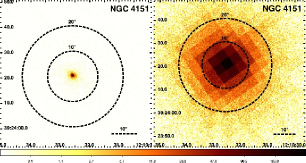
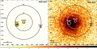
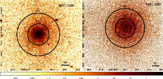
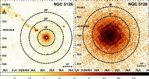
Figure 1: Images of NGC 4151, NGC 221, NGC 1399, and NGC 5128. The left hand panels are Chandra images and the right hand panels XMM-Newton images. Circles with different lines and colors indicate the extended regions for count estimations and nearby sources for the NGC 221 case. NGC 4151 is an example of a clear nuclear source, NGC 221 of a LLAGN surrounded by nearby objects, NGC 1399 of an AGN with substantial extended emission, and NGC 5128 of a LLAGN with jet-like emission presences.

We illustrate this procedure in Figure 1 using NGC 4151 as an example of a clearly isolated nuclear source, NGC 221 (also known as M32) as an example of a LLAGN surrounded by bright nearby objects, NGC 1399 as an example of diffuse emission, and NGC 5128 showing a LLAGN with a jet-like structure. Chandra and XMM-Newton images are in the left and right hand panels, respectively.

NGC 4151 is a well-known nearby ($D\sim 13.3$ Mpc, Mundell et al., 1999) Seyfert 1.5 galaxy (Osterbrock & Koski, 1976). Both images show that it is an isolated source. The Chandra net count difference of $\sim 20\%$ between the extraction region with radius of $1.5"$ ($1.3\times 10^{5}$) and that with radius of $20"$ ($\sim 1.7\times 10^{5}$) confirms that in NGC 4151 the contribution from the extended emission is negligible. Out of 53 LLAGNs, 22 sources appear to have an isolated central source.

The Chandra image of NGC 221 (top right panels of Figure 1) shows the presence of two additional sources inside of the $20"$ radius. They are indicated by solid lined circles. A source brighter than the AGN in NGC 221, ‘source1’ in Figure 1, is located $8.3"$ southeast of NGC 221 and a dimmer source (‘source2’) $20"$ away in the western direction. Although source1 and the nucleus of NGC 221 are clearly distinguishable with the sub-arcsecond spatial resolution of Chandra, the XMM-Newton image on the right hand panel reveals a single emission component. In this case, the XMM-Newton spectrum is dominated by the brightest off-nuclear source. As a consequence, the XMM-Newton observation of NGC 221 cannot be used to characterize the properties of the LLAGN. Using Chandra data, we find that $92\%$ of total counts ($1.4\times 10^{4}$) in $10"$ are from source 1 whereas the counts of NGC 221 are $6.1\times 10^{2}$. There were a total of 23 objects containing off-nuclear sources within $10"-20"$ radii from the central source. For six objects (NGC 2787, NGC 4278, NGC 4374, NGC 4945, NGC 4649, and NGC 5576) the central source emission dominates and the contribution from off-nuclear sources appears to be negligible. Therefore, in these cases, the XMM-Newton data can be used for the spectral analysis. For the remaining 5 sources (NGC 221, NGC 224, NGC 1023, NGC 3585, NGC 4291) only Chandra data can be used to investigate the AGN spectral X-ray properties given the significant contamination in the XMM-Newton data.

The left and right bottom panels of Figure 1 show the cases of two sources (NGC 1399 and NGC 5128) whose X-ray emission in the XMM-Newton extraction region is severely contaminated by extended emission and jet emission, respectively. Despite the fact that 12 sources are also classified as radio galaxies, only 3 (NGC 4486, NGC 4594, NGC 5128) show the presence of an extended jet-like structure in the Chandra images.

In summary, after the visual inspection of all Chandra images of our sample, 22 appear to be isolated sources (indicated by “iso” in the X-ray morphology classification reported in Table 2), 23 LLAGNs contain off-nuclear sources within 20” (“off” in Table 2), and the remaining have either significant extended emission (“ext” in Table 2) or jet-like structures (“jet”).

4 X-ray spectral analysis

We extracted spectra in the energy range from $0.3-10$ keV for all isolated sources and for those without significant off-nuclear contribution with XMM-Newton data (24 sources), and for the remaining 29 sources we used Chandra data. We grouped 20 or 15 counts per bin, which is appropriate for the use of the $\chi^{2}$ statistics. To increase the statistics for the XMM-Newton observation, we fitted simultaneously the EPIC pn, MOS1, and MOS2 spectra. For Chandra spectra if the number of counts per extraction region was low (e.g., $\leq 100$), the spectra were kept ungrouped and the C-stat statistic was used (Cash, 1979). Overall, we used the C-statistics for 24 Chandra spectra and 2 XMM-Newton spectra. All sources in our sample were systemically fitted with a base-line model comprising a power law (PL) and two absorption models, one fixed at the Galactic value and the other left free to vary to mimic the intrinsic local absorption. When necessary, Gaussian components were added to fit line-like features.

The spectral results are reported in Table 2. For sources with unconstrained intrinsic absorption value, we reported the upper limits. The vast majority of the sample have X-ray photon indices in the range from 1 to 3, with a few objects yielding very hard values ($\Gamma<1$). Unabsorbed luminosities $L_{\mathrm{X}}$ are in the range of $10^{38}-10^{43}$ erg s^-1, with the exceptions of NGC 221, NGC 224, and NGC 4486A that have low luminosities of order of $10^{36}-10^{37}$ erg s^-1. Overall, the spectral fits of 53 sources were in the range of $0.8\leq\chi^{2}_{red}\leq 1.5$ for the $\chi^{2}$ statistics and the C-statistic/dof also was in a similar range.

Table 2: Spectral Analysis

Source Name	Instrument	OSB ID	$N_{\rm H}$	$\Gamma$	$\log(L_{\rm x})$	Statistics	X-ray Mor.	$\log(L_{\rm X}/L_{\rm Edd})$	$R_{\rm X}$
(1)	(2)	(3)	(4)	(5)	(6)	(7)	(8)	(9)	(10)
IC 1459	X	0135980201	$0.16\pm 0.01$	$1.99\pm 0.02$	40.76	576.06/574	iso	-6.79	-1.00
IC 4296	X	0672870101	$0.09\pm 0.01$	$1.49\pm 0.02$	41.47	733.20/630	iso	-5.77	-2.88
NGC 221	C	5690	$\leq 0.02$	$2.29\pm 0.16$	35.92	32.90/24	off	-8.68	-2.62
NGC 224	C	1575	$0.03\pm 0.01$	$2.50\pm 0.09$	36.77	63.86/56	off	-9.51	-4.63
NGC 821	C	6314	$\leq 0.16$	$1.76\pm 0.48$	38.67	38.70/35 c	off	-7.07
NGC 1023	C	8464	$0.08\pm 0.03$	$2.14\pm 0.12$	38.66	135.36/179 c	off	-7.11
NGC 1068	C	344	$\leq 0.001$	$2.56\pm 0.02$	40.77	305.01/210	ext	-4.27	-1.59
NGC 1300	C	11775	$3.83\leq 0.77$	$2.24\pm 0.14$	39.68	85.37/107 c	iso	-6.28
NGC 1399	X	0400620101	$0.17\pm 0.01$	$3.02\pm 0.05$	39.87	1000.58/753	iso	-6.95
NGC 2748	C	11776	$0.15\pm 0.14$	$2.34\pm 0.65$	38.30	11.75/17 c	off	-7.48
NGC 2778	C	11777	$\leq 0.20$	$2.29\pm 0.57$	38.43	30.36/28 c	off	-6.89
NGC 2787	X	0200250101	$0.06\pm 0.02$	$2.03\pm 0.06$	39.09	131.82/115	off	-6.66	-1.87
NGC 3031	X	0657801801	$0.05\pm 0.01$	$2.06\pm 0.01$	40.27	999.93/896	iso	-5.74	-3.45
NGC 3115	C	11268	$0.03\pm 0.03$	$2.11\pm 0.20$	38.35	97.60/125 c	off	-8.74
NGC 3227	X	0400270101	$\cdots$	$1.41\pm 0.003$	42.06	2050.46/1890	iso	-3.23	-4.34
NGC 3245	C	2926	$\leq 0.23$	$1.83\pm 0.36$	39.27	39.93/57 c	iso	-7.19	-2.29
NGC 3377	C	2934	$0.15\pm 0.05$	$2.06\pm 0.23$	38.29	66.62/93 c	off	-7.88
NGC 3379	C	7076	$0.10\pm 0.04$	$2.26\pm 0.21$	38.33	89.83/113 c	off	-7.87
NGC 3384	C	11782	$\leq 0.21$	$1.83\pm 0.27$	38.55	51.15/73 c	off	-6.81
NGC 3585	C	9506	$0.08\pm 0.03$	$2.39\pm 0.20$	38.78	103.00/115 c	off	-7.86
NGC 3607	X	0099030101	$0.06\pm 0.04$	$2.63\pm 0.22$	38.85	33.15/35	iso	-7.34
NGC 3608	C	2073	$\leq 0.23$	$2.44\pm 0.31$	38.58	42.98/63 c	ext	-7.85
NGC 3998	X	0090020101	$0.01\pm 0.01$	$1.85\pm 0.01$	41.43	1159.15/1163	iso	-5.05	-3.40
NGC 4026	C	6782	$\leq 0.33$	$2.11\pm 0.55$	38.06	21.05/29 c	ext	-8.38
NGC 4151	X	0143500301	$\leq 0.08$	$-0.46\pm 0.00$	42.79	1899.16/1594	iso	-2.97	-4.59
NGC 4258	X	0400560301	$0.38\pm 0.01$	$2.10\pm 0.34$	40.45	1253.17/1142	iso	-5.24	-4.42
NGC 4261	X	0056340101	$\leq 0.02$	$0.82\pm 0.03$	40.94	561.75/441	iso	-5.91	-1.73
NGC 4278	X	0205010101	$0.02\pm 0.01$	$2.06\pm 0.01$	40.26	934.64/929	off	-7.05	-2.35
NGC 4291	C	11778	$\leq 0.10$	$2.11\pm 0.23$	39.12	75.50/87 c	off	-7.50
NGC 4303	X	0205360101	$\leq 0.18$	$2.90\pm 0.37$	39.06	49.45/43	iso	-5.70	-0.60
NGC 4342	C	12955	$\leq 0.08$	$1.90\pm 0.15$	38.62	159.76/182 c	off	-8.05
NGC 4374	X	0673310101	$\leq 0.02$	$2.16\pm 0.05$	39.68	347.37/315	off	-7.61	-0.91
NGC 4395	X	0142830101	$0.24\pm 0.01$	$0.96\pm 0.01$	40.16	3030.09/2394	iso	-2.99	-4.60
NGC 4459	X	0550540101	$0.20\pm 0.02$	$1.99\pm 0.09$	39.37	147.63/162	iso	-6.61
NGC 4473	C	4688	$\leq 0.28$	$1.70\pm 0.52$	38.97	22.96/28 c	ext	-7.25
NGC 4486	C	2707	$\leq 0.001$	$1.67\pm 0.01$	41.24	582.59/400	jet	-6.43	-1.41
NGC 4486A	C	11783	$\leq 0.21$	$1.47\pm 0.29$	37.00	57.15/61 c	ext	-8.24
NGC 4564	C	4008	$\leq 0.15$	$1.75\pm 0.29$	38.89	64.17/61 c	off	-7.06
NGC 4594	X	0084030101	$0.14\pm 0.01$	$1.85\pm 0.02$	40.51	551.35/574	jet	-6.36	-2.62
NGC 4596	C	11785	$\leq 0.16$	$1.48\pm 0.24$	39.28	58.83/69 c	off	-6.75
NGC 4649	X	0502160101	$0.06\pm 0.02$	$2.55\pm 0.02$	40.06	1254.12/811	off	-7.38	-2.61
NGC 4697	C	4730	$\leq 0.16$	$1.41\pm 0.19$	39.00	68.99/94 c	off	-7.40
NGC 4742	C	11779	$0.04\pm 0.04$	$1.76\pm 0.17$	39.15	95.84/135 c	off	-6.14
NGC 4945	X	0204870101	$\leq 0.03$	$0.03\pm 0.03$	40.13	633.61/502	off	-4.13	-1.96
NGC 5077	C	11780	$0.14\pm 0.06$	$1.88\pm 0.23$	39.73	78.05/83 c	iso	-7.28
NGC 5128	C	3965	$5.50\pm 0.13$	$-0.27\pm 0.02$	40.89	183.32/216	jet	-5.70	-1.04
NGC 5252	X	0152940101	$2.08\pm 0.01$	$1.11\pm 0.01$	43.11	2226.37/2050	iso	-4.00	-4.06
NGC 5576	X	0502480701	$\cdots$	$1.83\pm 0.19$	39.21	295.30/325 c	off	-7.16
NGC 5845	X	0021540501	$\leq 0.07$	$2.27\pm 0.34$	38.85	163.04/209 c	iso	-7.72
NGC 6251	X	0056340201	$0.04\pm 0.01$	$1.93\pm 0.02$	42.67	1211.77/1069	iso	-4.22	-1.66
NGC 7052	C	2931	$0.06\pm 0.04$	$2.71\pm 0.27$	40.24	68.57/79 c	iso	-6.47	-0.81
NGC 7457	C	11786	$\leq 0.19$	$1.41\pm 0.33$	38.36	25.89/39 c	iso	-6.36
NGC 7582	X	0204610101	$0.12\pm 0.01$	$0.07\pm 0.03$	41.13	1581.04/1044	iso	-4.72	-2.58

• • Columns 1 = source name, 2= observation ID, 3 = counts in source region, 4= intrinsic absorption value in units of $10^{22}$ cm^-2, 5 = photon index, 6 = unabsorbed luminosity in $2-10$ keV, 7 = $\chi^{2}$/degree of freedom: ^c C-statistic/degree of freedom, 8 = X-ray morphology (iso $-$ central AGN; off $-$ presence of nearby objects within 10 arc sec; ext $-$ diffused emission, jet $-$ jet-like structure emission), 9 = $\log(L_{\rm X}/L_{\rm Edd})$ 10 = X-ray radio-loudness parameter, $R_{\rm X}$($=\log(L_{\rm R}/L_{\rm X})$)

For completeness, for sources with both Chandra and XMM-Newton observations, we have compared the photon index and X-ray flux measured by the two satellites at different epochs. The vast majority of the AGNs shows consistent values with variations within the $3\sigma$ level. The only discrepancies are observed in objects that have poorly constrained Chandra spectra with $\Gamma$ either very steep ($>3$) or very flat ($<1$ or inverted spectra). We can therefore conclude that flux and spectral variability does not significantly affect our analysis.

Combining the X-ray luminosities inferred from the spectral analysis with the black hole masses from dynamical measurements, we derive the X-ray Eddington ratio, $L_{X}/L_{\mathrm{Edd}}$ ($L_{\rm 2-10\,keV}/L_{\rm Edd}$), for all the sources. Throughout the paper we use $L_{\mathrm{X}}$ to indicate the luminosity in the $2-10$ keV energy range, which is the most common band used in X-ray studies and allow a direct comparison with literature results. These values of $\log(L_{\rm X}/L_{\rm Edd})$, reported in Table 2, range between $-10$ and $-3$, with a mean of $-6.5\pm 1.5$. The distribution of $\log(L_{\rm X}/L_{\rm Edd})$ for each optical class is plotted in Figure 2. Assuming a bolometric correction of $15-30$, which is appropriate for low-accreting AGNs (see, e.g., Vasudevan & Fabian 2009), we obtain Eddington ratio values $\log(L_{\rm bol}/L_{\rm Edd})$ ranging between $-8.8$ and $-1.8$ with a mean of $-5.3$, which confirms that this sample comprises only low-accreting AGNs.

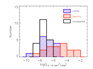
Figure 2: Distribution of $L_{X}/L_{\mathrm{Edd}}$. The histogram filled with positive slopes indicate LINERs, the negative slopes filled represent Seyferts, and the empty one unclassified AGNs.

Very flat X-ray spectra are often associated with heavily absorbed AGNs. In the most extreme cases (i.e., for Compton-thick sources with $N_{\rm H}>10^{24}\,{\rm cm}^{-2}$), the direct coronal emission is completely absorbed and the detected X-rays are thought to be produced by reflection. Since in these sources the estimated $L_{\mathrm{X}}$ is severely underestimated and $\Gamma$ is not representative of the direct emission, it is not possible to extend the X-ray scaling method to Compton-thick AGNs. For this reason, it is crucial to identify (and exclude from further analysis) Compton-thick sources. Typically, two different approaches are used to find Compton-thick candidates: 1) the detection of Fe K$\alpha$ lines with large equivalent width (EW$>1$keV) and 2) the use of the $T_{\rm ratio}=F_{\rm 2-10keV}/F_{\rm[OIII]}$ parameter (where $F_{\rm[OIII]}$ is corrected for optical reddening), with the assumption that the X-ray flux is associated with the absorbed AGN component, whereas the O[III] flux is considered a reliable indicator of the isotropic emission since it is mostly produced in the unobscured narrow line region (Bassani et al. 1999). Past studies have shown that Compton-thick objects are characterized by values of T below 1.

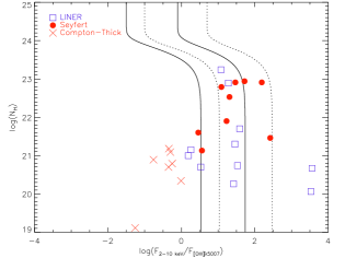
Figure 3: Plot of $\log(N_{\rm H})$ vs. $\log(F_{\rm 2-10\,keV}/F_{\rm[OIII]})$. The filled circles indicate Seyfert galaxies and the open squares LINERs. The cross mark “x” was used to indicate the Compton-thick candidates. The solid lines indicate the expected correlation derived by Cappi et al. (2006) assuming that $L_{\mathrm{X}}$ is absorbed by the measured $N_{\rm H}$ and a $1\%$ reflected component. Similarly the dashed lines indicate the correlation derived by Maiolino et al. (1998).

We have computed the T factor for all the objects of our sample with optical line measurements. The results are plotted in Figure 3 where the lines represent the expected correlation between T and $N_{\rm H}$ for Seyfert galaxies under the assumption that the X-ray flux is absorbed by the measured $N_{\rm H}$. Figure 3, combined with results from the spectral analysis showing flat spectra and in some cases a Fe K$\alpha$ line with large EW, suggests that 8 sources (NGC 1068, NGC 2748, NGC 3607, NGC 3245, NGC 4303, NGC 4374, NGC 4945, NGC 7582) may be genuine Compton-thick candidates, in agreement with independent findings in the literature (Bianchi et al. 2009; Cappi et al. 2006; Gon$\acute{\rm z}$alez-Martin et al. 2009; Marinucci et al. 2012; Yaqoob 2012). To be conservative, we exclude from further analysis these 8 objects.

Sources with flat spectra but without evidence for Compton thickness and sources that showed substantial residuals when fitted with our simple base-line model were re-fitted with more complex models. These spectral models may comprise a thermal component (apec in Xspec) to account for galaxy contribution, a blackbody to mimic a soft excess, a partial covering model (zpcfabs) to account for absorbers with patchy geometry and a reflection component (pexrav). This additional spectral analysis yielded steeper photon indices as indicated by Table 3 that reports the most relevant spectral parameters.

In summary, all sources were reasonably well fitted by either an absorbed power law or slightly more complex models, yielding $\Gamma$ values in the range $1.3-3$ and $L_{\mathrm{X}}$ between $10^{37}$ and $10^{43}$ erg s^-1.

Table 3: Spectral Analysis $-$ For Objects with Very Flat Spectra

Source Name	Model	$N_{\rm H}$	R	Ebreak	$\Gamma$	FeK$\alpha$	EW	$\log(L_{\rm x})$	$\chi^{2}$/dof
(1)	(2)	(3)	(4)	(5)	(6)	(7)	(8)	(9)	(10)
NGC 5128	wabs(bknpo+pexrav)	$8.09\pm 0.27$	$0.63\pm 0.09$	$4.68\pm 0.07$	$0.22\pm 0.01$	$6.42\pm 0.03$	$0.03$	40.88	191.36/200
Source Name	Model	$N_{\rm H}$	CF	kT	$\Gamma$	Fe K$\alpha$	EW	$\log(L_{\rm x})$	$\chi^{2}$/dof
			(11)	(12)
NGC 1300	pcfabs(pow)	$3.83\pm 0.77$	$0.96\pm 0.02$		$2.24\pm 0.14$			39.68	85.37/107c
NGC 3031	wabs(bb+pow)	$0.00$		$0.29\pm 0.02$	$1.90\pm 0.01$			39.38	985.49/895
NGC 3115	pcfabs(pow)	$0.13\pm 0.08$	$0.70\pm 0.33$		$2.34\pm 0.24$			38.09	80.94/126
NGC 3227	pcfabs(pow)+gauss	$6.16\pm 0.15$	$0.91$		$1.39\pm 0.01$	$6.38\pm 0.01$	$0.06\pm 0.02$	41.77	1866.78/1739
NGC 4151	pcfabs(pow+apec+gauss)	$3.38\pm 0.02$	$0.95$	$0.14$	$1.33\pm 0.01$	$6.37\pm 0.01$	$0.06\pm 0.02$	42.88	2617.68/1892
NGC 4258	pow+wabs(pow)	$8.74\pm 0.20$			$1.70\pm 0.02$			40.51	966.56/945
NGC 4261	pow+pcfabs(pow)	$7.71\pm 0.62$			$1.65\pm 0.03$			41.16	457.95/442
NGC 4342	pcfabs(pow)		$0.78\pm 0.02$		$1.61\pm 0.12$			39.81	172.65/173c
NGC 4395	pcfabs(apec+pow)	$0.79\pm 0.02$	$0.72$	$0.19$	$1.11\pm 0.01$			39.96	3197.11/2394
NGC 4596	pcfabs(pow)	$17.20$	$0.05$		$1.89\pm 0.36$			38.86	36.87/67
NGC 4649	pcfabs*apec*pow	$0.13\pm 0.01$	$0.82\pm 0.02$	$0.87$	$1.64\pm 0.03$			40.12	1250.62/798
NGC 4697	pcfabs(pow)	$0.19\pm 0.07$	$\leq 0.79$		$2.08\pm 0.30$			38.25	50.27/91
NGC 5128	abs(apec+pow)	$8.14\pm 0.16$		$0.11$	$0.32\pm 0.01$			40.40	245.92/216
NGC 6251	pcfabs*apec*pow	$0.40\pm 0.03$	$0.54\pm 0.02$	$0.61\pm 0.03$	$1.83\pm 0.01$			42.72	1143.05/1059
NGC 7052	pcfabs(bb+pow)			$0.16\pm 0.03$	$1.76\pm 0.36$			40.43	13.46/15
NGC 7457	wabs(apec+pow)	$0.29\pm 0.09$		$0.13\pm 0.02$	$1.52\pm 0.39$			38.50	11.17/12

• Columns 1 = source name, 2 = model used, 3 = intrinsic absorption value in units of $10^{22}$ cm^-2, 4 = Reflection Factor ($0\leq{\rm R}\leq 1$: 0 $-$ no reflection component and 1 $-$ isotropic source above disk), 5 = energy break (keV), 6 = photon index, 7 = Fe K$\alpha$ line (keV), 8 = equivalent width (keV), 9 = unabsorbed luminosity in $2-10$ keV, 10 = $\chi^{2}$/degree of freedom (^c indicates C-statistic/degree of freedom), 11 = demensionless coverage fraction, 12 = temperature of soft excess in units of keV.
  

4.1 X-ray Radio-loudness

Combining the X-ray luminosity inferred from the spectral analysis and the radio luminosity from the literature, we computed the X-ray radio loudness parameter, $R_{\rm X}=L(6\rm{cm})/L_{2-10\,{\rm keV}}$, which was introduced by Terashima & Wilson (2003) to reduce the extinction that affects the optical emission used in the classical radio-loudness parameter. The values of $R_{\rm X}$ for each objects are reported in Table 2. For the 26 sources (9 LINERs, 14 Seyferts, 3 unclassified) for which the radio data are available, $\log(R_{\rm X})$ ranges between $-5$ and $0$ with a mean of $-2.5\pm 1.3$. These values are consistent with those of the sample of low-luminosity Seyfert galaxies analyzed by Panessa et al. (2007). Similar to Panessa et al. (2007) we did not find any correlation between $R_{\rm X}$ and $L_{\mathrm{X}}$, whereas there is suggestive evidence for an anti-correlation between $R_{\rm X}$ and $L_{X}/L_{\mathrm{Edd}}$. However, unlike Panessa et al. (2007) the anti-correlation in our sample is not statistically significant: the negative slope is consistent with 0 within $2\sigma$s. This can be explained either but the limited number of objects with radio data in our sample or by the fact that our objects are accreting at a much lower level and in this regime no correlation is expected between radio-loudness and Eddington ratio, as demonstrated by Sikora et al. (2007).

We also looked for any correlation between $\Gamma$ and $R_{\rm X}$ and plotted of $\Gamma$ versus $R_{\rm X}$ is in Figure 4. When all objects with $R_{\rm X}$ are included, there is no evidence for any correlation (the Spearman’s $\rho-$rank is $0.45$ with a probability of $P=0.03$). If we exclude the Compton-thick candidates and the source with very low $\Gamma$, then a weak positive correlation of $\Gamma=(0.17\pm 0.05)R_{\rm X}+(2.16\pm 0.22)$ with the RMS value of $0.22$ is found.

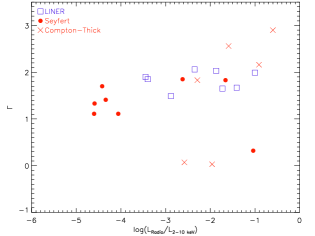
Figure 4: Plot of $\Gamma$ vs. $\log(L(6\rm{cm})/L_{2-10\,{\rm keV}})$. Open squares were used to indicate LINERs, filled circles for Seyferts, and crosses for Compton-thick candidates.

5 Estimation of $M_{\rm BH}$ with X-rays

5.1 X-ray Scaling Method

In a recent study on GBHs, Shaposhnikov & Titarchuk (2009) showed that spectral transitions of different GBHs present two similar positive correlations between temporal and spectral properties: 1) a correlation between the quasi periodic oscillation (QPO) frequency and the photon index and 2) a correlation between $N_{BMC}$, the normalization of the bulk Comptonization (BMC) model, and the photon index. Because different BHs show similar trends in the $\Gamma-\mathrm{QPO}$ and $\Gamma-N_{BNC}$ diagrams, it can be shown that $M_{BH}$ (and distance) of any GBH can be determined by simply shifting this self-similar function until it matches the spectral pattern of a GBH of known $M_{BH}$ and distance (considered as a reference source).

In the following, we briefly describe the Comptonization model used in the X-ray scaling method, the basic characteristics of the technique utilized to estimate $M_{\rm BH}$, and the main results obtained applying this method to AGNs.

It is widely accepted that the X-ray emission associated with BH systems is produced by the Comptonization process in the corona. The BMC model is a simple and robust Comptonization model which equally well describes thermal and bulk Comptonization (Titarchuk et al., 1997). The BMC model is characterized by four parameters: (1) the temperature of the thermal seed photons, $kT$, (2) the energy spectral index $\alpha$ (related to the photon index by the relation $\Gamma$$=\alpha+1$), (3) $\log(A)$ which is related to the Comptonization fraction by $f=A/(1+A)$ (where $f$ is the ratio between the number of Compton scattered photons and the number of seed photons), and (4) the normalization, $N_{\mathrm{BMC}}$ which depends on the luminosity and the distance, ($N_{\mathrm{BMC}}$ $\propto L/d^{2}$).

The X-ray scaling method, based on two diagrams $\Gamma$$-\nu_{QPO}$ and $\Gamma$$-$$N_{\mathrm{BMC}}$, allowed the estimate of $M_{\rm BH}$ and distance in several GBHs by scaling the temporal and spectral properties of a reference GBH. However, the much longer timescales of AGNs and the absence of detectable QPOs do not allow the use of the $\Gamma$ $-$ QPO diagram. On the other hand, the $\Gamma$ $-$ $N_{\mathrm{BMC}}$ plot can be easily extended to AGNs assuming that AGNs follow a similar spectral evolution as GBHs. This method relies on the direct dependence of the BMC normalization on $M_{\rm BH}$: $N_{BMC}=L/d^{2}$, where $L\propto\eta\dot{m}M_{BH}$ is the accreting luminosity, $\eta$ is the radiative efficiency and $\dot{m}$ the accretion rate in Eddington units. Therefore, the normalization, $N_{\mathrm{BMC}}$, can be expressed as a function of $M_{BH}$: $N_{BMC}\propto\eta\dot{m}M_{BH}/d^{2}=M_{\rm BH}/d^{2}$, which is derived assuming that different BHs in the same spectral state (defined by the value of $\Gamma$) are characterized by similar values of $\eta$ and $\dot{m}$.

With this X-ray scaling method, Gliozzi et al. (2011) estimated $M_{BH}$ for a well defined sample of AGNs accreting at moderate/high level ($\dot{m}\gg 1\%$) whose BH mass was determined via reverberation mapping and which had good quality XMM-Newton archival data. The good agreement between the $M_{BH}$ values determined by these two methods (the RMS around the one-to-one correlation between $\log M_{\rm BH,scaling}$ and $\log M_{\rm BH,RM}$ is 0.35 using GRO J1655-40 as a reference) confirmed the validity of this novel technique that can be successfully used for both sMBHs and SMBHs.

At very low accreting rate however, X-rays are likely to be produced by different mechanisms (for example by advection dominated accretion flows, ADAFs, or can be directly related to jet emission). Moreover, the applicability of the X-ray scaling method is questionable, since it is based on the similarity of the spectral transition of BHs at relatively high accretion rate ($L_{X}/L_{\mathrm{Edd}}$$\geq 10^{-2}$), which is described by a positive correlation in the $\Gamma$$-$flux diagram.

To test whether the scaling method can be applied to LLAGNs, we fitted their spectra with the BMC model. LLAGNs with $\Gamma$$=1.3-3$ were compared to different spectral evolution trends of GBHs. The X-ray scaling method results are shown in Figure 5. There is a clear inconsistency between the values from the scaling method and those obtained from dynamical methods.

The vast majority of the $M_{\rm BH}$ inferred from the scaling methods lie well below the one-to-one correlation (indicated by the solid line), and appear to be underestimated by $2-4$ orders of magnitude. This indicates that the X-ray scaling method cannot be used to constrain the $M_{\rm BH}$ of very low-accreting AGNs. The only noticeable exceptions are NGC 3227 and NGC 4151, which appears to be fully consistent with their corresponding dynamical estimate, and NGC 4395 and NGC 5252, that are marginally consistent. Importantly, these sources have the highest $L_{X}/L_{\mathrm{Edd}}$ values in our sample and suggest that the scaling method is still valid for $L_{X}/L_{\mathrm{Edd}}$ of the order of $10^{-3}-10^{-4}$.

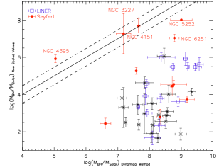
Figure 5: $M_{\rm BH}$ values obtained with the scaling method plotted vs. $M_{\rm BH}$ values measured by dynamical method. The Seyfert sample is plotted with filled circles, open squares for LINERs, and crosses for unclassified LLAGNs. The solid line is to indicate the one-to-one correlation. Five objects with $L_{X}/L_{\mathrm{Edd}}$ ${}^{<}_{\sim}10^{-4}$ are labeled next to the data points.

5.2 $\Gamma-L_{\rm X}/L_{\mathrm{Edd}}$ Anti-Correlation

We tested whether our LLAGN sample showed any evidence for an anti-correlation in the $\Gamma$ vs. $L_{X}/L_{\mathrm{Edd}}$ plot. The results, obtained using the photon index and the luminosity in the $2-10$ keV range, are shown in Figure 6 and support the existence of an anti-correlation, whose best-fit is indicated by the solid line and the $1\sigma$ uncertainty with dashed lines.

The slope and y-intercept of best-fit results of LINERs, Seyferts, unclassified AGNs, and the combination of LINERs and Seyferts and all are reported in Table 4. There is suggestive evidence for an anti-correlation for LINERs, Seyferts, and the combination of all, when the results from the fitting of a simple PL model are used (Case 1 Table 4) and of more complex spectral models (Case 2 Table 4). When all AGN classes are combined, the significant negative correlations are confirmed by a non-parametric correlation analysis based on Spearman’s $\rho-$rank coefficient which yields a value of $-0.42$ ($P=8.19\times 10^{-3}$) for Case 1, and $-0.65$ ($P=1.44\times 10^{-6}$) for Case 2. We also tested the anti-correlation test for Case 2 without NGC 1399 ($\Gamma$$\approx 3$) and NGC 5128 ($<1$) and the best-fit parameters remained consistent within the $1\sigma$ uncertainty. For completeness, in Table 4 we also report the results of the correlation analysis between $\Gamma$ and $L_{\mathrm{X}}$ (e.g., Emmanoulopoulos et al. (2012)) and show the $\Gamma-L_{\rm X}$ plot in Figure 7.

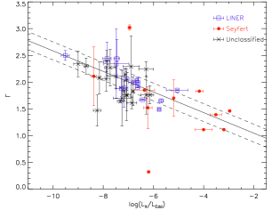
Figure 6: Anti-correlation of $\Gamma-L_{\rm X}/L_{\rm Edd}$. The LINER data are indicated by open squares whereas the filed circles represent Seyferts and crosses unclassified ones. The best-fit (with parameters in Table for Case 2 ALL in Table 4) is indicated with the solid line with the dashed lines showing the $1\sigma$ uncertainty.

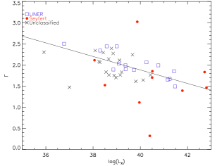
Figure 7: Anti-correlation of $\Gamma-L_{\rm X}$. The LINER data are indicated by open squares whereas filled circles represent Seyferts and crosses for unclassified ones. The best-fit (with parameters for Case 2 ALL in Table 4) is indicated with the solid line.

Table 4: X-ray Properties Correlation Analysis Results

AGN Class	Slope	Y-int.	RMS
(1)	(2)	(3)	(4)
$\Gamma$$-$$L_{X}/L_{\mathrm{Edd}}$ Analysis Results
Case 1 $-$ use of results from the base-line model
LINER	$-0.25\pm 0.09$	$0.19\pm 0.62$	0.33
Seyfert	$-0.30\pm 0.16$	$-0.17\pm 0.88$	0.84
L+S†	$-0.29\pm 0.08$	$-0.11\pm 0.49$	0.61
Unclassified	$-0.20\pm 0.15$	$0.49\pm 1.11$	0.45
ALL	$-0.26\pm 0.06$	$0.03\pm 0.39$	0.55
Case 2 $-$ use of results from the complex model
LINER	$-0.22\pm 0.05$	$0.46\pm 0.32$	0.16
Seyfert	$-0.17\pm 0.11$	$0.68\pm 0.63$	0.58
L+S†	$-0.20\pm 0.05$	$0.56\pm 0.34$	0.41
Unclassified	$-0.13\pm 0.08$	$0.97\pm 0.60$	0.26
ALL	$-0.18\pm 0.04$	$0.66\pm 0.25$	0.35
$\Gamma$$-$$L_{\mathrm{X}}$ Analysis Results
Case 1
LINER	$-0.21\pm 0.07$	$10.41\pm 2.77$	0.32
Seyfert	$-0.24\pm 0.18$	$11.24\pm 7.50$	0.90
L+S†	$-0.26\pm 0.09$	$12.11\pm 3.58$	0.66
Unknown	$-0.01\pm 0.12$	$2.34\pm 4.74$	0.47
Comb	$-0.20\pm 0.06$	$9.63\pm 2.40$	0.60
Case 2
LINER	$-0.19\pm 0.04$	$9.43\pm 1.39$	0.17
Seyfert	$-0.10\pm 0.13$	$5.71\pm 5.26$	0.62
L+S†	$-0.17\pm 0.06$	$8.72\pm 2.39$	0.45
Unknown	$-0.08\pm 0.06$	$5.08\pm 2.47$	0.27
Comb	$-0.16\pm 0.04$	$8.28\pm 1.45$	0.27

Note: Column List $-$ (1) AGN class; (2) a best-fit slope; (3) a best-fit intercept’ (4) RMS for the best-fit. All Compton-thick sources are excluded during the anti-correlation between $\Gamma$ and $L_{X}/L_{\mathrm{Edd}}$ confirmation.
^† $-$ LINERs and Seyfert galaxies only

The existence of a robust anti-correlation between $\Gamma$ and $L_{X}/L_{\mathrm{Edd}}$ offers an alternative X-ray-based method to estimate $M_{\rm BH}$ in low-accreting BHs. Since $L_{\rm Edd}$ is a linear function of $M_{\rm BH}$, one can solve the equation for $M_{\rm BH}$, and hence constrain it by plugging the values of $\Gamma$ and $L_{\mathrm{X}}$ as well as the intercept and the slope of the anti-correlation:

$$\log(M_{BH})=\log(L_{\mathrm{X}})-38.11-\left[\frac{\Gamma-B}{A}\right]$$ (1)

where A is the best-fit slope, B is the best-fit y-intercept, and the constant 38.11 comes from the definition $L_{\mathrm{Edd}}=1.3\times 10^{38}(M_{BH}/M_{\odot})$ erg s^-1.

5.3 $M_{\rm BH}$ Computation

We estimated $M_{\rm BH}$ for the sources in Table 1 (except for 8 Compton-thick candidates) using the Equation 1 with the best-fitting parameters corresponding all AGN classes for both Case 1 (spectral results from the PL model) and Case 2 (spectral results from more complex models).

The $M_{\rm BH}$ values for the 47 LLAGNs from the anti-correlation of $\Gamma$$-$$L_{X}/L_{\mathrm{Edd}}$ ($M_{\rm BH,X}$) and the ratio between the $M_{\rm BH,X}$ and the corresponding values determined with dynamical methods ($M_{\rm BH,dyn}$) are reported in Table 5, with columns 2 and 3 referring to Case 1 and columns 4 and 5 to Case 2. The uncertainty of $M_{\rm BH,X}$ was derived from the parameter’s uncertainty in Equation (1).

Table 5: $M_{\rm BH}$ Estimation of LLAGN

LLAGN	$\log(M_{\rm BH,X})$	$\log(\frac{M_{\rm BH,X}}{M_{\rm BH,dyn}})$	$\log(M_{\rm BH,X})$	$\log(\frac{M_{\rm BH,X}}{M_{\rm BH,dyn}})$
(1)	(2)	(3)	(4)	(5)
LINER
I 1459	$9.78\pm 0.02$	$0.34\pm 0.20$	$9.56\pm 0.10$	$0.12\pm 0.22$
I 4296	$8.86\pm 0.38$	$-0.27\pm 0.38$
N 224	$7.98\pm 0.22$	$-0.19\pm 0.27$
N 2748	$8.52\pm 1.79$	$0.85\pm 1.85$
N 2787	$8.25\pm 0.07$	$0.61\pm 0.09$	$8.07\pm 0.25$	$0.43\pm 0.25$
N 3031	$9.54\pm 0.29$	$1.64\pm 0.30$	$7.89\pm 0.03$	$-0.01\pm 0.10$
N 3608	$9.14\pm 0.44$	$0.82\pm 0.47$
N 3998	$9.90\pm 0.16$	$1.53\pm 0.46$	$9.60\pm 0.19$	$1.23\pm 0.47$
N 4261	$5.99\pm 1.01$	$-2.75\pm 1.01$	$8.84\pm 0.58$	$0.10\pm 0.58$
N 4278	$9.53\pm 0.29$	$0.33\pm 0.29$	$9.38\pm 0.02$	$0.18\pm 0.02$
N 4459	$8.39\pm 0.30$	$0.52\pm 0.31$	$8.17\pm 0.43$	$0.30\pm 0.44$
N 4486	$9.31\pm 0.18$	$-0.25\pm 0.22$
N 4596	$6.64\pm 1.26$	$-1.28\pm 1.27$	$7.77\pm 1.38$	$-0.15\pm 1.39$
N 5077	$8.60\pm 0.87$	$-0.30\pm 0.90$
Seyfert
N 1399	$12.32\pm 3.68$	$3.61\pm 3.68$
N 3227	$9.11\pm 0.33$	$1.93\pm 0.40$	$7.70\pm 0.66$	$0.52\pm 0.70$
N 4026	$7.80\pm 1.94$	$-0.53\pm 1.95$	$8.28\pm 2.34$	$-0.05\pm 2.34$
N 4151	$3.72\pm 4.88$	$-3.93\pm 4.88$	$8.48\pm 0.73$	$0.83\pm 0.73$
N 4258	$9.85\pm 0.88$	$2.27\pm 0.88$	$8.02\pm 2.00$	$0.44\pm 2.00$
N 4395	$5.55\pm 0.79$	$0.51\pm 0.79$	$4.56\pm 1.13$	$-0.48\pm 1.13$
N 4594	$9.06\pm 0.04$	$0.30\pm 0.41$	$8.77\pm 0.09$	$0.01\pm 0.42$
N 5128	$2.45\pm 4.44$	$-6.03\pm 4.44$	$3.91\pm 2.96$	$-4.57\pm 2.96$
N 5252	$9.07\pm 0.66$	$0.07\pm 0.75$
N 6251	$11.49\pm 0.12$	$2.71\pm 0.19$	$10.88\pm 0.07$	$2.10\pm 0.16$
N 7457	$5.48\pm 1.67$	$-1.13\pm 1.68$	$6.01\pm 1.82$	$-0.60\pm 1.83$
Unclassified
N 221	$6.38\pm 0.19$	$-0.11\pm 0.21$	$6.41\pm 0.15$	$-0.08\pm 0.18$
N 821	$7.08\pm 1.97$	$-0.55\pm 1.97$
N 1023	$8.20\pm 0.04$	$0.54\pm 0.06$
N 1300	$3.69\pm 1.75$	$-4.16\pm 1.77$	$9.55\pm 0.01$	$1.70\pm 0.29$
N 2778	$8.48\pm 1.54$	$1.27\pm 1.57$
N 3115	$8.48\pm 0.93$	$-0.50\pm 0.95$	$8.78\pm 0.57$	$-0.20\pm 0.60$
N 3377	$8.17\pm 1.76$	$0.11\pm 1.77$
N 3384	$7.25\pm 4.40$	$0.00\pm 4.40$
N 3585	$9.17\pm 0.09$	$0.64\pm 0.15$
N 4291	$8.56\pm 0.47$	$0.05\pm 0.58$
N 4342	$7.68\pm 2.28$	$-0.88\pm 2.29$	$7.66\pm 0.63$	$-0.90\pm 0.66$
N 4473	$7.16\pm 2.18$	$-0.95\pm 2.21$
N 4564	$7.27\pm 1.22$	$-0.57\pm 1.22$
N 4649	$10.99\pm 0.73$	$1.66\pm 0.74$	$8.08\pm 0.29$	$-1.25\pm 0.31$
N 4697	$6.09\pm 1.12$	$-2.20\pm 1.12$	$8.35\pm 2.72$	$0.06\pm 2.72$
N 4742	$7.39\pm 0.60$	$0.21\pm 0.62$	$7.11\pm 1.14$	$-0.07\pm 1.15$
N 5576	$7.91\pm 3.42$	$-0.35\pm 3.42$
N 5845	$8.83\pm 0.72$	$0.37\pm 0.75$
N 7052	$11.72\pm 0.03$	$3.12\pm 0.22$	$8.67\pm 1.29$	$0.07\pm 1.31$
N 4486A	$4.32\pm 1.46$	$-2.81\pm 1.47$	$4.32\pm 1.46$

Note : (1) = LLAGN name; (2) & (3) = computed $M_{\rm BH}$ values with Case 1 best-fit parameters and the corresponding ratio between $M_{\rm BH,X}$ and $M_{\rm BH,dyn}$ values; (4) & (5) = computed $M_{\rm BH}$ values with Case 2 best-fit parameters and the corresponding ratio between $M_{\rm BH,X}$ and $M_{\rm BH,dyn}$ values

With few exceptions, we found a good agreement between the $M_{\rm BH}$ values determined with this anti-correlation and their corresponding dynamical values. These findings are illustrated in Figure 8 where we plot the $M_{\rm BH}$ values obtained with these two methods along the y- and x-axis, respectively. The apparent visual correlation is formally confirmed by the statistical analysis performed using the mpfitexy routine (Markwardt 2009; Williams, Bureau & Cappellari 2010). The best-fit parameters, the slope and intercept, with their $1\sigma$ uncertainty and the RMS from the one-to-one correlation for each LLAGN class and for the combination of all are reported in Table 6. The distribution of the ratio between computed $M_{\rm BH,X}$ and its corresponding $M_{\rm BH,dyn}$ for Case 2 is shown Figure 9.

We also investigated whether X-ray radio-loudness plays a role in the mass determination. To this end, we have divided our sample between radio-quiet and radio-loud objects using as the threshold $\log R_{\rm X}\geq-2.8$ (Panessa et al. 2007). The values of $\log(M_{\rm BH,X}/M_{\rm BH,dyn})$ for radio-quiet and radio-loud objects are respectively $0.29\pm 0.54$ and $0.55\pm 1.17$, which are consistent within the errors. This suggests that radio-loudness does not affect the mass determination with this X-ray method.

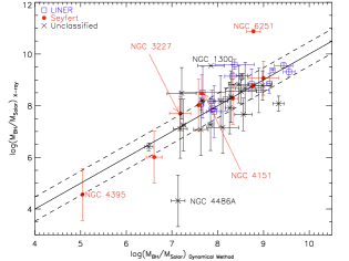
Figure 8: $M_{\rm BH}$ values obtained using the $\Gamma-L_{\rm X}/L_{\mathrm{Edd}}$ anti-correlation parameters vs. dynamically measured $M_{\rm BH}$ values. The open squares are used to indicate LINERs, filled circles for Seyferts, and X marks for unclassified sources. The one-to-one correlation is represented by the solid line whereas the dashed lines indicate the uncertainty.

Table 6: $M_{\mathrm{BH}}$ Correlation Analysis Results

Class	Slope	Y-int.	Spearman(Prob.)	RMS
(1)	(2)	(3)	(4)	(5)
Case 1
LINER	$0.56\pm 0.46$	$4.06\pm 3.96$	0.45($1.06\times 10^{-1}$)	1.09
Seyfert	$1.16\pm 0.36$	$-0.15\pm 2.82$	0.36($2.72\times 10^{-1}$)	2.75
Unclassified	$1.70\pm 0.41$	$-5.41\pm 3.32$	0.64($2.37\times 10^{-3}$)	1.54
ALL	$1.08\pm 0.22$	$-0.23\pm 1.80$	0.55($9.53\times 10^{-5}$)	1.81
Case 2
LINER	$0.77\pm 0.45$	$2.12\pm 3.89$	0.72($3.48\times 10^{-3}$)	0.50
Seyfert	$1.38\pm 0.37$	$-2.52\pm 2.94$	0.97($2.16\times 10^{-5}$)	0.83
Unclassified	$0.91\pm 0.38$	$0.68\pm 3.05$	0.61($4.37\times 10^{-3}$)	0.93
ALL	$1.00\pm 0.23$	$0.23\pm 1.89$	0.74($1.50\times 10^{-8}$)	0.79

Note : (1) AGN Class; (2) best-fit slope; (3) best-fit intercept; (4) Spearman’s $\rho-$rank and its following probability; (5) RMS from the one-to-one correlation

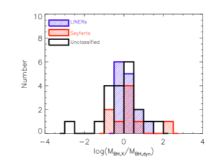
Figure 9: Histogram of $\log(M_{\rm BH,X}/M_{\rm BH,dyn})$ where $M_{\rm BH,X}$ refers to Case 2 (spectral results from more complex models). The histogram filled with positive slopes indicate LINERs, the negative slopes filled one is used for Seyferts, and the empty one for unclassified AGNs.

In summary, we computed $M_{\rm BH}$ for 47 LLAGNs based on the anti-correlation between $\Gamma$$-$$L_{X}/L_{\mathrm{Edd}}$. The vast majority of the $M_{\rm BH}$ values are in good agreement with their dynamical values within a factor of $5-6$ (RMS $\sim 0.8$).

6 Discussion

In this work, we performed a systematic and homogeneous re-analysis of the X-ray spectra for a sample of LLAGNs with $M_{\rm BH}$ dynamically constrained with the aim to test the validity and the limitations of two X-ray-based methods to determine $M_{\rm BH}$. The first method is based on the scale-invariance of X-ray spectral properties of BHs at all scales, whereas the second one is based on the anti-correlation of $\Gamma$ vs. $L_{X}/L_{\mathrm{Edd}}$ at very low accretion rates.

6.1 X-ray Scaling Method

In our recent work, we demonstrated that the X-ray scaling method, developed for and tested on GBHs (Shaposhnikov & Titarchuk 2009), can be successfully applied to AGNs with moderate/high accretion rate (Gliozzi et al. 2011). Specifically, using self-similar spectral patterns from different GBH reference sources we derived the $M_{\rm BH}$ values of a selected sample of bright AGNs and then compared them with the corresponding values obtained from the reverberation mapping technique. The tight correlation found in the $\log(M_{\rm BH,scal})$ and $\log(M_{\rm BH,RM})$ plane (RMS $=0.35$ for the most reliable reference source, GRO J1655-40, and RMS${}_{\rm avg}\,=0.53$ obtained by taking the average of five different reference patterns) demonstrates that the values of $M_{\rm BH}$ obtained with the scaling method are fully consistent with the reverberation mapping results within the respective uncertainties.

In this work, we have tested the limits of applicability of this scaling method to low accreting AGNs with typical $L_{X}/L_{\mathrm{Edd}}$ ratio of the order of $10^{-6}-10^{-7}$, which correspond to very low Eddington ratios ($<10^{-4}$) for any reasonable bolometric correction. In our starting sample, only three objects have $L_{X}/L_{\mathrm{Edd}}$ that are not extremely low: NGC 3227, NGC 4151, and NGC 4395 (all have $L_{X}/L_{\mathrm{Edd}}$ $\sim 10^{-3}$ and thus $L_{\rm bol}/L_{\rm Edd}\sim 10^{-2}$). The resulting $M_{\rm BH}$ values derived for the LLAGN sample from the X-ray scaling method are systematically lower than the dynamically inferred values by three or four orders of magnitude, indicating that the X-ray scaling method cannot be utilized for BHs in the very low accreting regime. The only notable exceptions are NGC 3227, NGC 4151, and NGC 4395 for which the derived $M_{\rm BH}$ are consistent with the dynamical values.

Paradoxically, the apparent failure of the scaling method, when applied to AGNs accreting at very low accretion rates, provides indirect support to this method. Indeed, it demonstrates that the agreement between $M_{\rm BH}$ values determined with the scaling method and the reverberation mapping values is not obtained by chance but is based on a common spectral evolution (the steeper when brighter spectral trend), which is systematically seen in highly-accreting AGNs and GBHs in their transition between the low-hard state and the soft-high state. This conclusion is further reinforced by the agreement between $M_{\rm BH,scal}$ and their dynamical values that was obtained for NGC 3227, NGC 4151, and NGC 4395, the only sources of this sample with accretion rate close to $10^{-2}$.

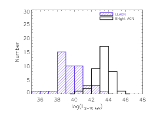
Figure 10: Histogram of $\log(L_{\rm X})$ and $\log(L_{\rm bol}/L_{\rm Edd})$ for our sample of LLAGNs and reverberation mapping AGNs in Gliozzi et al. (2011). The histogram filled with negative slopes indicates LLAGNs and the empty one for bright AGNs in both panels.

In Figure 10 we show the histogram of the X-ray luminosity (left panel) and of $L_{\rm bol}/L_{\rm Edd}$ (right panel) for the reverberation mapping sample used by Gliozzi et al. (2011) and the LLAGN sample utilized in the present work. The two distributions appear to be distinct as formally demonstrated by a Kolmogorov-Smironv (K-S) test that yields a probability of $1.2\times 10^{-13}$ and $1.7\times 10^{-15}$ that the two $L_{\mathrm{X}}$ and the two $L_{\rm bol}/L_{\rm Edd}$ distributions are drawn from the same populations. These combined findings suggest that the X-ray scaling method provides reliable estimates of $M_{\rm BH}$ for moderately/highly accreting AGNs with $L_{\mathrm{X}}$ $>10^{42}$ erg s^-1 and $L_{\rm bol}/L_{\rm Edd}\,^{>}{}_{\sim}10^{-3}$.

6.2 Inverse Correlation of $\Gamma$ vs. $L_{X}/L_{\mathrm{Edd}}$

Since LLAGNs represent the vast majority of AGNs and many of them have X-ray observations it is important to find an alternative way to constrain $M_{\rm BH}$ in these systems exploiting their X-ray properties. Recent studies of large samples of LLAGNs with X-ray data have provided solid evidence in favor of this anti-correlation in the $\Gamma$$-$$L_{X}/L_{\mathrm{Edd}}$ diagram (e.g., G$\mathrm{\ddot{u}}$ltekin et al. 2009; Constantin et al. 2009; Gu & Cao 2009), which has been recently confirmed in an individual LLAGN monitored for several years (Emmanoulopoulos et al. 2012).

Before comparing the results from our work to similar studies in the literature, it is important to underscore the differences of these studies. In this paper, we have performed a thorough and systematic analysis of the highest quality spectra available for a sizable sample of LLAGNs with $M_{\rm BH}$ dynamically determined. Starting with a simple power-law absorption model we progressively increased the complexity of the spectral model to account for partial absorption, thermal emission, soft excess, reflection, and emission lines when necessary. In this way, the vast majority of the sources yielded photon indices in the physical range from 1-3 that followed the $\Gamma$$-$$L_{X}/L_{\mathrm{Edd}}$ anti-correlation.

G$\mathrm{\ddot{u}}$ltekin et al. (2009) used a similar sample but limited themselves to Chandra data in the $2-10$ keV and used a relatively simple spectral model that for some sources yielded negative photon indices and for other values steeper than 3. This resulted into an anti-correlation described by a slope of $-0.24\pm 0.12$ which is not statistically significant but consistent with our results when using a power-law model (Case 1).

Constantin et al. (2009) used a very large sample of LLAGNs candidates obtained by cross-matching the SDSS catalog with X-ray selected sources from the Chandra Multiwavelength Project (ChaMP). With such a large sample and the relatively low number of counts (the mean source count of the sample was 76 counts) only a basic spectral analysis can be performed providing $\Gamma$ values ranging from -2 to 6. The anti-correlation derived from this study combining Seyfert galaxies, LINERs and transition objects is again consistent with our results from the power law analysis.

The study more similar to ours in terms of statistical significance of the anti-correlation, quality of the spectra and reasonable values of $\Gamma$ (although with a considerably smaller sample) is the one from Younes et al. (2011), who studied a sample of 13 LINERs with Chandra and XMM-Newton data. Their anti-correlation $-0.31\pm 0.06$ is fully consistent with our correlation for LINERs, but slightly steeper than the correlation obtained combining all classes of AGNs in Case 2. In summary, several previous studies based on different samples and spectral quality have provided findings fully consistent with the anti-correlation derived in this work.

Note that the existence of a positive $\Gamma$$-$$L_{X}/L_{\mathrm{Edd}}$ correlation has been widely accepted for more than two decades and is generally explained in the framework of Comptonization models by the cooling of the corona produced by an higher flux of soft photons caused by the increased accretion rate in the disk. On the other hand, substantial evidence of a negative $\Gamma$$-$$L_{X}/L_{\mathrm{Edd}}$ correlation has been presented only recently and its explanation is still a matter of debate. In the framework of Comptonization models, this anti-correlation can be explained by a decrease of the number of scatterings associated with very low-accreting, low-density flows and the change of the source of Comptonized seed photons (e.g., Esin et al. 1997; Gardner & Done 2012; Qiao & Liu 2013). Alternatively, it can be explained by the dominance of the jet emission in the X-ray range that emerges in the very low accreting regime (e.g., Yuan & Cui 2005). Independently of the physical reason, the sole presence of this inverse trend in the $\Gamma$$-$$L_{X}/L_{\mathrm{Edd}}$ diagram makes it possible to constrain $M_{\rm BH}$, because $L_{\rm Edd}$ is a direct function of $M_{\rm BH}$. As a consequence, by using the best fitting parameters of the inverse correlation and the values of $\Gamma$ and $L_{\mathrm{X}}$, which are obtained from the X-ray analysis, it is possible to determine $M_{\rm BH}$ for any LLAGNs.

With the parameters derived from our best-fitting anti-correlation we derived the $M_{\rm BH}$ values for our sample of LLAGNs. The vast majority of the objects have $M_{\rm BH}$ consistent with the corresponding dynamical values within a factor of 10 with a substantial fraction ($26/43$) within a factor of 3.

6.3 Summary

In conclusion, we can summarize our main results as follows.

• The X-ray scaling method provides $M_{\rm BH}$ values in good agreement with the corresponding dynamically determined values not only for BH systems accreting at high level (as demonstrated by the reverberation mapping sample) but also at moderately low level ($L_{X}/L_{\mathrm{Edd}}$ $\sim 10^{-3}$) as shown by NGC 3227, NGC 4151, and NGC 4395.

• We have also computed the X-ray radio-loudness parameter $R_{\rm X}$ for our sample to test whether it plays a relevant role in the $\Gamma-L_{\rm X}/L_{\rm Edd}$ anti-correlation. We found that $R_{\rm X}$ does not play any significant role in the anti-correlation (and hence in the $M_{\rm BH}$ determination). This is in agreement with the findings of Sikora et al. (2007), who found that all AGN classes follow two similar trends (named radio-loud and radio-quiet sequences) when the radio loudness is plotted versus the Eddington ratio. For moderately high values of the Eddington ratio, there is an inverse trend between $R$ and $L_{\rm bol}/L_{\rm Edd}$, which flattens at low values of $L_{\rm bol}/L_{\rm Edd}$. Our sample, which is characterized by very small values of $L_{\rm bol}/L_{\rm Edd}$, appears to be fully consistent with the flat part of the trend shown by the radio-quiet sequence.

• For very low accreting AGNs (typically, with $L_{\mathrm{X}}$ $<10^{42}$ erg s^-1 or $L_{X}/L_{\mathrm{Edd}}$ $<10^{-4}$), the scaling method fails to properly constrain $M_{\rm BH}$ because its basic assumption (the steeper when brighter trend) no longer holds. Nevertheless, for very-low-accreting AGNs, to get a reasonable estimate of $M_{\rm BH}$ (within a factor of $\sim 10$) we can use the equation $\log(M_{\rm BH})=\log(L_{\rm X})-(\Gamma\ -B)/A-38.11$ (where B is the intercept and A the slope of the anti-correlation; their vales are provided in Table 4).

• The possibility to constrain the $M_{\rm BH}$ in low-accreting systems with this simple X-ray method may have important implications for large statistical studies of AGNs. This is because the $L/L_{\rm Edd}$ appears to play a crucial role in defining the properties and the evolution of AGNs. However, in current studies $L_{\rm Edd}$ uniquely relies on $M_{\rm BH}$ estimates from optically-based indirect methods, which may not be appropriate for all AGN classes and accretion regimes. The X-ray approach, which is based on assumptions completely different from those used in the optically-based indirect methods, can be thus used as a sanity check. In addition, it may expand the range of the investigation of the cosmic evolution of galaxies, since it can be applied to very low accreting systems, which represent the majority of the AGN population.

References

- Atkinson et al. (2005) Atkinson, J. W., et al. 2005, MNRAS, 359, 504
- Barth et al. (2001) Barth, A. J. et al. 2001, ApJ, 555, 685
- Bassani et al. (1999) Bassani et al. 1999, ApJS,121,473
- Bender et al. (2005) Bender, R., et al. 2005, ApJ, 631, 280
- Bianchi et al. (2009) Bianchi, S., et al. 2009, ApJ, 695, 781
- Bower et al. (1998) Bower, G. A., et al. 1998, ApJ, 492, L111
- Bower et al. (2001) Bower, G. A., et al. 2001, ApJ, 550, 75
- Capetti et al. (2005) Capetti, A., et al. 2005, A&A 431, 465C
- Cappellari et al. (2002) Cappellari, M., Verolme, E. K., van der Marel, R. P., Kleijn, G. A. V., Illingworth, G. D., Franx, M., Carollo, C. M., & de Zeeuw, P. T. 2002, ApJ, 578, 787
- Cappi et al. (2006) Cappi, M. et al. 2006, A & A 446, 459
- Cardullo et al. (2009) Cardullo, A. et al. 2009, A&A 508, 641C
- Cash (1979) Cash, W. 1979, ApJ, 228, 939
- Ciardullo et al. (1989) Ciardullo et al. 1989, ApJ, 344, 715
- Constantin et al. (2009) Constantin, A., et al. 2009, ApJ, 705, 1336
- Cretton & van den Bosch (1999) Cretton, N., & van den Bosch, F. C. 1999, ApJ, 514, 704
- Dalla Bont et al. (2009) Dalla Bont, E., Ferrarese, L., Corsini, E. M., Miralda Escude, J., Coccato, L., Sarzi, M., Pizzella, A., & Beifiori, A. 2009, ApJ, 690, 537
- de Francesco et al. (2006) de Francesco, G., Capetti, A., & Marconi, A. 2006, A&A, 460, 439
- de Francesco et al. (2006) de Francesco, G., Capetti, A., & Marconi, A. 2008, A&A, 479, 355
- Devereux et al. (2003) Devereux, N., Ford, H., Tsvetanov, Z., & Jacoby, G. 2003, AJ, 125, 1226
- Emmanoulopoulos et al. (2012) Emmanoulopoulos et al. 2012 MNRAS 424, 1327
- Emsellem et al. (1999) Emsellem, E., et al. 1999 MNRAS 303, 495
- Esin et al. (1997) Esin, A. A., et al. 1997, ApJ, 489, 865
- Fabbiano et al. (2003) Fabbiano et al. 2003, ApJ, 588, 175
- Ferrarese et al. (1996) Ferrarese, L. et al. 1996, ApJ, 470, 44
- Ferrarese & Ford (1999) Ferrarese, L. & Ford, H. C. 1999, ApJ, 515, 583
- Ferrarese & Merritt (2000) Ferrarese, L. & Merritt, D. 2000, ApJ, 539, 9
- Freeman et al. (2002) Freeman, P. E., Kashyap, V., Rosner, R., & Lamb, D. Q. 2002, ApJS, 138, 185
- Gardner & Done (2012) Gardner, E. & Done, C. 2012arXiv1207.6984G
- Gebhardt et al. (2000a) Gebhardt, K., et al. 2000a, ApJ, 539, L13
- Gebhardt et al. (2000b) Gebhardt, K., et al. 2000b, AJ, 119, 1157
- Gebhardt et al. (2007) Gebhardt, K., et al. 2007, ApJ, 671, 1321
- Ghez et al. (2008) Ghez, A. M., et al. 2008, ApJ, 689, 1044
- Gliozzi et al. (2011) Gliozzi, M., Titarchuk, L., Satyapal, S., Price, D., & Jang, I. 2011, ApJ, 735, 16
- Gonalez-Martin et al. (2009) Gonalez-Martin, O. et al. 2009, ApJ, 704, 1570
- Gu & Cao (2009) Gu, M. & Cao, X. 2009, MNRAS, 339, 349
- Gltekin et al. (2009a) Gltekin, K., et al. 2009a, ApJ, 695, 1577
- Gltekin et al. (2009b) Gltekin K., Cackett, E. M., Miller, J. M., Di Matteo, T., Markoff, S., & Richstone, D. O. 2009b, ApJ, 706, 404
- Gltekin et al. (2012) Gltekin K., Cackett, E. M., Miller, J. M., Di Matteo, T., Markoff, S., & Richstone, D. O. 2012, ApJ, 749, 129G
- Greenhill et al. (1997) Greenhill, L. J., Moran, J. M., & Herrnstein, J. R. 1997, ApJ, 481, L23
- Haim et al. (2012) Haim, E, et al. 2012, ApJ, 756, 73E
- Hicks et al. (2008) Hicks, E, et al. 2008, ApJS, 174, 31H
- Herrnstein et al. (2005) Herrnstein, J. R., Moran, J. M., Greenhill, L. J., & Trotter, A. S. 2005, ApJ, 629, 719
- Ho et al. (1997) Ho, L. C. et al. 1997, ApJS, 112, 315
- Ho et al. (2001) Ho, L. C. et al. 2001, ApJ, 549, L51
- Homan et al. (2001) Homan, J., et al. 2001, ApJ, 132, 377
- Humphrey et al. (2009) Hymphrey, P. J. et al. 2009, ApJ, 703, 1257
- Kaspi et al. (2000) Kaspi, S., Smith, P.S., Netzer, H., Maoz, D., Jannuzi, B.T., & Giveon, U. 2000, ApJ, 533, 631
- Kormendy (1988) Kormendy, J. 1988, ApJ, 335, 40
- Kormendy & Richstone (1995) Kormendy, J. & Richstone, D. 1995, ARA&A, 33, 581
- Lodato & Bertin (2003) Lodato, G., & Bertin, G. 2003, A&A, 398, 517
- Lusso et al. (2012) Lusso, E., et al. 2012, ApJ, 425, 623
- Macchetto et al. (1997) Macchetto, F., Marconi, A., Axon, D. J., Capetti, A., Sparks, W., & Crane, P. 1997, ApJ, 489, 579
- Magorrian et al. (1998) Magorrian, J., et al. 1998, AJ, 115, 2285
- Maiolino et al. (1998) Maiolino, R., et al. 1998, A&A, 338, 781
- Markowitz & Edelson (2001) Markowitz, A. & Edelson, R., 2001, ApJ, 547, 684
- Markwardt (2009) Markwardt C. B., 2009, in Astronomical Data Analysis Software and Systems XVIII
- Marinucci et al. (2012) Marinucci, A. et al. 2012, MNRAS, 423, 6
- Méndez et al. (2005) Méndez et al. 2005, ApJ, 627, 767
- Miyoshi et al. (1995) Miyoshi, M., et al. 1995, Nature, 373, 127
- Mundell et al. (1999) Mundell, C. G., et al. 1999, MNRAS, 304, 481
- Naim et al. (1995) Naim et al. 1995, MNRAS, 274, 1107N
- Nowak et al. (2007) Nowak, N., Saglia, R. P., Thomas, J., Bender, R., Pannella, M., Gebhardt, K., & Davies, R. I. 2007, MNRAS, 379, 909
- Onken et al. (2007) Onken, C. A., et al. 2007, ApJ, 670, 105
- Osterbrock & Koski (1976) Osterbrock & Koski, 1976
- Panessa et al. (2007) Panessa, F., et al. A&A, 467, 519
- Papadakis et al. (2002) Papadakis, I. E., et al. ApJ, 573, 92
- Pastorini et al. (2007) Pastorini, G., et al. 2007, A&A, 469, 405
- Peterson (1993) Peterson, B. M., 1993, PASP, 105, 247
- Qiao & Liu (2013) Qiao, E. & Liu, B. F., 2013, ApJ, 764, 2Q
- Sarzi et al. (2001) Sarzi, M., Rix, H.-W., Shields, J. C., Rudnick, G., Ho, L. C., Mc Intosh, D. H., Filippenko, A. V., & Sargent, W. L. W. 2001, ApJ, 550, 65
- Shaposhnikov & Titarchuk (2009) Shaposhnikov, N. & Titarchuk, L. 2009, ApJ, 699, 453
- Shemmer et al. (2008) Shemmer, O., et al. 2008, ApJ, 682, 81
- Sikora et al. (2007) Sikora, M., et al., 2007, ApJ, 658, 815
- Silge et al. (2005) Silge, J. D., Gebhardt, K., Bergmann, M., & Richstone, D. 2005, AJ, 130, 406
- Terashima & Wilson (2003) Terashima, Y. & Wilson, A. S., 2003, ApJ, 583, 145
- Titarchuk et al. (1997) Titarchuk, L. G., Mastichiadis, A., & Kylafis, N. D. 1997, ApJ, 487, 834
- Tremaine et al. (2002) Tremaine, S., et al. 2002, ApJ, 574, 740
- Trump et al. (2011) Trump, J., et al. 2011, ApJ, 733, 60
- van der Marel & van den Bosch (1998) van der Marel, R. P., & van den Bosch, F. C., Jaffe, W., AJ, 116, 2220
- Vasudevan & Fabian (2009) Vasudevan, R. V., & Fabian, A. C. 2009, MNRAS, 392, 1124
- Vestergaard (2009) Vestergaard, M. 2009, Invited contribution to the 2007 Spring Symposium on ”Black Holes” at the Space Telescope Science Institute (astro-ph/0904.2615)
- Verlome et al. (2002) Verlome, E. K, et al. 2002, MNRAS, 335, 517
- Véron-Cetty & Véron (2006) Véron-Cetty & Véron 2006, A&A, 455, 773
- Walsh et al. (2012) Walsh et al. 2012, A&A, 544, A70
- Williams, Bureau & Cappellari (2010) Williams, Bureau & Cappellari, 2010, MNRAS, 409, 1330
- Winter et al. (2009) Winter, L. M., et al., 2009, ApJ, 690, 1322
- Wold et al. (2006) Wold, M., Lacy, M., Kufl, H. U., & Siebenmorgen, R. 2006, A&A, 460, 449
- Wu & Gu (2008) Wu, Q. & Gu, M., 2008 ApJ, 682, 212
- Yaqoob et al. (2012) Yaqoob, T. 2012, MNRAS, 423, 3360
- Yamaoka et al. (2005) Yamaoka, K., et al. 2005, Chinese J. Astron. Astrophys., 5, 273
- Younes et al. (2011) Younes, G., Porquet, D., Sabra, B., & Reeves, J. N. 2011, A&A, 530, A149
- Younis et al. (1985) Younis et al. 1985, A&A, 147, 178Y
- Yuan & Cui (2005) Yuan, F. & Cui, W., 2005, ApJ, 620, 905