The virial theorem and exact properties of density functionals for periodic systems

Abstract

In the framework of density functional theory, scaling and the virial theorem are essential tools for deriving exact properties of density functionals. Preexisting mathematical difficulties in deriving the virial theorem via scaling for periodic systems are resolved via a particular scaling technique. This methodology is employed to derive universal properties of the exchange-correlation energy functional for periodic systems.

Presently, Kohn-Sham (KS) density functional theory (DFT) Hohenberg and Kohn (1964); Kohn and Sham (1965) is the state-of-the-art ab initio method for predicting the electronic properties of materials due to its balance between accuracy and computational efficiency. It relies on the mapping of the interacting many-body system onto a noninteracting system of KS electrons that yields the true density. This is achieved by introducing a local, one-body potential, the KS potential, mimicking all interelectronic interactions via Hartree and exchange-correlation (XC) contributions. Although being formally exact, in practice the XC piece needs to be approximated. For electronic structure calculations of periodic systems, most commonly, the local density approximation (LDA) Kohn and Sham (1965) or generalized gradient approximations (GGAs)Perdew et al. (1996) are applied. Such calculations are performed either at zero or finite temperature Mermin (1965); Pittalis et al. (2011).

Nonempirical improvements upon these approximations rely on exact properties of the XC functional that provide guidance for constructing accurate approximations. But so far exact properties of the XC functional have only been derived for localized systems Levy and Perdew (1985). As we demonstrate in this paper, some exact properties of the XC functional change for periodic systems – a fact that has been completely neglected for functional construction so far. The quantum mechanical virial theorem (VT) and uniform coordinate scaling (UCS) have been essential mathematical tools for deriving such exact properties for localized systemsDreizler and Gross (1990).

In quantum mechanics, the VT was derived in different ways Marc and McMillan (2007). At zero temperature, within the Born-Oppenheimer approximation, for all Coulombic matter with the electronic Hamiltonian

$$\hat{H}^{\Omega_{1}}=\hat{T}+\hat{W}+\hat{V}^{\Omega_{1}}\,,~{}~{}~{}~{}~{}\hat{H}^{\Omega_{1}}\,\Psi^{\Omega_{1}}=E^{\Omega_{1}}\,\Psi^{\Omega_{1}}\,,$$ (1)

and under the assumption of hydrostatic pressure, the VT states that

$$2T^{\Omega_{1}}+W^{\Omega_{1}}+V^{\Omega_{1}}=-D~{}\Omega_{1}\,\left.\partial_{\Omega}E^{\Omega}\right|_{\Omega=\Omega_{1}}\,.$$ (2)

As it will be shown later, one cannot derive Eq. (2) for periodic systems by uniform coordinate scaling method Levy and Perdew (1985). In this paper we derive Eq. (2), in particular for periodic systems, by introducing and using uniform coordinate and potential scaling (UCPS). In Eq. (2), $T^{\Omega_{1}}=\langle\Psi^{\Omega_{1}}\,|\ \hat{T}\ |\,\Psi^{\Omega_{1}}\rangle_{\Omega_{1}}$, $W^{\Omega_{1}}=\langle\Psi^{\Omega_{1}}\,|\ \hat{W}\ |\,\Psi^{\Omega_{1}}\rangle_{\Omega_{1}}$, and $V^{\Omega_{1}}=\langle\Psi^{\Omega_{1}}\,|\ \hat{V}^{\Omega_{1}}\ |\,\Psi^{\Omega_{1}}\rangle_{\Omega_{1}}$ denote the expectation values of the kinetic, interelectronic interaction, and external potential energy operators. Antisymmetric wave functions $\Psi^{\Omega_{1}}$ are eigenstates of $\hat{H}^{\Omega_{1}}$ which is defined on volume $\Omega_{1}$. The subscript $\Omega_{1}$ of expectation values indicates the volume in which the operators are evaluated, $D$ denotes the dimensionality of space . This general form of the VT is valid for localized systems (atoms and molecules), strictly confined systems (particles in a box with hard walls), and periodic systems (solids): As an example consider diatomic moleculesSlater (1933) for which the right-hand side (RHS) of Eq. (2) reduces to $\left.-R_{1}\,\partial_{R}E^{R}\right|_{R=R_{1}}$, where $R_{1}$ denotes the distance between the nuclei. For strictly confined systemsCottrell and Paterson (1951) the RHS of Eq. (2) becomes $\left.-L_{1}\,\partial_{L}E^{L}\right|_{L=L_{1}}$, where $L_{1}$ denotes the distance between the walls. For the homogeneous electron gas (HEG)Argyres (1967), a very crude approximation to a periodic system, the RHS of Eq. (2) is $\left.-r_{s,1}\,\partial_{r_{s}}E^{r_{s}}\right|_{r_{s}=r_{s,1}}$, where $r_{s,1}$ is the radius of a sphere that contains one electron. In the VT for a periodic system, which we address in this work, $\Omega_{1}$ is generally considered as the volume of the unit cell. In the case of localized systems the RHS of Eq. (2) is proportional to the force that keeps the nuclei away from their equilibrium positions, whereas for periodic systems the RHS of Eq. (2) contains an additional contribution of kinetic and interelectronic interaction energy, a so-called surface term Marc and McMillan (2007). In this paper we derive the most general form of the VT valid for periodic systems under the hydrostatic assumption. This is done via a scaling technique developed in the following that relies on UCS, which in turn was used to obtain the VT, but only for localized systems Ziesche (1980); Fernandez and Castro (1982).

In UCS the $D$-dimensional position vectors of the electrons are scaled as ${{\bf r}}_{i}\to\gamma\,{{\bf r}}_{i}$, whereas other length scales of the system stay fixed. This defines

$$\Psi^{\Omega_{1}}_{\gamma}({{\bf r}}_{1},\dots,{{\bf r}}_{N})=\gamma^{DN/2}\,\Psi^{\Omega_{1}}(\gamma\,{{\bf r}}_{1},\dots,\gamma\,{{\bf r}}_{N}),$$ (3)

where the prefactor is determined by requiring the normalization of the scaled wave function on the scaled volume $\Omega_{\gamma}=\gamma^{-D}\Omega_{1}$. Recall that for localized systems the normalization volume is taken as infinite ($\Omega_{\infty}$). and is therefore not affected by scaling. Employing the extremum principle,

$$\left.\partial_{\gamma}\langle\Psi^{\Omega_{\infty}}_{\gamma}\,|\ \hat{H}^{\Omega_{\infty}}\ |\,\Psi^{\Omega_{\infty}}_{\gamma}\rangle_{\Omega_{\infty}}\right|_{\gamma=1}=0\,,$$ (4)

and considering the scaling of expectation values, $T^{\Omega_{\infty}}_{\gamma}=\gamma^{2}T^{\Omega_{\infty}}$, $W^{\Omega_{\infty}}_{\gamma}=\gamma W^{\Omega_{\infty}}$, and $V^{\Omega_{\infty}}_{\gamma}=\int d^{D}r\,n^{\Omega_{\infty}}({\bf r})\,v^{\Omega_{\infty}}({\bf r}/\gamma)$ yields the VT for localized systems, i.e., Eq. (2) becomes

$$2T^{\Omega_{\infty}}+W^{\Omega_{\infty}}-\int_{\Omega_{\infty}}d^{D}r\ n^{\Omega_{\infty}}({\bf r})\ {\bf r}\cdot\nabla v^{\Omega_{\infty}}({\bf r})=0\ .$$ (5)

But, as we will show, Eq. (4) is not a valid starting point for deriving the VT for periodic systems. The problem of deriving the general VT via UCS has also been pointed out elsewhere Bobrov et al. (2010); Esteve et al. (2012). Despite that fact, just the VT for localized systems has been used to derive exact properties of the XC functional Levy and Perdew (1985), upon which most nonempirical approximations rely.

In this paper we (i) pinpoint the mathematical difficulties of deriving the VT via UCS for periodic systems, (ii) consequently, introduce a scaling technique that resolves the mathematical issues of UCS and derive the most general form of the VT (iii) derive fundamental scaling relations that steer the construction of functional approximations, (iv) find that the adiabatic connection remains unchanged for periodic systems, and (v) generalize the derived VT to finite temperature.

The key difference of localized versus periodic systems is in the treatment of the external potential. To show that we consider a scaling factor, arbitrarily close to 1, i.e., $\gamma_{M}=(M+1)/M$ with $M\in\mathbb{N}$ and $M\gg 1$. For localized systems, $M$ can be chosen sufficiently large such that the difference between the scaled and unscaled wave function becomes significant only at very large distances away from the center of mass of the atom or molecule not affecting the energy expectation value. Contrarily, this is generally not valid anymore in the case of periodic systems where the expectation values are evaluated on a finite volume $\Omega_{1}$. Scaling the wave function, then, defines a Born-von Karman cell of the size $ML$, where $L$ is the size of the chemical unit cell determined by the positions of the nuclei. This is shown for a one-dimensional system in Fig. 1. The external potential energy per unit cell evaluated on scaled wave functions then becomes

$$u^{L}_{\frac{M+1}{M}} =\frac{M+1}{M^{2}}\int_{0}^{ML}dx\ n\left(\frac{M+1}{M}x\right)v^{L}(x)\ .$$ (6)

Considering a particular unit cell (denoted by index $i$), the electronic density with scaled argument $n(x(M+1)/M)$ is related to a density with an appropriately shifted argument $n(x+iL/M)$; by construction, these densities coincide at one border of the unit cell and their overall difference is of the order of $1/M$. Therefore the external potential energy per unit cell is

$$u^{L}_{\frac{M+1}{M}} =\frac{M+1}{ML}\sum_{i=1}^{M}\frac{L}{M}\int_{0}^{L}dx\ n\left(x+i\frac{L}{M}\right)v^{L}(x)$$ (7)

up to corrections of order $\mathcal{O}(1/M)$. In the limit $M\rightarrow\infty$ the sum becomes an integral and

$$\lim_{M\rightarrow\infty}u^{L}_{\frac{M+1}{M}} =\overline{n}\int_{0}^{L}dx\ v^{L}(x),$$ (8)

where $\overline{n}$ is the average density. In general Eq. (8) is not equal to the expectation value of the external potential evaluated on the unscaled wave function, i.e., while the kinetic and interelectronic interaction energy change smoothly with $\gamma$, the external potential energy and consequently the total energy are discontinuous at $\gamma=1$. This poses a problem, because it implies that

$$\left.\partial_{\gamma}E^{\Omega_{1}}_{\gamma,\scriptscriptstyle\rm UCS}\right|_{\gamma=1}=\left.\partial_{\gamma}\left\langle\Psi^{\Omega_{1}}_{\gamma}\,\right|\hat{H}^{\Omega_{1}}\left|\,\Psi^{\Omega_{1}}_{\gamma}\right\rangle_{\Omega_{1}}\right|_{\gamma=1}/M$$ (9)

is an illegitimate starting point for deriving the VT in the case of periodic systems. This problem shows up every time an ${\bf r}$ operator appears as in Eq. (5), making integration ill-defined for periodic systems – a well-known fact that has also been addressed in the modern theory of polarizationResta (1994).

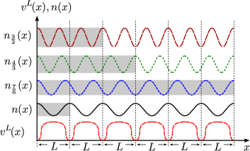
Figure 1: (color online)    Sketch of coordinate-scaled densities on unscaled external potential. Born-von Karman cells are denoted by the grey-shaded areas.

To cure this problem, we introduce the methodology of uniform coordinate and potential scaling (UCPS) under which we recover the differentiability of $E^{\Omega_{1}}_{\gamma,\scriptscriptstyle\rm UCS}$ at $\gamma=1$ essentially by scaling the external potential $\hat{V}^{\Omega_{1}}$. In detail, UCPS means the following: the electronic coordinate and wave function change according to UCS. Accordingly the external potential is scaled such that its periodicity coincides with the scaled wave function, $\hat{V}^{\Omega_{1}}\rightarrow\hat{V}^{\Omega_{\gamma}}$. The periodicity of a scaled wave function and the scaled external potential coincide and consequently Eq. (6) is a smooth function of $\gamma$. It is useful to translate the concept of scaling to operators. The identity

$$\left\langle\Psi^{\Omega_{1}}_{\gamma}\,\right|\hat{O}_{\gamma}\left|\,\Psi^{\Omega_{1}}_{\gamma}\right\rangle_{\Omega_{\gamma}} =\left\langle\Psi^{\Omega_{1}}_{1}\,\right|\hat{O}\left|\,\Psi^{\Omega_{1}}_{1}\right\rangle_{\Omega_{1}}$$ (10)

defines a scaled operator $\hat{O}_{\gamma}$, where we denote unscaled ($\gamma=1$) quantities explicitly by a subscript. The scaled operators for the kinetic and interelectronic interaction energy are simply related to their unscaled counterparts via

$$\hat{T}_{\gamma} =\hat{T}/\gamma^{2}, \hat{W}_{\gamma} =\hat{W}/\gamma\ .$$ (11)

The spatial kernel of the external potential operator scales according to $v^{\Omega_{\gamma}}_{\gamma}({{\bf r}})=v^{\Omega_{\gamma}}(\gamma\,{\bf r})$.

We now apply UCPS and obtain a well-defined expectation value

$$E^{\Omega_{1}}_{\gamma} =\left\langle\Psi^{\Omega_{1}}_{\gamma}\,\right|{\hat{H}}^{\Omega_{\gamma}}\left|\,\Psi^{\Omega_{1}}_{\gamma}\right\rangle_{\Omega_{\gamma}}=\left\langle\Psi^{\Omega_{1}}_{1}\,\right|\hat{H}_{1/\gamma}^{\Omega_{\gamma}}\left|\,\Psi^{\Omega_{1}}_{1}\right\rangle_{\Omega_{1}},$$ (12)

where the last equality follows from Eq. (10). Due to the scaling of the external potential the derivative with respect to $\gamma$ does now exist at $\gamma=1$, but, in contrast to the case of localized systems, it does not vanish in general. This is due to the fact that $\Psi_{\gamma}^{\Omega_{1}}$ is defined on a different volume $\Omega_{\gamma}$ for each $\gamma$ and therefore the extremum principle cannot be applied. However, we can relate the derivative with respect to the scale parameter to the pressure $P$ of the system:

$$-P=\lim_{\varepsilon\rightarrow 0}\frac{1}{\varepsilon}\left(E_{1}^{\Omega_{1}+\varepsilon}-E_{1}^{\Omega_{1}}\right)\,,$$ (13)

where $E_{1}^{\Omega_{1}+\varepsilon}=\left\langle\Psi_{1}^{\Omega_{1}+\varepsilon}\,\right|\hat{H}^{\Omega_{1}+\varepsilon}\left|\,\Psi_{1}^{\Omega_{1}+\varepsilon}\right\rangle_{\Omega_{1}+\varepsilon}$ and $E_{1}^{\Omega_{1}}=\left\langle\Psi_{1}^{\Omega_{1}}\,\right|\hat{H}^{\Omega_{1}}\left|\,\Psi_{1}^{\Omega_{1}}\right\rangle_{\Omega_{1}}$. Since $\Psi_{1}^{\Omega_{1}+\varepsilon}$ and $\Psi_{1}^{\Omega_{1}}$ are defined on different volumes, this complicates the use of perturbation theory. A way out of this dilemma is found by applying Eq. (10) to $E_{1}^{\Omega_{1}+\varepsilon}$ with the scale factor

$$\widetilde{\gamma} =\left[(\Omega_{1}+\varepsilon)/(\Omega_{1})\right]^{D}.$$ (14)

Then, $E_{1}^{\Omega_{1}+\varepsilon}$ can be calculated as the first order correction to $E_{1}^{\Omega_{1}}$ under the perturbation $\Delta\hat{H}=\hat{H}^{\Omega_{\widetilde{\gamma}}}_{\widetilde{\gamma}}-\hat{H}^{\Omega_{1}}_{1}$. Since we have ensured that the first order derivative with respect to $\gamma$ exists, we find

$$\left.\partial_{\gamma}E^{\Omega_{1}}_{\gamma}\right|_{\gamma=1} =-D\,\Omega_{1}\left.\partial_{\Omega}E^{\Omega}_{1}\right|_{\Omega=\Omega_{1}}\ .$$ (15)

Alternatively, this can be written as

$$\begin{split}&2T^{\Omega_{1}}+W^{\Omega_{1}}+\int_{\Omega_{1}}d^{D}r\ n^{\Omega_{1}}({{\bf r}})\,\partial_{\gamma}v^{\Omega_{\gamma}}({{\bf r}}/\gamma)|_{\gamma=1}\\ &=-D\,\Omega_{1}\,\partial_{\Omega}E_{1}^{\Omega}|_{\Omega=\Omega_{1}}\,,\end{split}$$ (16)

which reduces to Eq. (2) for Coulombic matter. Both Eqs. (15) and (16), relating the change of the energy under a change of volume with a change in the scale parameter, yield the most general expression for the VT. This is one of our main results.

We demonstrate the consistency of the VT for periodic systems that we just derived with an elementary example of a solid explicitly. Consider the simplified Kronig-Penney model Pedersen et al. (1991) – a one-dimensional lattice of Dirac delta functions of strength $\alpha$ separated by a distance $L$ – given by the Hamiltonian

$$H(x) =-\frac{1}{2}\partial^{2}_{x}-\frac{\alpha}{L}\sum_{\nu}\delta\left(x-L\left(\nu-1/2\right)\right)\ .$$ (17)

A simple solution for positive energies is $\phi(x)\propto\cos(qx/L)$, where $q$ is determined from $q=q\cos(q)-\alpha\sin(q)$. For a single particle in this state the energy is

$$E^{L}_{1} =q^{2}/(2L^{2})\ .$$ (18)

The expectation values of the scaled kinetic and potential energy are related to the unscaled quantities simply by

$$\left\langle\phi^{L}_{\gamma}\,\right|\hat{T}\left|\,\phi^{L}_{\gamma}\right\rangle_{L_{\gamma}} =\gamma^{2}\left\langle\phi^{L}_{1}\,\right|\hat{T}\left|\,\phi^{L}_{1}\right\rangle_{L}\,,$$ (19)

$$\left\langle\phi^{L}_{\gamma}\,\right|\hat{V}^{L_{\gamma}}\left|\,\phi_{\gamma}\right\rangle_{L_{\gamma}} =\gamma^{2}\left\langle\phi^{L}_{1}\,\right|\hat{V}^{L}\left|\,\phi^{L}_{1}\right\rangle_{L}\ .$$ (20)

Due to the specific form of the external potential there is a quadratic dependence on the scaling parameter relating the scaled and unscaled potential energy. Now we explicitly check Eq. (15). With Eqs. (18), (19), and (20), the left-hand side yields

$$\left.\partial_{\gamma}E^{L}_{\gamma}\right|_{\gamma=1}=q^{2}/L^{2}\ .$$ (21)

Using Eq. (18), the RHS of Eq. (15) is then simply shown to be identical to Eq. (21).

In the framework of DFT, as was mentioned before, only the VT for localized systems has been considered. Equipped with the new technique we are able to derive the exact properties of the XC functional valid for periodic systems. We apply Eq. (15) to an interacting and a noninteracting system (KS system) of the same density. Taking the difference of two VTs and thereby expressing the interelectronic interaction in terms of KS quantities, i.e., $W^{\Omega_{1}}=U^{\Omega_{1}}+E_{\scriptscriptstyle\rm XC}^{\Omega_{1}}-T_{\scriptscriptstyle\rm C}^{\Omega_{1}}$ yields:

$$\begin{split}&T_{\scriptscriptstyle\rm C}^{\Omega_{1}}+U^{\Omega_{1}}+E_{\scriptscriptstyle\rm XC}^{\Omega_{1}}+D\,\Omega_{1}\,\partial_{\Omega}\left.\left(E_{1}^{\Omega}-E_{\rm s}^{\Omega}\right)\right|_{\Omega=\Omega_{1}}=\\ &-\int_{\Omega_{1}}\!\!\!d^{D}r\ n^{\Omega_{1}}({{\bf r}})\partial_{\gamma}\left.\left[v^{\Omega_{\gamma}}\left(\frac{{{\bf r}}}{\gamma}\right)-v_{\rm s}^{\Omega_{\gamma}}\left(\frac{{{\bf r}}}{\gamma}\right)\right]\right|_{\gamma=1}\,,\end{split}$$ (22)

where $U^{\Omega_{1}}$ denotes the Hartree, $E_{\scriptscriptstyle\rm XC}^{\Omega_{1}}$ the XC, and $T_{\scriptscriptstyle\rm C}^{\Omega_{1}}=T^{\Omega_{1}}-T_{\rm s}^{\Omega_{1}}$ the kinetic correlation energies. The KS and external potential are scaled along the lines of Eq. (10) and

$$v_{\rm s}^{\Omega_{1}}({{\bf r}})-v^{\Omega_{1}}({{\bf r}})=v_{\scriptscriptstyle\rm XC}^{\Omega_{1}}({{\bf r}})+v_{\scriptscriptstyle\rm H}^{\Omega_{1}}({{\bf r}}),$$ (23)

where $v_{\scriptscriptstyle\rm XC}^{\Omega_{1}}({{\bf r}})=\delta E_{\scriptscriptstyle\rm XC}^{\Omega_{1}}/\delta n({{\bf r}})$ denotes the XC potential and $v_{\scriptscriptstyle\rm H}({{\bf r}})=\int_{\Omega_{\infty}}d^{D}r^{\prime}\ n^{\Omega_{1}}({{\bf r}}^{\prime})/|{{\bf r}}-{{\bf r}}^{\prime}|$ the Hartree potential. With Eq. (23) and using the fact that all terms containing Hartree and exchange contributions cancel each other, we obtain the following virial relation for the kinetic correlation energy:

$$\begin{split}T_{\scriptscriptstyle\rm C}^{\Omega_{1}}&=-E_{\scriptscriptstyle\rm C}^{\Omega_{1}}+\int_{\Omega_{1}}d^{D}r\ n^{\Omega_{1}}({{\bf r}})\,\partial_{\gamma}v_{\scriptscriptstyle\rm C}^{\Omega_{\gamma}}({{\bf r}}/\gamma)|_{\gamma=1}\\ &-D\Omega_{1}\partial_{\Omega}\left[E_{\scriptscriptstyle\rm C}^{\Omega}-\int_{\Omega}d^{D}r\ n^{\Omega}({{\bf r}})\,v_{\scriptscriptstyle\rm C}^{\Omega}({{\bf r}})\right]|_{\Omega=\Omega_{1}}\ .\end{split}$$ (24)

The analysis of the slowly varying limit of Eq. (24) sheds some light on the differences of the present work with the previous ones. For this, we need to use that $\partial_{\gamma}v_{\scriptscriptstyle\rm C}^{\Omega_{\gamma}}({{\bf r}}/\gamma)|_{\gamma=1}\approx\partial_{\gamma}v_{\scriptscriptstyle\rm C}^{\Omega_{\gamma}}({{\bf r}})|_{\gamma=1}=-D\,\Omega_{1}\partial_{\Omega}v_{\scriptscriptstyle\rm C}^{\Omega}({{\bf r}})|_{\Omega=\Omega_{1}}$, which is exact for the HEG, and approximately valid for systems with a slowly varying density. In this limit, Eq. (24) may be accordingly expressed as

$$\begin{split}T_{\scriptscriptstyle\rm C}^{\Omega_{1}}\approx&-E_{\scriptscriptstyle\rm C}^{\Omega_{1}}-D\Omega_{1}\partial_{\Omega}E_{\scriptscriptstyle\rm C}^{\Omega}|_{\Omega=\Omega_{1}}\\ &+D\Omega_{1}\left.\left[\partial_{\Omega}\int_{\Omega}d^{D}r\ n^{\Omega_{1}}({{\bf r}})\,v_{\scriptscriptstyle\rm C}^{\Omega_{1}}({{\bf r}})\right]\right|_{\Omega=\Omega_{1}}\\ &+D\Omega_{1}\int_{\Omega_{1}}d^{D}r\ \left[\partial_{\Omega}n^{\Omega}({{\bf r}})|_{\Omega=\Omega_{1}}\right]\,v_{\scriptscriptstyle\rm C}^{\Omega_{1}}({{\bf r}})\ .\end{split}$$ (25)

For the HEG case, $n^{\Omega}({{\bf r}})=n^{\Omega}=N/\Omega$, and $v_{\scriptscriptstyle\rm C}^{\Omega}({{\bf r}})=v_{\scriptscriptstyle\rm C}^{\Omega}=v_{\scriptscriptstyle\rm C}(n^{\Omega})$; the last two terms on the RHS cancel with each other, while the second term may be expressed as in Eq. (2), using that $\Omega_{1}=4\pi r_{s}^{3}/3N$. For the evaluation of Eq. (25) in the LDA, one needs to consider that $E_{\scriptscriptstyle\rm C}^{\Omega}=\int_{\Omega}d^{D}r\,n^{\Omega}({{\bf r}})\,\varepsilon_{\scriptscriptstyle\rm C}[n^{\Omega}({{\bf r}})]$, and that $v_{\scriptscriptstyle\rm C}^{\Omega}({{\bf r}})=v_{\scriptscriptstyle\rm C}[n^{\Omega}({{\bf r}})]$. Proceeding along the lines of Ref. Legrand and Perrot (2001), we obtain the following well-known expression of Levy and Perdew (LP)Levy and Perdew (1985),

$$T_{\scriptscriptstyle\rm C}^{\Omega_{1}}\approx-4\,E_{\scriptscriptstyle\rm C}^{\Omega_{1}}+3\int_{\Omega_{1}}d^{3}r\ n^{\Omega_{1}}({{\bf r}})\,v_{\scriptscriptstyle\rm C}[n^{\Omega_{1}}({{\bf r}})]\;.$$ (26)

Eq. (26), whose local version reads $t_{\scriptscriptstyle\rm C}[n^{\Omega_{1}}({{\bf r}})]=-4\,\varepsilon_{\scriptscriptstyle\rm C}[n^{\Omega_{1}}({{\bf r}})]+3\,v_{\scriptscriptstyle\rm C}[n^{\Omega_{1}}({{\bf r}})]$, has been obtained in Ref. Levy and Perdew (1985) restricting the analysis to the case of localized systems, where, as discussed above, the normalization volume can be taken as $\Omega_{\infty}$ and then is not affected by scaling. Here, proceeding from the extended or periodic scenario, we have arrived to the same result. This is however reasonable, since the distinction between a system as localized or extended becomes progressively less clear as the system approaches the truly slowly varying limit. Note however, that the HEG limit cannot be reached under the assumptions of Ref. Levy and Perdew (1985), while it is exactly reproduced by our general approach.

Table 1: Numerical values for the kinetic correlation energy $T_{\scriptscriptstyle\rm C}$ in Eq. (24), computed for a set of realistic periodic systemscom in LDA and GGA. All values are given in Rydbergs/formula unit. $\Delta T_{\scriptscriptstyle\rm C}$ is the difference between this exact form and the approximate one derived by Levy and Perdew (Eq. (26)) evaluated on LDA quantities (energies, densities, and potentials). The already excellent agreement further improves (see $\Delta T_{\scriptscriptstyle\rm C}^{*}$) by including GGA corrections on $v_{\scriptscriptstyle\rm C}$ using the PBE XC functional (this difference is of the same order of magnitude of the estimated numerical accuracy of the calculations and therefore should be read as zero).

	$T_{\scriptscriptstyle\rm C}$		$\Delta T_{\scriptscriptstyle\rm C}/10^{-2}$		$\Delta T_{\scriptscriptstyle\rm C}^{*}/10^{-5}$
pressure	–	200GPa	–	200GPa	–	200GPa
Diamond	12.65	13.83	-2.12	-1.49	8.46	11.2
LiF	10.99	14.14	-1.19	-1.53	8.20	10.5
Graphite	3.80	4.62	-0.99	-1.10	-0.31	-0.46
LiFeAs	4.65	4.78	-0.20	-0.29	3.36	3.41
Ar	4.62	5.56	-0.58	-0.83	4.17	5.01
PdH	9.78	10.49	-1.33	-1.83	26.3	27.6
NaCl	14.57	20.29	-1.13	-2.36	5.17	7.29

The expression in Eq. (24) for the kinetic correlation energy derived in this work is formally exact and equally valid for extended and localized systems, for both slowly and rapidly varying densities. We compare the exact expression in Eq. (24) with the LP simplified form given in Eq. (26) by computing their difference for a set of real crystals of different chemical properties at low and high pressurecom . In Tab. 1 we evaluate the difference between Eqs. (24) and (26) on LDA ($\Delta T_{\scriptscriptstyle\rm C}$) and GGA ($\Delta T_{\scriptscriptstyle\rm C}^{*}$) quantities (energies, densities, and potentials). As shown in Tab. 1, the difference within LDA is very small, of the order of $10^{-2}$ Ry per formula unit. This difference is hardly relevant for chemical application, and does not increase even when high pressure is applied. When we turn to the GGA results, the difference in $T_{\scriptscriptstyle\rm C}$ goes further down, by two orders of magnitude (below the estimated numerical error). This means that just by including the gradient corrections to $v_{\scriptscriptstyle\rm C}$ the LP formula gives essentially the exact $T_{\scriptscriptstyle\rm C}$. Note however, that according to Eq. (9) in Ref. Legrand and Perrot (2001), the correct GGA for the kinetic correlation energy has more contributions than just those obtained from replacing $E_{\scriptscriptstyle\rm C}$ and $v_{\scriptscriptstyle\rm C}$ by the corresponding GGA quantities in Eq. (26).

We note in passing that the very important adiabatic connection formulaParr and Yang (1989), which gives the XC energy functional as a coupling-constant integral of the coupling-constant dependent expectation value of the interelectronic interaction ($W$ in Eq.(1)), remains unchanged for periodic systems, since the adiabatic coupling-constant technique employed in its derivation does not change the periodicity of the density and Hamiltonian. This is consistent with the fact that the coupling-constant wave function may be expressed as $\Psi^{\Omega_{1}}_{\gamma}[n_{1/\gamma}]$, which does not leave the domain of the Hamiltonian.

Eq. (15) is valid not only for the ground state, but for all eigenstates $\Psi^{\Omega_{1}}_{i}$ of $\hat{H}^{\Omega_{1}}$. This enables us to derive corresponding versions of Eq. (15) for canonical and grand-canonical ensembles in the following.

Considering the canonical ensemble first, the equilibrium is defined as the state with minimal free energy $F^{\Omega_{1}}=E^{\Omega_{1}}-1/\beta S^{\Omega_{1}}$, where $S^{\Omega_{1}}$ is the entropy and $\beta=1/(k_{B}\tau)$ is a measure for the temperature $\tau$, $k_{B}$ being Boltzmann’s constant. A general quantum state is described by a statistical density operator $\hat{\Gamma}^{\Omega_{1}}$, a weighted sum of projection operators on the underlying Hilbert space $\hat{\Gamma}^{\Omega_{1}}=\sum_{i}w^{\Omega_{1}}_{i}|\,\Psi^{\Omega_{1}}_{i}\rangle\langle\Psi^{\Omega_{1}}_{i}\,|,\ (w^{\Omega_{1}}_{i}>0,\sum_{i}w^{\Omega_{1}}_{i}=1)$. The minimizing weights are then given by $w^{\Omega_{1}}_{i}=e^{-\beta E^{\Omega_{1}}_{i}}/Z$, where $E^{\Omega_{1}}_{i}$ is the i-th eigenvalue of $\hat{H}^{\Omega_{1}}$ and $Z$ is the normalization constant, i.e., the partition function. This, in connection with Eq. (12), leads to the following definition for the free energy in UCPS:

$$F_{\gamma}^{\Omega_{1}} =\sum_{i}\left(w^{\Omega_{1}}_{i}\langle\Psi^{\Omega_{1}}_{i\ \gamma}\,|\hat{H}^{\Omega_{\gamma}}|\,\Psi^{\Omega_{1}}_{i\ \gamma}\rangle+\ln(w^{\Omega_{1}}_{i})\right)$$ (27)

A coordinate scaling of the wave functions does not affect the weights $w^{\Omega_{1}}_{i}$ and therefore leaves the entropic contribution invariant. Furthermore, Eq. (27), by definition, is minimal for the particular choice of weights. The derivative with respect to volume therefore only yields contributions from the volume dependence of the energy expectation value. Combining these two findings we are lead to

$$\left.\partial_{\gamma}F^{\Omega_{1}}_{\gamma}\right|_{\gamma=1} =-D\,\Omega_{1}\left.\partial_{\Omega}F^{\Omega}_{1}\right|_{\Omega=\Omega_{1}},$$ (28)

which is the equivalent of Eq. (15) for canonical ensembles.

The same arguments can also be applied to the case of grand canonical ensembles and its main thermodynamic variable, the grand potential $\Phi^{\Omega_{1}}=E^{\Omega_{1}}-\mu N-1/\beta S^{\Omega_{1}}$, where the additional coupling to a particle bath is governed by the chemical potential $\mu$, $N$ being the particle number,

$$\left.\partial_{\gamma}\Phi^{\Omega_{1}}_{\gamma}\right|_{\gamma=1} =-D\,\Omega_{1}\left.\partial_{\Omega}\Phi^{\Omega}_{1}\right|_{\Omega=\Omega_{1}}.$$ (29)

In this work we present the theoretical formalism of uniform coordinate and potential scaling in order to tackle a long-standing problem in DFT: the formulation of a correct VT valid both for molecular (localized) systems and for infinite periodic solids. However, our numerical implementation and calculation for a set of realisitic periodic systems shows that corrections by our exact formulation are extremely small. And, hence, the localized form of the VT in the slowly-varying limit is sufficiently accurate for solid state applications. Still there could be exotic cases in which the corrections become relevant. Moreover, our scaling technique may find application in describing properties of extended periodic systems at finite temperature, such as phase transitions.

We acknowledge useful discussions with S. Pittalis. C.R.P. thanks CONICET for partial financial support and ANPCyT under grant number PICT-2012-0379.

References

• Hohenberg and Kohn (1964) P. Hohenberg and W. Kohn, Phys. Rev. 136, B864 (1964).
• Kohn and Sham (1965) W. Kohn and L. J. Sham, Phys. Rev. 140, A1133 (1965).
• Perdew et al. (1996) J. P. Perdew, K. Burke,  and M. Ernzerhof, Phys. Rev. Lett. 77, 3865 (1996)ibid. 78, 1396(E) (1997).
• Mermin (1965) N. D. Mermin, Phys. Rev. 137, A1441 (1965).
• Pittalis et al. (2011) S. Pittalis, C. R. Proetto, A. Floris, A. Sanna, C. Bersier, K. Burke,  and E. K. U. Gross, Phys. Rev. Lett. 107, 163001 (2011).
• Levy and Perdew (1985) M. Levy and J. P. Perdew, Phys. Rev. A 32, 2010 (1985).
• Dreizler and Gross (1990) R. M. Dreizler and E. K. U. Gross, Density Functional Theory: An Approach to the Quantum Many-Body Problem (Springer–Verlag, 1990).
• Marc and McMillan (2007) G. Marc and W. G. McMillan, “The virial theorem,” in Advances in Chemical Physics (John Wiley and Sons, Inc., 2007) pp. 209–361.
• Note (1) For brevity we use a short-hand notation for derivatives, such as $\partial_{\Omega}=\partial/\partial\Omega$.
• Slater (1933) J. C. Slater, J. Chem. Phys. 1, 687 (1933).
• Cottrell and Paterson (1951) T. Cottrell and S. Paterson, Phil. Mag. Series 7 42, 391 (1951).
• Argyres (1967) P. N. Argyres, Phys. Rev. 154, 410 (1967).
• Ziesche (1980) P. Ziesche, J. Phys. C: Solid State Physics 13, 3625 (1980).
• Fernandez and Castro (1982) F. M. Fernandez and E. A. Castro, Int. J. Quantum Chem. 21, 741 (1982).
• Bobrov et al. (2010) V. B. Bobrov, S. A. Trigger, G. J. F. van Heijst,  and P. P. J. M. Schram, Phys. Rev. E 82, 010102 (2010).
• Esteve et al. (2012) J. G. Esteve, F. Falceto,  and P. R. Giri, Phys. Rev. A 85, 022104 (2012).
• Resta (1994) R. Resta, Rev. Mod. Phys. 66, 899 (1994).
• Note (2) Inserting the correctly scaled external potential $v^{L_{\gamma}}(x)$ into Eq. (6) and taking the limit $M\to\infty$, it can be proven that the discontinuity in the external potential energy per unit cell disappears.
• Pedersen et al. (1991) F. B. Pedersen, G. T. Einevoll,  and P. C. Hemmer, Phys. Rev. B 44, 5470 (1991).
• Legrand and Perrot (2001) P. Legrand and F. Perrot, J. Phys.: Condens. Matter 13, 287 (2001).
• (21) All systems are computed at the LDA relaxed structure. The numerical error in $T_{\scriptscriptstyle\rm C}$ due to the numerical derivatives with respect to $\gamma$ has been estimated to be of the order of $10^{-4}$ Ry. Calculations have been done in the norm conserving pseudopotential approximation within the ESPRESSO planewave codeGiannozzi et al. (2009). The planewave expansion of the Block orbitals has been cut at 100 Ry or above.
• Parr and Yang (1989) R. G. Parr and W. Yang, Density Functional Theory of Atoms and Molecules (Oxford University Press, 1989).
• Giannozzi et al. (2009) P. Giannozzi, S. Baroni, N. Bonini, M. Calandra, R. Car, C. Cavazzoni, D. Ceresoli, G. L. Chiarotti, M. Cococcioni, I. Dabo, A. Dal Corso, S. de Gironcoli, S. Fabris, G. Fratesi, R. Gebauer, U. Gerstmann, C. Gougoussis, A. Kokalj, M. Lazzeri, L. Martin-Samos, N. Marzari, F. Mauri, R. Mazzarello, S. Paolini, A. Pasquarello, L. Paulatto, C. Sbraccia, S. Scandolo, G. Sclauzero, A. P. Seitsonen, A. Smogunov, P. Umari,  and R. M. Wentzcovitch, J. Phys.: Condens. Matter 21, 395502 (2009).