High-resolution observations of active region moss and its dynamics
Abstract
The High resolution Coronal Imager (Hi-C) has provided the sharpest view of the EUV corona to date. In this paper we exploit its impressive resolving power to provide the first analysis of the fine-scale structure of moss in an active region. The data reveal that the moss is made up of a collection of fine threads, that have widths with a mean and standard deviation of km (Full Width Half Maximum). The brightest moss emission is located at the visible head of the fine-scale structure and the fine structure appears to extend into the lower solar atmosphere. The emission decreases along the features implying the lower sections are most likely dominated by cooler transition region plasma. These threads appear to be the cool, lower legs of the hot loops. In addition, the increased resolution allows for the first direct observation of physical displacements of the moss fine-structure in a direction transverse to its central axis. Some of these transverse displacements demonstrate periodic behaviour, which we interpret as a signature of kink (Alfvénic) waves. Measurements of the properties of the transverse motions are made and the wave motions have means and standard deviations of km for the transverse displacement amplitude, s for the period and km/s for the velocity amplitude. The presence of waves in the transition region of hot loops could have important implications for the heating of active regions.
1 Introduction
One of the fundamental and persistent problems in astrophysics is the puzzle of how the solar corona is heated. There has been a wide range of scenarios proposed to explain the observed high temperatures ( MK), e.g., magnetic reconnection (nanoflares - Parker 1988), magnetohydrodynamic (MHD) waves (Cranmer et al. 2007) and type-II spicules (De Pontieu et al. 2011) - although it is not necessary that each of these are exclusive. It is generally accepted that the contributing processes are likely to occur on small spatial and temporal scales.
The High resolution Coronal Imager (Hi-C) (Kobayashi et al. 2014) provided a unique view of the EUV corona and, despite the relatively short lifetime of the mission ( s), has allowed for a number of insights into small-scale coronal features (Brooks et al. 2013; Peter et al. 2013; Alexander et al. 2013). In particular, Hi-C allowed for a detailed study of the moss regions (Testa et al. 2013; Winebarger et al. 2013), i.e., the upper Transition Region emission of high pressure loops in active regions. The moss appears as a reticulated pattern of bright emission in EUV images, with large-scale structuring on spatial scales of 2-3 Mm, with an apparent vertical extent of Mm (Berger et al. 1999; Fletcher & de Pontieu 1999). The bright emission is punctuated with patches of low emission (‘dark inclusions’) and, in general, the regions of low emission show a correlation with spicules observed in H wings (De Pontieu et al. 2003). However, previous instruments have not had the ability to resolve fine-scale structure in either the bright or dark regions.
Moss has been the focus of much interest (e.g., Tripathi et al. 2010; Brooks et al. 2010) since it was proposed that the moss emission scales well with loop pressure (Martens et al. 2000), enabling variations in the moss to provide a diagnostic tool for the study of coronal heating mechanisms. Moreover, observations have revealed that moss emission varies little over extended time periods (e.g., Antiochos et al. 2003; Brooks & Warren 2009), implying that the heating must be quasi-steady in nature and dominated by continuous high-frequency heating events. This scenario has support from reports of high-frequency intensity variations in the moss, observed with the high spatial and temporal resolution of Hi-C (Testa et al. 2013). On the other hand, time variability of the moss could well be due to motions of the magnetic field rather than a direct signature of heating. This was suggested by Antiochos et al. (2003) and Brooks & Warren (2009) in relation to variability on long time-scales, but could also apply to the variability observed on shorter time-scales.
In recent years, the role of MHD waves in heating has been brought to the forefront of the field due to observations of ubiquitous kink (Alfvénic) wave behaviour throughout the chromosphere (De Pontieu et al. 2007b; Kuridze et al. 2012; Morton et al. 2012a, 2013a) and corona (Tomczyk et al. 2007; van Doorsselaere et al. 2007; Erdélyi & Taroyan 2008; McIntosh et al. 2011). In particular, the observed chromospheric waves have an estimated wave energy flux in excess of that needed to meet the heating requirements of the active corona. However, current observations of EUV coronal loops reveal that the kink wave energy flux in the corona is generally too small to contribute to heating in the coronal volume (Tomczyk et al. 2007; McIntosh et al. 2011; Morton & McLaughlin 2013). This lack of observed wave energy may be in part due to wave reflection at the Transition Region (e.g., Okamoto & De Pontieu 2011) or the waves may have been significantly damped/undergone mode conversion before reaching the observable EUV corona (e.g., Verth et al. 2010; Morton et al. 2014). To date, it has not been possible to carry out similar wave studies for warm/hot loops due to a combination of low spatial resolution, low signal-to-noise and the increased ‘fuzziness’ of warm loops in imaging observations (e.g., Brickhouse & Schmelz 2006).
Hi-C has provided images of resolved fine-scale structure in coronal loops and while studies have exploited the high spatial and temporal resolution of Hi-C to investigate the temporal variations in moss regions, the spatial structure has not yet been examined. Here we provide the first analysis of the fine-scale spatial structure of the moss regions. It is found that the bright moss is located at the upper end of elongated fine-structure that has spatial scales of a few 100 km, similar to those observed in the chromospheric fine- structure (e.g., Morton et al. 2012a; Antolin & Rouppe van der Voort 2012; Pereira et al. 2012) and EUV loops (e.g., Brooks et al. 2012, 2013; Peter et al. 2013). The fine-structure appears to be the lower (upper chromosphere/lower Transition Region) legs of the hot loops typically seen in soft X-rays. The ability to resolve the fine-scale structure associated with the moss also allows for the first imaging observations of transverse displacements of the structures. In particular, periodic transverse displacement of the fine-scale structure is observed and interpreted in terms of the kink (Alfvénic) mode. Measurements demonstrate the waves have periods and amplitudes similar to or smaller than those found previously in fibrils and spicules, respectively (e.g., Okamoto & De Pontieu 2011; Pereira et al. 2012; Kuridze et al. 2012; Morton et al. 2012a, 2013a).
2 Observations and data reduction
Details of the Hi-C observations can be found in, e.g., Morton & McLaughlin (2013). We note here that the cadence of the data is on average 5.57 s, a correction from the cadence given in Morton & McLaughlin (2013). The data was processed and aligned by the Hi-C science team, however, we note that the data still displayed visible shifts and additional alignment was performed using cross-correlation, achieving sub-pixel accuracy on the frame-to-frame alignment. The data are missing a frame between 18:54:28-18:54:40 UT (time stamp corrected), therefore we used interpolation to create the missing frame and provide a constant sampling rate for wave studies. The first seven frames of the Hi-C data are subject to viewing distortions due to rocket jitter and prove inadequate for rigid alignment; hence, they are not used for analysis. In addition, we compare the Hi-C data to data from the Solar Dynamic Observatory (SDO) Atmospheric Imaging Assembly (AIA) (Lemen et al. 2011), which is prepared using the standard routines. Alignment between Hi-C and SDO images is performed by degrading the spatial sampling of the Hi-C data to match that of SDO and using cross-correlation.
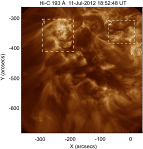
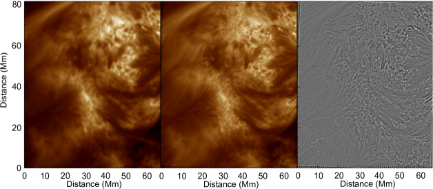
The Hi-C bandpass is centred close to 193 Å, which has strong contributions from Fe XII that has a peak formation temperature close to MK and is ideal for observing coronal features. As reported in Morton & McLaughlin (2013) and Brooks et al. (2013), the images show apparently resolved coronal loops (Figure 1). In addition, it is evident that there exists fine structure in the moss regions. It is these features that are the subject of the following investigation.
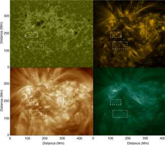
Figure 1 shows the Hi-C field of view and the brightest moss regions are indicated by the dashed boxes. Testa et al. (2013) demonstrated that these regions lie at the foot-points of the hottest coronal loops in the active region, which have significant X-ray emission observed in co-temporal observations from Hinode X-Ray Telescope (XRT - Golub et al. 2007). These hot loops are also observed in Figure 1 in 94 Å (Fe XVIII). While these are likely the hottest loops in the region, we argue that there are other hot (or at least warm MK) loops in the Hi-C field of view. In Figure 1 we identify two additional regions that we suggest can be classified as moss. Firstly, bright patches in 1600 Å (continuum plus C IV) images provide a good proxy for identifying magnetic elements and both the highlighted regions show enhanced, plage-like emission. Secondly, these regions in 171 Å (Fe IX) images show the reticulated emission typically associated with moss, with no evident coronal loop structures originating in the regions. This is in contrast to 193 Å, which demonstrates the presence of very fine-scale, diffuse loops that are apparently rooted in the identified regions. In the 94 Å bandpass, these diffuse fine-scale loops appear as a haze of emission, with the emission above the bright ‘moss’ having a marginally greater intensity. The fuzziness of the loops would suggest they are MK (Reale et al. 2011), although the identification of any fine-structure in the 94 Å channel is restricted due to the lower signal-to-noise, i.e., compared to the 193 Å channel. In XRT images, region 3 has faint emission (compared to the hot loops) while region 4 lies outside the XRT field of view (see Figure 1 of Testa et al. 2013).
Taking into account the thermal responses of the AIA channels, the lack of emission for the diffuse fine-scale loops in the 171 Å channel and the presence of emission in 193 Å and 94 Å channels, this suggest the moss regions are foot-points of warm or hot loops ( MK). The temperature of these threads requires there to be enhanced pressure at the loop foot-points, which in turn leads to enhanced emission in the Transition Region. The weaker emission of the moss (relative to the bright moss regions 1 and 2) suggests that the pressure at the Transition Region of these loops is lower or the loop filling factor is less than the hottest loops observed in 94 Å (Martens et al. 2000).
3 Results
3.1 Fine-scale structure of the moss
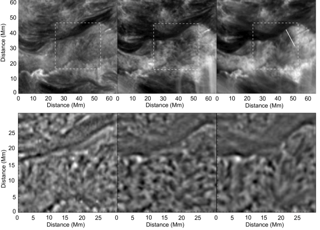
We begin by providing a view of moss as it is observed with AIA. Figure 2 (top row) shows a close up of region 2 in AIA 304 Å, 171 Å and 193 Å bandpasses. The AIA images suggest that small-scale structuring in the moss regions is present but it is clearly unresolved. In Figure 3, we display an image taken with Hi-C that focuses on the same patch of the moss as shown in the bottom row of Figure 2. The fine structuring is now evident appearing as threads, but the threads visibility is clearer after passing the data through an unsharp-mask routine. The Hi-C data reveals that the fine structures are connected to the bright moss and appear to be an extension of the bright moss into the lower solar atmosphere.
These fine threads are visible in the dark inclusions, hence have reduced emission relative to the bright moss. Figure 6 shows the intensity profiles of seven typical groups of the fine-structure (displayed in Figure 5), where the profile is parallel to the axis and averaged over the group (groups consisting of 15-20 features). The intensity along the structures is found to steadily decrease from the bright moss into the dark inclusions. Previous limb observations with TRACE data demonstrated that moss has an apparent vertical extent on the order of km (Martens et al. 2000). The fine-scale structures seen here appear to be have similar vertical scales (with some more extended moss regions), although it is difficult to locate where individual threads end/begin (see, Figures 3 and 4).
The particular dark inclusion shown in Figure 3 is a gap between two patches of bright moss. Each patch of moss can be seen to be composed of groups of fine-scale structure and the groups are inclined at different orientations. The variation in inclination of individual moss patches has been noted previously by Katsukawa & Tsuneta (2005).
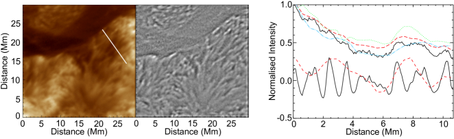
In Figure 4 we show an example of a larger patch of moss corresponding to region 1. On viewing the unsharp masked Hi-C image, the wealth of fine-scale structure in the moss regions is evident. The moss region centred at (30,30) provides a clear demonstration of the extension of the fine structure. The bright moss emission is at the head of the fine-scale structures, which extend off to the left hand side, gradually fading and becoming indistinguishable from the background emission. The formation of the structures is reminiscent of a chain of mountains, with the fine structure forming the sides of the mountain, meeting in the middle with the bright moss emission as the peaks. This formation is often seen in active regions imaged with H (e.g., De Pontieu et al. 2003, 2007a; Kuridze et al. 2011), where the chromospheric structures tend towards a central location, occasionally having enhanced emission.
The difference between the Hi-C and the AIA view of the moss is elucidated in Figure 3. Taking a cross-cut perpendicular to the fine structure and plotting the intensity reveals that the individual strands are unresolved by AIA, while Hi-C shows peaks in emission related to the fine structure. Again, the fine structure is better visualised by comparing the intensity profiles from unsharp masked images (i.e. after subtracting the local mean intensity) for the same cross-cuts for Hi-C and AIA.
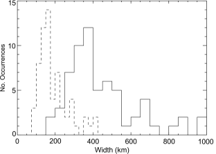
In order to reveal the typical scale of the fine structures, we select features from each of the identified moss regions and measure their widths in the Hi-C data. The fine structure in unsharp masked images are fitted with a combination of a Gaussian function and a linear function. In Figure 7 we display both the values of the Gaussian and the Full-Width-Half-Maximum () values. The measured widths are comparable to the results obtained for coronal loops (e.g., Brooks et al. 2013) and for chromospheric structures (e.g., De Pontieu et al. 2007a; Morton et al. 2012a).

3.2 Dynamics of the moss
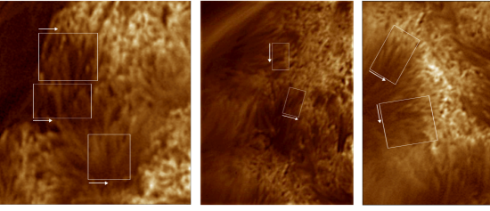
Being able to resolve the fine structure now allows for the examination of the dynamic behaviour in the moss regions. The data reveal that the fine-structure of the moss exhibits motions in the direction transverse to its axis, some of which demonstrate periodic behaviour. Examples of the observed transverse displacements are displayed in Figure 8.
General information about the techniques used in this paper to track and measure the transverse displacements are described in detail in Morton & McLaughlin (2013). However, we have advanced our analysis techniques and provide a brief description of them here.
Due to the high read noise of Hi-C, we apply a filtering technique to each frame to suppress the the highest frequency spatial components. First, an Atrous filter is applied to each frame which extracts high frequency spatial components. The resulting high-frequency images still show signs of distinct structure. We then unsharp mask the high frequency component with a 3 by 3 boxcar function. This allows us to isolate a significant portion of the noise while minimising any potential signal loss. In theory, this procedure should separate the noise with a spatial variation less than 3 pixels. The diffraction limited seeing of Hi-C is (around 3 pixels - Kobayashi et al. 2014); hence, the spatial variations are below the diffraction limit. The residual noise image shows a flat power spectral density and suggests uncorrelated noise (as also found in Kobayashi et al. 2014). The noise image is then subtracted from the original data. This technique reduces the amount of signal loss compared to that used in Morton & McLaughlin (2013), while still significantly improving the visibility of small-scale features in images by the removal of the majority of the read noise.
The data is then subject to unsharp masking and cross-cuts are taken perpendicular to features of interest and time-distance diagrams are created. The time-distance diagrams are generated by averaging the intensities over two neighbouring cross-cuts. The time-distance diagrams are then smoothed in space and time using a 3 by 3 pixel box-car function to suppress some of the additional large amplitude noise that arises from frame-to-frame variations in intensity levels. This aids the feature tracking routine that is then employed (e.g., Morton et al. 2013a), where a Gaussian function is fitted to the cross-sectional flux profile of each feature. The fit is supplied with the associated errors in data number, which are calculated using the formulae given in Morton & McLaughlin (2013) and divided by a factor of to account for the averaging over two neighbouring cross-cuts.
We focus on measuring transverse motions that display potential evidence for periodicity. The motions are fit with a combination of a sinusoidal function and a linear function (e.g. Morton & McLaughlin 2013). Upon testing the wave fitting routine on example data, the routine was able to detect periodic displacement amplitudes on the order of pixel (i.e. peak-to-peak displacement of pixel) for a signal-to-noise ratio of or greater. For the fine-structure observed in the moss regions, the signal-to-noise is . When fitting the transverse displacements, we require a minimum of of a cycle for it to be considered a potential signature of periodic behaviour. The selection of of a cycle is used since it ensures that the motion is observed at least in two directions and also allows for the peak-to-peak amplitude to be measured.
From the time-distance diagrams it is possible to measure the transverse displacement amplitude () and the period () of the waves. The velocity amplitude, , and its associated error can be calculated from these two quantities,
| (1) |
where is the error of the quantity .
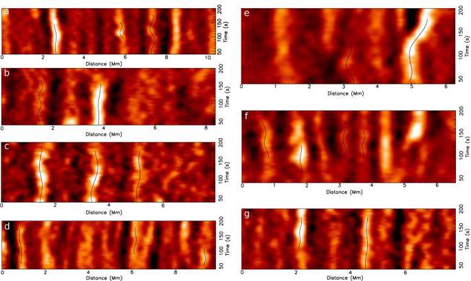
In the identified moss regions, we find 73 measurable examples of transverse displacements that demonstrate evidence for periodicity. A complete list of the measurements of , and are given in Table 1 along with the duration of each signal. Typical examples of time-distance diagrams are shown in Figure 8, with the associated measured data points and sinusoidal fits given in Figure 9. The majority of the measured transverse displacements show at least one cycle and typically only motions with periods longer than s show less than a whole period. Figure 10 gives the histograms for the measured transverse displacements, which have means and standard deviations of km for the transverse displacement amplitude, s for the period and km/s for the velocity amplitude. In addition to the periodic transverse displacements, some of the threads also display evidence for transverse motions that occur over longer time-scales. These motions cause the thread to appear to drift from its original position in the time distance diagram. This motion can also be superimposed with the periodic motions, as evidenced in e.g., Figure 9 b.2, e.2, g.3.

4 Discussion and conclusions
Moss regions observed in EUV passbands are thought to be the high pressure Transition Region of hot coronal loops. The fine-scale structuring of cooler ( 2 MK) coronal loops has been evident from measurements in EUV images (e.g., Watko & Klimchuk 2000; Brooks et al. 2012, 2013). Earlier observations from TRACE, EIT and Yohkoh suggested that loop widths may increase with temperature (Schrijver 2007), although this could be related to the lower spatial resolution of these previous missions. On the other hand, the observed width increase may be related to an increasing ‘fuzziness’ of loops with increasing temperature (Brickhouse & Schmelz 2006; Tripathi et al. 2009). However, there is a suggestion that the observed fuzziness decreases for passbands sensitive to temperatures greater than 3 MK (Guarrasi et al. 2010) and is apparently confirmed by SDO observations (Reale et al. 2011) although no measurements of individual loop widths are given. This would suggest that the hotter loops are structured on similar scales to the EUV loops.
4.1 Spatial scales of moss features
The increased resolution of Hi-C allows the fine-scale magnetic structure to be resolved in moss regions. The fine-scale structure is most evident in the dark inclusions accompanying the bright moss emission. The patches of bright moss emission correspond to the Transition Region of a collection of closely packed loop legs and the close proximity of the loops obscure the lower-altitude portion of the loop leg. When neighbouring groups of loops have different inclinations, a gap appears in the moss (i.e., a dark inclusion) and elongated fine-scale structure, corresponding to the lower-altitude portion of the loop leg, becomes visible (e.g., Figure 2). Similar structures are seen at the edges of moss regions when there are no neighbouring loops to obscure the view (Figure 4). The resolved features have measured widths similar to fine-scale structure in the EUV corona (Brooks et al. 2013).
It is interesting to note that the mean width ( km, FWHM km) of the structures measured here is larger than those obtained for dynamic fibrils (De Pontieu et al. 2007a - measured total width - km) and quiet Sun fibrils (Morton et al. 2012a - km, FHWM km) and smaller than those measured for coronal loops with Hi-C (Brooks et al. 2013 - km, FWHM km), which hints at magnetic flux-tube expansion between the chromosphere and corona. However, the given values are comparable within . In addition, direct comparisons between the results from different instruments is complicated by a number of factors. Firstly, the lower spatial resolution of Hi-C, compared to ROSA, may influence the distribution of the flux tubes widths measured here. Secondly, the measured width is not equal to the actual diameter of the structure, with a complex relationship existing between measured and physical loop widths dependent upon instrument characteristics (López Fuentes et al. 2006; Brooks et al. 2012, 2013). Finally, for all cases, i.e., chromospheric, Transition Region, and coronal magnetic structures, measurements are from small sample numbers. The combination of these factors limit the conclusions that can be drawn at this time regarding expansion.
4.2 Temperature regime of the fine-structure
The fine-structure has less emission than the bright moss, indicating the features contain plasma that is cooler than the bright moss and likely constitute the lower Transition Region/upper chromospheric sections of the hot loops. Let us consider the line intensity of coronal plasma,
where is the contribution function, the temperature, the electron density. As the fainter emission appears to form in the lower extension of the moss, it is expected that should be larger in the lower atmosphere (e.g. compare electron densities from the model P chromosphere of Fontenla et al. 2007 to measurements of moss densities - Tripathi et al. 2010). The increase in means that the contribution function must decrease if intensity is to decrease (as demonstrated in Figure 6), hence, the temperature of the plasma is decreasing. The intensity decreases at a steady rate (i.e. no sharp drop in intensity is observed) along the fine-structure from the bright moss, implying a similarly steady decrease in temperature. However, the plasma must be hot enough to contribute to the Å passband so must have a temperature greater than MK. The ability of Hi-C to resolve the structure in the dark inclusions and measure their faint emission is due to the larger effective area of Hi-C along with the increased resolution, when compared to the AIA 193 Å channel.
De Pontieu et al. (1999) noted that features in the dark inclusions in the moss can be relatively well correlated with absorption features observed in H, i.e., dynamic fibrils. Hi-C reveals dark striations are present amongst the faint emission, which may be the signatures of chromospheric material reaching high into the lower corona and absorbing/blocking the hotter Transition Region emission (De Pontieu et al. 2009). It may also be argued that the faint emission features in the dark inclusions are composed of cool, chromospheric plasma, which may be visible due to partial absorption of EUV radiation or scattered light. This may be true for the lowest section of the features but seems unlikely for the upper sections given the gradual decrease in intensity along the structures. Additionally, it would appear unlikely that the majority of these features are the upper atmospheric extensions of dynamic fibrils. This is due to the clear morphological differences between the sparsely populated jets seen in H (e.g., De Pontieu et al. 2007a) and the relatively dense population of features we observe with Hi-C.

4.3 Transverse motions - signatures of kink waves
The Hi-C data also reveals the transverse displacement of the moss fine structure. The observed displacements are of the fine-scale faint emission features that lie within the dark inclusions (see, Figures 2 and 3). The ability to measure transverse displacements in the dark inclusions is limited in part due to the low S/N levels in these regions and partially due to the small displacements ( km) the features undergo. This latter point is clear when considering the relative errors obtained for the smallest displacements in Table 1.
Due to some of the transverse motions displaying evidence for periodic behaviour, we interpret the observed motions as the kink (Alfvénic) wave. The presence of waves in the moss has been conjectured (Antiochos et al. 2003; Brooks & Warren 2009) and it is thought that the waves are the cause of some of the observed variability in the cores of the active region moss rather than heating events. We recall here that Berger et al. (1999) noted they observed the interaction of dynamic fibrils with the EUV moss, which occasionally pushed the moss elements aside. However, we suggest that the periodicity demonstrated by the motions reported here is a key indicator of wave behaviour, rather than the interaction of the dynamic fibrils with the EUV moss. Additionally, we do not see evidence for this interaction in the Hi-C data, although its likely that further high resolution coronal observations with co-temporal chromospheric data are required to observe such an interaction.
4.4 Insights into wave propagation through the atmosphere
The observation of the periodic transverse displacements in the moss features may suggests that kink (Alfvénic) waves can propagate into the Transition Region from the chromosphere. There is still an open question related to the fraction of Alfvénic wave energy, generated in the lower solar atmosphere, that is able to reach the corona. It has been suggested that a significant fraction of the energy is reflected at the Transition Region due to steep density gradients, with evidence from quiet Sun chromospheric observations suggesting around of the waves are reflected (Okamoto & De Pontieu 2011; Kuridze et al. 2013). The high pressure nature of the hot loops may reduce the sharpness of density gradient in the Transition Region (see, e.g. simulations of hot loops - Serio et al. 1981; Reale 2010) and allow waves to propagate more freely from the chromosphere to the corona.
If we assume that the observed transverse displacements can be interpreted in terms of kink waves, an estimate of the difference in energy, , and Poynting flux, , between the chromospheric and Transition Region waves can be made. To make this estimate we use the formulae for integrated energy and Poynting flux from Goossens et al. (2013). In deriving these formulae, Goossens et al. (2013) assume the wave-guide is a cylindrical, pressure-less, over dense flux tube. These assumptions are applicable to the fine-scale features we observe in the Hi-C images and also to dynamic fibrils in the chromosphere. Both features are likely low- plasmas, where , hence, can be considered pressure-less analytically. Additionally, the kink mode is known to be highly incompressible in the long wavelength limit (Goossens et al. 2009), so neglecting pressure will have little influence on the wave energy calculation. Further, the fine-scale features seen in Hi-C appear to be the lower atmospheric extension of the bright moss, hence, they will also have a high pressure and a greater density than the ambient coronal plasma in which they reside. Dynamic fibrils are jets of chromospheric plasma into the upper atmosphere, so are also over dense compared to the ambient plasma.
The ratio of Transition Region to chromospheric wave energy and Poynting flux is then
| (2) | |||||
| (3) |
Here, is the density and is the radius of the flux tube. The subscript TR and c correspond to Transition Region and chromosphere, respectively. The given ratios will likely be best described using frequency dependent functions. This is because damping mechanisms and reflection alter the wave amplitude and tend to show frequency dependent behaviour (e.g., Verth et al. 2010, Morton et al. 2014). At present we have to ignore such complications due to a lack of information and have used the mean value of the velocity amplitude measured here, km/s. To the best of our knowledge, there are no measurements of transverse displacements in dynamic fibrils to provide direct comparison too. However, the measured properties of the transverse displacements are similar to those measured in active region fibrils ( km/s; Morton et al. 2014), while the values are smaller than those reported for active region spicules (type-I - km/s; Pereira et al. 2012). We choose to use the values from active region fibrils ( km/s), to provide an upper limit for the energy transmission. It is clear that using active region spicules values of velocity amplitude ( km/s) would lead to much smaller ratios.
In addition, we have used cm-3 (e.g. Tripathi et al. 2010; Winebarger et al. 2011), cm-3 (Fontenla et al. 2007 - Model P), km, km (De Pontieu et al. 2007a) and characteristic values of the propagation speed of waves in the chromosphere ( km s-1 - Okamoto & De Pontieu 2011, Morton et al. 2012a) and Transition Region ( km s-1 - McIntosh et al. 2011) are used.
The estimates reveal that the Transition Region Poynting flux carried by waves is potentially smaller than that in the chromosphere. However, the overall wave energy has decreased by .
Moreover, the measured velocity amplitudes of the waves here are greater than those typically reported in observations of coronal kink waves in active regions ( km/s - Tomczyk et al. 2007; Erdélyi & Taroyan 2008; van Doorsselaere et al. 2008; Tian et al. 2012; Morton & McLaughlin 2013), which implies that kink waves are more energetic in the lower solar atmosphere compared to the active corona. McIntosh et al. (2011) and Morton & McLaughlin (2013) both present evidence for larger velocity amplitude ( km/s) transverse motions in the corona (unrelated to excitation by flare blast waves). However, as demonstrated in Morton & McLaughlin (2013), it does not appear as if these larger amplitude motions are ubiquitous throughout the active corona. We suggested that observed transverse displacements with large velocity amplitudes are related to significant energy releases in individual loop systems, e.g. via magnetic reconnection, and not continuously driven.
These estimates suggest that the majority of observed kink wave energy in the chromosphere is unable to reach the corona, however, they do not rule out waves as contributing to the heating budget of hot loops. The estimates suggest if waves are to play a role in active region heating then the energy deposition is likely to be localised in the chromosphere. Alternatively, the kink wave energy may have been converted to torsional motions of the fine-structure through mode-coupling via resonant absorption (e.g., Terradas et al. 2010; Pascoe et al. 2011). Similar findings are found for waves in quiet regions in Morton et al. (2014). The continuous driving of waves via granular or turbulent motions (e.g., van Ballegooijen et al. 2011) could provide the required quasi-steady heating mechanism in active regions. On the other hand, the observed waves could be the by-product of small-scale magnetic reconnection events, i.e., the classic nano-flares. It is well known from simulations of large-scale reconnection events that a fraction of the energy released is converted to wave energy (Yokoyama & Shibata 1996). The results presented here are a preliminary investigation into waves in the Transition Region but they point towards the need for extended statistical studies of wave propagation from the chromosphere to the corona. Such further study will be required to provide a clear and unequivocal picture of wave propagation through the atmosphere.
References
- Alexander et al. (2013) Alexander, C. E., Walsh, R. W., Régnier, S., et al. 2013, ApJ, 775, L32
- Antiochos et al. (2003) Antiochos, S. K., Karpen, J. T., DeLuca, E. E., Golub, L., & Hamilton, P. 2003, ApJ, 590, 547
- Antolin & Rouppe van der Voort (2012) Antolin, P. & Rouppe van der Voort, L. 2012, ApJ, 745, 152
- Berger et al. (1999) Berger, T. E., de Pontieu, B., Schrijver, C. J., & Title, A. M. 1999, ApJ, 519, L97
- Brickhouse & Schmelz (2006) Brickhouse, N. S. & Schmelz, J. T. 2006, ApJ, 636, L53
- Brooks & Warren (2009) Brooks, D. H. & Warren, H. P. 2009, ApJ, 703, L10
- Brooks et al. (2012) Brooks, D. H., Warren, H. P., & Ugarte-Urra, I. 2012, ApJ, 755, L33
- Brooks et al. (2013) Brooks, D. H., Warren, H. P., Ugarte-Urra, I., & Winebarger, A. R. 2013, ApJ, 772, L19
- Brooks et al. (2010) Brooks, D. H., Warren, H. P., & Winebarger, A. R. 2010, ApJ, 720, 1380
- Cranmer et al. (2007) Cranmer, S. R., van Ballegooijen, A. A., & Edgar, R. J. 2007, ApJS, 171, 520
- De Pontieu et al. (1999) De Pontieu, B., Berger, T. E., Schrijver, C. J., & Title, A. M. 1999, Sol. Phys., 190, 419-435
- De Pontieu et al. (2003) De Pontieu, B., Tarbell, T., & Erdélyi, R. 2003, ApJ, 590, 502
- De Pontieu et al. (2007b) De Pontieu, B., McIntosh, S. W., Carlsson, M., et al. 2007b, Science, 318, 1574
- De Pontieu et al. (2007a) De Pontieu, B., Hansteen, V. H., Rouppe van der Voort, L., van Noort, M., & Carlsson, M. 2007a, ApJ, 655, 624
- De Pontieu et al. (2009) De Pontieu, B., Hansteen, V. H., McIntosh, S. W., & Patsourakos, S. 2009, ApJ, 702, 1016
- De Pontieu et al. (2011) De Pontieu, B., McIntosh, S. W., Carlsson, M., et al. 2011, Science, 331, 55
- Erdélyi & Taroyan (2008) Erdélyi, R. & Taroyan, Y. 2008, A&A, 489, L49
- Fletcher & de Pontieu (1999) Fletcher, L. & de Pontieu, B. 1999, ApJ, 520, L135
- Fontenla et al. (2007) Fontenla, J. M., Avrett, E. H., & Loeser, R., 1993, ApJ, 406, 319
- Golub et al. (2007) Golub, L., Deluca, E., Austin, G., et al. 2007, Sol. Phys., 243, 63
- Goossens et al. (2009) Goossens, M., Terradas, J., Andries, J., Arregui, I., & Ballester, J. L., 2009, A&A, 503, 213
- Goossens et al. (2013) Goossens, M., van Doorsselaere, T., Soler, R., & Verth, G. 2013, ApJ, 768, 191
- Guarrasi et al. (2010) Guarrasi, M., Reale, F., & Peres, G. 2010, ApJ, 719, 576
- Hillier et al. (2013) Hillier, A., Morton, R. J., & Erdélyi, R. 2013, ApJ, 779, 16
- Katsukawa & Tsuneta (2005) Katsukawa, Y. & Tsuneta, S. 2005, ApJ, 621, 498
- Kobayashi et al. (2014) Kobayashi, K., Cirtain, J., Winebarger, A. R., et al. 2014, Sol. Phys., In press
- Kuridze et al. (2011) Kuridze, D., Mathioudakis, M., Jess, D. B., et al. 2011, A&A, 533, 76
- Kuridze et al. (2012) Kuridze, D., Morton, R. J., Erdélyi, R., et al. 2012, ApJ, 750, 51
- Kuridze et al. (2013) Kuridze, D., Verth, G., Mathioudakis, M., et al. 2013, ApJ, 779, 82
- Labrosse et al. (2010) Labrosse, N., Heinzel, P., Vial, J. C., Kucera, T., Parenti, S., Gunár, S., Schmeider, B., & Kilper, G. 2010, Space Sci. Rev., 151, 243
- Lemen et al. (2011) Lemen, J. R., Title, A. M., Akin, D. J., et al. 2011, Sol. Phys., 115
- López Fuentes et al. (2006) López Fuentes, M. C., Klimchuk, J. A., & Démoulin, P. 2006, ApJ, 639, 459
- Martens et al. (2000) Martens, P. C. H., Kankelborg, C. C., & Berger, T. E. 2000, ApJ, 537, 471
- McIntosh et al. (2011) McIntosh, S. W., de Pontieu, B., Carlsson, M., et al. 2011, Nature, 475, 477
- Morton & McLaughlin (2013) Morton, R. J. & McLaughlin, J. A. 2013, A&A, 553, 10
- Morton et al. (2013a) Morton, R. J., Verth, G., Fedun, V., Shelyag, S., & Erdélyi, R. 2013a, ApJ, 768, 17
- Morton et al. (2014) Morton, R. J., Verth, G., Hillier, A., & Erdélyi, R. 2014, ApJ, 784, 29
- Morton et al. (2012a) Morton, R. J., Verth, G., Jess, D. B., et al. 2012a, Nat. Commun., 3, 1315
- Morton et al. (2012b) Morton, R. J., Verth, G., McLaughlin, J. A., & Erdélyi, R. 2012b, ApJ, 744, 5
- Okamoto & De Pontieu (2011) Okamoto, T. J. & De Pontieu, B. 2011, ApJ, 736, L24
- Parker (1988) Parker, E. N. 1988, ApJ, 330, 474
- Pascoe et al. (2011) Pascoe, D. J, Wright, A. N., & De Moortel, I. 2011, ApJ, 731, 73
- Pereira et al. (2012) Pereira, T. M., De Pontieu, B., & Carlsson, M. 2012, ApJ, 759, 16
- Peter et al. (2013) Peter, H., Bingert, S., Klimchuk, J. A., et al. 2013, A&A, 556, A104
- Reale (2010) Reale, F., 2010, Living Reviews in Solar Physics, 7, 5
- Reale et al. (2011) Reale, F., Guarrasi, M., Testa, P., et al. 2011, ApJ, 736, L16
- Reardon et al. (2011) Reardon, K. P., Yang, Y. M., Muglach, K., & Warren, H. P. 2011, ApJ, 742, 119
- Ruderman et al. (2008) Ruderman, M. S., Verth, G., & Erdélyi, R. 2008, ApJ, 686, 694
- Rutten (2007) Rutten, R. J. 2007, in Astronomical Society of the Pacific Conference Series, Vol. 368, The Physics of Chromospheric Plasmas, ed. P. Heinzel, I. Dorotovič, & R. J. Rutten, 27
- Schrijver (2007) Schrijver, C. J. 2007, ApJ, 662, L119
- Serio et al. (1981) Serio, S., Peres, G., Vaiana, G. S., Golub, L., & Rosner, R., 1981, ApJ, 243, 288
- Terradas et al. (2010) Terradas, J., Goossens, M., & Verth, G. 2010, A&A, 524, A23
- Testa et al. (2013) Testa, P., De Pontieu, B., Martínez-Sykora, J., et al. 2013, ApJ, 770, L1
- Tian et al. (2012) Tian, H., McIntosh, S. W., Wang, T., et al. 2012, ApJ, 759, 144
- Tomczyk et al. (2007) Tomczyk, S., McIntosh, S. W., Keil, S. L., et al. 2007, Science, 317, 1192
- Tripathi et al. (2010) Tripathi, D., Mason, H. E., Del Zanna, G., & Young, P. R. 2010, A&A, 518, A42
- Tripathi et al. (2009) Tripathi, D., Mason, H. E., Dwivedi, B. N., del Zanna, G., & Young, P. R. 2009, Astrophysical Journal, 694, 1256
- van Ballegooijen et al. (2011) van Ballegooijen, A. A., Asgari-Targhi, M., Cranmer, S. R., & DeLuca, E. E. 2011, ApJ, 736, 3
- van Doorsselaere et al. (2007) van Doorsselaere, T., Nakariakov, V. M., & Verwichte, E. 2007, A&A, 473, 959
- van Doorsselaere et al. (2008) van Doorsselaere, T., Nakariakov, V. M., Young, P. R., & Verwichte, E. 2008, A&A, 487, L17
- Verth et al. (2011) Verth, G., Goossens, M., & He, J.-S. 2011, ApJ, 733, L15
- Verth et al. (2010) Verth, G., Terradas, J., & Goossens, M. 2010, ApJ, 718, L102
- Watko & Klimchuk (2000) Watko, J. A. & Klimchuk, J. A. 2000, Sol. Phys., 193, 77
- Winebarger et al. (2011) Winebarger, A. R., Schmelz, J. T., Warren, H. P., Saar, S. H., & Kashyap, V. L. 2011, ApJ, 740, 2
- Winebarger et al. (2013) Winebarger, A. R., Walsh, R. W., Moore, R., et al. 2013, ApJ, 771, 21
- Yokoyama & Shibata (1996) Yokoyama, T. & Shibata, K. 1996, PASJ, 48, 353
| (km) | (s) | (km/s) | Signal Length (s) |
|---|---|---|---|
| 145 | |||
| 72 | |||
| 100 | |||
| 145 | |||
| 111 | |||
| 84 | |||
| 145 | |||
| f.1f.1footnotemark: | 89 | ||
| f.2f.2footnotemark: | 67 | ||
| f.3f.3footnotemark: | 95 | ||
| f.4f.4footnotemark: | 61 | ||
| 100 | |||
| 78 | |||
| 123 | |||
| 145 | |||
| 56 | |||
| 123 | |||
| 72 | |||
| a.1a.1footnotemark: | 111 | ||
| a.2a.2footnotemark: | 61 | ||
| a.3a.3footnotemark: | 145 | ||
| 78 | |||
| 100 | |||
| 84 | |||
| 106 | |||
| 145 | |||
| 84 | |||
| 106 | |||
| 72 | |||
| 128 | |||
| 106 | |||
| 117 | |||
| 145 | |||
| 106 | |||
| 134 | |||
| 67 | |||
| 145 | |||
| 117 | |||
| 134 | |||
| 72 | |||
| 145 | |||
| e.1e.1footnotemark: | 95 | ||
| e.2e.2footnotemark: | 139 | ||
| 111 | |||
| 72 | |||
| 145 | |||
| 145 | |||
| 84 | |||
| 50 | |||
| 145 | |||
| 89 | |||
| 100 | |||
| 95 | |||
| 111 | |||
| 145 | |||
| 89 | |||
| 145 | |||
| 95 | |||
| 100 | |||
| c.1c.1footnotemark: | 145 | ||
| c.2c.2footnotemark: | 145 | ||
| c.3c.3footnotemark: | 145 | ||
| 84 | |||
| 56 | |||
| g.1g.1footnotemark: | 67 | ||
| g.2g.2footnotemark: | 100 | ||
| g.3g.3footnotemark: | 134 | ||
| g.4g.4footnotemark: | 89 | ||
| 145 | |||
| b.1b.1footnotemark: | 134 | ||
| b.2b.2footnotemark: | 123 | ||
| d.1d.1footnotemark: | 123 | ||
| d.2d.2footnotemark: | 95 | ||
| d.3d.3footnotemark: | 67 |