Ultraslow Optical Solitons and Their Storage and Retrieval in an Ultracold Ladder-Type Atomic System

Abstract

We propose a scheme to obtain stable nonlinear optical pulses and realize their storage and retrieval in an ultracold ladder-type three-level atomic gas via electromagnetically induced transparency. Based on Maxwell-Bloch equations we derive a nonlinear equation governing the evolution of probe field envelope, and show that optical solitons with ultraslow propagating velocity and extremely low generation power can be created in the system. Furthermore, we demonstrate that such ultraslow optical solitons can be stored and retrieved by switching off and on a control field. Due to the balance between dispersion and nonlinearity, the ultraslow optical solitons are robust during propagation, and hence their storage and retrieval are more desirable than that of linear optical pulses. This raises the possibility of realizing the storage and retrieval of light and quantum information by using solitonic pulses.

I INTRODUCTION

In recent years, much effort has been paid to the study of electromagnetically induced transparency (EIT), a typical quantum interference effect occurring in resonant multi-level atomic systems. The light propagation in EIT systems possesses many striking features, including substantial suppression of optical absorption, significant reduction of group velocity, giant enhancement of Kerr nonlinearity, and so on. Based on these features, many applications of nonlinear optical processes at weak light level can be realized FIM .

One of important applications of EIT is light storage and retrieval, which can be explained by the concept of dark state polariton Fleischhauer2000 , a combination of atomic coherence and probe pulse. The dark state polariton prominently shows atomic character when a control field is switched off and the optical character when the control field is switched on. The storage and retrieval of probe pulses based on EIT have been verified in many experiments LDBH ; phillip2001 ; Longd ; schnorr2009 ; Zhao ; zhang2009 ; Rad ; Dudin10 ; Yangf ; PFMWL ; dudin2013 ; Dai ; heinze2013 .

However, up to now most of previous works on light storage and retrieval based on EIT are carried out in $\Lambda$-type three-level atomic systems. In addition, the probe pulse used is very weak and hence the system works in linear regime, except for the numerical study presented in Ref. dey2003 . It is known that linear probe pulses suffer a spreading and attenuation due to the existence of dispersion, which may result in a serious distortion for retrieved pulses. For practical applications, it is desirable to obtain optical pulses that are robust during storage and retrieval.

In this article, we propose a scheme to produce stable weak nonlinear optical pulses and realize their robust storage and retrieval. The system we consider is an ultracold atomic gas with a ladder-type three-level configuration working under EIT condition. Starting from Maxwell-Bloch (MB) equations we derive a nonlinear Schrödinger (NLS) equation governing the evolution of probe-field envelope, and show that optical solitons with ultraslow propagating velocity and extremely low generation power can be created in the system. Furthermore, we demonstrate that such ultraslow optical solitons can be stored and retrieved by switching off and on a control field. Due to the balance between dispersion and nonlinearity, the ultraslow optical solitons are robust during propagation, and hence their storage and retrieval are more desirable than that of linear optical pulses.

Before preceding, we note that, on the one hand, recently much attention has focused on ultracold Rydberg atoms saf ; pri0 due to their intriguing properties useful for quantum information processing and nonlinear optical processes; on the other hand, ultraslow optical solitons via EIT have been predicted for $\Lambda$-type three-level atoms  deng2004 ; huang2005 . In a recent work Maxwell et al. reported the storage of weak (i.e. linear) probe pulses in a ladder-type system using ultracold Rydberg atoms Maxwell2013 . However, to the best of our knowledge, till now there has been no report on the storage and retrieval of ultraslow optical solitons in ladder-type atomic systems. Our theoretical results given here raise the possibility of realizing the storage and retrieval of light and quantum information by using nonlinear solitonic pulses. Experimentally, it is hopeful to employ low-density ultracold Rydberg atoms, where the Rydberg state has a very long lifetime Saf ; Pritch , to realize the storage and retrieval of the ultraslow optical solitons predicted in our work.

The article is arranged as follows. In Sec. II, the physical model under study is described. In Sec. III, a derivation of NLS equation controlling the evolution of probe field envelope is given, and ultraslow optical soliton solutions and their interaction are presented. In Sec. IV, the storage and retrieval of the ultraslow optical solitons are investigated in detail. Finally, the last section contains a summary of the main results of our work.

II MODEL

We consider a life-broadened three-level atomic system with a ladder-type level configuration (Fig. 1(a)), where $|1\rangle$, $|2\rangle$, and $|3\rangle$ are ground, intermediate, and upper states, respectively. Especially, the state $|3\rangle$ can be taken as a Rydberg state that has a very long lifetime. We assume the atoms work in an ultracold (e.g. $\mu$K) environment so that their center-of-mass motion can be ignored. A probe field of the center angular frequency $\omega_{p}$ couples to the transition $|1\rangle\rightarrow|2\rangle$ and a control field of center angular frequency $\omega_{c}$ couples to the transition $|2\rangle\rightarrow|3\rangle$, respectively.

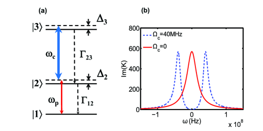
Figure 1: (Color online) (a) Energy-level diagram and excitation scheme of the three-level ladder-type atoms, in which the states $|2\rangle$ and $|1\rangle$ are coupled by the probe field with angular frequency $\omega_{p}$, and the states $|3\rangle$ and $|2\rangle$ are coupled by the control field with angular frequency $\omega_{c}$. $\Delta_{2}$ and $\Delta_{3}$ are respectively one- and two-photon detunings; $\Gamma_{13}$ ($\Gamma_{23}$) is the spontaneous emission decay rate from $|3\rangle$ to $|1\rangle$ ($|3\rangle$ to $|2\rangle$). (b) The absorption spectrum Im($K$) of the probe field as a function of $\omega$. The solid and dashed lines correspond respectively to $\Omega_{c}$ =0 (no EIT) and $\Omega_{c}$=40 MHz (EIT).

For simplicity, we assume both the probe and the control fields propagate along the $z$ direction. Then the electric field of the system can be expressed as $\mathbf{E}$=$\sum_{l=p,c}\mathbf{e}_{l}{\cal E}_{l}{\rm exp}[i(k_{l}z-\omega_{l}t)]+{\rm c.c.}$. Here $\mathbf{e}_{p}$ and $\mathbf{e}_{c}$ (${\cal E}_{p}$ and ${\cal E}_{c}$) are respectively the polarization unit vectors (envelopes) of the probe and control field; $k_{p}=\omega_{p}/c$ and $k_{c}=\omega_{c}/c$ are respectively the wavenumbers of the probe and control fields before entering the medium.

Under electric-dipole and rotating-wave approximations, the equations of the motion for the density matrix elements in interaction picture read julio

$$\frac{\partial}{\partial t}\sigma_{11}=i\Omega_{p}^{*}\sigma_{21}-i\Omega_{p}\sigma_{21}^{*}+\Gamma_{12}\sigma_{22},$$ (1a)

$$\frac{\partial}{\partial t}\sigma_{22}=i\Omega_{p}\sigma_{21}^{*}+i\Omega_{c}^{*}\sigma_{32}-i\Omega_{p}^{*}\sigma_{21}-i\Omega_{c}\sigma_{32}^{*}-\Gamma_{12}\sigma_{22}+\Gamma_{23}\sigma_{33},$$ (1b)

$$\frac{\partial}{\partial t}\sigma_{33}=i\Omega_{c}\sigma_{32}^{*}-i\Omega_{c}^{*}\sigma_{32}-\Gamma_{3}\sigma_{33},$$ (1c)

$$\frac{\partial}{\partial t}\sigma_{21}=id_{21}\sigma_{21}+i\Omega_{p}(\sigma_{11}-\sigma_{22})+i\Omega_{c}^{*}\sigma_{31},$$ (1d)

$$\frac{\partial}{\partial t}\sigma_{31}=id_{31}\sigma_{31}-i\Omega_{p}\sigma_{32}+i\Omega_{c}\sigma_{21},$$ (1e)

$$\frac{\partial}{\partial t}\sigma_{32}=id_{32}\sigma_{32}+i\Omega_{c}(\sigma_{22}-\sigma_{33})-i\Omega_{p}^{*}\sigma_{31},$$ (1f)

where $\Omega_{p}=(\mathbf{e}_{p}\cdot\mathbf{p}_{21}){\cal E}_{p}/\hbar$ and $\Omega_{c}=(\mathbf{e}_{c}\cdot\mathbf{p}_{32}){\cal E}_{c}/\hbar$ are respectively the half Rabi frequencies of the probe and the control fields, with $\mathbf{p}_{ij}$ the electric dipole matrix element associated with the transition between $|j\rangle$ and $|i\rangle$. In Eq. (1), $d_{21}=\Delta_{2}+i\gamma_{21}$, $d_{31}=\Delta_{3}+i\gamma_{31}$, and $d_{32}=(\Delta_{3}-\Delta_{2})+i\gamma_{32}$, with $\Delta_{2}=\omega_{p}-(\omega_{2}-\omega_{1})$ and $\Delta_{3}=\omega_{p}+\omega_{c}-(\omega_{3}-\omega_{1})$ respectively the one-photon and two-photon detunings; $\gamma_{ij}=(\Gamma_{i}+\Gamma_{j})/2+\gamma_{ij}^{\rm col}$, $\Gamma_{j}=\sum_{i<j}\Gamma_{ij}$, with $\Gamma_{ij}$ denoting the spontaneous emission decay rate from $|j\rangle$ to $|i\rangle$ and $\gamma_{ij}^{\rm col}$ denoting the dephasing rate between the states $|i\rangle$ and $|j\rangle$ Boyd .

The evolution of the electric field is governed by the Maxwell equation, which under a slowly varying envelope approximation yields li08

$$i\left(\frac{\partial}{\partial z}+\frac{1}{c}\frac{\partial}{\partial t}\right)\Omega_{p}+\kappa_{12}\sigma_{21}=0,$$ (2a)

$$i\left(\frac{\partial}{\partial z}+\frac{1}{c}\frac{\partial}{\partial t}\right)\Omega_{c}+\kappa_{23}\sigma_{32}=0,$$ (2b)

where $\kappa_{12}={\cal N}_{a}\omega_{p}|\mathbf{p}_{12}|^{2}/(2\varepsilon_{0}\rm c\hbar)$ and $\kappa_{23}={\cal N}_{a}\omega_{c}|\mathbf{p}_{23}|^{2}/(2\varepsilon_{0}\rm c\hbar)$, with ${\cal{N}}_{a}$ the atomic density. Note that for simplicity we have assumed both the probe and control fields have large beam radius in both $x$ and $y$ directions so that the diffraction effect representing by the term $(\partial^{2}/\partial x^{2}+\partial^{2}/\partial y^{2})\Omega_{p,c}$ can be neglected.

III Ultraslow optical solitons

III.1 Nonlinear envelope equation

We first consider the formation and propagation of ultraslow optical solitons in the system. We assume the probe field is weakly nonlinear and pulsed with time duration $\tau_{0}$; the control field is a continuous-wave (i.e. its time duration is much larger than $\tau_{0}$) and strong enough so that its depletion can be neglected during propagation, which means $\Omega_{c}$ can be taken as a constant and hence Eq. (2b) can be disregarded.

In order to derive the nonlinear envelope equation of the probe field, we make the asymptotic expansion $\sigma_{jl}=\sigma_{jl}^{(0)}+\epsilon\sigma_{jl}^{(1)}+\epsilon^{2}\sigma_{jl}^{(2)}+\epsilon^{3}\sigma_{jl}^{(3)}+\cdots$, $\Omega_{p}=\epsilon\Omega_{p}^{(1)}+\epsilon^{2}\Omega_{p}^{(2)}+\epsilon^{3}\Omega_{p}^{(3)}+\cdots$, with $\sigma_{jl}^{(0)}=\delta_{j1}\delta_{l1}$ and $\epsilon$ a small parameter characterizing the amplitude of $\Omega_{p}$. To obtain a divergence-free expansion, all quantities on the right hand side of the expansion are considered as functions of the multiscale variables $z_{l}=\epsilon^{l}z$ $(l=0,1,2)$, and $t_{l}=\epsilon^{l}t$ $(l=0,1)$.

Substituting the above expansion to the MB Eqs. (1) and (2a) and comparing the the coefficients of $\epsilon^{l}$ $(l=1,2,3...)$, we obtain a set of linear but inhomogeneous equations which can be solved order by order. At the first order, we obtain the solution

$$\Omega_{p}^{(1)}=F\,e^{i\theta},$$ (3a)

$$\sigma_{21}^{(1)}=\frac{\omega+d_{31}}{D(\omega)}Fe^{i\theta},$$ (3b)

$$\sigma_{31}^{(1)}=-\frac{\Omega_{c}}{D(\omega)}Fe^{i\theta},$$ (3c)

with other $\sigma_{jl}^{(1)}$=0. In the above expressions, $D(\omega)=|\Omega_{c}|^{2}-(\omega+d_{21})(\omega+d_{31})$, $\theta=K(\omega)z_{0}-\omega t_{0}$ note0 with $F$ the envelope function of the slow variables $z_{l}$, $z_{2}$, and $t_{1}$; $K(\omega)$ is the linear dispersion relation of the system, given by

$$K(\omega)=\frac{\omega}{c}+\frac{\kappa_{12}(\omega+d_{31})}{D(\omega)}.$$ (4)

Fig. 1(b) shows Im($K$), i.e. the imaginary part of $K$, as a function of $\omega$. When plotting the figure, we have chosen ultracold Rydberg atoms with the levels in Fig. 1(a) and the system parameters as Maxwell2013 ; adams2010 :

$$|1\rangle=|5s^{2}S_{1/2},F=2\rangle,\,\,\,\,|2\rangle=|5p^{2}P_{3/2},F=3\rangle,\,\,\,\,|3\rangle=|60s^{2}S_{1/2},\rangle.$$ (5)

$$\Gamma_{12}/2\pi=6\,\,{\rm MHz},\,\,\,\,\Gamma_{23}/2\pi=3200\,\,{\rm Hz},\,\,\,\,\gamma_{21}\approx 18.8\,\,{\rm MHz},\,\,\,\,\gamma_{31}\approx 1000\,\,{\rm Hz}.$$ (6)

In addition, we assume ${\cal N}_{a}\approx 1.79\times 10^{11}$ $\rm cm^{-3}$, then $\kappa_{12}$ takes the value $1.0\times 10^{10}$ ${\rm cm}^{-1}{\rm s}^{-1}$. The solid and dashed line in Fig. 1(b) correspond, respectively, to the absence ($\Omega_{c}=0$) and the presence ($\Omega_{c}=40$ ${\rm MHz}$) of the control field. We see that in the absence of $\Omega_{c}$ the probe field has a large absorption (the solid line in Fig. 1(b) ) (i.e. no EIT); however, in the presence of $\Omega_{c}$ a transparency window is opened in Im($K$) (the dashed line in Fig. 1(b) ), and hence the probe pulse can propagate in the resonant atomic system with negligible absorption (i.e. EIT). The openness of the EIT transparency window is due to the quantum interference effect induced by the control field.

At the second order, a divergence-free condition requires

$$\frac{\partial F}{\partial z_{1}}+\frac{1}{V_{g}}\frac{\partial F}{\partial t_{1}}=0,$$ (7)

with $V_{g}=(\partial K/\partial\omega)^{-1}$ being the group velocity of $F$. The second-order solution reads $\sigma_{21}^{(2)}=A_{21}^{(2)}(\partial F/\partial t_{1})e^{i\theta}$, $\sigma_{31}^{(2)}=A_{31}^{(2)}(\partial F/\partial t_{1})e^{i\theta}$, $\sigma_{11}^{(2)}=A_{11}^{(2)}|F|^{2}e^{-2\bar{\alpha}z_{2}}$, $\sigma_{33}^{(2)}=A_{33}^{(2)}|F|^{2}e^{-2\bar{\alpha}z_{2}}$, $\sigma_{32}^{(2)}=A_{32}^{(2)}|F|^{2}e^{-2\bar{\alpha}z_{2}}$ with

$$A_{21}^{(2)}=\frac{i}{\kappa_{12}}\left(\frac{1}{V_{{\rm g}}}-\frac{1}{c}\right),$$ (8a)

$$A_{31}^{(2)}=\frac{i}{\Omega_{c}^{\ast}}\left[-\frac{\omega+d_{31}}{D(\omega)}-\frac{\left(\omega+d_{21}\right)}{\kappa_{12}}\left(\frac{1}{V_{{\rm g}}}-\frac{1}{c}\right)\right],$$ (8b)

$$A_{11}^{(2)}=\frac{[i\Gamma_{23}-2|\Omega_{c}|^{2}M]N-i\Gamma_{12}\left(\frac{|\Omega_{c}|^{2}}{D(\omega)^{\ast}d_{32}^{\ast}}-\frac{|\Omega_{c}|^{2}}{D(\omega)d_{32}}\right)}{-\Gamma_{12}\Gamma_{23}-i\Gamma_{12}|\Omega_{c}|^{2}M},$$ (8c)

$$A_{33}^{(2)}=\frac{1}{i\Gamma_{12}}\left(N-i\Gamma_{12}A_{11}^{(2)}\right)|F|^{2}e^{-2\bar{\alpha}z_{2}},$$ (8d)

$$A_{32}^{(2)}=\frac{1}{d_{32}}\left(-\frac{\Omega_{c}}{D(\omega)}+2\Omega_{c}A_{33}^{(2)}+\Omega_{c}A_{11}^{(2)}\right),$$ (8e)

where $\bar{\alpha}=\epsilon^{-2}\alpha=\epsilon^{-2}$Im$[K(\omega)]$, $M=1/d_{32}-1/d_{32}^{\ast}$, and $N=(\omega+d_{31}^{\ast})/D(\omega)^{\ast}-(\omega+d_{31})/D(\omega)$.

With the above result we proceed to third order. The divergence-free condition in this order yields the nonlinear equation for $F$:

$$i\frac{\partial F}{\partial z_{2}}-\frac{1}{2}K_{2}\frac{\partial^{2}F}{\partial t_{1}^{2}}-We^{-2\bar{\alpha}z_{2}}|F|^{2}F=0,$$ (9)

where $K_{2}\equiv\partial^{2}K/\partial\omega^{2}$ and $W=-\kappa_{12}\left[\Omega_{c}^{\ast}A_{32}^{(2)}+(\omega+d_{31})(2a_{11}^{(2)}+A_{33}^{(2)})\right]/D(\omega)$ are dispersion and nonlinear (Kerr) coefficients, respectively.

III.2 Ultraslow optical solitons

Combining Eqs. (7) and (9) and returning to the original variables we obtain

$$i\left(\frac{\partial}{\partial z}+\alpha\right)U-\frac{K_{2}}{2}\frac{\partial^{2}U}{\partial\tau^{2}}-W|U|^{2}U=0,$$ (10)

where $\tau=t-z/V_{g}$ and $U=\epsilon Fe^{-\bar{\alpha}z_{2}}$. Due to the resonant character of the system, the NLS equation (10) has complex coefficients. Generally, such equation does not allow soliton solution. However, if the imaginary part of the coefficients can be made much smaller than their real part, it is possible to form solitons in the system. We shall show below this can indeed be achieved in the present EIT system.

For the ultracold Rydberg atoms with the energy-levels assigned by (5) and the system parameters given by (6), we obtain $K_{0}=(0.23+i0.0002)$ ${\rm cm^{-1}}$, $K_{1}=(1.15+i0.0009)\times 10^{-7}$ ${\rm cm^{-1}s}$, $K_{2}=(1.82+i0.05)\times 10^{-15}$ ${\rm cm^{-1}s^{2}}$, $W=(2.59+i0.002)\times 10^{-18}$ ${\rm cm^{-1}s^{2}}$ when selecting $\Delta_{2}=700$ ${\rm MHz}$, $\Delta_{3}=2$ ${\rm MHz}$, $\kappa_{12}=1\times 10^{10}$ ${\rm cm^{-1}}{\rm s^{-1}}$, and $\Omega_{c}=300$ ${\rm MHz}$. We see that the imaginary parts of the coefficients of the NLS equation (10) are indeed much smaller than their corresponding real parts. As a result, Eq. (10) can be approximated as the following dimensionless form

$$i\frac{\partial u}{\partial s}+\frac{\partial^{2}u}{\partial\sigma^{2}}+2u|u|^{2}=i\nu u,$$ (11)

with $s=-z/(2L_{D})$, $\sigma=\tau/\tau_{0}$, and $u=U/U_{0}$, and $\nu=2L_{D}/L_{A}$. Here $L_{D}\equiv{\tau_{0}}^{2}/|\tilde{K}_{2}|$, $L_{A}\equiv 1/(2\alpha)$, and $U_{0}\equiv(1/\tau_{0})\sqrt{|\tilde{K}_{2}/\tilde{W}|}$ are characteristic dispersion length, absorption length, and Rabi frequency of the probe field, respectively. Note that in order to obtain soliton solutions we have assumed $L_{D}$ is equal to $L_{\rm NL}\equiv 1/(U_{0}^{2}\tilde{W})$ (the characteristic nonlinearity length). The tilde symbol means taking real part (e.g. $\tilde{K}_{2}={\rm Re}(K_{2})$).

If taking $\tau_{0}=1.0\times 10^{-7}$ ${\rm s}$, we obtain $U_{0}=2.65\times 10^{8}$ ${\rm s^{-1}}$, $L_{D}=$ $L_{\rm NL}=5.48$ $\rm cm$, $L_{A}=2500$ $\rm cm$. Because $L_{A}$ is much larger than $L_{D}$ and $L_{\rm NL}$ which gives $\nu=0.0044$, the absorption term on the right hand side of Eq. (11) can be neglected in the leading-order approximation. Thus we obtain a standard NLS equation that is completely integrable and allows various soliton solutions. After returning to the original variables, the half Rabi frequency of the probe field corresponding to single-soliton solution reads

$$\Omega_{p}(z,t)=\frac{1}{\tau_{0}}\sqrt{\frac{\tilde{K_{2}}}{\tilde{W}}}{\rm sech}\left[\frac{1}{\tau_{0}}\left(t-\frac{z}{\tilde{V_{g}}}\right)\right]{\rm exp}{\left[i\tilde{K}_{0}z-i\frac{z}{2L_{D}}\right]},$$ (12)

where $\tilde{K}_{0}=\tilde{K}(\omega)\mid_{\omega=0}$. With the above system parameters, we obtain

$$\tilde{V}_{g}=3\times 10^{-4}\,c,$$ (13)

i.e. the soliton has an ultraslow propagating velocity, which is essential for its storage and retrieval considered in the next section.

Shown in Fig. 2(a)

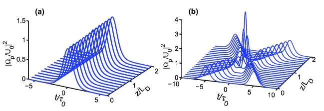
Figure 2: (Color online) Propagation of the ultraslow optical soliton and the interaction between two solitons. (a) Waveshape $|\Omega_{p}/U_{0}|^{2}$ of the ultraslow optical soliton as a function of $z/L_{D}$ and $t/\tau_{0}$. (b) Collision between two ultraslow optical solitons.

is the numerical result of the waveshape $|\Omega_{p}/U_{0}|^{2}$ of the ultraslow optical soliton as a function of $z/L_{D}$ and $t/\tau_{0}$. When making the calculation, Eq. (11) is used with the solution (12) as an initial condition. Fig. 2(b) shows the collision between two ultraslow optical solitons, with the initial condition given by $u(0,\sigma)={\rm sech}(\sigma-5)\exp(-i\sigma)+{\rm sech}(\sigma+5)\exp(i\sigma)$. We see that the ultraslow optical solitons are robust during the propagation and the collision.

It is easy to calculate the threshold of the optical power density $P_{\rm max}$ for generating the ultracold optical soliton predicted above by using Poynting’s vector huang2005 . We obtain

$$P_{\rm max}=9.38\times 10^{-5}\,\,{\rm W}.$$ (14)

Thus, to generate the ultraslow optical solitons in the system, very low input power is needed.

IV Storage and retrieval of the ultraslow optical solitons

In a pioneered work Fleischhauer2000 , Fleischhauer and Lukin showed the possibility of storage and retrieval of optical pulses in a three-level atomic system with a $\Lambda$-type level configuration. They demonstrated that, when switching on control field, probe pulse propagates in the atomic medium with nearly vanishing absorption; by slowly switching off the control field the probe pulse disappears and gets stored in the form of atomic coherence; when the control field is switched on again the probe pulse reappears. However, the intensity of the probe pulse used in Ref. Fleischhauer2000 and a series of studies carried out later on (see Refs. LDBH ; phillip2001 ; Longd ; schnorr2009 ; Zhao ; zhang2009 ; Rad ; Dudin10 ; Yangf ; PFMWL ; dudin2013 ; Dai ; heinze2013 and references therein) is weak, i.e. systems used in those studies Fleischhauer2000 ; LDBH ; phillip2001 ; Longd ; schnorr2009 ; Zhao ; zhang2009 ; Rad ; Dudin10 ; Yangf ; PFMWL ; dudin2013 ; Dai ; heinze2013 work in linear regime. Now, we extend these studies into a weakly nonlinear regime, and demonstrate that it is possible to realize the storage and retrieval of ultraslow optical solitons in the ladder-type atomic system via EIT.

To this end, we consider the solution of the MB equations presented in Sec. II. We stress that for the storage and retrieval of optical solitons the dynamics of the control-field must be taken into account, i.e. Eq. (2b) must be solved together with Eqs. (1) and (2a). Because in this case analytical solutions are not available, we resort to numerical simulation.

Fig. 3 shows

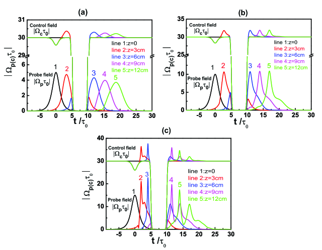
Figure 3: (Color online) Time evolution of $|\Omega_{p}\tau_{0}|$ and $|\Omega_{c}\tau_{0}|$ as functions of $z$ and $t$ for different input light intensities. (a) Storage and retrieval of weak (i.e. linear) pulse, with $\Omega_{p}(0,t)\tau_{0}=5\,{\rm sech}(t/\tau_{0})$. (b) Storage and retrieval of soliton pulse, with $\Omega_{p}(0,t)\tau_{0}=10\,{\rm sech}(t/\tau_{0})$. (c) Storage and retrieval of strong pulse, with $\Omega_{p}(0,t)\tau_{0}=15\,{\rm sech}(t/\tau_{0})$. The lines from 1 to 5 in each panel correspond to $z$=0, 3 cm, 6 cm, 9 cm, and 12 cm, respectively.

the time evolution of $|\Omega_{p}\tau_{0}|$ and $|\Omega_{c}\tau_{0}|$ as functions of $z$ and $t$ for different input light intensities. In the simulation, the switching-on and the switching-off the control field is modeled by the combination of two hyperbolic tangent functions with the form

$$\Omega_{c}(0,t)=\Omega_{c0}\left\{1-\frac{1}{2}{\rm tanh}\left[\frac{t-T_{\rm off}}{T_{s}}\right]+\frac{1}{2}{\rm tanh}\left[\frac{t-T_{\rm on}}{T_{s}}\right]\right\},$$ (15)

where $T_{\rm off}$ and $T_{\rm on}$ are respectively the times of switching-off and the switching-on of the control field with a switching time approximately given by $T_{s}$. The system parameters are chosen from a typical cold alkali ⁸⁷Rb atomic gas with $\Gamma_{12}/2\pi=6$ ${\rm MHz}$, $\Gamma_{23}/2\pi=3.2$ ${\rm KHz}$, $\gamma_{21}\tau_{0}\approx 1.88$, $\gamma_{31}\tau_{0}\approx 10^{-4}$, $\Delta_{2}\tau_{0}=70$, $\Delta_{3}\tau_{0}=0.2$, $\kappa_{12}\tau_{0}=1\times 10^{3}$ ${\rm cm^{-1}}$, $\kappa_{23}\tau_{0}=2\times 10^{3}$ ${\rm cm^{-1}}$, $\Omega_{c0}\tau_{0}=30$, $\rm T_{s}/\tau_{0}=0.2$, $T_{\rm off}/\tau_{0}=5$, $T_{\rm on}/\tau_{0}=10$, with $\tau_{0}=10^{-7}{\rm s}$. The waveshape of the input probe pulse is taken as a hyperbolic secant one, i.e., $\Omega_{p}(0,t)=\Omega_{p0}\,{\rm sech}(t/\tau_{0})$, with different $\Omega_{p0}$ to represent weak (i.e. linear), soliton (i.e. weak nonlinear), and strong probe regimes. Lines from 1 to 5 are for $z=0$, 3 cm, 6 cm, 9 cm, and 12 cm, respectively.

Shown in Fig. 3(a) is the result for a weak (i.e. linear) probe pulse, where $\Omega_{p}(0,t)\tau_{0}=5\,{\rm sech}(t/\tau_{0})$. In this case, the system is dispersion-dominant. Storage and retrieval of light pulses are possible, but the probe pulse broadens fast before and after the storage, which is not desirable for practical applications because light information will be lost after the storage.

Fig. 3(b) shows the result for a weak nonlinear (i.e. soliton) probe pulse, where $\Omega_{p}(0,t)\tau_{0}=10\,{\rm sech}(t/\tau_{0})$. In this situation, the system works in the regime with a balance between dispersion and nonlinearity. We see that the probe pulse evolves firstly into a soliton (i.e. its pulse width is narrowed) before the storage; later on the soliton is stored in the atomic medium (i.e. $\Omega_{p}=0$ when $\Omega_{c}$ is switched off); then the soliton is retrieved after the storage (when $\Omega_{c}$ is switched on). The retrieved soliton has nearly the same waveshape as that before the storage.

Shown in Fig. 3(c) is the result for a strong probe pulse, where $\Omega_{p}(0,t)\tau_{0}=15\,{\rm sech}(t/\tau_{0})$. In this case, the system works in a strong nonlinear (i.e. nonlinearity-dominant) regime and hence a stable soliton is not possible. From the figure we see that the probe pulse has a significant distortion, especially some new peaks are generated. Due to the large distortion, the light information will be lost fast even before the storage.

From the result of Fig. 3, we conclude that, comparing with the linear pulse and the strong nonlinear pulse, the soliton pulse is desirable for the storage and retrieval. One may ask the question how the optical soliton is stored into the atoms when both the probe and control fields have vanishing value. In fact, during the light storage the probe-field energy is converted into atomic degrees of freedom, i.e. the atomic coherence $\sigma_{13}$ has non-vanishing value even when both $\Omega_{c}$ and $\Omega_{p}$ are zero.

Shown in Fig. 4

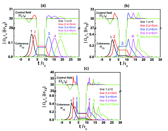
Figure 4: (Color online) The atomic coherence $\sigma_{13}$ as functions of distance $z$ and time $t$ for different input light intensities. Corresponding evolution of $|\Omega_{c}\tau_{0}|$ is also shown. Initial probe pulses used in panels (a),(b), and (c) are the same as those used in Fig. 3(a), Fig. 3(b), and Fig. 3(c), respectively. The lines from 1 to 5 in each panel correspond to $z$=0, 3 cm, 6 cm, 9 cm, and 12 cm, respectively.

is the result of $\sigma_{13}$ for different input light intensities as functions of $z$ and $t$. Corresponding evolution of $|\Omega_{c}\tau_{0}|$ is also plotted. Initial probe pulses used in each panels of the figure are the same as those used in Fig. 3. The lines from 1 to 5 in each panel of the figure correspond to $z$=0, 3 cm, 6 cm, 9 cm, and 12 cm, respectively. From Fig. 4 combining with Fig. 3 we see that indeed $\sigma_{13}\neq 0$ in the time interval when $\Omega_{c}=\Omega_{p}=0$. Since the probe pulse is stored in the form of atomic coherence $\sigma_{13}$ when the control field is switched off and is retained until the control field is switched on again, the atomic coherence $\sigma_{13}$ can be taken as the intermediary for the storage and retrieval of the probe pulse.

Now we give a simple explanation on the numerical result given above. Note that when the control pulse is switching off, the probe pulse becomes nearly zero. Thus in the weak nonlinear regime, the probe pulse can be approximated as

$$\Omega_{p}(z,t)\approx\left\{\begin{array}[]{lll}\frac{A}{\tau_{0}}\sqrt{\frac{\tilde{K}_{2}}{\tilde{W}}}{\rm sech}\left[\frac{1}{\tau_{0}}\left(t-\frac{z}{\tilde{V_{g}}}\right)\right]e^{i[\tilde{K}_{0}-1/(2L_{D})]z},\,\,{\rm for}\,\,t<{\rm T_{off}},\\ 0,\,\,\,\,{\rm for}\,\,{\rm T_{off}}\leq t\leq{\rm T_{on}},\\ \frac{B}{\tau_{0}}\sqrt{\frac{\tilde{K}_{2}}{\tilde{W}}}{\rm sech}\left[\frac{1}{\tau_{0}}\left(t-\frac{z}{\tilde{V_{g}}}\right)\right]e^{i[\tilde{K}_{0}-1/(2L_{D})]z+i\phi_{0}},\,\,{\rm for}\,\,t>{\rm T_{on}},\end{array}\right.$$ (16)

where $A$ and $B$ are constants depending on initial condition, $\phi_{0}$ is a constant phase factor.

From both Fig. 3 and Fig. 4, we see that the control field is changed before and after the storage of the probe field. To analyze the dynamics (depletion) of the control field before and after the storage of the probe soliton, we solve Eq. (2b) using a perturbation method. The numerical result shown in Fig. 3 and Fig. 4 suggests us to make the perturbation expansion

$$\Omega_{c}=\Omega_{c}^{(0)}+\epsilon\Omega_{c}^{(1)}+\epsilon^{2}\Omega_{c}^{(2)},$$ (17)

which is valid for the time interval before and after the probe soliton storage where the leading-order of $\Omega_{c}$ (i.e. $\Omega_{c}^{(0)}$) has a large value. Substituting the expansion (17) into Eq. (2b) and solving the equations for $\Omega_{c}^{(l)}$ ($l=0,1,2$), we obtain the following conclusions: (i) $\Omega_{c}^{(0)}$ is a constant, which corresponds to the horizontal line in the upper part of Fig. 3 and Fig. 4. (ii) $\Omega_{c}^{(1)}(t,z)=\Omega_{c}^{(1)}(t-z/c)$ describes a hole below the horizontal line in the upper part of Fig. 3 and Fig. 4, which propagates with velocity $c$ (i.e. the light speed in vacuum). The concrete form of $\Omega_{c}^{(1)}$ relies on initial condition. (iii) $\Omega_{c}^{(2)}$ satisfies the equation $i\partial\Omega_{c}^{(2)}/\partial z=-\kappa_{23}\sigma_{32}^{(2)}$. Thus we obtain

$$\Omega_{c}^{(2)}=i\frac{\kappa_{23}\Delta_{3}}{(|\Omega_{c}|^{2}-\Delta_{2}\Delta_{3})^{2}}\frac{1}{\tau_{0}^{2}}\frac{\tilde{K}_{2}}{\tilde{W}}\tanh\left[\frac{1}{\tau_{0}}\left(t-\frac{z}{\tilde{V}_{g}}\right)\right],$$ (18)

which has propagating velocity $\tilde{V_{g}}$ and contributes a small hump to the horizontal line in the upper part of Fig. 3 and Fig. 4. That is to say, the hump propagates with the same velocity as the probe soliton. Physically, the appearance of the control field hump (depletion) is due to the energy exchange between the control field and the probe field via the atomic system as an intermediary.

In addition, we can also provide a simple theoretical explanation on the behavior observed in Fig. 4(b), where, before and after the storage of the probe soliton, $\sigma_{13}$ behaves like a soliton but it is constant during the storage. First, let us consider the time interval before and after the storage of the probe soliton where $\Omega_{c}\approx\Omega_{c}^{(0)}$ (for simplicity we neglect the small hump described by Eq. (18)). In this region, the perturbation expansion given in Sec. IIIA is still valid. Thus the result obtained there can be used here. From Eqs. (3a) and (3c), when evaluated at the center frequency of the probe pulse (i.e. $\omega=0$) we obtain

$$\sigma_{13}=-\frac{\Omega_{c}^{*}}{D^{*}(0)}\Omega_{p}^{*}\approx-\frac{\Omega_{c}^{*(0)}}{D^{*}(0)}\frac{1}{\tau_{0}}\sqrt{\frac{\tilde{K_{2}}}{\tilde{W}}}{\rm sech}\left[\frac{1}{\tau_{0}}\left(t-\frac{z}{\tilde{V_{g}}}\right)\right]{\rm exp}{\left[-i\tilde{K}_{0}z+i\frac{z}{2L_{D}}\right]}.$$ (19)

We see that, before and after the storage of the probe soliton, $\sigma_{13}$ is also soliton with the propagating velocity $\tilde{V_{g}}$, as expected.

The behavior of $\sigma_{13}$ in the time interval during the probe-soliton storage can not be explained by using the perturbation theory developed in Sec. IIIA because in this case $\Omega_{c}$ is a small quantity. To solve this problem, we start to consider the Bloch Eq. (1) directly milo . Since $d_{31}\sigma_{31}$ and $\Omega_{p}\sigma_{32}$ are small, by Eq. (1e) we have

$$\sigma_{21}\approx-\frac{i}{\Omega_{c}}\frac{\partial\sigma_{31}}{\partial t}.$$ (20)

Furthermore, since $\sigma_{11}\approx 1$ and $\sigma_{22}\approx 0$, Eq. (1d) gives

$$\sigma_{31}\approx-\frac{\Omega_{p}}{\Omega_{c}^{*}}+\frac{1}{i\Omega_{c}^{*}}\left(\frac{\partial}{\partial t}-id_{21}\right)\sigma_{21}.$$ (21)

Substituting Eq. (20) into Eq. (21) we obtain

$$\sigma_{13} =-\frac{\Omega_{p}^{*}}{\Omega_{c}}-\frac{1}{|\Omega_{c}|^{2}}\left(\frac{\partial}{\partial t}+id_{21}\right)\sigma_{13}$$ (22)

$$\approx-\frac{\Omega_{p}^{*}}{\Omega_{c}}.$$

Although in the time interval of the storage both the probe and control fields tend into zero, the ratio $\Omega_{p}^{*}/\Omega_{c}$ can keep a finite constant value, as shown in the numerical simulation presented in Fig. 4. The physical reason is that in our study the system starts from the dark state $|D\rangle=\Omega_{c}^{*}|1\rangle-\Omega_{p}|3\rangle=\Omega_{c}^{*}(|1\rangle-(\Omega_{p}^{*}/\Omega_{c})^{*}|3\rangle)$ and it approximately keeps in this dark state during time evolution. As a result, the atomic coherence $\sigma_{13}$ can have a nonzero value even both $\Omega_{c}$ and $\Omega_{p}$ are small.

V SUMMARY

In the present contribution, we have proposed a method for obtaining stable nonlinear optical pulses and realizing their storage and retrieval in an ultracold ladder-type three-level atomic gas via EIT. Starting from the MB equations, we have derived a NLS equation governing the evolution of probe-field envelope. We have shown that optical solitons with ultraslow propagating velocity and extremely low generation power can be created in the system. Furthermore, we have demonstrated that such ultraslowly propagating, ultralow-light level optical solitons can be stored and retrieved by switching off and on the control field. Because of the balance between dispersion and nonlinearity, the ultraslow optical solitons are robust during propagation, and hence their storage and retrieval are more desirable than that of linear optical pulses. Our study provides a possibility of realizing light information storage and retrieval by using solitonlike nonlinear optical pulses.

- (1) M. Fleischhauer, A. Imamoglu, and J. P. Marangos, Rev. Mod. Phys. 77, 633 (2005).
- (2) M. Fleischhauer and M. D. Lukin, Phys. Rev. Lett. 84, 5094 (2000).
- (3) C. Liu, Z. Dutton, C. Behroozi, and L. Hau, Nature 409, 490 (2001).
- (4) D. F. Phillips, A. Fleischhauer, A. Mair, R. L. Walsworth, and M. D. Lukin, Phys. Rev. Lett. 86, 783 (2001).
- (5) J. J. Longdell, E. Fraval, M. J. Sellars, and N. B. Manson, Phys. Rev. Lett. 95, 063601 (2005).
- (6) U. Schnorrberger, J. D. Thompson, S. Trotzky, R. Pugatch, N. Davidson, S. Kuhr, and I. Bloch, Phys. Rev. Lett. 103, 033003 (2009).
- (7) R. Zhao, Y. O. Dudin, S. D. Jenkins, C. J. Campbel, D. N. Matsukevich, T. A. B. Kennedy, and A. Kuzmich, Nat. Phys. 5, 95 (2009).
- (8) R. Zhang, S. R. Garner, and L. V. Hau, Phys. Rev. Lett. 103, 233603 (2009).
- (9) A. G. Radnaev, Y. O. Dudin, R. Zhao, H. H. Jen, S. D. Jenkins, A. Kuzmich, and T. A. B. Kennedy, Nat. Phys. 6, 894 (2010).
- (10) Y. O. Dudin, R. Zhao, T. A. B. Kennedy, and A. Kuzmich, Phys. Rev. A 81, 041805(R) (2010).
- (11) F. Yang, T. Mandel, C. Lutz, Z.-S. Yuan, and J.-W. Pan, Phys. Rev. A 83, 063420 (2011).
- (12) I. Novikova, R. L. Walsworth, and Y. Xiao, Laser Photonics Rev. 6, 333 (2012).
- (13) H.-N. Dai, H. Zhang, S.-J. Yang, T.-M. Zhao, J. Rui, Y.-J. Deng, L. Li, N.-L. Liu, S. Chen, X.-H. Bao, X.-M. Jin, B. Zhao, and J.-W. Pan, Phys. Rev. Lett. 108, 210501 (2012).
- (14) Y. O. Dudin, L. Li, and A. Kuzmich, Phys. Rev. A 87, 031801 (2013).
- (15) G. Heinze, C. Hubrich, and T. Halfmann, Phys. Rev. Lett 111, 033601 (2013).
- (16) T. N. Dey and G. S. Agarwal, Phys. Rev. A 67, 033813 (2003).
- (17) M. Saffman, T. G. Walker, K. Molmer, Rev. Mod. Phys. 82, 2314 (2010).
- (18) J. D. Pritchard, K. J. Weatherill, and C. S. Adams, Annu. Rev. Cold At. Mol. 1, 301 (2013).
- (19) Y. Wu and L. Deng, Opt. Lett. 29, 2064 (2004).
- (20) G. Huang, L. Deng, and M. G. Payne, Phys. Rev. E 72, 016617 (2005).
- (21) D. Maxwell, D. J. Szwer, D. Paredes-Barato, H. Busche, J. D. Pritchard, A. Gauguet, K. J. Weatherill, M. P. A. Jones, and C. S. Adams, Phys. Rev. Lett. 110, 103001 (2013).
- (22) M. Saffman, T. G. Walker, and K. Molmer, Rev. Mod. Phys. 82, 2313 (2010).
- (23) J. D. Pritchard, K. J. Weatherill, and C. S. Adams, Annu. Rev. Cold At. Mol. 1, 301 (2013).
- (24) J. Gea-Banacloche, Y.-q. Li, S.-z. Jin, and M. Xiao, Phys. Rev. A 51, 576 (1995).
- (25) R. W. Boyd, Nonlinear Optics (3rd edition) (Academic, Elsevier, 2008).
- (26) H.-j. Li and G. Huang, Phys. Lett. A 372, 4127 (2008).
- (27) The frequency and wave number of the probe field are given by and respectively. Thus corresponds to the center frequency of the probe field.
- (28) J. D. Pritchard, D. Maxwell, A. Gauguet, K. J. Weatherill, M. P. A. Jones, and C. S. Adams, Phys. Rev. Lett 105, 193603 (2010).
- (29) P. W. Milonni, Fast Light, Slow Light and Left-Handed Light (Institute of Physics Publishing, Bristol and Philadelphia, 2005), Sec. 6.2.