11email: sandree@ph1.uni-koeln.de
Modelling clumpy PDRs in 3D
Abstract
Context. Models of photon-dominated regions (PDRs) still fail to fully reproduce some of the observed properties, in particular the combination of the intensities of different PDR cooling lines together with the chemical stratification, as observed e.g. for the Orion Bar PDR.
Aims. We aim to construct a numerical PDR model, KOSMA- 3D, to simulate full spectral cubes of line emission from arbitrary PDRs in three dimensions (3D). The model is to reproduce the intensity of the main cooling lines from the Orion Bar PDR and the observed layered structure of the different transitions.
Methods. We build up a 3D compound, made of voxels (“3D pixels”) that contain a discrete mass distribution of spherical “clumpy” structures, approximating the fractal ISM. To analyse each individual clump the new code is combined with the KOSMA- PDR model. Probabilistic algorithms are used to calculate the local FUV flux for each voxel as well as the voxel-averaged line emissivities and optical depths, based on the properties of the individual clumps. Finally, the computation of the radiative transfer through the compound provides full spectral cubes. To test the new model we try to simulate the structure of the Orion Bar PDR and compare the results to observations from HIFI/Herschel and from the Caltech Submillimetre Observatory (CSO). In this context new Herschel data from the HEXOS guaranteed-time key program is presented.
Results. Our model is able to reproduce the line integrated intensities within a factor 2.5 and the observed stratification pattern within 0.016 pc for the [Cii] 158 m and different 12/13CO and HCO+ transitions, based on the representation of the Orion Bar PDR by a clumpy edge-on cavity wall. In the cavity wall, a large fraction of the total mass needs to be contained in clumps. The mass of the interclump medium is constrained by the FUV penetration. Furthermore, the stratification profile cannot be reproduced by a model having the same amount of clump and interclump mass in each voxel, but dense clumps need to be removed from the PDR surface.
Key Words.:
photon-dominated region (PDR) – ISM: structure – ISM: clouds – submillimeter: ISM – infrared: ISM – radiative transfer1 Introduction
Stars form from the ISM, in it’s dense and cold regions, inside molecular clouds. Hence, a better understanding of the chemical and physical processes taking place in molecular clouds, their internal structure, and the interaction between molecular clouds and the interstellar radiation field is an important step to constrain our knowledge on star formation processes.
The energy which heats the different components of the ISM can originate from different sources, for instance from cosmic rays, from the dissipation of (magnetised) turbulence, or from the interstellar radiation field (including radiation from nearby stars). In photon-dominated (or photo-dissociation) regions (PDRs) the dominating energy input is provided by the interstellar radiation field. More precisely, a PDR is a region in interstellar space where the photon energies fall below the ionisation energy of hydrogen, but where the interstellar far-UV (FUV) radiation field still dominates the heating processes and the chemistry of the ISM (photon energies: 6 eV h 13.6 eV). Here, the lower threshold of 6 eV is an estimate of the work function of a typical interstellar dust grain111The estimate of the work function varies in literature. 6 eV are stated in de Jong et al. (1980), more recent works discuss examples with work functions of 5 eV and of 7 eV (Hollenbach & Tielens 1999), Weingartner & Draine (2001b) adopt 4.4 eV for graphite grains and 8 eV for silicates.. Cooling of the gas is dominated by fine structure line emission by atoms and ions, especially [Oi] m and m, [Cii] m and [Ci] m and m, by H2 rovibrational, and by molecular rotational lines (mainly CO) (Tielens & Hollenbach 1985; Hollenbach & Tielens 1997). Far-infrared (far-IR) continuum emission by dust grains and the emission features of polycyclic aromatic hydrocarbons (PAHs) are observed. At high densities gas and dust are tightly coupled via collisions and the IR emission of the dust grains can contribute to the cooling of the gas. As PDR emission dominates the IR and sub-millimetre spectra of star forming regions and galaxies (Röllig et al. 2007) they are the subject of many observations and extensive modelling. PDRs can be found in many different astrophysical scenarios, however, here we focus on the transition zone between Hii- and molecular regions illuminated by the strong FUV radiation from young stars.
Many different PDR models have been developed aiming to relate the observed line and continuum emission to the physical parameters of the emitting region and to understand the physical processes taking place in PDRs (e.g. Tielens & Hollenbach 1985; Sternberg & Dalgarno 1989; Koester et al. 1994). The models focus on different key aspects and exploit different geometries. An overview, emphasizing advantages and disadvantages of the different PDR models, can be found in the comparison study by Röllig et al. (2007). Since then most of the codes have been significantly improved (see e.g. Röllig et al. 2013; Le Bourlot et al. 2012; Ferland et al. 2013). A major new step was provided by the extension to fully three-dimensional configurations, which allows for the modelling of PDRs with arbitrary geometries, by Bisbas et al. (2012).
In the molecular clouds the FUV field is attenuated, mainly due to absorption by dust grains. The decreasing FUV field strength causes a layered structure of different chemical transitions, referred to as chemical stratification. Chemical stratification can be observed in many different PDRs and within different scenarios, for instance in the Hii region and molecular cloud M17 (Stutzki et al. 1988; Pellegrini et al. 2007; Pérez-Beaupuits et al. 2012), the Horsehead Nebula (Pety et al. 2007), planetary nebulae (for example NGC 7027, see Graham et al. 1993) or within protoplanetary disks (see for instance Kamp et al. 2010). Furthermore, it is observed in the Orion Bar PDR as discussed in Sect. 3.
In other PDRs we find a spatial coexistence of different PDR tracers that can be explained by a clumpy or filamentary cloud structure (Stutzki et al. 1988; Stutzki & Guesten 1990; Howe et al. 1991). Actually, most observations of molecular clouds show filamentary, turbulent structures and substructures on all scales observed so far. Such clouds can be described by fractal scaling laws. Fractal structures contain surfaces everywhere throughout the cloud, hence, a large fraction of the molecular material is located close to a surface. Combined with a low volume filling factor (VFF) of the dense condensations this implies that surfaces inside the clouds are exposed to the interstellar radiation field - i.e. form PDRs (Burton et al. 1990; Ossenkopf et al. 2007).
Several attempts have been made to model the 3D and inhomogeneous structure of PDR gas. For instance, Stutzki et al. (1998) have proven that the fractal properties can be mimicked by an ensemble of clumps with an appropriate mass spectrum. Based on this approach Cubick et al. (2008) have shown that an ensemble of such clumps, immersed in a thin inter-clump medium, can be used to simulate the large scale fine structure emission from the Milky Way. More recent, Glover et al. (2010) developed 3D simulations of the turbulent interstellar gas with coupled thermal, chemical and dynamical evolution. Levrier et al. (2012) use the Meudon PDR code to compare the chemical abundances in a homogeneous cloud to the chemical abundances in a cloud with density fluctuations.
However, a distribution of spherical clumps of different sizes that enables modelling of arbitrary 3D geometries has not yet been described. For the Orion Bar PDR, one of the most prominent PDRs in the solar neighbourhood, a match between observations and simulation results of the high- CO line intensities, combined with the observed stratification profile is still pending. Plane-parallel PDR models fail in this context, because a match of the high- CO line intensities always requires high densities which imply a very sharp and dense PDR structure222For example in Röllig et al. (2007) (their Fig. 11) the C+-to-C-to-CO transition has been simulated using many different PDR codes (for a gas density of cm-3 and an FUV field strength of 105 times the mean interstellar radiation field (Draine 1978)). For all models the transition takes place at optical depths and using cm-2 (Röllig et al. 2007) we find that the stratified layers do not cover more than 0.0065 pc. that is not consistent with the observed stratification covering, in the case of the Orion Bar PDR, at least 0.03 pc (see for example Pellegrini et al. 2009, or the data presented in this work, Sect. 3.2). More sophisticated models are necessary to reproduce the observed line intensities as well as the observed chemical stratification. To overcome this deficiency we have set up an extension of the KOSMA- PDR code, denoted KOSMA- 3D, which enables us to model clumpy PDRs in 3D. The code supports a spatial variation of PDR parameters, like the mean density, the clump-size distribution, or the strength of the impinging FUV field. Furthermore, to exploit the copious information contained in observed line profiles, the new code analyses a region at arbitrary velocities and hence the simulations of full line profiles.
In Sect. 2 we discuss the extension of the KOSMA- PDR model to a clumpy 3D PDR model. To test the new code we use selected observations of the Orion Bar PDR which are presented in Sect. 3. The 3D model of the Orion Bar PDR is discussed in Sect. 4. In Sect. 5 we present the fitting process: first we discuss the parameters that are varied within our model set-up and define functions of merit that are used for the evaluation of different models. We do then present the simulation outcome for many different models and provide a discussion. The results are summarised in Sect. 6.
2 3D PDR modelling
In this section we discuss the extension of the KOSMA- PDR model to a clumpy 3D PDR model. First the properties of the KOSMA- PDR model are summarised and modelling of the inhomogeneous ISM based on fractal structures is discussed. Afterwards, the 3D model set-up is described including all steps which are necessary to simulate maps and spectra, comparable to astronomical observations.
2.1 The KOSMA- PDR model
The KOSMA- PDR model333http://www.astro.uni-koeln.de/kosma-tau (Röllig et al. 2006) has been developed at the University of Cologne in collaboration with the Tel-Aviv University. Contrary to many other models (see Röllig et al. 2007 and references therein), which are based on plane-parallel geometries, the KOSMA- model utilises a spherical geometry, clumps, to model the structure of a PDR.
A single clump is parameterised by its total hydrogen mass , the surface hydrogen density and the strength of the incident FUV field. The FUV flux is assumed to be isotropic (see discussion in Sect. 5.4.5) and is measured in units of the Draine field integrated over the FUV range ( erg s-1 cm-2, Draine 1978). In addition, the model accounts for cosmic ray primary ionisations at a constant rate. In this work a rate of s-1 per H2 molecule is used (Hollenbach et al. 2012). In the model the radial density distribution of the clumps is divided into a core and an outer region:
| (1) |
where is the radius of the clump and with is the radius of the clump core. The exponent, , and the size of the core are input parameters of the KOSMA- code, and for example enforces a constant density sphere. In many studies (Stoerzer et al. 1996; Cubick et al. 2008) and also in this work, and are chosen with the aim to generate clumps that approximate Bonnor-Ebert spheres444Bonnor-Ebert spheres are isothermal spheres in hydrostatic equilibrium embedded in a pressurised medium with a finite density at the position of the clump centre.. Consequently, the averaged density of one clump is given by
| (2) |
To analyse such a clump the frequency dependent mean (averaged over the full solid angle) FUV intensity is derived at different positions between clump centre and clump surface (for different radii ). This calculation is based on the multi component dust radiative transfer (MCDRT) code (see Yorke 1980; Szczerba et al. 1997; Röllig et al. 2013) and includes isotropic scattering. The same code accounts for the IR continuum radiative transfer inside the clump. The KOSMA- PDR code includes H2 self-shielding based on the results from Draine & Bertoldi (1996), furthermore, CO photodissociation is computed based on Visser et al. (2009).
To derive the physical conditions and the chemical composition of the clump, the KOSMA- code iteratively solves the following steps: The chemical network, which can be assembled from a modular chemical network (Röllig et al. 2013), is used to derive local abundances, based on the local conditions. Using line of sight integrated escape probabilities for the main cooling lines the local energy balance, i.e. heating and cooling processes are evaluated in steady state. After sufficient iterations (when a pre-defined convergency criterion is met; here: when the calculated column densities vary less than 1% between subsequent iterations), ray tracing through the clump is solved for lines of sight at different impact parameters from the centre point of the spherical clump. For details on the “ONION” radiative transfer model see Gierens et al. (1992). The emission from the spherical clumps is not sensitive to their internal density structure, but fully parametrized by their surface density. A parameter study by Mertens (2013) showed that modifications of the internal density profile hardly change the chemical abundance profiles as long as the surface density is kept constant.
In the first part of the KOSMA- 3D PDR code the averaged attenuation of the FUV flux caused by clumps with different masses and densities is needed. The second part of the code uses clump-averaged line intensities and optical depths of atomic and molecular transitions. To derive the averaged FUV attenuation of a clump we calculate the hydrogen column density along a line of sight through the clump, depending on the impact parameter, i.e.
| (3) |
where is the density profile as given by Eq. 1. can be used to calculate the attenuation in the FUV range, 555The index is related to the mass of the clump (see Sect. 2.2.2)., assuming that both quantities are proportional to each other (see Sect. 2.3.2). Furthermore, the attenuation of line intensities is proportional to the factor (see for example Eq. 58), where denotes the optical depth for a line of sight with impact parameter . Therefore, the factor needs to be averaged over the projected surface of the clump, i.e. for each clump we numerically solve the integral
| (4) |
The line intensities of different atomic and molecular transitions have been averaged correspondingly, i.e.
| (5) |
and the optical depths of the different transitions, , are processed analogously to Eq. 4. The , and have been derived on a parameter grid of surface densities, clump masses and impinging FUV fluxes. The KOSMA- 3D code introduced in this work imports such a model grid and, if necessary, interpolates between gridpoints to derive the intensities and optical depths needed in the simulations. Details on the grid used for the presented Orion Bar simulations are summarised in Table 1.
| Parameter | Value(s) | Comments | Reference |
| Gridpoints | |||
| M⊙ with | clump mass | ||
| cm-3 with a𝑎aa𝑎aFor densities higher than cm-3 the steep chemical gradient and short reaction time scales can cause numerical problems. | clump surface density | ||
| with | FUV scaling factor | ||
| Abundances relative to the total hydrogen abundance | |||
| He/H | 0.0851 | (1) | |
| O/H | (2) | ||
| C/H | (2) | ||
| 13C/H | based on a 12C/13C ratio of about 67 in Orion | (3) | |
| S/H | (2) | ||
| Others | |||
| 1.8 | clump-mass power law index | (4) | |
| 2.3 | mass-size power law index | (4) | |
| 1 | solar metallicity | ||
| s-1 | cosmic ray primary ionisation rate per H2 | (5) | |
| 5.5b𝑏bb𝑏bCorrespondingly, we use an averaged, normalised extinction with Å (Röllig et al. 2013). | ratio between visual extinction and “reddening” | (6) | |
| for dense clouds | |||
| cm2 | FUV dust cross section per H | (7) | |
| 1 km s-1 | Doppler broadening parameterc𝑐cc𝑐c, i.e. corresponds to FWHM=1.67 (Draine & Bertoldi 1996). | ||
| cm2 | normalisation for extinction curve | (8) | |
2.2 Modelling the fractal ISM
The fractal structure of molecular clouds can be mimicked by a superposition of spherical clumps following a well-defined clump-mass spectrum, building up a clumpy ensemble (Stutzki et al. 1998; Cubick et al. 2008). The clump-mass spectrum can be described by a power-law
| (6) |
giving the number of clumps in the mass bin . In addition the masses of the clumps are related to their radii by the mass-size relation
| (7) |
The power-law exponents and have been subject to many studies. Kramer et al. (1998) present clump mass spectra, derived using the square-fitting procedure gaussclump (Stutzki & Guesten 1990), of seven different molecular clouds, covering a wide range of physical properties and cloud sizes. They test and discuss the reliability of the mass spectra by studying the dependence on the control parameter of the decomposition algorithm. For all clouds from their sample they find that lies between 1.6 and 1.8 implying that small clumps are more numerous. No turnover of the power-law index is observed especially not for small, gravitationally unbound objects.
The power-law exponent has for instance been discussed by Elmegreen & Falgarone (1996). They analyse different cloud surveys from literature (based on different methods of clump identification) and find an exponent for single cloud surveys and an “all-cloud slope” in the range . Hence, smaller clumps are expected to be denser. Using a second method they derive a fractal dimension for the same surveys which theoretically is expected to be equal to the exponent .
Heithausen et al. (1998) combine and analyse large and small scale data of the Polaris Flare to derive the power law slopes over a mass range of at least 5 orders of magnitude, from several 10 , down to masses less than that of Jupiter (about 10-3 ). Using the CO and lines they find and , values which are comparable to the ranges stated above and which we adapt for this work.
We note that in some more recent works (see review by Offner et al. 2014, and references therein) a turnover in the core-mass function has been reported for low-mass clumps. Such a deviation from the power-law is not included in the KOSMA- 3D PDR code. The influence of the very small clumps on the simulation outcome is investigated in Sect. 5.3.5.
2.2.1 Continuous description
Assuming that the masses of the clumps in an ensemble lie between a lower and an upper cut-off mass, and , one can derive the number of clumps in the ensemble (see Cubick et al. 2008):
| (8) |
and the total ensemble mass
| (9) |
relating the constant to the ensemble mass. For the observed values of below two an ensemble contains more low-mass than high-mass clumps, still, the high-mass clumps provide a larger fraction of the ensemble mass. The constant in Eq. 7 depends on the averaged ensemble density and the cut-off masses:
| (10) |
2.2.2 Discrete description
We use a discrete description for a simplified numerical treatment of the clumpy ensemble (see Cubick 2005). Here, the mass spectrum of the clumps is not continuous, but represented by clumps at discrete mass points . We use a logarithmic parameter scale, i.e. with . Indices are ordered with increasing masses. For the Orion Bar simulations we used (Lis & Schilke 2003, see Sect. 4) whereas the simulations of the whole Milky Way by Cubick (2005) rather correspond to . We assume that the number of clumps with mass is given by the power law
| (11) |
with a constant (=discrete) similar to Eq. 8. This yields for the total mass of clumps with mass
| (12) |
For each ensemble the total mass of the ensemble and the averaged ensemble density are input parameters which can be fixed if the physical parameters of the PDR are known or they can be used as fitting parameters otherwise. The total ensemble mass is given by . Inserting from Eq. 11 we find
| (13) |
The density of the individual clumps in the ensemble deviates from the ensemble averaged density according to the mass-size relation (Eq. 7), depending on their specific masses. For given mass points the volumes of individual clumps can be calculated using Eq. 7 which yields
| (14) |
and consequently the averaged density of a clump is found to be
| (15) |
The ensemble averaged density is equal to the total ensemble mass, divided by the total ensemble volume
| (16) |
and inserting Eq. 11 and Eq. 14 we derive
| (17) |
Inserting Eq. 15 yields an expression for the density of clumps with mass as a function of the average ensemble density,
| (18) |
In addition, the number of clumps with mass , as a function of the total ensemble mass, is found by combining Eqs. 11 and 13:
| (19) |
as given by Eq. 19 and given via Eq. 18 uniquely define the parameters of the overall ensemble.
In the 3D model the clumps of an ensemble are randomly distributed in a voxel (“3D pixel”) with a known volume (see Sect. 2.3.3). The VFF, i.e. the fraction of the volume filled by clumps is given by
| (20) |
In principle for the discrete description artificial cut-off masses can be chosen in such a way that the parameters of the discrete description match those of the continuous description. However, one should note that it is not possible to conserve the total mass and the number of clumps within a mass interval when switching from the continuous to the discrete description (while using ). Here, we have fixed the total ensemble mass which is assumed to be a known quantity. As the continuous description is not needed for the 3D PDR model, we will stick to the discrete description as an independent model.
2.3 Three-dimensional set-up
In irradiated molecular clouds we find position dependent conditions: the FUV field strength will decrease with increasing depth into the clouds due to extinction; furthermore, the average density and composition of the cloud may change. To model PDRs we set up a 3D model which can replicate arbitrary geometries using voxels. Each voxel contains at least one clumpy ensemble. Furthermore, for each mass point and for each voxel a velocity dispersion between the individual clumps is applied. The radiative transfer (Sect. 2.3.4) enables the simulation of line integrated maps as well as the modelling of full line profiles.
2.3.1 Ensemble statistics: Area filling and clumps intersecting one line of sight
In the 3D set-up each ensemble is contained in a 3D voxel having a projected surface area perpendicular to the line of sight between the observer and the voxel777The shape of the projected surface is arbitrary, but the volume should be spanned by the product of this surface area with the voxel depth. For the presented algorithm for example a cuboid or a cylinder could be used and give the same results. A different viewing angle to the same geometry, therefore needs a re-sampling of the density structure into new voxels where the axis is parallel to the line of sight.. The clumps, building up the ensemble, are randomly positioned in the voxel resulting in a number surface density for each mass point .
Consider one arbitrary line of sight, perpendicular to the projected area , through the ensemble. The probability distribution describing with how many randomly positioned clumps of mass the line of sight intersects is given by the binomial distribution
| (21) |
where is the number of clumps pierced by the line of sight, is the probability that the line of sight intersects with a specific clump of mass and is the total number of clumps with mass . The intersection probability is given by .
In the following Sects. 2.3.2 and 2.3.3 binomial distributions (Eq. 21) are used to calculate ensemble-averaged quantities, namely the ensemble-averaged FUV attenuation as well as ensemble-averaged line intensities and optical depths. As binomial distributions are discrete probability distributions, the numbers of clumps, , need to be integer values. This is not automatically provided by Eq. 19, however, scaling of the surface size (projected surface of the voxel = pixel) does not change the results for the ensemble-averaged quantities as long as the number surface density, , is kept constant for each mass point. Therefore, we rather consider a scaled ”superpixel“ of area with a constant . Consequently, the numbers of clumps, , need to be scaled accordingly: . The constant is chosen in a way that the following conditions are met:
-
a)
The projected clump areas of the largest clumps need to be smaller than a superpixel area: , i.e. .
-
b)
, i.e. the number of clumps with mass , is always an integer value.
-
c)
is chosen to be the smallest value possible that does not contradict a) or b) to optimise for computing speed. This typically888In this work scaling to is only performed for the ensemble representing the dense clumps. For the interclump medium, which contains only one type of clumps, is chosen to be larger (typically ). For details see Appendix A. implies .
After clump numbers and pixel surface area have been scaled the numbers of clumps, , are rounded to integer values. As the numbers of low-mass clumps are significantly higher then the number of high-mass clumps, , due to the clump-mass-spectrum (see Eq. 6) these rounding errors are negligible.
In general, rounding errors can always be decreased by scaling to larger surface areas and consequently larger numbers of clumps. However, we found that the error made by rounding after step c) is already negligible and therefore optimised for computing speed. Furthermore, to increase the computing speed, the binomial distribution can be approximated by a normal distribution if the expected value and the number of clumps . In the code this simplification is implemented for the case and . However, in the presented Orion Bar set-up we usually find due to the low number surface densities.
2.3.2 Voxel dependent FUV field strength
The line intensities and optical depths of the clumps contained in the voxels at different positions in the 3D model depend on the local FUV field strength. The FUV flux, coming from a known direction, is attenuated inside the PDR.
The FUV attenuation is proportional to the total hydrogen column density along the line of sight between the FUV source and the respective voxel. Röllig et al. (2013) discussed the FUV extinction in terms of the FUV-to-V color, , where the averaging is performed over an energy range from 6 to 13.6 eV. is derived based on different grain-size distributions for the interstellar dust. For the model of the Orion Bar we adapt based on the grain-size distribution from Weingartner & Draine (2001a) for ( is the ratio between visual extinction and ”reddening“), the highest carbon abundance (for ) in the small-grain populations and a constant grain volume per hydrogen atom during their fitting process999The grain-size distribution denoted with “WD01-25” in Röllig et al. (2013) from line 25 in Table 1 in Weingartner & Draine (2001a) was used.. has been observed towards Ori C and is potentially representative for very dense clouds (Draine & Bertoldi 1996). The high carbon abundance in small “grains” is justified by the observation of strong PAH features in the Orion Bar region (Pilleri et al. 2012). Combining with the normalisation for the extinction curve cm2 from Weingartner & Draine (2001a), hydrogen column densities that have been derived for different lines of sight through individual clumps (see Eq. 3) can be transformed into the related FUV attenuations.
For a given ensemble, let be the set of all possible combinations of clumps intersecting one line of sight, i.e. with . Consequently, one specific combination of clumps is described by an element , which is a set of numbers that provide the number of clumps that intersect at each mass point . For an element the FUV attenuation along the line of sight is given by
| (22) |
The probability to find this combination of clumps intersecting the line of sight is the product of binomial distributions, Eq. 21,
| (23) |
In principle Eq. 23 has to be evaluated for each possible combination, however, some combinations are highly improbable and can be neglected within the algorithm to increase its computing speed. This is done by only accounting for numbers of clumps which lie in a interval101010For the binomial distribution the standard deviations, , are given by . around the expected value of the respective binomial distribution. Calculations presented in this paper have been performed with . In the presented simulations we found
| (24) |
confirming the low error of our approximation. Finally, the ensemble-averaged FUV attenuation can be derived using
| (25) |
where denotes the ensemble-averaged value. The FUV attenuation in each voxel can then be described by the effective optical depth . If a voxels contains two ensembles to represent interclump medium and dense clumps, the algorithm presented above needs to be run for both ensembles separately. Finally, the ensemble-averaged contributions from clump and interclump medium are summed up, i.e. .
2.3.3 Ensemble-averaged emissivities and opacities
Similar to the FUV attenuation, we need the ensemble-averaged line intensities and optical depths of each voxel to compute the emission of the PDR. Clump averaged line intensities and optical depths are provided by the KOSMA- model (see Sect. 2.1). In principle, the ensemble-averaged emissivities and optical depths can be derived based on the same algorithm as the ensemble-averaged FUV attenuation in Sect. 2.3.2. However, there is one major difference: while FUV absorption is a continuum process, line absorption and emission is velocity dependent and hence we have to account for the intrinsic velocities of single clumps. An algorithm accounting for a velocity distribution between identical cloud fragments has already been discussed by Martin et al. (1984). The algorithm presented here is similar but capable to treat ensembles made of different clumps.
In the KOSMA- 3D code the velocity-space is discretised into velocity bins of width around the centre velocities () and the velocity of each clump from a bin is approximated by . Furthermore, we assume a Gaussian velocity distribution with standard deviation for the clumps at mass point , accounting for random motions of the single clumps. If is the total number of clumps at mass point then the number of clumps at mass point whose centre velocity lies inside the bin around centre velocity is given by
| (26) |
where denotes the systematic velocity of the whole region (or of the voxel). The same discussion as in Sect. 2.3.1 applies here, i.e. it is necessary to ensure that the numbers of clumps are integer values which can be achieved by scaling of the pixel size. To convert the into integer values the algorithm presented in Sect. 2.3.1 is used. Note that in general the scaling factor (factor in Sect. 2.3.1) will be different for each velocity bin.
If we consider a specific emission line and an observing velocity 111111In the current set-up the arrays containing the centre velocities and the sampling velocities are chosen to be identical. we are interested in the contributions to the line intensity and optical depth provided by the clumps at all centre velocities around velocity . To derive the contribution from the clumps at a single centre velocity , we investigate (analogously to Sect. 2.3.2) combinations121212In general possible combinations are different for each velocity bin. The case where the are identical for all yields an exception. This case is treated separately by the KOSMA- 3D code to improve the computing speed. of clumps with and with . Furthermore, we can calculate the line intensities and optical depths of each combination , which are given by131313In Eqs. 27 and 28 is would be more precise to average over the velocity bin, i.e. replace the exponential function by However, we find that the effect of the integral is small. In a test run with 11 velocity bins with we compared the calculated ensemble-averaged quantities with and without integrating over the exponential function for different ensembles (clumps and interclump or only interclump medium), different , and for the different transitions analysed in this paper. The worst case relative deviation is about 3%, for most other constellations the deviation is orders of magnitude smaller. As the integral significantly increases the computing time it is only optional in the code and not included in the presented simulations.
| (27) | ||||
| (28) |
where is the intrinsic line width (standard deviation) of a single clump at mass point and and are the clump-averaged (Eq. 4 and 5) line-centre (peak) intensities and optical depths computed by the KOSMA- PDR code. As discussed in Sect. 2.3.1 the probability to find a specific combination of clumps (a specific element ) on a line of sight through the voxel is given by
| (29) |
As a next step the effective line intensity and optical depth of each velocity bin is calculated by averaging over all combinations of clumps found in one bin, i.e.
| (30) | |||||
Note that the expected values, , and the corresponding standard derivations, , do now depend on mass point and velocity bin. Finally, the contributions from the different bins are summed up to give the complete ensemble-averaged intensity and optical depth
| (32) | |||||
| (33) |
In Eqs. 27 and 32, where we sum up the line intensities from different clumps and velocity bins, we have assumed that the line is locally optically thin. By choosing the voxel size sufficiently small, this condition can always be met. The “probabilistic approach” presented in this section for the calculation of the ensemble-averaged quantities was verified by comparison to a second method (see Appendix A). If a voxel contains two ensembles the line intensities and optical depths of both ensembles are calculated separately and summed up, as described in Sect. 2.3.2.
2.3.4 Radiative transfer
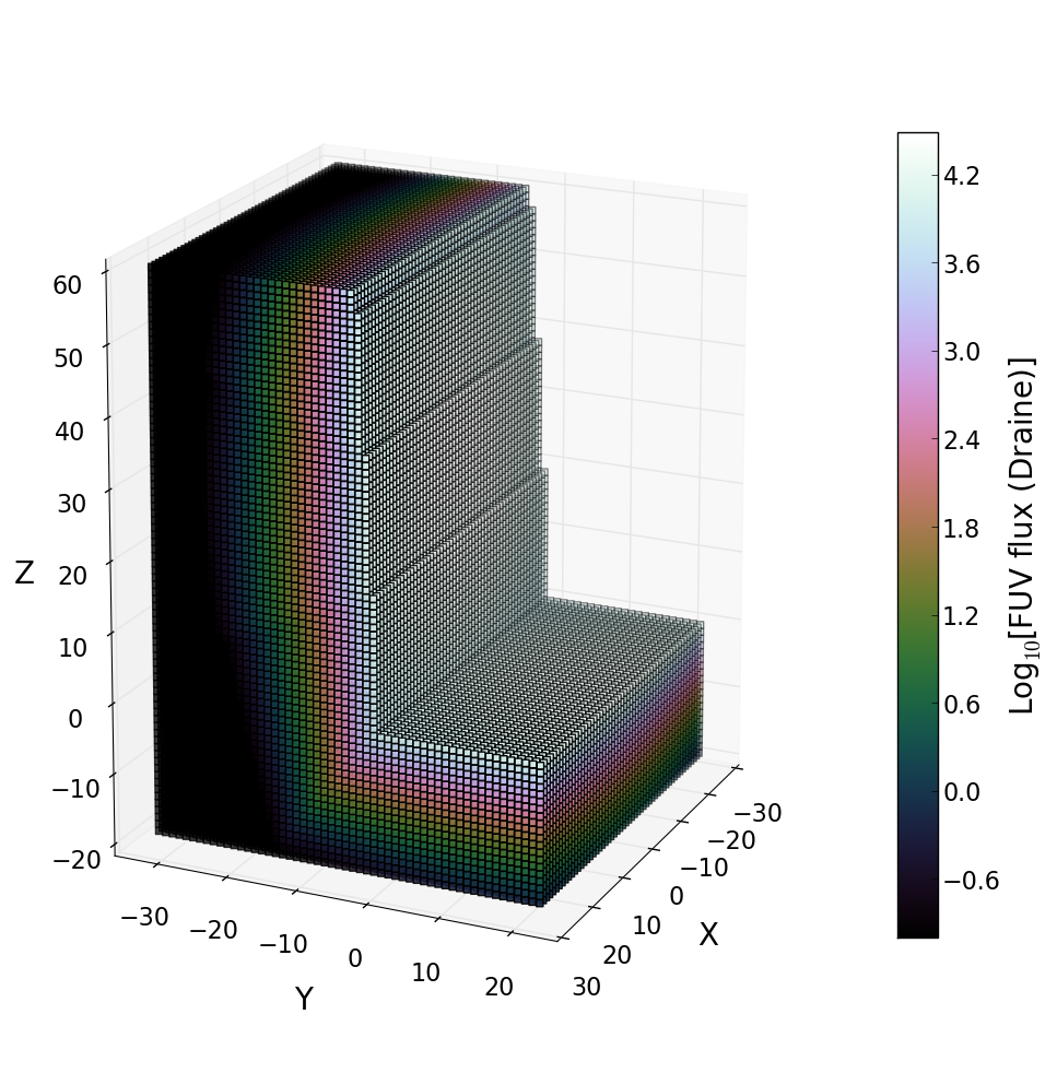
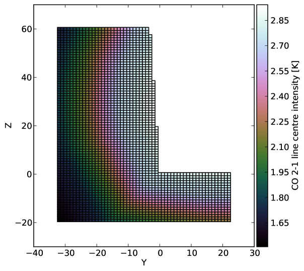
In the 3D PDR simulations the geometry of the PDR is replicated using voxels having the volume . To derive maps and spectra that are comparable to observations the radiative transfer through the 3D model needs to be calculated. An example for a 3D set-up is shown in Fig. 1 (replicating the Orion Bar PDR, which will be introduced in Sect. 3). Each small cube in Fig. 1 represents one voxel and the colour scale shows the FUV flux at the different voxels within the compound, for an FUV source located at the position .
The attenuation of the FUV photons inside the PDR is given by the sum of the optical depths, , of all voxels between the FUV source and the voxel of interest. The KOSMA- 3D code accounts for the absorption of photons and for isotropic scattering within the individual clumps (see Sect. 2.1). The code uses voxels with the shape of a cuboids, which are oriented in a way that one side of the cuboid is perpendicular to the line of sight between observer and voxel (-axis). The voxels need to be sufficiently small to trace all relevant changes of different quantities within the compound, but some compromise has to be made to reduce the overall computational effort. Therefore, the KOSMA- 3D code can make use of a set-up where the FUV attenuation is calculated for different positions within the voxels, i.e. on a 3D Cartesian grid at sub-voxel scale, and is averaged over the voxel afterwards. For each sub-voxel the code derives the line of sight that connects the centre-point of the sub-voxel and the source of the FUV radiation and evaluates which voxels intersect with this line of sight (i.e. shield FUV radiation). The FUV attenuation is weighted by the distance that is effectively crossed by a FUV photon within each voxel. The simulations presented in this work have been performed using a voxel sub-grid. For the calculation of the ensemble-averaged line intensity and optical depth (see Sect. 2.3.3), and consequently also for the radiative transfer, the sub-voxel grid is not used. This has two reasons, which are (a) while the lines of sight between the observer and a voxel are oriented perpendicular to the voxel surface, this is in general not the case for the lines of sight between the FUV source and the voxels. If we would calculate the FUV attenuation between FUV source and voxels by just summing up the between the position of the FUV source and the midpoints of the voxels we would introduce unnecessarily large errors in the case where a voxel is partly shielded by another voxel in the foreground. (b) The sub-voxel treatment is too costly for the calculation of the ensemble-averaged line intensity and optical depth where calculations need to performed at different (here: ) velocities.
We perform the radiative transfer for the same velocities that have already been used in Sect. 2.3.3. The ensemble-averaged volume emissivity and absorption coefficient, and , are calculated based on the results from the last section, Eqs. 32 and 33, i.e.
| (34) | |||||
| (35) |
where denotes the depth of the voxel along the line of sight. In the following we will omit the velocity dependence () and the “ensemble-averaged” brackets in our formulae for readability reasons.
For radiation travelling a distance along a straight path the change in intensity is given by the equation of radiative transfer, which (omitting the dependence on frequency) reads
| (36) |
Integration along a straight path length, between 0 and , yields
| (37) |
where is the background intensity of radiation travelling along the same path. For radiative transfer from voxel to the neighbouring voxel (Ossenkopf et al. 2001) and are linearly interpolated, i.e. we define and with and with
| (38) |
which can be inserted into Eq. 37 yielding
| (39) |
Eq. 39 is solved numerically and tabulated for the simulations (see Appendix B).
3 The Orion Bar PDR
The Orion Bar PDR is a prominent feature located in the Orion Nebula (M42, NGC 1976). In observations of typical cooling lines from the UV down to radio wavelength and the IR continuum the bar appears as a bright rim. With a distance of pc (Menten et al. 2007) the Orion Bar PDR is one of the nearest and hence brightest PDRs to the terrestrial observer. Consequently, a large amount of observations of the Orion Bar PDR has been performed providing us with an excellent test case for PDR models.
Chemical stratification has been observed for the Orion Bar PDR by different groups (Tielens et al. 1993; van der Werf et al. 1996; Simon et al. 1997; Marconi et al. 1998; Walmsley et al. 2000; van der Wiel et al. 2009; Pellegrini et al. 2009; Bernard-Salas et al. 2012). For example van der Wiel et al. (2009) discuss a layered structure with C2H emission peaking close to the ionisation front (IF), followed by H2CO and SO, while other species like C18O, HCN and 13CO peak deeper into the cloud.
Nowadays, it has become clear that a “simple” homogeneous (i.e. non-clumpy) bar is an insufficient description of the Orion Bar PDR. High angular resolution observations show that the bar breaks down into substructure. The commonly accepted picture is that the bar includes an extended gas component of cm-3 that causes the chemical stratification and is the dominating origin for low- molecular line emission. Embedded in this “interclump medium” a clumpy high-density ( cm-3) component is needed to provide the emission of the “high-density tracers”, among others the lines of high- CO isotopologues, CO+, and the observed H2 or OH (for a summary and additional references see Goicoechea et al. 2011). The low filling factor of the dense clumps ensures that the FUV field can penetrate deep into the cloud. We cannot list all observations that have dealt with the spatial structure of the Orion Bar. Just to name a few, Young Owl et al. (2000) presented combined single-dish and interferometric data of HCO+ and HCN which show a clumpy NE and SW bar, Lis & Schilke (2003) showed interferometric data of the Orion Bar PDR in H13CN and H13CO+ and identify at least 10 dense condensations in the H13CN image, and individual clumps have also been resolved by van der Werf et al. (1996) who showed that a PDR surface can be found on each clump inside the Orion Bar. More recent studies on the structure of the Orion Bar PDR have been performed by Goicoechea et al. (2011); Cuadrado et al. (2014).
3.1 Geometry
A common explanation for the existence of the bar is the “Blister model”: the Orion Nebula embeds a cluster of bright and young stars which ionise their surrounding medium creating an Hii-region inside the molecular cloud. At the side of the nebula facing earth this “Hii-bubble” has broken out of the cloud, enabling observations of the cavity and of the Orion Bar PDR which forms one of the edges of the cavity, illuminated by the strong FUV radiation from the young star cluster (see for example Wen & O’dell 1995 and references therein).
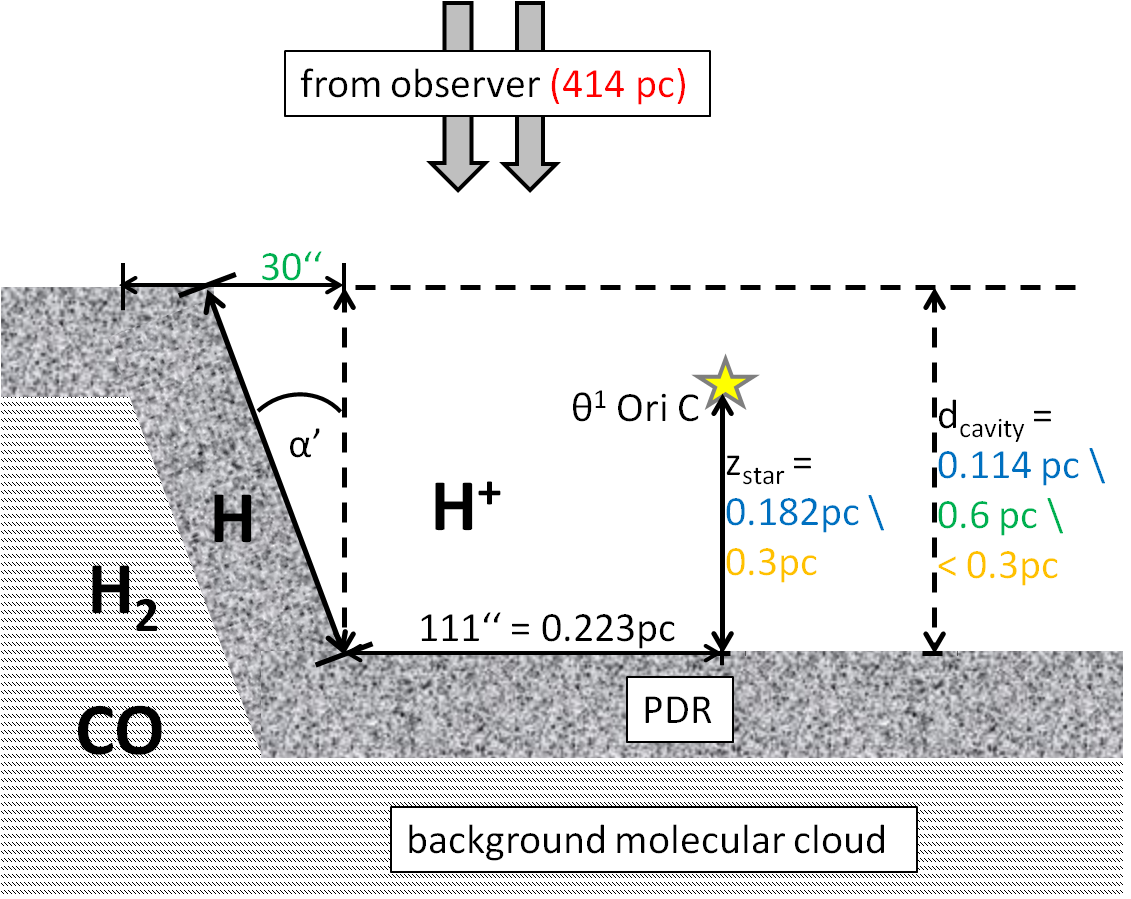
The dominating ionising source and most massive star is Ori C which produces 80% of the H-ionising photons. Ori D, the second most massive star of the “Trapezium” system, accounts for another 15% (Draine 2011). The IF, as marked for example by the peak position of the [Oii] or [Feii] emission (Walmsley et al. 2000), [Sii] (Pellegrini et al. 2009), or [Nii] (Bernard-Salas et al. 2012) is located at 111” (corresponding to 0.223 pc) projected distance from Ori C.
The flux at the IF has been estimated to correspond to an enhancement over the average interstellar radiation field, , by a factor (Hogerheijde et al. 1995; Jansen et al. 1995) (the series of papers by Hogerheijde et al. (1995) and Jansen et al. (1995) is hereafter abbreviated HJ95). We have verified that this value lies in the probable range (see Appendix C).
Different geometries have been proposed to model the Orion Bar, the dominating idea is a slightly inclined face-on/edge-on/face-on geometry first introduced by HJ95. A schematic picture of this geometry is shown in Fig. 2. Many other workgroups have used adoptions of this geometry to model observations (see e.g. Pellegrini et al. 2009). Due to the increased column density along the line of sight, this geometry naturally explains the observed intensity peak. The depth of the cavity, the inclination angle of the bar (, not to be confused with the power-law exponent from Eq. 6) and the “-position” (position on the line of sight to the observer) of the illuminating cluster have been subject to discussions. Different possibilities are indicated in Fig. 2.
The face-on/edge-on/face-on geometry is consistent with all the FIR and submm observations, but an indication that this geometry needs at least some modifications stems from optical observations (McCaughrean 2002) that show some shadowing at the very edge of the Orion Bar. This would be explained by a configuration where the Orion Bar is not the edge of a cavity but rather a filament as proposed by Walmsley et al. (2000); Arab et al. (2012).
3.2 Observations
A tremendous amount of data is available for the Orion Bar PDR. Recent observations of the Orion Bar PDR, observed with the Herschel Space Observatory (Pilbratt et al. 2010), can for instance be found in Habart et al. (2010); Goicoechea et al. (2011); Nagy et al. (2013, 2014). Recently, the whole Orion molecular cloud 1 region, which includes the Orion Bar PDR, has been mapped velocity resolved by Goicoechea et al. (2015).
As the aim of this paper focuses on the description and the testing of the KOSMA- 3D code, we selected only observations of abundant and simple species: CO isotopologues, HCO+ and the [Cii] cooling line. An expansion including many more species is of course possible.
We use [Cii], CO , CO , 13CO , 13CO and HCO+ line observations of the Orion Bar PDR observed with the Heterodyne Instrument for the Far-Infrared (HIFI, de Graauw et al. 2010) on-board the Herschel Space Observatory (Pilbratt et al. 2010). The observations have been performed as part of the EXtra-Ordinary Sources (HEXOS) guaranteed-time key program (Bergin et al. 2010). Combined with low- CO and HCO+ rotational lines (see below) these lines are well suited to trace the chemical stratification observed in the Orion Bar PDR.
The [Cii] observations have already been discussed in Ossenkopf et al. (2013). Furthermore, Nagy et al. (2014) show an HCO+ map. All other Herschel data is presented here for the first time. Further analysis of the data will be provided in subsequent papers (Choi et al. 2014, Nagy et al., in prep).
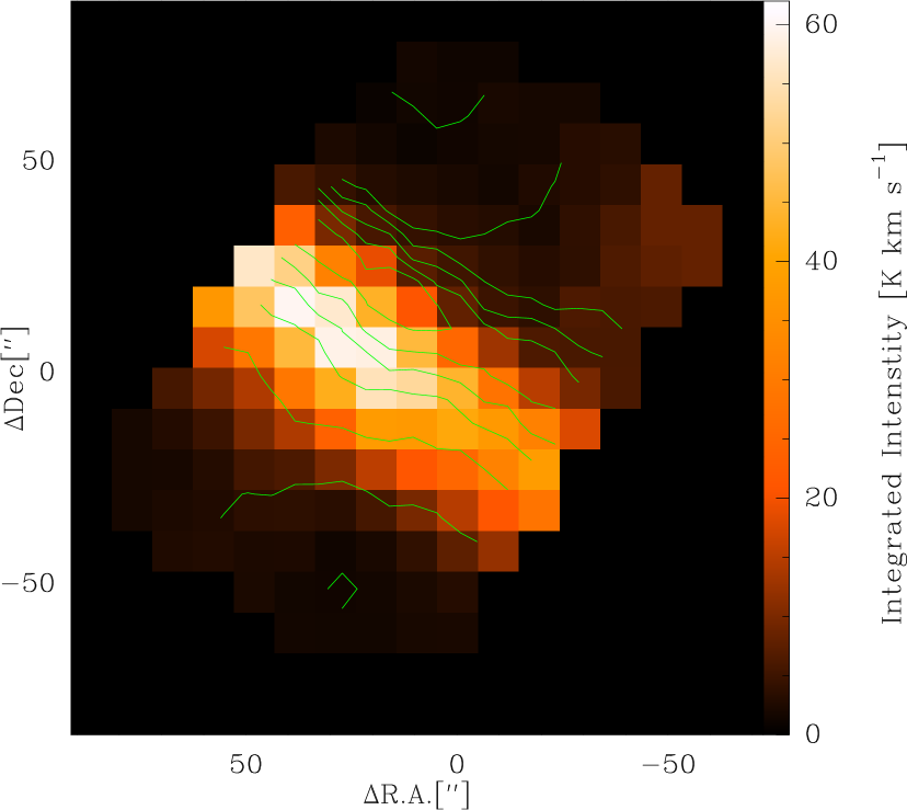
All presented HIFI/Herschel observations are strips across the bar with a width of or more, except for the CO 16-15 observations where a single cut has been observed. The observations have been taken in the on-the-fly (OTF) observing mode around the centre position ( = 5h35m20.81s, = -5∘25’17.1”) with a position angle perpendicular to the bar, i.e. 145∘ east of north, and an OFF position 6 arcminutes southeast of the map. The observations used the Wide-Band-Spectrometer (WBS) with a frequency resolution of 1.1 MHz which corresponds to 0.17 at the rest frequency of the [Cii] line. Both polarizations were averaged to improve the signal-to-noise ratio. Integration times varied between 4 and 30 s resulting in noise levels between a 0.02 and 0.3 K. The high-frequency HIFI/Herschel data, i.e. the maps of [Cii] and CO 16-15 have been reduced in HIPE as described by Ossenkopf et al. (2013). All other lines were analysed using the GILDAS software141414http://www.iram.fr/IRAMFR/GILDAS for baseline subtraction and spatial re-sampling. An overlay of our data, [Cii] overplotting 13CO 10-9, is shown in Fig. 3.
The line intensities (Table 2) are given on a scale. For the HIFI/Herschel observations is a factor 1.26 to 1.5 higher than , depending on the respective frequency (Roelfsema et al. 2012). As discussed by Ossenkopf et al. (2013), the scaling from to is questionable for very extended emission (like [Cii]) where the error beam of the telescope is likely to be filled with emission of approximately the same brightness as the main beam. Hence, for extended emission our intensities are upper limits.
Our data set is combined with ground-based observations of CO , CO , CO , 13CO , 13CO and HCO+ observed with the Caltech Submillimeter Observatory (CSO) (D. Lis, priv. comm.). The CSO observations are typically more extended but overlap with the HIFI/Herschel maps. To facilitate the comparison between the maps, the reference positions of all maps have been shifted to be equal to the CSO reference position (5h35m20.122s, -5∘25’21.96”).
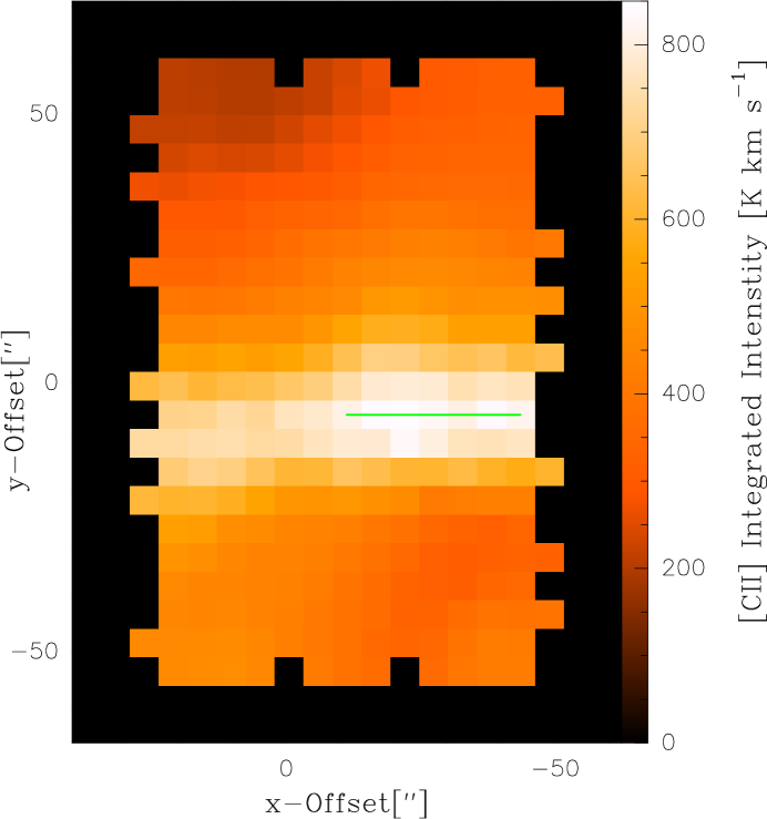
To simplify the analysis of the stratification profile, the maps have been rotated around the CSO reference position by -145∘ (-145∘ clockwise), resulting in an orientation of the Orion Bar parallel to the “-axis” (see Figs. 3 and 4). As we focus on the stratification of the chemical and excitation structure across the Orion Bar, the observed spectra have been averaged along rows of pixels151515For the CO 16-15 cut, each “row” only contains one pixel parallel to the -axis ensuring that we average over clumps and interclump medium. In the -range between and the Orion Bar has a very straight appearance in all of our maps and an average over guarantees that we are not affected by individual clumps, but consider a clump-ensemble on the observational side as well. Lis & Schilke (2003) observe the size of dense condensations in the Orion Bar and find sizes between and and Young Owl et al. (2000) discuss clumps of size, supporting our approach.
Gaussian profiles were fitted to the averaged spectra. We fit two Gaussian profiles, one profile fixed at a centre velocity of 8 km s-1 to exclude the emission from the Orion Ridge (van der Tak et al. 2013). The other profile fits the main component at about 11 km s-1 originating from the Orion Bar. Integration of this component yields the line integrated intensity, averaged for the respective row (-position). The peak position was determined by fitting a parabola to the row-averaged intensities at the different -positions. As deviations between the fitting points and the fitted parabolas are very small, we assume the pointing error of the telescope as the main uncertainty in the determination of the peak position. The pointing errors are for HIFI/Herschel (Pilbratt et al. 2010) and for CSO data161616http://cso.caltech.edu/wiki/cso/science/overview. The resulting peak intensities and -offsets are summarised in Table 2 for the different transitions. Table 2 indicates a peculiarity of the HCO+ 3–2 transition. It seems to peak in front of all the other molecular transitions, including HCO+ 6–5 that should tracer warmer gas, while the profiles of both lines are very similar. We have no evidence for a pointing problem in these data so that we stick to the formal errors, but as there is no physical scenario that would explain this peak offset we rather question the role of the HCO+ 3–2 peak position in the fit of the stratification pattern in the discussion (Sect. 5.4.1).
| Transition | Frequencya𝑎aa𝑎aTaken from “The Cologne Database for Molecular Spectroscopy (CMDS)” (Müller et al. 2001, 2005; http://www.astro.uni-koeln.de/cdms/) | Observatory | Beamsizeb𝑏bb𝑏bCalculated based on Roelfsema et al. (2012) for HIFI/Herschel. Taken from http://www.submm.caltech.edu/cso/receivers/beams.html “calculated FWHM” for CSO data. For non-circular beams an average has been used. | Peak intensityc𝑐cc𝑐cLine integrated intensity averaged along the bar at the position of the peak (see text), scale. For HIFI/Herschel the error on is about 10% (see Roelfsema et al. 2012). The error given for the CSO data has been calculated (and extrapolated for frequencies GHz) based on the errors on and given in Mangum (1993). | -offsetd𝑑dd𝑑dMeasured spatial offset into the PDR (with position angle 145∘ east of north) relative to the CSO reference position. | -offsetd𝑑dd𝑑dMeasured spatial offset into the PDR (with position angle 145∘ east of north) relative to the CSO reference position. | e𝑒ee𝑒eMeasured spatial shift into the PDR (with position angle 145∘ east of north) relative to the [Cii] peak position. |
|---|---|---|---|---|---|---|---|
| [GHz] | [arcsec] | [K km s-1] | [pc] | [arcsec] | [pc] | ||
| [Cii] | 1900.5369 | HIFI/Herschel | 11.2 | 1153 115 | -0.016 0.005 | -7.8 2.4 | 0 |
| CO | 230.5380000 | CSO | 30.5 | 402 32 | 0.029 0.006 | 14.6 3.0 | 0.045 0.008 |
| CO | 345.7959899 | CSO | 21.9 | 406 68 | 0.014 0.006 | 7.2 3.0 | 0.030 0.008 |
| CO | 691.4730763 | CSO | 10.6 | 560 244 | 0.020 0.006 | 9.8 3.0 | 0.036 0.008 |
| CO | 1151.985452 | HIFI/Herschel | 18.4 | 374 37 | 0.021 0.005 | 10.5 2.4 | 0.037 0.007 |
| CO | 1841.345506 | HIFI/Herschel | 11.5 | 128 13 | 0.019 0.005 | 9.4 2.4 | 0.035 0.007 |
| 13CO | 330.5879653 | CSO | 21.9 | 114 18 | 0.026 0.006 | 12.8 3.0 | 0.042 0.008 |
| 13CO | 550.9262851 | HIFI/Herschel | 38.5 | 120 12 | 0.042 0.005 | 20.8 2.4 | 0.058 0.007 |
| 13CO | 661.0672766 | CSO | 10.6 | 157 65 | 0.030 0.006 | 14.8 3.0 | 0.046 0.008 |
| 13CO | 1101.3495971 | HIFI/Herschel | 19.3 | 92 9.2 | 0.018 0.005 | 9.0 2.4 | 0.034 0.007 |
| HCO+ | 267.5576259 | CSO | 30.5 | 46 5 | 0.010 0.006 | 5.0 3.0 | 0.026 0.008 |
| HCO+ | 535.0615810 | HIFI/Herschel | 39.6 | 8.7 0.87 | 0.022 0.005 | 11.2 2.4 | 0.038 0.007 |
4 3D Model of the Orion Bar PDR
We have composed a 3D model of the Orion Bar PDR from cubic voxels with an edge length of 0.01 pc, corresponding to at the distance of 414 pc. The voxel size is small enough to trace physical changes in the PDR and to analyse stratification effects, but large enough to ensure that the total number of voxels can be treated on a standard PC. Furthermore, for all observations that are fitted in this work, the resulting pixel size is at least a factor two smaller than the beamsize. Our Cartesian coordinate system is chosen in such a way that the -direction is parallel to the Orion Bar and the -direction points towards the observer. As we are mainly interested in the stratification of the Orion Bar here, the current model ignores any variation of the density structure in -direction. This reduces the number of free parameters, but excludes for the moment the simulation of additional structures like the Orion Ridge.
In this work we focus on geometries for the Orion Bar PDR that are based on the HJ95 series of papers, i.e. on geometries that consist of an almost edge-on cavity wall facing the illumination from Ori C (see Figs. 1 and 2). Aiming for a fit of the observations presented in Sect. 3.2 different parameters have been varied in this model set-up. An overview over these parameters is provided in Sect. 5.1. In Sect. 5.2 we discuss the measures that are used to evaluate our fits. A second geometry that has been discussed for the Orion Bar is the filament model proposed by Walmsley et al. (2000) and Arab et al. (2012). This model consists of a cylinder in the plane of the sky with the main symmetry axis along the bar (see Fig. 27). In Appendix D we show preliminary tests of this geometry, which indicate that a simultaneous reproduction of the observed stratification pattern and the line integrated intensities based on the cylindrical model is problematic. For this geometry, the short lines of sight through the compound close to enforce that the emission peaks appear deep in the cloud, where the FUV flux is low. This reduces the line integrated intensities and increases the scatter between the -offsets calculated for the different transitions.
The main illuminating source Ori C is away from the IF. This corresponds to a separation by 22.3 voxels in -direction between star and interface. In -direction, the location of the star defines our zero point, i.e. in voxel units Ori C is located at in the model. The position of the star () is not exactly known (see Fig. 2) and has become one of our fitting parameters.
Based on C18O 3-2 observations and assuming a conversion factor of , HJ95 derive a total H2 column density of cm-2 along the line of sight (peak) for a path length of 0.6 pc. For a uniform density along the line of sight this translates into cm-3. Consequently, the total average mass in a voxel with volume (0.01 pc)3 is:
| (40) | |||||
which we use as a baseline for our simulations.
The clump ensembles in the models contain clumps at the mass points M☉, implying that one voxel typically only contains fractions of clumps, i.e. . The upper mass limit matches the resolved clump masses in the range M☉ determined for the Orion Bar PDR by Lis & Schilke (2003). The lower limit of M☉ is used as the smallest mass contained in the available KOSMA- input grid because, to gain a good approximation of a fractal geometry, the inclusion of very small structures is desired. We discuss this choice and show simulation results based on models using different mass points in Sect. 5.3.5. In the KOSMA- 3D code the pixels are scaled to superpixels (see Sect. 2.3.1). In the simulations presented here, after the scaling process, each “supervoxel” usually contains one clump at mass point M☉ and consequently for the different mass points (see Eq. 19, results rounded to integer values).
The thin interclump medium is mimicked by a second clump ensemble with an averaged density that is about two orders of magnitude lower than the averaged density of the dense clumps. To approximate a relatively homogeneous interclump medium, we start our simulations using small clumps of M☉. Furthermore, the VFF of the interclump medium should be equal to unity or smaller. Therefore, we add the condition
| (41) |
or equivalently
| (42) |
For a discussion of the interclump parameter and see Sect. 5.1. We start our simulations with a VFF of unity in Sect. 5.3.1. Different choices for the mass point and the VFF of the interclump medium are tested in Sect. 5.3.6.
In this work we do not fit the full line profiles. Therefore, the velocity spread between the clumps in one ensemble (, see Eq. 26) has been fixed. We discuss our choice of the and show examples of simulated line profiles in Sect. 5.3.7.
The KOSMA- 3D code allows for the simulation of (2D) maps. As an example, Figs. 5 and 6 show simulated maps of line integrated CO intensities, before and after the convolution with a Gaussian beam of 21.9 FWHM, matching the CSO beam used in the observations. The maps are based on model 1m (see Table 5). We find a combination of the imprint of the sharp edge of the bar and a curvature stemming from the varying distance to the illuminating star. The convolution blurs the edge and the emission peak, but still allows to recover the stratification of the emission.
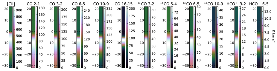
For our systematic parameter study we have reduced the map size (and the beam convolution) to a cut of only one pixel in -direction across the Orion Bar. Such a cut enables us to derive the line integrated intensities and peak offsets within a computing time of about six hours181818The computing time strongly correlates with the number of voxels used in a specific set-up. Six hours are needed for the computation on one core of a Intel® Xeon E5620 2.4 GHz CPU with 64 GB RAM.. For the 2D maps 18 days of computing time are needed. Typical simulated cuts are shown in Fig. 7 based on model 6j (see Sect. 5.3.6 and Table 5).
4.1 C18O: upper limit for the total column of molecular gas
| Transition | a𝑎aa𝑎aTelescope HPBW. | [] | |||
|---|---|---|---|---|---|
| HJ95 | 2b | 2b_ext | 6j | ||
| C18O | 13′′ | 16.1 | 38.7 | 39.4 | 35.5 |
| C18O | 21′′ | 30.2 | 41.6 | 42.2 | 37.4 |
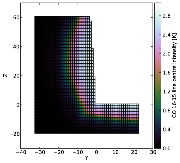
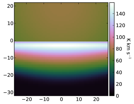
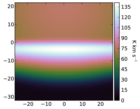
The maps of the Orion Bar can include radiation from the background molecular cloud (see Fig. 2). Therefore, we should in principle extend our model into the negative -direction until we have reached a depth were non of the investigated tracers is excited anymore. However, to reduce computing time, the background molecular cloud is cut off at in our systematic parameter study. At the FUV flux has usually dropped below one Draine field (see Fig. 1). To investigate possible contributions to the final maps/cuts from the background molecular cloud we have re-run the simulation of model 2b (which provides one of the best fits of the line integrated intensities; see Sect. 5.3.3 and Table 5), but with the compound extended to .
Figures 8 and 9 show simulated cuts through the Orion Bar model 2b, before the extension. The colour scales in these plots give the line centre intensity emitted by each voxel, in Fig. 8 for CO and in Fig. 9 for CO . The figures show that CO is only excited close to the PDR surface, where the FUV flux is relatively high. Hence, the background molecular cloud will not be visible in the final line integrated maps. For CO the situation is different: the excitation only depends weakly on the FUV flux and hence, the voxels still emit at . However, the effect of adding the background cloud to the simulation is still small due to the high optical depth of the CO line. Overall, we find that adding the background molecular cloud slightly changes the quality of the fit of the line integrated intensities (see Table 5), but it does not change the outcome of our systematic parameter study.
The total column density of the Orion Bar can be constrained from optically thin tracers that are only weakly sensitive to the PDR conditions. HJ95 provide line integrated intensities of the C18O and transitions at the emission peak of the Orion Bar PDR. Due to the low optical depths of these transitions compared to the other CO isotopologues, they provide an upper limit for the total (volume-averaged) column density of the dense clumps, including the background cloud. Table 3 compares the intensities from HJ95 to the simulated line integrated intensities based on models 2b, 6j, and 2b_ext, having cut-offs at and at . In contrast to all PDR simulations, HJ95 observed a C18O line that is significantly weaker than the line. This could be explained by a cold foreground layer. However, as we have not included foreground material into our models, a detailed fit of that line is beyond the scope of this work. Therefore, we concentrate on the C18O line for the column density estimate like HJ95.
We find that the contribution from the interclump medium to the C18O and line emission is negligible. Furthermore, the increase of the C18O line integrated intensities due to the background extension is low. Using the HJ95 column density of cm-2 leads to line intensities that are too low by more than a factor of two. Models 2b and 6j contain a mass per voxel of 2 MHJ combined with a total depth of 0.8 pc (cut-off at , parameters , , see Sect. 5.1). The total (volume-averaged) column of the ensembles of dense clumps is cm2, a factor 2.7 higher than the value that was found by HJ95. The two models provide intensities that are too high by 40 % and 25 % compared to the observations so that we consider the column density of cm2 as the upper limit. Consequently, we exclude models with higher column densities from our simulation runs. Lower columns are always allowed in our models, as they could be compensated by a deeper background cloud that is invisible in all the PDR tracer discussed here.
5 Parameter scans
5.1 Parameters
In the following we summarise the parameters that are varied within our simulation runs. If available we also give values taken from HJ95 which will be used as an initial guess for our simulations.
- :
-
The mass contained in dense clumps per voxel. Based on HJ95 we have estimated the total mass per voxel, MHJ, in Eq. 40. Furthermore, HJ95 state that about 10% (i.e. 0.1 MHJ) of the molecular material202020Atomic hydrogen is only contained in a thin surface layer () of a PDR (see for example Röllig et al. 2007). Hence, in the comparison between simulated (column) densities and the results stated in HJ95, we assume that the contribution of atomic hydrogen is negligible, i.e. we use and when comparing to the molecular densities from HJ95. is contained in clumps.
- :
-
The mass contained in the interclump medium per voxel. Following HJ95 the interclump medium accounts for 90% of the total molecular column density. Using their values, i.e. cm-3 and a total interclump mass of 0.9 MHJ in one voxel with a volume of (0.01 pc)3, the VFF is about 1.05 (see Sect. 4; per voxel this corresponds (statistically) to 0.156 clumps with a mass of M☉ and a volume of pc3). In some of the presented simulations (see Sect. 5.3.1) is no independent parameter, but coupled to to ensure an interclump-VFF of unity. Therefore, in our first simulation runs where (and ) are varied, cm-3 corresponds to MHJ (instead of 0.9 MHJ).
- :
-
The ensemble-averaged hydrogen nucleus density of the dense clumps. HJ95 derive cm-3 (i.e. cm-3) using only one type of dense clumps .
- :
-
The ensemble-averaged hydrogen nucleus density of the interclump medium. HJ95 derive cm-3 (i.e. cm-3) for a homogeneous interclump medium. In some simulations is coupled to (see above).
- :
- :
-
The z-position of the illuminating source, which is not discussed in HJ95. Here, we start our simulations using pc, i.e. with the illuminating source located at half height of the cavity.
- :
-
The FUV flux from the illuminating source, Ori C, at the position of the IF. HJ95 state . We provide an estimate of in Appendix C. The flux at a position of a voxel at the cloud surface (i.e. not affected by FUV absorptions) is given by
(43) where 0.223 pc is the observed distance in -direction between Ori C and the Orion Bar (see Sect. 3.1), is the position of the illuminating source in our model and is the edge-length of one voxel in pc.
- :
- :
-
The depth into the cloud at which dense clumps appear. With this parameter we want to test whether the same amount of clump and interclump mass is contained in each voxel, independent from the depth into the PDR, or if there is there a process that removes dense clumps from the surface. The models discussed in HJ95 do not account for such an effect, but it is proposed in the text.
- :
-
The lowest mass point of the ensemble of dense clumps. HJ95 find that a single-density model cannot explain the observed line ratios and assume that a “range of densities” appears in the beam. They construct their model with two density components (clump and interclump medium) as a “first order approximation”. Here, we start our simulations with dense clumps down to M☉.
- :
-
Mass point used for the interclump medium, i.e. the interclump medium is represented by identical clumps of mass . Here, we start with M☉.
| Parameter | Initial value | Best fit |
|---|---|---|
| [MHJ] | 0.1 | |
| [MHJ] | 0.858a𝑎aa𝑎aHJ95 find MHJ, however, we start with 0.858 MHJ for cm-3, enforcing an interclump-VFF of unity in our initial models. | 0.1…0.4 |
| [cm-3] | ||
| [cm-3] | ||
| [] | 0…3 | |
| [pc] | ||
| [pc] | ||
| [pc] | 0 | 0.02…0.04 |
| [M☉] | ||
| [M☉] |
5.2 Model assessment
To evaluate the goodness of the fit, accounting for the simultaneous reproduction of the integrated line intensities and the Orion Bar stratification structure, we determine the -position and the integrated intensity of the pixel with the highest integrated intensity for each transition from our simulated cuts.
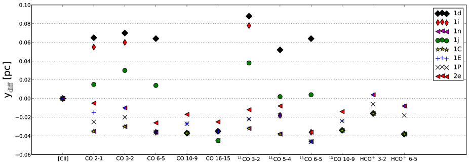
The stratification is measured in terms of the -offset of the intensity peak relative to the [Cii] peak position: where the index refers to different transitions (a negative indicates a shift towards Ori C). Simulations and observations are compared by deriving the difference between the respective offsets,
| (44) |
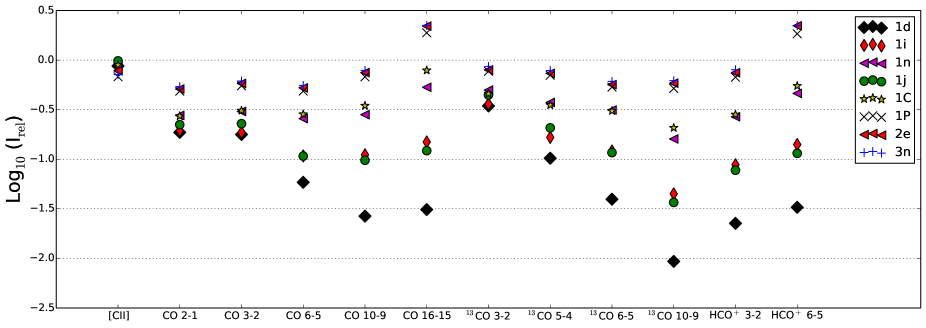
where refers to the observations (by definition, for [Cii], our reference coordinate). The relative differences between simulated and observed peak integrated intensities are given by . We summarise the and the of different models and transitions in “scatter plots” (see for example Figs. 10 and 11), which yield a clear way to compare the models and to identify systematic behaviour. In addition, we define measures to evaluate the goodness of our fits. For the -offsets we use a chi-square test, namely
| (45) |
where denotes the error of the offsets derived from the observations, as stated in Table 2, and the sum runs over all simulated transitions. A typical chi-square test, as used in Eq. 45, evaluates the model in terms of absolute (squared) differences between the observed and the fitted values. For the line integrated intensities we want a figure of merit which evaluates our models in terms of factors, for instance a simulation result that deviates from the observations by a factor two has the same quality as a results that is wrong by a factor 1/2. Therefore, we define
| (46) |
where the errors are stated in Table 2 and the denominator has been derived by error propagation, i.e.
| (47) |
When parameters are varied during the fitting process the line intensities and the -offsets are usually affected in a very different manner. To make the effects of parameter variations visible we state and separately for each simulation run. However, to evaluate how well the stratification pattern and the line integrated intensities are matched by a specific model we use the sum
| (48) |
Furthermore, the quality of a fit in the statistical sense is given by the “reduced chi-square”
| (49) |
where are the degrees of freedom (see Press et al. 1992). Here, is the number of quantities that are fitted, namely the line integrated intensities of 12 different transitions plus the 11 -offsets relative the [Cii] peak position, and is the number parameters that can be adjusted. In this work varies between different series of simulations.
The best method to derive a good fit would be to systematically explore the parameter space in all directions. Unfortunately, due to the large number of free parameters, this cannot be done within an acceptable amount of computing time. Hence, we choose the following approach: the values taken from HJ95, as summarised in Sect. 5.1, are used as an initial guess for our simulations. Successively “series of models” are run, where in each series at least two parameters are varied at a time. Based on the - test the best model from each series is selected and the parameters are kept for the next series. If there are interdependences between parameters we try to vary these parameters at the same time.
5.3 Simulation runs
| Model | VFFa𝑎aa𝑎aVolume filling factor of the interclump medium, derived from and (see Eq. 42). | b𝑏bb𝑏bDegrees of freedom used for the calculation of (see Sect. 5.2). | |||||||||||||||
| [MHJ] | [cm-3] | [MHJ] | [cm-3] | [] | [] | [pc] | [pc] | [M☉] | [M☉] | [pc] | |||||||
| 1c | 0.1 | 0.429 | 1 | 3 | 0.6 | 0.3 | 0 | 8903 | 1169 | 10072 | 504 | 20 | |||||
| 1m | 2.0 | 0.429 | 1 | 3 | 0.6 | 0.3 | 0 | 1148 | 214 | 1362 | 68 | 20 | |||||
| 1d | 0.1 | 0.858 | 1 | 3 | 0.6 | 0.3 | 0 | 8315 | 557 | 8872 | 444 | 20 | |||||
| 1i | 0.5 | 0.858 | 1 | 3 | 0.6 | 0.3 | 0 | 3642 | 356 | 3998 | 200 | 20 | |||||
| 1n | 2.0 | 0.858 | 1 | 3 | 0.6 | 0.3 | 0 | 1194 | 158 | 1352 | 68 | 20 | |||||
| 1j | 0.5 | 1.43 | 1 | 3 | 0.6 | 0.3 | 0 | 3863 | 170 | 4033 | 202 | 20 | |||||
| 1z | 2.0 | 0.0858 | 1 | 3 | 0.6 | 0.3 | 0 | 422 | 178 | 600 | 30 | 20 | |||||
| 1A | 2.0 | 0.143 | 1 | 3 | 0.6 | 0.3 | 0 | 463 | 134 | 597 | 30 | 20 | |||||
| 1B | 2.0 | 0.429 | 1 | 3 | 0.6 | 0.3 | 0 | 711 | 214 | 925 | 46 | 20 | |||||
| 1C | 2.0 | 0.858 | 1 | 3 | 0.6 | 0.3 | 0 | 1009 | 242 | 1251 | 63 | 20 | |||||
| 1D | 2.0 | 1.43 | 1 | 3 | 0.6 | 0.3 | 0 | 1248 | 151 | 1399 | 70 | 20 | |||||
| 1E | 2.0 | 0 | - | - | 3 | 0.6 | 0.3 | 0 | 323.3 | 125.7 | 449.0 | 22.5 | 20 | ||||
| 1bb | 2.0 | 0.05 | 0.035 | 3 | 0.6 | 0.3 | 0 | 291.6 | 131.4 | 423.0 | 22.3 | 19 | |||||
| 1P | 2.0 | 0.1 | 0.07 | 3 | 0.6 | 0.3 | 0 | 279.3 | 142.3 | 421.6 | 22.2 | 19 | |||||
| 1aa | 2.0 | 0.2 | 0.14 | 3 | 0.6 | 0.3 | 0 | 280 | 174 | 454 | 24 | 19 | |||||
| 2b(_ext)c𝑐cc𝑐cNumbers in brackets refer to the model extended to (see Sect. 4.1). | 2.0 | 0.1 | 0.07 | 3 | 0.6 | 0.3 | 0 | 271(266) | 131(136) | 402(402) | 24(24) | 17 | |||||
| 2d | 2.0 | 0.1 | 0.07 | 0 | 0.6 | 0.3 | 0 | 274.3 | 60.5 | 334.8 | 19.7 | 17 | |||||
| 2e | 2.0 | 0.1 | 0.07 | 0 | 0.6 | 0.3 | 0 | 272.7 | 60.5 | 333.2 | 19.6 | 17 | |||||
| 2h | 2.0 | 0.1 | 0.07 | 7 | 0.6 | 0.3 | 0 | 272 | 130 | 402 | 24 | 17 | |||||
| 2i | 2.0 | 0.1 | 0.07 | 15 | 0.6 | 0.3 | 0 | 303 | 318 | 621 | 37 | 17 | |||||
| 3a | 2.0 | 0.1 | 0.07 | 0 | 0.1 | 0.1 | 0 | 856 | 1702 | 2558 | 171 | 15 | |||||
| 3c | 2.0 | 0.1 | 0.07 | 0 | 0.3 | 0.2 | 0 | 390 | 61 | 451 | 30 | 15 | |||||
| 3n | 4.0 | 0.1 | 0.07 | 0 | 0.3 | 0.3 | 0 | 250 | 111 | 361 | 24 | 15 | |||||
| 3r | 3.0 | 0.1 | 0.07 | 0 | 0.4 | 0.4 | 0 | 252 | 93 | 345 | 23 | 15 | |||||
| 4a | 2.0 | 0.1 | 0.07 | 0 | 0.6 | 0.3 | 0 | 277 | 78 | 355 | 27 | 13 | |||||
| 4b | 2.0 | 0.1 | 0.07 | 0 | 0.6 | 0.3 | 0 | 325 | 131 | 456 | 35 | 13 | |||||
| 4d | 2.0 | 0.1 | 0.07 | 0 | 0.6 | 0.3 | 0 | 606 | 142 | 748 | 58 | 13 | |||||
| 4f | 2.0 | 0.1 | 0.07 | 0 | 0.6 | 0.3 | 0 | 280 | 126 | 406 | 31 | 13 | |||||
| 6b | 2.0 | 0.2 | 0.14 | 3 | 0.6 | 0.3 | 0.02 | 272 | 83 | 355 | 30 | 12 | |||||
| 5h | 2.0 | 0.2 | 0.14 | 0 | 0.6 | 0.3 | 0.02 | 272 | 78 | 350 | 29 | 12 | |||||
| 6a | 2.0 | 0.1 | 0.07 | 3 | 0.6 | 0.3 | 0.02 | 273 | 60 | 333 | 28 | 12 | |||||
| 6j | 2.0 | 0.2 | 0.14 | 3 | 0.6 | 0.3 | 0.04 | 285 | 31 | 316 | 26 | 12 | |||||
| 6k | 2.0 | 0.3 | 0.21 | 3 | 0.6 | 0.3 | 0.04 | 336 | 17 | 353 | 29 | 12 | |||||
| 6l | 2.0 | 0.4 | 0.28 | 3 | 0.6 | 0.3 | 0.04 | 429 | 15 | 444 | 37 | 12 |
5.3.1 Ensemble-averaged densities and masses per voxel
Each voxel within a compound is filled by two ensembles, one representing the dense clumps and one representing the interclump medium. We start our simulation runs investigating models where these ensembles are the same within each voxel (i.e. , see Sect. 5.1) and refer to these models as “homogeneous”. Examples of inhomogeneous models are given in Sect. 5.3.6.
The total mass of the clump and interclump medium contained in each voxel, as well as the related ensemble-averaged densities, have a strong influence on the simulation outcome. Especially in the homogeneous models, these parameters are interdependent: both components can contribute232323In model 1c the dense clumps do only account for 1.4% of the total FUV attenuation. In model 1m, where the total mass of the ensemble of dense clumps has been increased, 29% of the total FUV attenuation is due to this ensemble. to the FUV attenuation and hence control the line intensities emitted by both components. Therefore, we vary these parameters (, , and ) first. For all other parameters we use our initial guess (Table 4). An overview of different model set-ups is given in Table 5.
In our first series of models (represented by models 1c to 1D in Table 5) we couple to , enforcing a VFF of unity for the interclump medium. In these runs we have tested ensemble-averaged densities of , and cm-3 for the dense clumps242424An ensemble-averaged density of cm-3 combined with the four mass points implies that the smallest clumps have densities of about cm-3 (see Eq. 18). Higher densities are not possible with the current input grid (see Table 1). combined with total ensemble masses between 0.1 and 2 MHJ. As discussed in Sect. 4.1 models with MHJ (combined with pc) have been excluded. For the interclump medium we have tested densities between and cm-3, which implies total masses per voxel between 0.0858 and 1.43 MHJ. For these models the degree of freedom (see Sect. 5.2) is if a VFF of unity is enforced and if and are treated independently.
In models 1c and 1m or similarly in models 1d, 1i and 1n, the total mass of the dense clumps has been increased from 0.1 to 2 MHJ while all other parameters remain unchanged. From all tested models the parameters of model 1d are closest to the values from HJ95. Figure 10 gives an overview over the ratios between simulated and observed line integrated intensities for selected transitions. We find that the “HJ95-model” 1d does not reproduce any of the fitted line integrated intensities, except for [Cii]. However, all other intensities are too low, often by orders of magnitude. Model 1i uses the same parameters, but with Mcl,tot increased to 0.5 MHJ, which increases the line intensities of the species that are (dominantly) emitted by the dense clumps, namely the high- CO isotopologues and the HCO+ transitions. Still, the resulting line intensities are too low, except for [Cii]. In model 1n, which uses M MHJ, the line integrated intensities of most transitions are still too low, but the fit does significantly improve compared to the models discussed above.
Model 1j uses the same parameters as model 1i except for the density (and therefore also the total mass) of the interclump medium, which has been increased. In Fig. 10 one can see how the line integrated intensities of the transitions which are (at least partially) emitted by the interclump medium, namely [Cii] and the low- CO isotopologues, increase. The line intensities of the other transitions decrease due to the stronger FUV attenuation in the cloud.
Overall, we find that increasing Mcl,tot improves the quality of our fit (lower ). Furthermore, from comparing for example model 1m with 1B (or 1n and 1C; see Table 5 or Fig. 10) we find that a higher ensemble-averaged density of cm-3 provides lower and, although can increase, lower .
The spatial offsets of the different peak positions do mainly depend on the FUV attenuation in the cloud and on the peak position of the [Cii] line which is the reference for all other transitions. Figure 11 gives an overview over the (see Eq. 44) of the models that have already been included in Fig. 10. For models 1d and 1i we find that the emission peaks of the CO and 12/13CO transitions (for model 1d also of the 13CO and 12/13CO transitions) are shifted too far into the cloud by about five to nine pixels (0.05 to 0.09 pc). For model 1c (not shown, but note the high for this model) the CO and the 12/13CO emission peaks are shifted even further into the cloud, they appear about 20 pixel behind the [Cii] emission peak. Based on these transitions and for the current set-up, we have to conclude that the FUV attenuation in the cloud is significantly too weak. However, for most other transitions, the offsets are found to be too small and hence a deeper FUV penetration would be necessary to increase their -offsets. Model 1j with M and M shows a similar, but less pronounced behaviour compared to models 1d and 1i (see Fig. 11). We conclude that a fit of the stratification pattern based on the set-ups presented in this section and an interclump-VFF=1 is not possible.
5.3.2 Reduction of the interclump medium
For models 1E to 1aa the constraint that the interclump-VFF needs to be unity has been dropped. Models 1z to 1aa in Table 5 use M and cm-3. Models 1z to 1D show how the composition of the interclump medium affects the fit in terms of the chi-square tests. We find that the fit improves in terms of and if the amount and VFF of the interclump medium is reduced, allowing for a deeper FUV penetration into the cloud. The are somewhat more random, which is probably due to changing -offsets of the [Cii] reference position (see below). The models with a , i.e. models 1E, 1bb and 1P, provide similar -values and we cannot discriminate between these models based on our set-up. However, as we need to decide with which model we want to continue our simulations in the next section, we provide the with a higher precision than integer values in Table 5. Based on these results, model 1P with provides the best fit of all models discussed so far. It uses cm-3 and MHJ, resulting in an VFF of 0.07 for the interclump medium. We note that for our best fitting models the intensities of the CO and HCO+ transitions are now somewhat too high compared to the observations (see model 1P in Fig. 10).
In all models the simulated -offsets of the line peak positions of (nearly) all transitions tend to be too low. The best fit in terms of the stratification pattern () is obtained by model 1E (see Table 5). However, for this model the simulated -offsets relative to the [Cii] emission peak are too small for all simulated tracers (except HCO+ , see Fig. 11) and some transitions (12/13CO and CO ) appear at the same offset as [Cii]. Furthermore, in model 1E the interclump medium has been completely removed, while the existence of some interclump medium has been deduced from several observations. Overall, model 1P provides the best combined fit of intensity and stratification, but when we actually look at the stratification pattern it becomes clear that the fit of the pattern is not satisfactory. Good fits of the stratification pattern are only found if inhomogeneous models are used (see Sect. 5.3.6).
5.3.3 and
In a second series of simulations the effects of varying the inclination angle and the FUV flux at the cloud surface have been investigated. We have tested inclination angles of , , and , and have simultaneously increased the FUV flux by 25% and by 50% compared to the original HJ95 value. All other parameters in this second series have been adopted from the best model from the previous section, namely model 1P. As we are optimising two additional parameters in this section we use degrees of freedom for the calculation of the .
For all tested and in the tested parameter range, the fit of the line integrated intensities depends only weakly on (see for example the comparison between models 1P and 2b, where the FUV flux at the PDR surface has been increased by 50%, in Table 5). Based on the , the best fit of the line integrated intensities is provided by models 2b, 2e and 2h (, 273 and 272 respectively), which use combined with , or . These models are found to fit the line integrated intensities of all transition within a factor of about two or better, for model 2h we find and with the of all other transitions lying between these values. For models 2b and 2e the are slightly higher (see also model 2e in Fig. 10). As increasing mainly increases the line intensities of the ”outlier transitions” (see Sect. 5.4.2), we have not tested models with higher than .
Changing the inclination angle has two effects. In general, choosing a small provides more excited column along one line of sight through the compound and hence increases the line integrated intensities of the optically thin transitions. However, increasing broadens the emission peak, which can also lead to an increase of line integrated intensities after the beam convolution. Overall, we find that changing from to or has an negligible effect on the line integrated intensities, however, for the fit becomes worse (see for example model 2i in Table 5).
A more significant effect is that the fit of the stratification pattern is found to be best for , independent from the choice of . For larger inclination angles, especially for , is found to increase. The lowest is provided by model 2e, which fits the -offsets of two transitions (CO and HCO+ ) within the observational uncertainty, however, for all other transitions the simulated -offsets relative to the [Cii] peak are too small. Model 2e is also included in the scatter plots, Figs. 10 and 11.
5.3.4 and
In a third simulation run two geometrical parameters have been varied, the depth of the cavity that defines the length of the line of sight through the bar () and the -position of the illuminating source (). These parameters are partly interdependent: the column of material that is excited in the bar depends on the position of the star relative to the cavity wall. We vary both parameters, and , between 0.1 and 0.6 pc, which includes the range of values found in literature (see Fig. 2). In addition, we have investigated two models where the star is lying outside of the cavity ( pc and pc, and pc and pc). In Sect. 4.1 we have derived an upper limit for the total molecular column density along a line of sight through a model compound, which was found to correspond to MHJ for pc. Hence, for the models where has been reduced, we also test models where has been increased to provide the same upper column density limit (see for example models 3r and 3n in Table 5). All other parameters used in this section have been adopted from model 2e. For the degree of freedom we use as eight different parameters are adjusted by now.
Briefly, the result of this simulation run is that model 2e, i.e. the deep cavity ( pc) with the star at half-height ( pc) is already the best configuration. Model 3a (see Table 5) with the very shallow cavity ( and pc) can be excluded, because in this model the emission of some transitions from the back of the cavity (“below” the illuminating source) is about as strong as the emission from the bar itself. Most extremely for HCO+ the emission at of the simulated cut is significantly stronger than the emission from the bar, causing the high of this model.
For all models where the total column density of the ensembles of dense clumps is reduced compared to model 2e, the simulated line intensities decrease for all transitions, increasing the and hence decreasing the quality of the fit (see for example model 3c). On the other side, for models 3n ( pc, pc and MHJ) and 3r ( pc, pc and MHJ), which have the same column density of the dense clumps as model 2e, the fit of the line integrated intensities improves slightly compared to model 2e. This improvement stems from two effects. Placing the illuminating source close to the outer edge of the cavity puts the hottest material in the PDR closest to the observer. Therefore, after the radiative transfer, the line integrated intensities tend to be increased. Second, if the same amount of material is comprised in a shorter bar, the material is – on average – closer to the illuminating source, which increases the line integrated intensities (see Sect. 5.3.3). Therefore, the of a model with the same column density as models 3n and 3r, but with pc and , is slightly higher. However, as model 2e provides a better fit of the stratification pattern, is still has the lowest and .
5.3.5 and
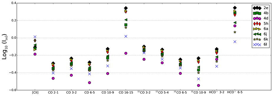
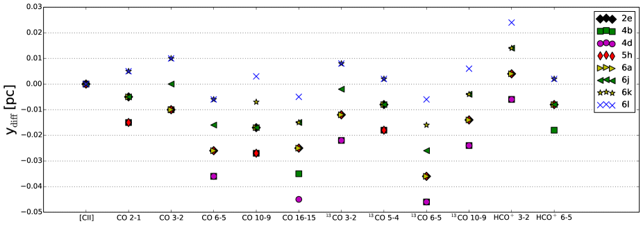
As discussed in Sect. 4, all models presented so far have used an ensemble with four mass points, M☉ (i.e. M☉), for the ensemble of dense clumps. Only the upper limit of one M☉ can be inferred from observations. Furthermore, the interclump medium was represented by identical clumps of M☉. In this section, we test the impact of these choices. For the lower cut-off mass of the ensemble of dense clumps we test M☉ and M☉ in addition to the initial value, where the second choice implies that the ensemble only contains clumps with one M☉. Each of these choices is combined with , , or M☉ for the clumps representing the interclump medium. For the degrees of freedom we use as ten different parameters have been adjusted by now.
Independent of the choice of , we find that the models that use M☉ provide the best fits. For example models 2e, 4b and 4d (see Table 5) all use M☉, but different . The of the different transitions of these models are shown in the scatter plot Fig. 12. We can see how the line integrated intensities of the different transitions systematically decrease when increases, especially CO is affected. As the line integrated intensities of all transitions except for CO and HCO+ tend to be too low, increases with increasing .
Varying the mass of the individual clumps of the interclump medium (while keeping the total mass fixed) changes the FUV attenuation and hence has an impact on the line integrated intensities and on the stratification pattern. For example for cm-3 and MHJ used in this series, decreasing from to M☉ increases the FUV attenuation per voxel by a factor 1.7, due to the more even distribution of the ISM. The line emission of the interclump medium also depends on the size of the individual clumps. Model 4f shows that, if we we increase the size of the clumps in the interclump medium, the lower emission from the interclump gas shifts the peak of the [Cii] line, strongly reducing the observable stratification. The optimal choice of depends on , however, for the models that use M☉ and hence provide the best fits, the further result clearly favour M☉. Overall, we find that model 2e, with M☉ and M☉ provides the best fit in terms of stratification and line integrated intensities.
5.3.6 Inhomogeneous models
Based on the homogeneous models used so far, the line integrated intensities can be fitted within a factor of about two for all simulated transitions. However, the homogeneous models fail in reproducing the observed stratification pattern (see discussion of models 2h/2e in Sect. 5.3.3). Furthermore, different authors (Parmar et al. 1991; HJ95; Young Owl et al. 2000) have proposed that the ISM in the Orion Bar is not uniformly distributed. Instead they present observations and models, which suggest that the inset of dense material, embedded in the thinner interclump medium, is only found at about into the cloud.
Consequently, we have tested series of models incorporating such a step. We limit ourselves to the idealised density profile that is produced if the parameter (see Sect. 5.1) is chosen to be larger than zero. Note, that for these inhomogeneous models the FUV attenuation close to the PDR surface (as defined by ) only depends on the composition of the interclump medium. The dense clumps only contribute deep in the cloud, hence the impact of varying and becomes smaller.
We have varied the parameter to be equal to 0.02, 0.03 and 0.04 pc, as suggested by the observations. As the FUV attenuation within the cloud does significantly change compared to the homogeneous models when the dense clumps are removed, we have simultaneously varied the composition of the interclump medium a second time. Therefore, we have tried values of between and cm-3 and between 0.05 and 0.5 MHJ. Furthermore, previous simulation runs have shown that for some inhomogeneous models provides better results than and hence we have repeated the simulation runs of our most promising models with instead of . In Table 5 the names of the inhomogeneous -models start with a ”5” (only model 5h is listed), while the names of the inhomogeneous -models start with a ”6”. All other parameters have been adopted from model 2e. As, compared to the models from the previous section, we have fitted one additional parameter (), we have used for the calculation of the related .
The best-fitting models of these simulation runs are (sorted for increasing and decreasing in Table 5) models 6b, 5h, 6a, 6j, 6k and 6l. We find that all of these models use between 0.1 and 0.4 MHJ combined with cm-3 and hence have VFFs of the interclump medium between 0.07 and 0.28. For these models and based on our set-up we cannot clearly discriminate between and . Models 6a, 6j, 6k and 6l provide lower -values than the corresponding -models (not shown) while model 5h is slightly better than model 6b. Furthermore, is 0.02 or 0.04 pc for these models. The observed stratification pattern is not sensitive to the exact choice.
Models 6b, 5h and 6a provide the best fit of the line integrated intensities ( or 273) of all models that have been investigated in this section, but they do not provide any improvements compared to model 2e from Sect. 5.3.3. In terms of the fit of the line intensities, the inhomogeneous model does not provide any improvement, but it also does not deteriorate the fit. The situation is very different when considering the stratification pattern. Model 6l provides , which has not been reached by any other model. In Fig. 13 we can see how for model 6l the relative -offsets lie in the pc interval for all transitions, except for the HCO+ 3-2 transition. The simulated for model 6l lie between 0.33 (13CO ) and 1.04 (CO ; see also Fig. 12).
Models 6j and 6k (see Table 5 and Figs. 12 and 13) are examples for compromises between models 2e/6b/5h/6a and model 6l. Model 6k fits the -offsets of all transitions within 0.016 pc and has between 0.4 and 1.3. For model 6j the -offset of 13CO is too small (-0.026 pc), for all other transitions the -offsets are fitted within 0.017 pc. Furthermore, the of model 6j lie between 0.46 and 1.6. Overall, model 6j provides the lowest of all models tested in the scope of this work. The simulated cuts of this model are shown in Fig. 7. In terms of a simple best fitting model, 2e is very good (2e provides the lowest ), but when explicitly asking for a reproduction of the stratification, only inhomogeneous models work. Then models 6j and 6k are much better.
5.3.7 Line Profiles
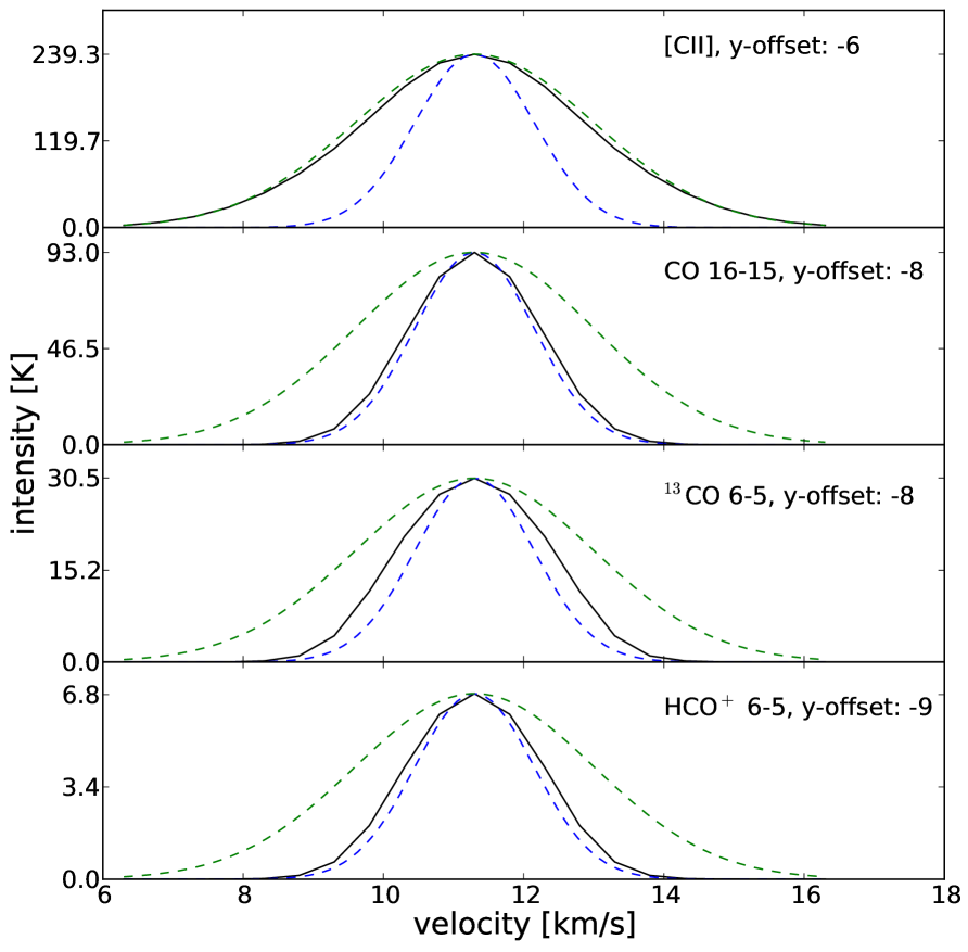
In addition to the maps and cuts presented in Sect. 4 the KOSMA- 3D code is capable of simulating line profiles for each individual pixel of a simulation. The beam convolution, which is performed by KOSMA- 3D for the line integrated intensity maps, is not applied to the line profiles. The simulation of the line profiles is based on the velocity dependent ensemble averaged line intensities and optical depths, which have been discussed in Sect. 2.3.3, and on the velocity dependent radiative transfer as discussed in Sect. 2.3.4. The line width of single clumps (, which may depend on the mass point of the individual clump, see Eqs. 27 and 28) in the KOSMA- input grid, is km s-1 (i.e. km s-1 or a Doppler broadening parameter of km s-1). The ensemble velocity dispersion (, see Eq. 26) is an additional input/fit parameter. Both, and , can be different for clump and interclump medium.
Here, we are not aiming for a fit of the line profiles observed in the Orion Bar PDR, and use a fixed velocity dispersion based on some observed line widths . For the total velocity dispersion of the dense clumps we use ( ) and for the interclump medium we use ( ) as typical values for the Orion Bar PDR (see Nagy et al. 2013 and references therein). The clump and interclump ensemble velocity dispersion then follows from
| (50) |
Consequently, our input parameters are for the ensemble of dense clumps and for the ensemble representing the interclump medium. The systematic velocity of all voxel (see parameter in Eq. 26) has been set to . Sampling the spectra at 21 different velocities around , with a spacing of km s-1 provides sufficiently smooth profiles (see velocities and in Sect. 2.3.3).
The full lines in Fig. 14 show selected line profiles from the model with the lowest , namely model 6j (see Sect. 5.3.6). The dashed lines in the figure are Gaussian line profiles with the same peak intensity as the respective profile, but with linewidths of km s-1 and km s-1, corresponding to the input linewidths. By comparing the simulated profiles with the Gaussian profiles we can see that a large fraction of the [Cii] emission is emitted by the interclump medium, while the transitions of the CO isotopologues and of HCO+ are dominantly emitted by the dense clumps. Furthermore, some profiles appear broadened as suggested by observations (Nagy et al., in prep), however, fit and quantitative comparison are left for future work.
5.4 Discussion
We find that a geometry of the Orion Bar region similar to the geometry derived in HJ95 is well suited to reproduce the observed stratification and line intensities. Significant conclusions can be drawn, however, from our unsuccessful attempts to simultaneously fit the line intensities and the peak positions measuring the geometrical stratification of the Orion Bar PDR. Initial simulations based on a cylindrical geometry (see Appendix D) are less promising.
5.4.1 The stratification pattern
The definition of based on the measurement and modelling accuracies leads to a fit that is typically dominated by the contribution of the intensity mismatches. It seems much more difficult to tweak the model towards a fit of all line intensities within the measured accuracy than towards a fit of the observed stratification pattern. Consequently, we aim for two goals that are not easily unified: on the one hand we want to provide the best fit in the statistical sense, i.e. with the lowest value of ; on the other hand we want to reproduce the observed stratification pattern as good as possible.
The lowest , namely , and hence the best fit in the statistical sense, is provided by models 2d and 2e, which fit the line integrated intensities of all transitions within a factor252525The of the different transitions lie between 0.50 and 2.1 for model 1d and between 0.51 and 2.2 for model 2e. 2.2. However, these models cannot reproduce the stratification pattern observed for the Orion Bar PDR. All models from Sects. 5.3.1 to 5.3.5 indicate that a reproduction of the stratification pattern based on a homogeneous set-up (i.e. models that contain the same ensembles of clumps in each voxel; ) is impossible.
The observable stratification in the line integrated intensity maps must stem from a combination of spatially varying excitation conditions, column densities, and line widths from clump and interclump medium (see Fig. 14 and also Fig. 27) along the different lines of sight through the inclined cavity wall, modified by the beam convolution. As the homogeneous models fail to reproduce the stratification, we had to switch to models where dense clumps only exist at some depth into the cloud; ) in Sect. 5.3.6.
This is in agreement with previous models and observations. Van der Werf et al. (1996) identify an elongated clump with a thickness of about at 20 from the IF into the cloud, and deduce a density increase in this region based on CS 5 - 4 and C34S 3 - 2 observations and a Large Velocity Gradient (LVG) model. Parmar et al. (1991) proposed already a clumpy picture of the PDR with an increasing size and number of clumps from the IF into the molecular cloud. This was later adopted by HJ95. A detailed investigation was performed by Young Owl et al. (2000). They found that the Orion Bar is best modelled when incorporating a ridge of dense clumps into a thinner interclump medium at a depth of . This is in agreement with our model fit where dense clumps have to be added to the interclump medium at a depth of to , to reproduce the observed chemical stratification.
The best fit of the stratification pattern is provided by model 6l, which has , fitting the relative -offsets within pc, i.e. in about the accuracy of the simulations, except for HCO+ 3-2. As the HCO+ 3-2 peak position provides a major outlier in the observational data (see Sect. 3.2), we rather speculate that the unsuccessful fit of this position might be caused by a problem in the observational data. For further improvements in the fit of the stratification pattern, based on our current method, higher resolution observations and smaller voxel sizes are necessary. We have also found models that provide good compromises between the fit of the stratification pattern and the line integrated intensities, overall, model 6j provides the lowest (see Sect. 5.3.6).
The parameters of the “best-fitting” models are summarized in Table 4. Our simulations show that these models can reproduce the stratification pattern, however a discrimination between the tested values for the depth at which the inset begins, , 0.03 or 0.04 pc, is not possible. The best fits of the line integrated intensities come from homogeneous models, or, if these are excluded, from models with pc. The best fit of the stratification pattern comes from a model with pc.
5.4.2 Line intensities
When using the original parameters from HJ95 (see Table 4) we find that almost all line intensities are too low compared to the observed line integrated intensities. Only the [Cii] intensity, which originates predominantly from the interclump medium, can be roughly reproduced by the original HJ95-model. Even when considering the optically thin C18O lines that were used to derive the column densities we need at least a factor 1.5 more mass per voxel than suggested by HJ95 (see Sect. 4.1). To enable a fit of the other line integrated intensities within a factor between two or three, the “best-fitting” models (see Sect. 5.4.1) use MHJ262626Or correspondingly MHJ for pc and so on. for a depth of the cavity of 0.6 pc. Consequently, our total mass per voxel is a factor 2.1 to 2.4 higher (for to 0.4 MHJ; see Sect. 5.4.4) than the value inferred from HJ95.
The difference can be explained from the nature of the different models. HJ95 use a two component (clump and interclump medium) model with a uniform kinetic temperature of K (for both components) to fit the observations. In the KOSMA- PDR code, the full gas temperature distribution is calculated as a function of the clump radius. For a clump of 1 M☉ with a hydrogen surface density of cm-3 and an FUV flux at the clump surface of , the KOSMA- PDR code computes a clump-averaged temperature of 67K, relatively close to the value by HJ95. However, in the KOSMA- simulations there is a significant change in temperature between surface and core. If we compute the average temperature “felt” by a particular molecule, i.e. obtained when weighing the temperature profile by the abundance of the different species, we obtain very different temperatures. C+, being abundant in a hot surface layer, “feels” an average temperature of about 1600K while CO and 13CO “feel” temperatures of 38K, and HCO+ of about 32K.
The emission of all optically thin molecular species is therefore significantly weaker in our model than in the 85 K model from HJ95. As the line intensities are roughly proportional to the source function, which is itself determined by the excitation temperature, we find that a change of the gas temperature from 85 K to 38 K reduces the line intensities by a factor of about 2.5 for the lower- CO lines. This explains the new upper limit on the molecular column density, deduced from the same C18O observations in Sect. 4.1, compared to the model of HJ95. By using a 2.7 times higher column density than HJ95, our best fitting model (6j) overestimates the C18O 3 - 2 line integrated intensity by about 25 % (see Sect. 4.1). This is better than the deviation that we find between our fit and observations for the other CO isotopologues. Taking the constraints from the C18O observations we cannot further increase the total column densities. However, all our model fits show the tendency that in particular the low- and mid- lines from CO, 13CO, and HCO+ are somewhat too weak.
The line integrated intensities of our best-fitting models follow a general trend, which is visible in the scatter plots, e.g. Fig. 12. While for many models the fit of the [Cii] line integrated intensity is satisfactory, it tends to be too low for other transitions, especially for CO , and and for 13CO and . Even with model 3n, which provides the best fit of the line integrated intensities, only a factor 0.54 of the observed CO line integrated intensity is reproduced (see Fig. 10). On the other side, the line integrated intensities of the CO and HCO+ transitions are predicted too high, in our best-fitting models by a factor of about two.
The numerical experiments show that the intensity of the CO and HCO+ transitions depend strongly on the FUV flux that is available for the excitation of the gas in the dense clumps. Other transitions (e.g. low- transitions of the CO isotopologues) are less affected. The FUV flux is governed mainly by the composition of the interclump medium. Due to the numerous low- line observations used within our fitting process, the models are forced into a parameter range where the interclump gas is strongly reduced, resulting in a high FUV flux within the cloud and therefore overall increased line integrated intensities. The effect on [Cii], which stems from both dense clumps and interclump gas, is minor, but for the sensitive high- rotational lines, we obtain the “outliers” with too high predictions, that have been described above. The pattern becomes even stronger when we add very small and dense clumps, i.e. when we reduce . In the opposite case, by increasing the amount of interclump medium and hence reducing the FUV flux in the cloud, we can adjust all relative intensities to similar values, i.e. remove the characteristic pattern, but then all intensities (except for [Cii]) are too low. This issue asks for a new mechanism, which systematically increases the line integrated intensities of all, in particular the low-, molecular transitions.
Adding the background molecular cloud (see Sect. 4.1 and model 2b_ext in Table 5) increases the line integrated intensities of the species that can be excited by very low FUV fluxes, i.e. of the low- transitions of the CO isotopologues and of HCO+ . Consequently, the extension of the compound improves the fit of line integrated intensities (while the influence on the stratification pattern is small) and slightly “flattens” the scatter plot of the . The amount of background material is, however, constrained by the C18O limit as discussed in Sect. 4.1, so that no significant change to our results is possible from this side.
An enhancement of the CO line intensities on the modelling site might be possible when including non-equilibrium effects due to an advancing IF: Störzer & Hollenbach (1998) find that in such models low- CO lines can be enhanced by a factor two compared to equilibrium models. The mid- CO lines can also be affected.
5.4.3 Composition of the dense clumps
The characteristic intensity pattern obtained based on the original model parameters from HJ95 (Model 1d) shows a growing discrepancy between the predicted line intensities and the observed values with the rotational level for our linear molecules. Moreover, it does not reproduce the observed stratification pattern at all. This indicates that in this set-up the molecular material is too cold and too evenly distributed. As a consequence, we had to concentrate more mass in dense clumps and reduce the fraction of interclump mass to explain the observed intensities. Apart from the need for a higher total voxel mass discussed above, a reasonable fit of the integrated intensities is only possible when increasing the fraction of material that is contained in the dense clumps from the 10% in HJ95 to 83% – 95%.
Clump densities found in the literature cover cm-3 ( HJ95, corresponding to cm-3), cm-3 (Young Owl et al. 2000) or between and cm-3 (assuming that the clumps are virialised, see Lis & Schilke 2003).
When comparing ensemble-averaged densities of cm-3 and cm-3 for the dense clumps we find that the higher density slightly improve the fit of the line integrated intensities. Unfortunately, we could not test higher ensemble-averaged densities than cm-3 due to the boundaries of the KOSMA- parameter grid. It only provided densities up to cm-3, while a full clump spectrum with an average density of cm-3 would contain some clumps with significantly higher density.
In Sect. 5.3.5, we have tested models for which the lower cut-off mass of the ensemble of dense clumps has been increased relative to the initial value of M☉. We notice that the small (and dense) clumps contribute to the molecular emission. Removing them, while keeping the ensemble-averaged density and total mass fixed, systematically decreases the line integrated intensities of all transitions (except [Cii]), especially for the high- transitions of the CO isotopologues. As the simulated line integrated intensities tend to be too low in our models, the fit of the line integrated intensities improves if small and dense clumps are included. Consequently, our simulations do not support the ”turn-over” in the clump-mass function that has been suggested by some authors (see Sect. 2.2).
For model 6j the radii of the clumps at the different mass points are pc for the ensemble of dense clumps and 0.010 pc for the interclump medium. At the distance of 414 pc to earth the size of the largest clumps ( pc) correspond to 15.8″, which is about a factor two lager than the sizes that have been observed/derived by Lis & Schilke (2003) and Young Owl et al. (2000) (see Sect. 3.2).
5.4.4 Composition of the interclump medium
The interclump medium has to account for a significant fraction of the [Cii] emission and partly for the emission of the low- HCO+, CO and 13CO lines. Its main effect is, however, the attenuation of the FUV field, effectively lowering the gas temperature in the dense clumps. Ensembles with a more homogeneous distribution of the ISM within the voxels, which is for example achieved by reducing the ensemble-averaged density while keeping the total mass constant, cause stronger FUV attenuation.
The original HJ95-parameters correspond to a VFF of the interclump medium of (nearly) unity. In a homogeneous set-up the combination of dense clumps (with MHJ) and interclump medium provides too much FUV attenuation to allow for sufficient excitation of the (especially high-) transitions that emit at some depth into the cloud. Based on simulations of inhomogeneous models with an interclump-VFF of unity (not shown) we conclude that if we limit ourselves to an interclump-VFF of one, we can fine-tune the composition of the interclump medium to optimise the fit of the stratification pattern or of the line integrated intensities, but we do not find a set of parameters providing both.
In the homogeneous set-up the fits converges towards models that use a large amount of mass in the dense clumps, but no interclump medium (see models 1z and 1E). However, such models clearly contradict the observed stratification pattern and direct observations of the interclump medium (e.g. Stutzki et al. 1988; Ossenkopf et al. 2013). If we optimise the inhomogeneous models after dropping the constraint of the fixed interclump-VFF we find the “best-fitting” models with an interclump-VFF between 0.07 and 0.28, discussed in Sect. 5.4.1.
In our initial model we used clumps of M☉ to represent the interclump medium. In Sect. 5.3.5, we varied this assumption to use clumps of M☉, M☉, and M☉ instead. Changing the mass points has two major effects. First, the mass points yield a possibility to fine-tune the FUV attenuation in the cloud. Representing the interclump medium by clumps with M☉, which allows for a more homogeneous distribution of the ISM, increases the FUV attenuation in the cloud, degrading the quality of the fit. Second, the small clumps also contribute to the molecular emission. If we increase the size of the clumps in the interclump medium, the reduced emission from the interclump gas leads to stratification offsets that are too small compared to the observed structure. Hence, our initial guess turned out to be a good choice.
For the interclump medium densities in the range cm-3 ( HJ95, corresponding to cm-3), cm-3 (Young Owl et al. 2000) or cm-3 (Simon et al. 1997) have been proposed. Our best-fitting models have a hydrogen nucleus density of cm-3. If we correct this number by the VFFs between 0.07 and 0.28 found for our best models, we obtain an average density of the interclump medium over the volume of the voxel of to cm-3, which is somewhat lower.
The Herschel observation (Fig. 3) shows that C[ii] has a rather smooth emission profile across the bar. Fig. 25 shows C[ii] emission of the interclump medium of model 6j. In this figure we have used a number surface density corresponding to 80 voxels along one line of sight, which is typical for the models discussed in this work. The figure shows that although the VFF of the interclumps medium of model 6j is only 0.04, the emission becomes rather smooth, especially if we consider that it is observed with an instrument resolution of about 0.02 pc.
5.4.5 The FUV illumination
In this work we have assumed that the FUV radiation field incident on a clump surface is isotropic. However, we have also applied the KOSMA- 3D code to the Orion Bar PDR, where the FUV irradiation comes from one dominating source, i.e. from a defined direction. Therefore, one could argue that our (isotropic) approach increases the hot PDR surface area inside the cloud leading to an overestimation of the species originating form the hot gas, for instance the high- CO lines. However, at some depth into the cloud, the FUV photons are efficiently scattered (Stoerzer et al. 1996) and the assumption of an isotropic radiation field becomes reasonable. For the description of the surface of the Orion Bar a model using beamed illumination would be more precise.
We have started our simulations with an FUV flux at the IF of , adopted from HJ95. Furthermore, in Sect. 5.3.3 we have shown how increasing this values by 25% and 50% slightly improves the fit of the line integrated intensities, but the effect is small compared to variations of other parameters. Changes of the FUV flux due to FUV attenuation inside the cloud, which is governed by the composition of the ensembles, has a significantly stronger impact on the simulation outcome. Hence, our models cannot be used to determine the FUV flux that is incident on the cloud surface.
In Sect. 5.3.4 we have presented models with inclination angels of the bar of , , or . From investigations of the line intensities emitted by the different voxels of the model compound we find that some species emit rather locally (see for example Fig. 9). For these species increasing the inclination angle can reduce the excited column density along a line of sight through the compound, into the direction of the observer. Still, an increase of the line integrated intensity in the final map is possible, due to the beam convolution. In the simulations we have to compromise between these effects. For other tracers the excitation is less dependent on the FUV flux and the emission comes from a more extended region (see for example Fig. 8). For these transitions the impact of the inclination angle is smaller. The stratification pattern is produced by the rather complicated combination between FUV attenuation, inclined geometry of the bar and beam convolution. It is difficult to disentangle these effects, however, in general the pattern becomes more random, and hence harder to fine-tune, for large inclination angles. Our best-fitting inhomogeneous models use or less. Such a small inclination angle was proposed by Melnick et al. (2012).
5.4.6 Further model improvements
As a solution to the overall insufficient fit of the line intensities of the combination of all tracers considered here, it might be useful to play with the isotopic abundances. A lower 18O abundance could potentially fit the observed high intensities of the CO and 13CO lines under the column density constraint from the C18O observations. Non-equilibrium models for the PDR chemistry as proposed by Störzer & Hollenbach (1998) could also lead to an enhancement of the CO line intensities.
To deal with the relatively high mismatch of the modelled line intensities compared to the mismatch of the stratification pattern, it may be useful to create a new chi-square criterion with a higher weight of the -offsets that allows for a better combined fit of both model aspects. Another possibility to obtain further constraints would be to fit the whole intensity profile along the cuts and not only the pixels that provide the peak intensities. A model with a more complex density structure than our idealised sharp transition might further improve our fit. Furthermore, a systematic fit of the line profiles, as discussed in Sect. 5.3.7, would provide further constraints. Important information could come e.g. from the fit to more complicated line profiles as, in the context of the Orion Bar, seen for different transitions of CH+ and SH+ (Nagy et al. 2013).
A further improvement of the fit based on the chi-square tests could come from a more deliberate selection of the fitted tracers (if available). For example, with the current selection, only [Cii] is sensitive to the thin and hot interclump gas at the IF. An inclusion of other transitions that are expected to peak at the IF, as for instance CH+ and SH+ (Nagy et al. 2013) or OH+ (van der Tak et al. 2013) could increase the weight of a correct fit of the interclump medium.
In an ideal approach we should have repeated the two-dimensional scans using different sets of initial parameters and different successions for the parameter variations, to guarantee to find the globally best fit. This was, however, practically impossible due to the relatively large computational effort for each model run. In this way our fit may not be the best possible one, but our approach guarantees that we understand the effect of every individual parameter.
6 Summary
The observation of high-density, high temperature tracers combined with a layered structure of the Orion Bar spanning over more than rules out any description of the PDR in terms of a simple plane-parallel model. PDRs, like molecular clouds, are clumpy and filamentary.
We propose a numerical model that is based on the representation of any PDR by an ensemble of clumps (possibly immersed in a thin interclump medium). Our new model ”KOSMA- 3D“ builds on the KOSMA- PDR code. It enables us to simulate the emission of star forming regions with arbitrary 3D geometries. The region is modelled using cubic voxels where each voxel is filled with clumpy structures, following a discrete mass distribution. The ensemble properties can vary between different voxels. Using a probabilistic algorithm for the calculation of the ensemble-averaged FUV extinction the incident FUV flux is derived for each voxel. A velocity dependent version of the probabilistic algorithm is used to calculate ensemble-averaged line intensities and optical depths and allows us to simulate the radiative transfer through the compound. The output of our code includes line integrated intensity maps and full line profiles.
As a first test of the new model we performed simulations of the Orion Bar PDR. In these simulations we tried to simultaneously reproduce the line integrated intensities and the spatial offsets of the emission peaks, for different transitions of CO isotopologues, HCO+ and [Cii]. Different geometries and parameter combinations have been tried out. We find that
-
•
a line fit is only possible if we invoke a process that removes dense clumps close to the PDR surface. The detailed stratification profile cannot be reproduced by models with a spatially constant ratio of clump to interclump gas.
-
•
the composition (i.e. the ensemble-averaged density and the total mass of the ensemble) of the interclump medium as well as the total molecular column density provided by the dense clumps are the most critical parameters for the simultaneous fit of the line intensities and the stratification structure of the Orion Bar. The interclump medium governs the FUV attenuation and hence the spatial layering while the clumps produce most of the emission from the molecular tracers. Our fit requires an ensemble-averaged density of cm-3 for the ensemble of dense clumps and an ensemble-averaged density of cm-3 for ensemble representing the interclump medium. Furthermore, for our best models we need a VFF of the interclump medium between 0.07 and 0.28, which indicates that also the interclump medium is not homogeneous, but breaks up into sub-structure.
-
•
to reproduce the observed line integrated intensities, a large ratio (between 5 and 20) of total clump to total interclump mass is needed. This contradicts the earlier estimates by HJ95.
-
•
The depth of the cavity and the position of the illuminating source are of minor importance, as long as the total molecular column density is fixed. Only positions of the illuminating source close ( pc) to the background molecular cloud can be excluded. Furthermore, the observations are best reproduced if a small inclination angle of the bar, in the order of , is used in the model.
The focus of this work was on testing the new 3D PDR model and on fitting line integrated intensity maps of the Orion Bar PDR. A systematic comparison of the simulated line profiles to observations is left for future work.
Acknowledgements.
We thank D. Lis for providing the CSO data and helpful comments. S. Andree-Labsch thanks the Deutsche Telekom Stiftung and the Bonn-Cologne Graduate School of Physics and Astronomy for support by means of stipends. Modelling of irradiated molecular clouds is carried out within the Collaborative Research Center 956, sub-project C1, funded by the Deutsche Forschungsgemeinschaft (DFG). Furthermore, we wish to thank the anonymous referee for his/her suggestive and detailed comments.References
- Arab et al. (2012) Arab, H., Abergel, A., Habart, E., et al. 2012, A&A, 541, A19
- Asplund et al. (2005) Asplund, M., Grevesse, N., & Sauval, A. J. 2005, in Astronomical Society of the Pacific Conference Series, Vol. 336, Cosmic Abundances as Records of Stellar Evolution and Nucleosynthesis, ed. T. G. Barnes, III & F. N. Bash, 25
- Bergin et al. (2010) Bergin, E. A., Phillips, T. G., Comito, C., et al. 2010, A&A, 521, L20
- Bernard-Salas et al. (2012) Bernard-Salas, J., Habart, E., Arab, H., et al. 2012, A&A, 538, A37
- Bisbas et al. (2012) Bisbas, T. G., Bell, T. A., Viti, S., Yates, J., & Barlow, M. J. 2012, MNRAS, 427, 2100
- Burton et al. (1990) Burton, M. G., Hollenbach, D. J., & Tielens, A. G. G. M. 1990, ApJ, 365, 620
- Choi et al. (2014) Choi, Y., van der Tak, F. F. S., Bergin, E. A., & Plume, R. 2014, A&A, 572, L10
- Cuadrado et al. (2014) Cuadrado, S., Goicoechea, J. R., Pilleri, P., et al. 2014, ArXiv e-prints [arXiv:1412.0417]
- Cubick (2005) Cubick, M. 2005, Diploma thesis, 1. Physikalisches Institut, University of Cologne
- Cubick et al. (2008) Cubick, M., Stutzki, J., Ossenkopf, V., Kramer, C., & Röllig, M. 2008, A&A, 488, 623
- de Graauw et al. (2010) de Graauw, T., Helmich, F. P., Phillips, T. G., et al. 2010, A&A, 518, L6
- de Jong et al. (1980) de Jong, T., Boland, W., & Dalgarno, A. 1980, A&A, 91, 68
- Draine (1978) Draine, B. T. 1978, ApJS, 36, 595
- Draine (2011) Draine, B. T. 2011, Physics of the interstellar and intergalactic medium (Princeton University Press), 326
- Draine & Bertoldi (1996) Draine, B. T. & Bertoldi, F. 1996, ApJ, 468, 269
- Elmegreen & Falgarone (1996) Elmegreen, B. G. & Falgarone, E. 1996, ApJ, 471, 816
- Ferland et al. (2013) Ferland, G. J., Porter, R. L., van Hoof, P. A. M., et al. 2013, Rev. Mexicana Astron. Astrofis., 49, 137
- Gierens et al. (1992) Gierens, K. M., Stutzki, J., & Winnewisser, G. 1992, A&A, 259, 271
- Glover et al. (2010) Glover, S. C. O., Federrath, C., Mac Low, M.-M., & Klessen, R. S. 2010, MNRAS, 404, 2
- Goicoechea et al. (2011) Goicoechea, J. R., Joblin, C., Contursi, A., et al. 2011, A&A, 530, L16
- Goicoechea et al. (2015) Goicoechea, J. R., Teyssier, D., Etxaluze, M., et al. 2015, The Astrophysical Journal, 812, 75
- Graham et al. (1993) Graham, J. R., Herbst, T. M., Matthews, K., et al. 1993, ApJ, 408, L105
- Green (2011) Green, D. A. 2011, Bulletin of the Astronomical Society of India, 39, 289
- Habart et al. (2010) Habart, E., Dartois, E., Abergel, A., et al. 2010, A&A, 518, L116
- Habing (1968) Habing, H. J. 1968, Bull. Astron. Inst. Netherlands, 19, 421
- Heithausen et al. (1998) Heithausen, A., Bensch, F., Stutzki, J., Falgarone, E., & Panis, J. F. 1998, A&A, 331, L65
- Hogerheijde et al. (1995) Hogerheijde, M. R., Jansen, D. J., & van Dishoeck, E. F. 1995, A&A, 294, 792
- Hollenbach et al. (2012) Hollenbach, D., Kaufman, M. J., Neufeld, D., Wolfire, M., & Goicoechea, J. R. 2012, ApJ, 754, 105
- Hollenbach & Tielens (1997) Hollenbach, D. J. & Tielens, A. G. G. M. 1997, ARA&A, 35, 179
- Hollenbach & Tielens (1999) Hollenbach, D. J. & Tielens, A. G. G. M. 1999, Reviews of Modern Physics, 71, 173
- Howe et al. (1991) Howe, J. E., Jaffe, D. T., Genzel, R., & Stacey, G. J. 1991, ApJ, 373, 158
- Jansen et al. (1995) Jansen, D. J., Spaans, M., Hogerheijde, M. R., & van Dishoeck, E. F. 1995, A&A, 303, 541
- Kamp et al. (2010) Kamp, I., Tilling, I., Woitke, P., Thi, W.-F., & Hogerheijde, M. 2010, A&A, 510, A18
- Koester et al. (1994) Koester, B., Stoerzer, H., Stutzki, J., & Sternberg, A. 1994, A&A, 284, 545
- Kramer et al. (1998) Kramer, C., Stutzki, J., Rohrig, R., & Corneliussen, U. 1998, A&A, 329, 249
- Langer & Penzias (1990) Langer, W. D. & Penzias, A. A. 1990, ApJ, 357, 477
- Le Bourlot et al. (2012) Le Bourlot, J., Le Petit, F., Pinto, C., Roueff, E., & Roy, F. 2012, A&A, 541, A76
- Levrier et al. (2012) Levrier, F., Le Petit, F., Hennebelle, P., et al. 2012, A&A, 544, A22
- Lis & Schilke (2003) Lis, D. C. & Schilke, P. 2003, ApJ, 597, L145
- Mangum (1993) Mangum, J. G. 1993, PASP, 105, 117
- Marconi et al. (1998) Marconi, A., Testi, L., Natta, A., & Walmsley, C. M. 1998, A&A, 330, 696
- Martin et al. (1984) Martin, H. M., Hills, R. E., & Sanders, D. B. 1984, MNRAS, 208, 35
- Martins et al. (2005) Martins, F., Schaerer, D., & Hillier, D. J. 2005, A&A, 436, 1049
- McCaughrean (2002) McCaughrean, M. J. 2002, in The Origin of Stars and Planets: The VLT View, ed. J. F. Alves & M. J. McCaughrean, 1
- Melnick et al. (2012) Melnick, G. J., Tolls, V., Goldsmith, P. F., et al. 2012, ApJ, 752, 26
- Menten et al. (2007) Menten, K. M., Reid, M. J., Forbrich, J., & Brunthaler, A. 2007, A&A, 474, 515
- Mertens (2013) Mertens, M. 2013, Bachelor’s Thesis, Universität zu Köln, I. Physikalisches Institut, Cologne, Germany
- Müller et al. (2005) Müller, H. S. P., Schlöder, F., Stutzki, J., & Winnewisser, G. 2005, Journal of Molecular Structure, 742, 215
- Müller et al. (2001) Müller, H. S. P., Thorwirth, S., Roth, D. A., & Winnewisser, G. 2001, A&A, 370, L49
- Nagy et al. (2014) Nagy, Z., Ossenkopf, V., Van der Tak, F. F. S., et al. 2014, ArXiv e-prints [arXiv:1405.3903]
- Nagy et al. (2013) Nagy, Z., Van der Tak, F. F. S., Ossenkopf, V., et al. 2013, A&A, 550, A96
- Offner et al. (2014) Offner, S. S. R., Clark, P. C., Hennebelle, P., et al. 2014, Protostars and Planets VI, 53
- Ossenkopf et al. (2007) Ossenkopf, V., Rollig, M., Cubick, M., & Stutzki, J. 2007, in Molecules in Space and Laboratory, ed. J. L. Lemaire & F. Combes, 95
- Ossenkopf et al. (2013) Ossenkopf, V., Röllig, M., Neufeld, D. A., et al. 2013, A&A, 550, A57
- Ossenkopf et al. (2001) Ossenkopf, V., Trojan, C., & Stutzki, J. 2001, A&A, 378, 608
- Parmar et al. (1991) Parmar, P. S., Lacy, J. H., & Achtermann, J. M. 1991, ApJ, 372, L25
- Pellegrini et al. (2007) Pellegrini, E. W., Baldwin, J. A., Brogan, C. L., et al. 2007, ApJ, 658, 1119
- Pellegrini et al. (2009) Pellegrini, E. W., Baldwin, J. A., Ferland, G. J., Shaw, G., & Heathcote, S. 2009, ApJ, 693, 285
- Pérez-Beaupuits et al. (2012) Pérez-Beaupuits, J. P., Wiesemeyer, H., Ossenkopf, V., et al. 2012, A&A, 542, L13
- Pety et al. (2007) Pety, J., Goicoechea, J. R., Gerin, M., et al. 2007, in Molecules in Space and Laboratory, 13
- Pilbratt et al. (2010) Pilbratt, G. L., Riedinger, J. R., Passvogel, T., et al. 2010, A&A, 518, L1
- Pilleri et al. (2012) Pilleri, P., Montillaud, J., Berné, O., & Joblin, C. 2012, A&A, 542, A69
- Press et al. (1992) Press, W. H., Teukolsky, S. A., Vetterling, W. T., & Flanney, B. P. 1992, Numerical Recipes in Fortran 77: The Art of Scientific Computing, 2nd edn. (New York: Cambridge University Press)
- Roelfsema et al. (2012) Roelfsema, P. R., Helmich, F. P., Teyssier, D., et al. 2012, A&A, 537, A17
- Röllig et al. (2007) Röllig, M., Abel, N. P., Bell, T., et al. 2007, A&A, 467, 187
- Röllig et al. (2006) Röllig, M., Ossenkopf, V., Jeyakumar, S., Stutzki, J., & Sternberg, A. 2006, A&A, 451, 917
- Röllig et al. (2013) Röllig, M., Szczerba, R., Ossenkopf, V., & Glück, C. 2013, A&A, 549, A85
- Simon et al. (1997) Simon, R., Stutzki, J., Sternberg, A., & Winnewisser, G. 1997, A&A, 327, L9
- Simón-Díaz & Stasińska (2011) Simón-Díaz, S. & Stasińska, G. 2011, A&A, 526, A48
- Stahl et al. (2008) Stahl, O., Wade, G., Petit, V., Stober, B., & Schanne, L. 2008, A&A, 487, 323
- Sternberg & Dalgarno (1989) Sternberg, A. & Dalgarno, A. 1989, ApJ, 338, 197
- Stoerzer et al. (1996) Stoerzer, H., Stutzki, J., & Sternberg, A. 1996, A&A, 310, 592
- Störzer & Hollenbach (1998) Störzer, H. & Hollenbach, D. 1998, ApJ, 495, 853
- Stutzki et al. (1998) Stutzki, J., Bensch, F., Heithausen, A., Ossenkopf, V., & Zielinsky, M. 1998, A&A, 336, 697
- Stutzki & Guesten (1990) Stutzki, J. & Guesten, R. 1990, ApJ, 356, 513
- Stutzki et al. (1988) Stutzki, J., Stacey, G. J., Genzel, R., et al. 1988, ApJ, 332, 379
- Szczerba et al. (1997) Szczerba, R., Omont, A., Volk, K., Cox, P., & Kwok, S. 1997, A&A, 317, 859
- Tielens & Hollenbach (1985) Tielens, A. G. G. M. & Hollenbach, D. 1985, ApJ, 291, 722
- Tielens et al. (1993) Tielens, A. G. G. M., Meixner, M. M., van der Werf, P. P., et al. 1993, Science, 262, 86
- van der Tak et al. (2013) van der Tak, F. F. S., Nagy, Z., Ossenkopf, V., et al. 2013, A&A, 560, A95
- van der Werf et al. (2013) van der Werf, P. P., Goss, W. M., & O’Dell, C. R. 2013, ApJ, 762, 101
- van der Werf et al. (1996) van der Werf, P. P., Stutzki, J., Sternberg, A., & Krabbe, A. 1996, A&A, 313, 633
- van der Wiel et al. (2009) van der Wiel, M. H. D., van der Tak, F. F. S., Ossenkopf, V., et al. 2009, A&A, 498, 161
- Visser et al. (2009) Visser, R., van Dishoeck, E. F., & Black, J. H. 2009, A&A, 503, 323
- Walmsley et al. (2000) Walmsley, C. M., Natta, A., Oliva, E., & Testi, L. 2000, A&A, 364, 301
- Weingartner & Draine (2001a) Weingartner, J. C. & Draine, B. T. 2001a, ApJ, 548, 296
- Weingartner & Draine (2001b) Weingartner, J. C. & Draine, B. T. 2001b, ApJS, 134, 263
- Wen & O’dell (1995) Wen, Z. & O’dell, C. R. 1995, ApJ, 438, 784
- Yorke (1980) Yorke, H. W. 1980, A&A, 86, 286
- Young Owl et al. (2000) Young Owl, R. C., Meixner, M. M., Wolfire, M., Tielens, A. G. G. M., & Tauber, J. 2000, ApJ, 540, 886
Appendix A Testing the probabilistic approach
In Sect. 2.3.3 ensemble-averaged line intensities and optical depths have been derived based on binomial distributions “probabilistic approach”. This formalism was verified using a direct approach that calculates the ensemble-averaged quantities for a specific realisation of an ensemble. Here, the direct approach is presented for the [Cii], CO and CO lines. As it requires a relatively large amount of computing time272727The calculation of the ensemble-averaged line intensity and optical depth of one “small” map (i.e. pixel, for instance Fig. 19) takes about two hours. it is not used in the simulations of the KOSMA- 3D code, where ensemble-averaged quantities need to be calculated for about different ensembles. However, we used it to calculate the ensemble-averaged quantities of selected ensembles with known parameters to be compared to the results of the probabilistic approach. This serves three purposes:
-
•
to verify that the ensemble-averaged quantities calculated with the probabilistic approach match the averaged quantities of real random realisations (random positions for each clump) of the ensemble.
-
•
to verify that averaging over the clump projected area (see Sect. 2.1) can be used (the method presented here accounts for the full (non-averaged) “profiles” and with being the impact parameter, or radial distance from the centre point of the clump).
-
•
to understand how much the ensemble-averaged quantities of the same ensemble can vary depending on the random positions of the individual clumps.
As discussed in Sect. 2.3.1 we consider randomly distributed clumps of masses with a fixed number surface density . The projected surfaces of the clumps may overlap. We focus on the discussion of one ensemble representing dense clumps and in addition, for the 1.9 THz [Cii] transition, we show results of one typical ensemble representing the interclump medium (see below). The “dense-clump” ensemble tested in this appendix contains clumps with masses M☉ and a total mass of 0.00346 per projected surface area (which translates into using Eq. 19). The ensemble averaged density has been fixed to be cm-3, the averaged densities of individual clumps have been calculated using Eq. 18.
As discussed in Sect. 2.3.1 a clumpy ensemble can be scaled to arbitrary numbers of clumps as long as the number surface density for each mass point, , is kept constant. For the direct approach we create squared maps of a size in which the (centre points of the) clumps are randomly distributed. Two different map sizes are used in this appendix, “small” maps contain one and “large” maps contain two clumps at mass point 1 M☉. In the maps we ignore an area of the thickness around the edges because that region could be affected by clumps with centres outside of the map, that are no taken into account here.
Maps282828For all presented maps an FUV flux of has been used. of random representations of the ensemble of dense clumps are shown in Figs. 15, 16, 19 and 21. For instance, the colour scale of Fig. 15 shows the line centre intensity of the [Cii] line, summed up along lines of sight perpendicular to the printed surface. [Cii] emission is strongest in the outer layers of the clumps. It is affected by limb brightening. The resulting “intensity profile” (see Eq. 5), where the [Cii] line intensity is highest at the edge of each (sufficiently large) projected clump, is clearly visible in Fig. 15. Analogously to Fig. 15 “optical depth maps” have been simulated. For example Fig. 16 shows the same map as Fig. 15 but with the colour scale giving the optical depth of the [Cii] transition.
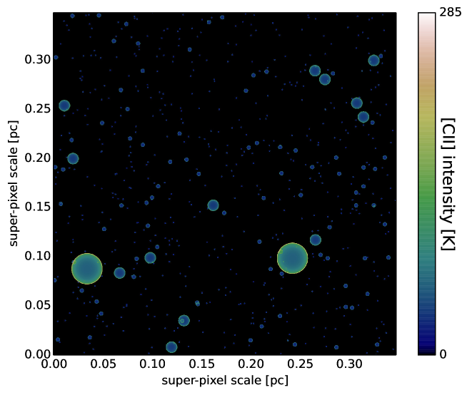
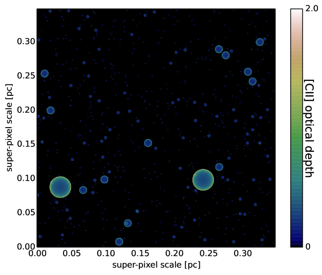
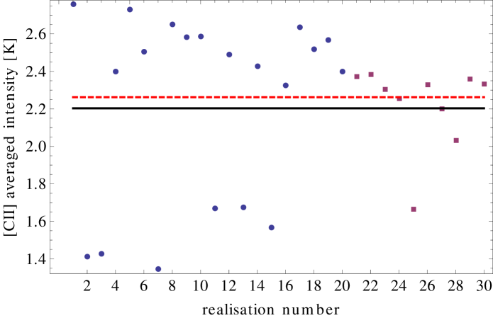
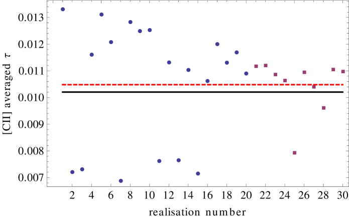
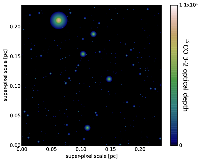
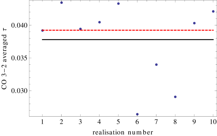
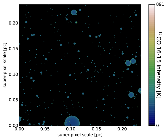
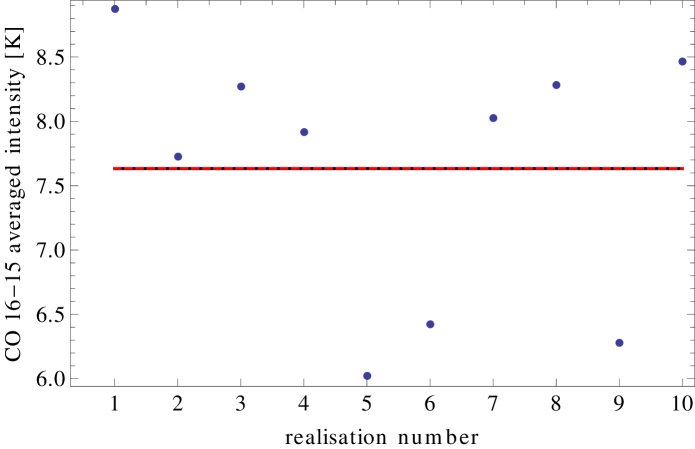
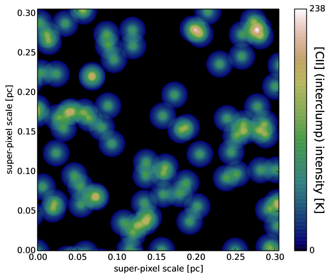
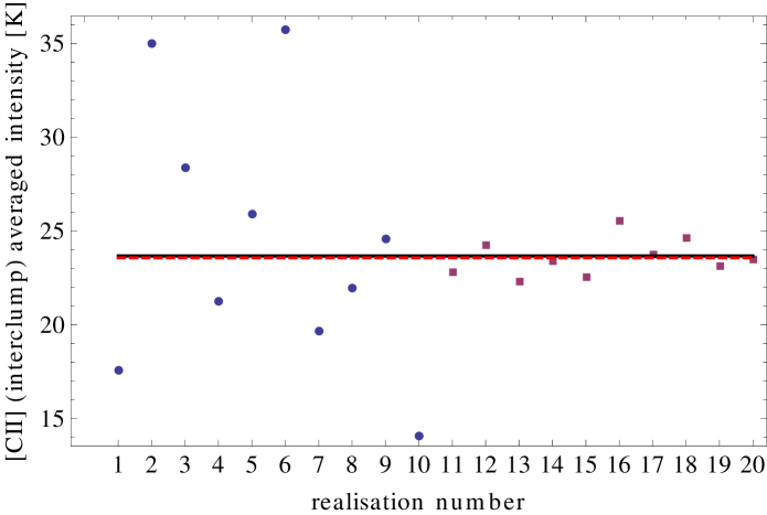
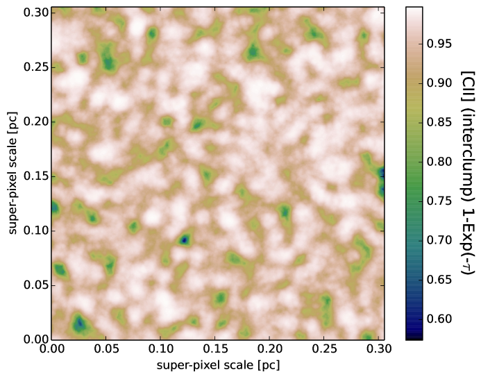
Each map has been derived on a spatial grid with a grid-spacing (see Sect. 2.3.1). The large maps, for instance Fig. 15, contain grid points while the small maps (see Figs. 19 and 21) contain grid points. For each map the ensemble-averaged quantities are calculated using
| (51) | ||||
| (52) |
where the index denotes different gridpoints. The resulting and can be compared to the results from the “binomial” approach (Eqs. 54 and 55).
In the presented comparison we account for only one velocity bin with centre-velocity . This velocity bin contains all clumps of the ensemble and Eq. 26 simplifies to
| (53) |
Furthermore, due to , Eqs. 27 and 28 simplify to
| (54) | ||||
| (55) |
giving the line-centre intensity and optical depth for each combination of clumps. As we do not have to sum up contributions from different centre-velocities, the ensemble-averaged quantities are provided by Eq. 2.3.3 and 2.3.3, for . These will be compared to the results from the probabilistic approach.
For the [Cii] line the ensemble-averaged line intensity and optical depth have been derived for 30 different realisations of the ensemble including 20 small and 10 large maps. The results are summarised in Figs. 17 and 18 for the intensities and optical depths, respectively. As expected, the averaged values calculated for single realisation in Figs. 17 and 18 show some scatter, which is larger for the smaller maps (this effect is better visible in Fig. 24 where the size-difference between the maps is larger). The scatter shows us how much single representations of the ensemble, which might exist in molecular clouds, can differ from the mean value derived with the probabilistic approach. The black lines give the line intensity or optical depth averaged over the 30 results of the individual representations. Within this calculation the maps got different weights, proportional to their respective sizes. The red, dashed lines show the ensemble-averaged quantities for the same ensemble, calculated using the probabilistic approach. For [Cii] the two approaches agree within 2.6% for line intensities and optical depths.
The reliability of the approach presented here depends on the size of the calculated maps and on the number of representations of the ensemble to be averaged over. However, a statistical difference remains between simulating one very large map or several smaller maps with the same total size. This difference can be understood from the different [Cii] maps: while for the large maps with (for example) a clump at the highest mass point can overlap with a clump of the same kind, this overlap is not possible for the small maps with . However, Fig. 17 shows that this difference is negligible for the dense ensembles in this work, due to their small area filling factors. For the interclump medium, which has a higher area filling factor, the situation is different (see below).
For each CO line 10 small maps have been analysed. Fig. 19 shows such a map with the optical depth of the CO transition given on the colour scale. As expected the CO optical depth is highest for lines of sight intersecting with the dense cloud cores. The related statistical overview is shown in Fig. 20. We find that the two approaches agree within 3.7% (3.5%) for the optical depths (line intensities). Possibly, increasing the number of samples could improve this result.
For the CO 16-15 line we present an “intensity map” in Fig. 21 and the related statistical overview in Fig. 22. The map (Fig. 21) shows the 5th realisation of the ensemble from Fig. 22. Here, the large clump is sitting at the lower edge of the map and is partly cut away causing the small ensemble-averaged intensity (and optical depth). However, this situation is part of the “normal” statistics. For CO the agreement between the two approaches is excellent (which is coincidental due to the rather low number of sample maps), we find deviations between the two approaches of 0.004% and 0.8% for line intensities and optical depths, respectively.
In addition to the ensemble of dense clumps we test one “typical” interclump-ensemble. This ensemble contains clumps at one mass point ( M☉), a total ensemble mass of M☉ per projected surface area, and an ensemble averaged density of cm-3. It has an area filling factor (, i.e. not accounting for the fact that clumps do overlap) of about 0.8. The clumps are lying on a gridpoint of the KOSMA- model grid, making interpolations unnecessary. One representation of this ensemble is shown in Fig. 23 where the colour scale gives the [Cii] line (centre) intensity. The map originally contained 100 identical clump, a few clumps have been cut away during the removal of the edges of the map. Note that for this ensemble the clumps at mass point M☉ are about a factor six larger compared to the previous ensemble, due to the reduced density. The [Cii] intensities of different realisations of the ensemble, for maps that contained initially 10 or 100 clumps, are shown in Fig. 24. The comparison to the probabilistic approach292929For the interclump medium the probabilistic approach yields an ensemble-averaged [Cii] line centre intensity of 23.68 K for and of 23.57 K for . shows that the deviation between the two results lies below 1% for line intensities and optical depths.
The excellent agreement between the two approaches for the interclump ensemble indicates that averaging over the projected surface (see Sect. 2.1) hardly introduces any error. Furthermore, the interpolation between the line profiles and , as needed for the ensemble of dense clumps during the analysis with the direct approach, does not cause large deviations. All compared results are found to agree within the statistical scatter, which is quantified by the standard deviations of the scatter of the ensemble-averaged quantities, calculated with the direct approach.
In addition to the ensembles used for the statistical analysis in this section, we have added Fig. 25, which shows clumps based on the parameters of the interclump medium of model 6j (see Table 5), with a number surface density corresponding to 80 voxels along a line of sight. This figure is further discussed in Sect. 5.4.4.
Appendix B Numerical handling of the radiative transfer
A solution of the equation of radiative transfer, based on linear approximations of the emission and absorption coefficient, has been presented in Sect. 2.3.4. Here, we discuss the numerical handling of the integral in Eq. 39 in the KOSMA--3D code. The numerical integrations in this section were performed using Wolfram Mathematica303030http://www.wolfram.com/mathematica/.
Before we solve the integral in Eq. 39 we need to distinguish three different cases:
-
1.
If no absorption takes place between two pixels, i.e. and , the equation of radiative transfer (Eq. 36) reduces to
(56) and integration between 0 and yields
(57) where indicates the incident background emission. Note that this case (i.e. an infinite source function and hence an infinite excitation temperature) cannot occur in any physical source. However, in the code it is needed if there are “holes” in the set-up i.e. if voxels on a line of sight are not occupied by an ensemble (at a specific velocity) or for artificial sources which have been constructed in a way that voxels emit at a specific frequency without absorbing it. Practically, in the code, the condition and has been used for this case, avoiding errors due to numerical inaccuracies.
-
2.
If the absorption coefficient does not change between two pixels, i.e. but , Eq. 39 reduces to
(58) and numerical integration yields
(59) Practically, in the code, the condition has been used for this case.
-
3.
The third case is the general case which is always used if . Numerical integration of Eq. 39 yields
(60) with
(61) where denotes the imaginary Error Function. is further discussed below.
Implementation, runtime and precision of the imaginary error functions in Eq. 61
are problematic
for large function values. In the code this is avoided by the following rearrangements and substitutions:
The function , Eq. 61, can be written as
| (62) | ||||
with
| (63) | |||
The function has been constructed in a way that (subtractions between) large numbers are avoided. It is different for and . Furthermore, it can be approximated for large and small function values. For it is given by
| (64) |
for (and consequently imaginary a and b) it is given by
| (65) |
For both functions, Eqs. 64 and 65, have been tabulated. The code interpolates linearly between the tabulated values. Note that maser lines (, i.e. ) are treated in linear approximation. Hence, the code should not be used for strong maser lines. For all other , including weak maser lines ( with ), the relative error made by interpolation or approximation of is less than one percent.
Appendix C FUV flux at the ionisation front
Jansen et al. (1995) state that the radiation field incident on the Orion Bar corresponds to an enhancement over the average interstellar radiation field, , of a factor . Other authors give similar values, Marconi et al. (1998) estimate a flux of times the average interstellar field. Arab et al. (2012); Young Owl et al. (2000); Walmsley et al. (2000) used at the IF with being the Habing field (Habing 1968)313131The ratio between the Draine field and the Habing field (both integrated over the FUV range) is (Draine & Bertoldi 1996)..
Here, we have re-estimated the FUV flux at the IF, originating from Ori C, based on synthesised stellar spectra provided by Martins et al. (2005)323232Available online: http://www.mpe.mpg.de/~martins/SED.html. Different spectra from their sample have been investigated, for stars having effective temperatures between 35000 and 39540 K which covers the spectral classes from O7V to O6V. Different authors (Stahl et al. 2008; Pellegrini et al. 2009; Arab et al. 2012) obtained varying results for the spectral class of Ori C, all falling in the range between O6 and O7.
The selected spectra have been integrated in the FUV range, 2066 to 911 Å (6 to 13.6 eV), and the resulting flux at the position of the Orion Bar has been computed. For this calculation, the distance between Ori C and the Orion Bar has been assumed to be 0.223 pc, i.e. equal to the projected distance (neglecting a possible offset in radial direction which is not precisely known, see Sect. 3.1). The calculated fluxes fall between 17 and 373 erg s-1 cm-2 ( ), covering the range of values discussed above.
The FUV flux representative for an O6.5 star ( K, Martins et al. 2005) is found to be 38 erg s s-1 cm-2 or at the IF. The flux of from HJ95 is best reproduced by the star from the sample with K, which indicates the spectral class O6.5V (Martins et al. 2005). The calculated FUV fluxes make strong FUV absorption inside the Hii region between star and PDR improbable in agreement with the lack of dust observed in the cavity. Dust must have been blown out by the strong stellar winds.
Appendix D Cylindrical models
| Name | parameters adopted from | |||
|---|---|---|---|---|
| Cyl. 1 | 1z | 602 | 120 | 722 |
| Cyl. 2 | 1A | 674 | 201 | 875 |
| Cyl. 3 | 2b/2e/2h | 336 | 79 | 415 |
| Cyl. 4 | 6b | 419 | 66 | 485 |
| Cyl. 5 | 6j | 515 | 59 | 574 |
| Cyl. 6 | 6k | 648 | 74 | 722 |
| Cyl. 7 | 6l | 825 | 50 | 875 |
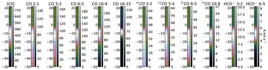
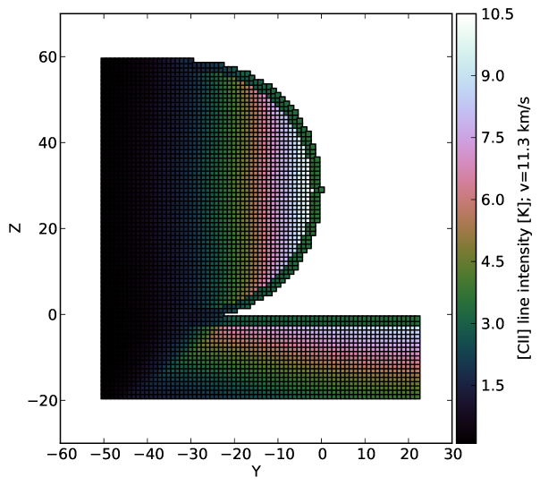
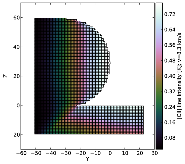
As discussed in Sect. 4 we have also tested models where the Orion Bar has a cylindrical shape (see Figs. 27 and 28). The tests of this geometry are based on the assumption that the sets of parameters that provide the best simulation results for the HJ95 geometry are also good initial guesses for the cylindrical model. We use a cylindrical model with a deep cavity, pc, and hence a radius for the cylinder of 0.3 pc. The centre point of the cut through the cylinder is and the illuminating source is located at (see Fig. 27). The inclination parameter is not needed for a cylinder. Table 6 gives an overview over some cylindrical models. The second column of the table refers to the corresponding model from Table 5 for the remaining parameters, i.e. the composition of the clump ensembles, and .
Figures 27 and 28 show cuts through the cylindrical model Cyl. 4, which is an inhomogeneous model with pc. The colour scales give the [Cii] line intensity emitted by the dense clumps and the interclump medium of the respective voxel at a specific velocity, Fig. 27 shows the line-centre intensity (at 11.3 ) and Fig. 28 the emission in the line wing (at 8.3 ). The Fig. 27 illustrates that at the line centre velocity the [Cii] emission is dominated by the dense clumps, that only start two voxels below the cloud surface. Due to the higher velocity dispersion of the interclump medium (see Sect. 5.3.7), the 8.3 channel in Fig. 28 is dominated by the [Cii] emission from the interclump medium, providing the highest line intensities in the voxels that are closest to the illuminating source. The observable stratification pattern follows from the radiative transfer and the beam convolution of these pictures.
In general, for cylindrical models the -offsets where the line integrated intensity peaks for the different transitions are shifted deeper into the cloud (into the negative -direction) compared to the corresponding cavity-wall models. For all models listed in Table 6 the [Cii] line integrated intensity peak (i.e. the reference positions for the -offsets) is shifted by one to three pixels deeper into the PDR compared to the cavity-wall model with the same parameters. As an example Fig. 26 shows the simulated cuts of model Cyl. 5. Here the [Cii] peak lies at pc, while the peak appears at pc in model 6j. Hence, to provide a stratification pattern, the -offsets of all other transitions need to be shifted even deeper into the cloud in the cylindrical models. This is hardly observed. The line intensity is dominated by the column density along the line of sight given by the cylindrical geometry, less by changing composition or excitation conditions. For the cylinder the lines of sight through the compound close to are shorter than the lines of sight through the cloud material in the cavity-wall set-up (assuming small ). Therefore, the peaks are moved away from the edge of the cloud in the cylindrical model, to positions where the lines of sight through the compound and hence the column densities are larger. This leads to the higher -offsets.
Depending on the specific model set-up, the can decrease or increase when we switch from the cavity-wall models to the cylindrical geometry. However, this comparison is ambitious, as the of the HJ95-models also depend on the inclination angle . Similar to the HJ95-models we find that the fit of the stratification pattern is better when an inhomogeneous model (i.e. models Cyl. 4 to Cyl. 7) is used, compared to the homogeneous set-ups (models Cyl. 1 to Cyl. 3). Non of the homogeneous models can reproduce any stratification for the CO transition. Models Cyl. 5, 6 and 8 do provide peak positions relative to the [Cii] peak (see Sect. 5.2) for all transitions. However, the scatter around the observed values, complicating the fine-tuning of the stratification pattern. Non of the tested models reaches the of our best HJ95-models.
With the parameters from Table 5 the cylindrical geometry provides always systematically lower line integrated intensities for all transitions than the cavity-wall model, resulting in a deteriorated fit (in terms of the ). This reduction results from a combination of two effects: (a) shorter lines of sight and hence reduced column densities at the front of the cylinder, (b) less FUV flux available for the excitation when the peaks are shifted deeper into the cloud (see above). This already shows the fundamental problem of cylindrical models.
Consequently, we find that the fits based on the tested cylindrical model do not reach the quality (in terms of the ) of the HJ95- models. Of course these results could be improved if step-by-step fine-tuning of the parameters is performed, however, fine-tuning of the stratification patter is expected to be difficult due to the scattering of the of the different transitions. An improvement of the fit of the line integrated intensities might be possible if the mass per voxel in the dense clumps is drastically increased, leading to larger molecular column densities close to . A cylinder with less curvature might also provide better results.