Singular spin-wave theory and scattering continua in the cone state of Cs₂CuCl₄

Abstract

For temperatures below $0.6\,\text{K}$ the geometrically frustrated layered quantum antiferromagnet Cs₂CuCl₄ in a magnetic field perpendicular to the layers orders magnetically in a so-called cone state where the magnetic moments have a finite component in the field direction, whereas their projection onto the layers forms a spiral. Modeling this system by a two-dimensional spatially anisotropic quantum Heisenberg antiferromagnet with Dzyaloshinskii-Moriya interaction, we find that even for vanishing temperatures the usual spin-wave expansion is plagued by infrared divergencies which are due to the coupling between longitudinal and transverse spin fluctuations in the cone state. Similar divergencies appear also in the ground state of the interacting Bose gas in two and three dimensions. Using known results for the correlation functions of the interacting Bose gas, we present a nonperturbative expression for the dynamic structure factor in the cone state of Cs₂CuCl₄. We show that in this state the spectral line shape of spin fluctuations exhibits singular scattering continua which can be understood in terms of the well-known anomalous longitudinal fluctuations in the ground state of the two-dimensional Bose gas.

I Introduction

The magnetic insulator Cs₂CuCl₄ is one of the few known physical realizations of a spin system where the combined effect of geometric frustration and strong spin fluctuations can stabilize the spin-liquid phase in a substantial range of temperatures $T$ and external magnetic fields $H$, see Ref. [Balents, 2010] for a recent review. The phase diagram of Cs₂CuCl₄ as a function of $T$ and $H$ has been thoroughly mapped out using various experimental techniquesColdea et al. (2002, 2003); Sytcheva et al. (2009); Kreisel et al. (2011); Vachon et al. (2011) and comprises paramagnetic, spin-liquid, and magnetically ordered phases. The spin liquid phase, which for vanishing magnetic field is observed in the temperature range $0.6$ K $<T<2.6$ K, has received a lot of attention from theory.Starykh and Balents (2007); Kohno et al. (2007); Balents (2010); Starykh et al. (2010); Griset et al. (2011); Chen et al. (2013); Herfurth et al. (2013) On the other hand, it seems to be generally accepted that the magnetically ordered low-temperature phase of Cs₂CuCl₄ in an external magnetic field along the crystallographic $a$ axis is rather conventional. For this direction of the magnetic field, the magnetic moments in the ordered phase form a so-called cone state (also called umbrella state), where the moments have a finite projection onto the direction of the field, whereas their projection onto the plane perpendicular to the field forms a spiral, as shown in Fig. 1.

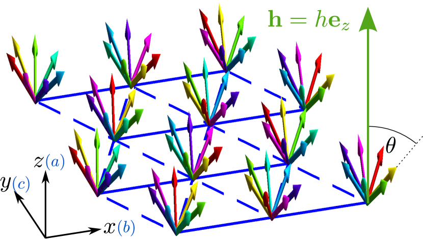
Figure 1: (Color online) Graphical representation of the spin configuration in the cone state, which is the ground state of Cs₂CuCl₄ in a magnetic field $\bm{h}=h\hat{\bm{z}}$ pointing along the crystallographic $a$ axis. An explicit expression for the spin configuration in the cone state is given in Eq. (5). In the figure, a set of arrows with the same color represents the cone state with incommensurate ordering vector $\bm{Q}$ where the spins are tilted towards the magnetic field ($\theta/\pi=0.35$ in the figure). Different colors show the other possible states for the same value of the magnetic field that differ only by a gauge transformation of the magnetic order parameter.

We will show in this work that in this phase the usual spin-wave expansion is plagued by infrared divergencies. At the first sight, this is rather surprising, because for a two-dimensional spin model the usual phase space arguments (which are employed in the proof of the Mermin-Wagner theoremMermin and Wagner (1966) to rule out the existence of long-range magnetic order at finite $T$) do not imply any divergencies at $T=0$. We show that the infrared divergencies encountered in the cone state of Cs₂CuCl₄ have a different physical origin: They arise from the coupling between longitudinal and gapless transverse spin fluctuations. In fact, similar divergences are encountered in the theory of the interacting Bose gas where interaction corrections to Bogoliubov’s celebrated mean-field theory for the condensed phase are known to be infrared divergent in two and three dimensions.Nepomnyashchii and Nepomnyashchii (1978); Popov and Seredniakov (1979); Weichman (1988); Giorgini et al. (1992); Castellani et al. (1997); Pistolesi et al. (2004) Note, however, that these divergencies do not arise in the spin-wave expansion of many other quantum magnets because spin conservation forces this coupling to vanish in the long wavelength limit. Fortunately, in the Bose gas nonperturbative resummations of these divergencies are available, leading to a nonanalytic contribution to the longitudinal part of the bosonic two-point function.Sachdev (1999); Zwerger (2004); Kreisel et al. (2007); Dupuis (2011) In this work we will apply these results to the cone state of Cs₂CuCl₄ and show that they imply the existence of extended scattering continua on the spin dynamic structure factor in a magnetic field. A similar strategy has been adopted previously in Ref. [Kreisel et al., 2007] to calculate the dynamic structure factor of a quantum antiferromagnet in a uniform magnetic field.

The minimal model for describing the cone state in Cs₂CuCl₄ is the following two-dimensional antiferromagnetic Heisenberg model in an external magnetic field along the crystallographic $a$ axis (which we identify with the $z$ axis of our coordinate system)

$${\cal{H}} =\frac{1}{2}\sum_{ij}\left[J_{ij}{\bm{S}}_{i}\cdot{\bm{S}}_{j}+\bm{D}_{ij}\cdot({\bm{S}}_{i}\times{\bm{S}}_{j})\right]-h\sum_{i}{{S}}^{z}_{i}.$$ (1)

Here the sums are over all $N$ sites of the lattice, and $h=g\mu_{B}H$ is the Zeeman energy associated with the magnetic field $H$, where $g\approx 2.19$ is the effective Landé factorColdea et al. (2002) and $\mu_{B}$ is the Bohr magneton. The spin operators $\bm{S}_{i}=\bm{S}(\bm{R}_{i})$ satisfy $\bm{S}_{i}^{2}=S(S+1)$ with $S=1/2$ and are localized at the sites $\bm{R}_{i}$ of a distorted triangular Bravais lattice with crystallographic lattice constants $b$ and $c$ as shown in Fig. 2.

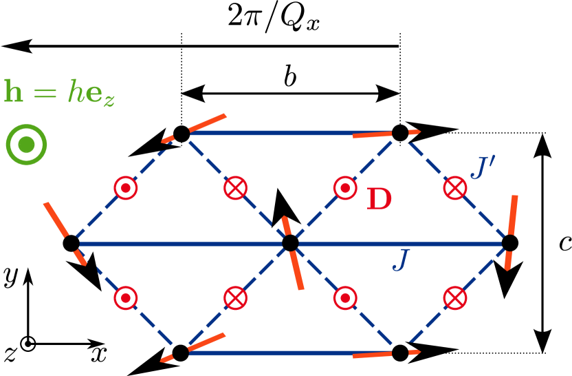
Figure 2: (Color online) Projection of the spin configuration in the cone state on the plane perpendicular to the magnetic field (the $x$-$y$ plane). The arrows represent the magnetic moments. The spiral state is characterized by the ordering vector $\bm{Q}=Q_{x}\hat{\bm{x}}$. Apart from the antiferromagnetic exchange interactions $J$ and $J^{\prime}$ there are also Dzyaloshinskii-Moriya interactions $\bm{D}=\pm D\hat{\bm{z}}$. Small circles with dots (crosses) denote vectors pointing out of (into) the $x$-$y$ plane.

The exchange couplings $J_{ij}=J(\bm{R}_{i}-\bm{R}_{j})$ connect nearest neighbors on the distorted triangular lattice with $J(\pm\bm{\delta}_{1})=J=0.374\,\text{meV}=4.34\,\text{K}$ and $J(\pm\bm{\delta}_{2})=J(\pm\bm{\delta}_{3})=J^{\prime}=0.128\,\text{meV}=1.49\,\text{K}$ where the three elementary direction vectors are

$$\bm{\delta}_{1} =b\hat{\bm{x}},\;\;\;\bm{\delta}_{2}=-\frac{b}{2}\hat{\bm{x}}+\frac{c}{2}\hat{\bm{y}},\;\;\;\bm{\delta}_{3}=-\frac{b}{2}\hat{\bm{x}}-\frac{c}{2}\hat{\bm{y}}.$$ (2)

Here $\hat{\bm{x}}$, $\hat{\bm{y}}$ and $\hat{\bm{z}}$ are unit vectors around the three Cartesian directions of our coordinate system. Due to the low symmetry of the crystal the spins are additionally coupled by an antisymmetric Dzyaloshinskii-Moriya interaction of the form $\bm{D}_{ij}=D_{ij}\hat{\bm{z}}$, where $D_{ij}=D(\bm{R}_{i}-\bm{R}_{j})$ is finite if $\bm{R}_{i}$ and $\bm{R}_{j}$ are nearest neighbors along the diagonal bonds.Starykh et al. (2010) The numerical value of the nearest-neighbor Dzyaloshinskii-Moriya coupling is $D(\pm\bm{\delta}_{2})=D(\pm\bm{\delta}_{3})=\mp D$ with $D=0.020\,\text{meV}=0.23\,\text{K}$.

The above spin model has continuous rotational symmetry with respect to rotations around the $z$ axis in spin space. As a consequence, one of the magnons is gapless, and the system does not exhibit any long-range order at any finite temperature.Mermin and Wagner (1966) If one nevertheless tries to calculate the magnetization at finite $T$ using spin-wave theory, one encounters an infrared divergence signaling the inconsistency of the assumption of finite magnetization. On the other hand, at vanishing temperature one should not expect any infrared divergencies because the fluctuations are not strong enough to destroy long-range magnetic order. In this work we will show that the spin-wave expansion for this model is nevertheless plagued by infrared divergencies which have to be resummed to all orders to obtain meaningful results. Similar singularities in the spin-wave expansion of the magnetic anisotropy energy of quantum antiferromagnets have been discussed some time ago by MaleyevMaleyev (2000) and by Syromyatnikov and Maleyev;Syromyatnikov and Maleyev (2001) however, these authors did not offer any strategy to resum these divergencies in order to obtain physical results.

The rest of this paper is organized as follows: In Sec. II we describe the spin-wave expansion in the cone state of Cs₂CuCl₄. To identify and isolate the infrared divergencies, we use a special parametrization of the spin-wave expansion in terms of Hermitian operators,Hasselmann and Kopietz (2006); Kreisel et al. (2007, 2008, 2011) which explicitly separates the longitudinal from the transverse spin fluctuations. In Sec. III we briefly recall some relevant results for the correlation functions of the interacting Bose gas and identify the corresponding parameters for the cone state of Cs₂CuCl₄. In Sec. IV we use the mapping of the bosonized spin-wave Hamiltonian in the cone state onto the interacting Bose gas to discuss the dynamic structure factor of Cs₂CuCl₄, which can be directly measured by means of neutron scattering. In particular, we show that in a magnetic field the dynamic structure factor exhibits scattering continua which are directly related to the well-known anomalous longitudinal fluctuations of the interacting Bose gas. Finally, in Sec. V we summarize our results and discuss ways to verify our theoretical prediction experimentally.

II Divergent spin-wave expansion in the cone state

In this section we shall set up the spin-wave expansion in the cone state of Cs₂CuCl₄ and identify the infrared divergent contributions. We first follow the conventional formulationKreisel et al. (2011) in terms of canonical boson operators introduced via the Holstein-Primakoff transformationHolstein and Primakoff (1940) and then show that an alternative parametrization of the $1/S$ expansion using Hermitian operatorsHasselmann and Kopietz (2006); Kreisel et al. (2007, 2008, 2011) allows us to isolate the infrared-divergent terms in a very efficient way.

II.1 Expansion in terms of canonical bosons

Before we set up the spin-wave expansion, we should determine the spin configuration in the classical ground state. Therefore we replace the spin operators by classical vectors of length $S=1/2$ pointing in the direction of the local magnetization.Veillette et al. (2005); Kreisel et al. (2011) For the triangular lattice antiferromagnet it has been shown that a finite magnetization in a spiral state is stable even in the presence of quantum fluctuations if the exchange parameters are in the rangeTrumper (1999); Note (1) $0.27J\lesssim J^{\prime}<2J$. Taking into account the Dzyaloshinskii-Moriya anisotropy with $D>0$, the classical ground-state energy,

$${\cal{H}}_{0}=\frac{S^{2}}{2}\sum_{ij}J^{\parallel}_{ij}-S\sum_{i}{\bm{h}}\cdot\hat{\bm{m}}_{i}\,,$$ (3)

is lowered compared to the situation without anisotropy, thus stabilizing the spiral state. Here we have defined

$$J_{ij}^{\parallel}=J_{ij}\hat{\bm{m}}_{i}\cdot\hat{\bm{m}}_{j}+{\bm{D}}_{ij}\cdot(\hat{\bm{m}}_{i}\times\hat{\bm{m}}_{j}).$$ (4)

In the presence of a magnetic field, the classical ground state is the so-called cone state, where the spins form a spiral that is tilted towards the direction of the field such that the magnetization $\hat{\bm{m}}_{i}$ on lattice point ${\bm{R}}_{i}$ is given byVeillette et al. (2005); Kreisel et al. (2011)

$$\hat{\bm{m}}_{i}=\sin\theta[\cos(\bm{Q}\cdot\bm{R}_{i})\hat{\bm{x}}+\sin(\bm{Q}\cdot\bm{R}_{i})\hat{\bm{y}}]+\cos\theta\hat{\bm{z}}.$$ (5)

This cone state is characterized by the opening angle $2\theta$ of the cone (see Fig. 1) and the wave vector $\bm{Q}$ of the spiral. Note that in Ref. [Kreisel et al., 2011] a different definition of the angle $\theta$ has been used, which amounts to the re-definition $\theta\rightarrow\pi-\theta$. The parameters $\theta$ and $\bm{Q}$ should be determined by minimizing classical ground state energy in Eq. (3). Anticipating that the spiral wave vector is of the formNote (2) $\bm{Q}=Q_{x}\hat{\bm{x}}$ as indicated in Fig. 2, it is easy to show that the classical ground-state energy is minimal if the angle $\theta$ is given by

$$\cos\theta=h/h_{c},$$ (6)

whereas the wave vector of the spiral obeys the equation,

$$\cos\left(\frac{Q_{x}b}{2}\right)=-\frac{J^{\prime}}{2J}-\frac{D}{2J}\cot\left(\frac{Q_{x}b}{2}\right)\,.$$ (7)

Here the critical magnetic field is given by

$$h_{c}=S(J^{D}_{0}-J^{D}_{\bm{Q}})=S(J_{0}-J_{\bm{Q}}+iD_{\bm{Q}}),$$ (8)

where we have introduced the Fourier transforms of the exchange integrals and the Dzyaloshinskii-Moriya interaction,

$$J_{\bm{k}}= 2J\cos(k_{x}b)+4J^{\prime}\cos\left(\frac{k_{x}b}{2}\right)\cos\left(\frac{k_{y}c}{2}\right),$$ (9)

$${{D}}_{\bm{k}}= -4iD\sin\left(\frac{k_{x}b}{2}\right)\cos\left(\frac{k_{y}c}{2}\right).$$ (10)

For later convenience, we have also introduced the real quantity,

$$J_{\bm{k}}^{D}=J_{\bm{k}}-iD_{\bm{k}}.$$ (11)

To set up the $1/S$ expansion, we project the spin operators at each lattice site $\bm{R}_{i}$ onto a local basis whose $z$ axis matches the direction of the classical ground state,

$$\bm{S}_{i}=S_{i}^{\parallel}\bm{\hat{m}}_{i}+S_{i}^{(1)}\bm{e}_{i}^{(1)}+S_{i}^{(2)}\bm{e}_{i}^{(2)}.$$ (12)

The convenient choice for the transverse basis vectors isKreisel et al. (2011)

$$\bm{e}^{(1)}_{i} =\sin(\bm{Q}\cdot\bm{R}_{i})\hat{\bm{x}}-\cos(\bm{Q}\cdot\bm{R}_{i})\hat{\bm{y}},$$ (13)

$$\bm{e}^{(2)}_{i} =\cos\theta[\cos(\bm{Q}\cdot\bm{R}_{i})\hat{\bm{x}}+\sin(\bm{Q}\cdot\bm{R}_{i})\hat{\bm{y}}]-\sin\theta\;\hat{\bm{z}}.$$ (14)

We then evaluate all scalar products and cross products of the basis vectors and express the components of the spin operators in terms of canonical boson operators $b_{i}$ and $b_{i}^{\dagger}$ using the Holstein-Primakoff transformation,Holstein and Primakoff (1940)

$$S_{i}^{\parallel} =S-n_{i},$$ (15a)

$$S_{i}^{+} =\sqrt{2S}\sqrt{1-\frac{n_{i}}{2S}}b_{i},$$ (15b)

$$S_{i}^{-} =\sqrt{2S}b^{\dagger}_{i}\sqrt{1-\frac{n_{i}}{2S}},$$ (15c)

where $n_{i}=b^{\dagger}_{i}b_{i}$. An expansion of the square roots generates the $1/S$ expansion and allows us to rewrite the Hamiltonian as

$${\cal{H}}={\cal{H}}_{0}+\sum_{n=2}^{\infty}{\cal{H}}_{n}\,,$$ (16)

with ${\cal{H}}_{n}\propto S^{2-n/2}$. The quadratic term describes noninteracting spin waves; in terms of the Fourier transforms of the boson operators,

$$b_{\bm{k}}=\frac{1}{\sqrt{N}}\sum_{i}e^{-i\bm{k}\cdot{\bm{R}}_{i}}b_{i},$$ (17)

we obtain

$${\cal{H}}_{2} =\sum_{\bm{k}}\Bigl{\{}A_{\bm{k}}b^{\dagger}_{\bm{k}}b_{\bm{k}}-\frac{B_{\bm{k}}}{2}\bigl{[}b^{\dagger}_{\bm{k}}b^{\dagger}_{-\bm{k}}+b_{-\bm{k}}b_{\bm{k}}\bigr{]}\Bigr{\}},$$ (18)

where $A_{\bm{k}}=A_{\bm{k}}^{+}+A_{\bm{k}}^{-}$ and

$$A^{+}_{\bm{k}} =B_{\bm{k}}-S\left[J^{D}_{\bm{Q}}-\frac{J^{D}_{\bm{Q}+\bm{k}}+J^{D}_{\bm{Q}-\bm{k}}}{2}\right]=A^{+}_{-\bm{k}},$$ (19a)

$$A^{-}_{\bm{k}} =S\cos{\theta}\frac{J^{D}_{\bm{Q}+\bm{k}}-J^{D}_{\bm{Q}-\bm{k}}}{2}=-A^{-}_{-\bm{k}},$$ (19b)

$$B_{\bm{k}} =\frac{S}{2}\sin^{2}\theta\left[J_{\bm{k}}-\frac{J^{D}_{\bm{Q}+\bm{k}}+J^{D}_{\bm{Q}-\bm{k}}}{2}\right]=B_{-\bm{k}}.$$ (19c)

The cubic term ${\cal{H}}_{3}$ describes the leading spin-wave interaction processes. In momentum space it can be written asKreisel et al. (2011)

$${\cal{H}}_{3} = \frac{1}{\sqrt{N}}\sum_{\bm{k}_{1}\bm{k}_{2}\bm{k}_{3}}\delta_{\bm{k}_{1}+\bm{k}_{2}+\bm{k}_{3},0}\Bigl{[}$$ (20)

$$\frac{1}{2!}\Gamma_{3}^{{b}^{\dagger}{b}^{\dagger}b}(\bm{k}_{1},\bm{k}_{2};\bm{k}_{3})b^{\dagger}_{-\bm{k}_{1}}b^{\dagger}_{-\bm{k}_{2}}b_{\bm{k}_{3}}$$

$$+ \frac{1}{2!}\Gamma_{3}^{{b}^{\dagger}bb}(\bm{k}_{1};\bm{k}_{2},\bm{k}_{3})b^{\dagger}_{-\bm{k}_{1}}b_{\bm{k}_{2}}b_{\bm{k}_{3}}\Bigr{]}.$$

The properly symmetrized cubic interaction vertices are

$$\Gamma_{3}^{{b}^{\dagger}{b}^{\dagger}b}(\bm{k}_{1},\bm{k}_{2};\bm{k}_{3}) =-\sin{\theta}\frac{\sqrt{2S}}{2i}\left[K_{-\bm{k}_{1}}+K_{-\bm{k}_{2}}\right],$$ (21a)

$$\Gamma_{3}^{{b}^{\dagger}bb}(\bm{k}_{1};\bm{k}_{2},\bm{k}_{3}) =\sin{\theta}\frac{\sqrt{2S}}{2i}\left[K_{\bm{k}_{2}}+K_{\bm{k}_{3}}\right],$$ (21b)

where

$$K_{\bm{k}}=\cos\theta\left[J_{\bm{k}}-\frac{J^{D}_{\bm{Q}+\bm{k}}+J^{D}_{\bm{Q}-\bm{k}}}{2}\right]-\frac{J^{D}_{\bm{Q}+\bm{k}}-J^{D}_{\bm{Q}-\bm{k}}}{2}.$$ (22)

Finally, the quartic part ${\cal{H}}_{4}$ of the interaction can be written as

$${\cal{H}}_{4} =\frac{1}{N}\sum_{\bm{k}_{1}\bm{k}_{2}\bm{k}_{3}\bm{k}_{4}}\delta_{\bm{k}_{1}+\bm{k}_{2}+\bm{k}_{3}+\bm{k}_{4},0}\Bigl{[}$$

$$\frac{1}{(2!)^{2}}\Gamma_{4}^{{b}^{\dagger}{b}^{\dagger}bb}(\bm{k}_{1},\bm{k}_{2};\bm{k}_{3},\bm{k}_{4})b^{\dagger}_{-\bm{k}_{1}}b^{\dagger}_{-\bm{k}_{2}}b_{\bm{k}_{3}}b_{\bm{k}_{4}}$$

$$+\frac{1}{3!}\Gamma_{4}^{{b}^{\dagger}bbb}(\bm{k}_{1};\bm{k}_{2},\bm{k}_{3},\bm{k}_{4})b^{\dagger}_{-\bm{k}_{1}}b_{\bm{k}_{2}}b_{\bm{k}_{3}}b_{\bm{k}_{4}}$$

$$+\frac{1}{3!}[\Gamma_{4}^{{b}^{\dagger}bbb}(\bm{k}_{1};\bm{k}_{2},\bm{k}_{3},\bm{k}_{4})]^{*}b^{\dagger}_{-\bm{k}_{4}}b^{\dagger}_{-\bm{k}_{3}}b^{\dagger}_{-\bm{k}_{2}}b_{\bm{k}_{1}}\Bigr{]}.$$ (23)

The vertices are

$$\Gamma_{4}^{{b}^{\dagger}{b}^{\dagger}bb}(\bm{k}_{1},\bm{k}_{2};\bm{k}_{3},\bm{k}_{4}) =-\frac{1}{8}\sum_{i=1}^{4}(J_{\bm{k}_{i}}^{\pm}+J_{-\bm{k}_{i}}^{\mp})$$

$$+\frac{1}{2}(J_{\bm{k}_{1}-\bm{k}_{3}}^{\parallel}+J_{\bm{k}_{2}-\bm{k}_{3}}^{\parallel}+J_{\bm{k}_{1}-\bm{k}_{4}}^{\parallel}+J_{\bm{k}_{2}-\bm{k}_{4}}^{\parallel}),$$ (24a)

$$\Gamma_{4}^{{b}^{\dagger}bbb}(\bm{k}_{1};\bm{k}_{2},\bm{k}_{3},\bm{k}_{4}) =-\frac{1}{4}(J_{\bm{k}_{2}}^{++}+J_{\bm{k}_{3}}^{++}+J_{\bm{k}_{4}}^{++}),$$ (24b)

with

$$J^{\parallel}_{\bm{k}} = \cos^{2}\theta J_{\bm{k}}+\sin^{2}{\theta}\frac{J^{D}_{\bm{Q}+\bm{k}}+J^{D}_{\bm{Q}-\bm{k}}}{2},$$ (25a)

$$J^{+-}_{\bm{k}} = J^{-+}_{-\bm{k}}=\sin^{2}{\theta}J_{\bm{k}}+(1+\cos^{2}{\theta})\frac{J^{D}_{\bm{Q}+\bm{k}}+J^{D}_{\bm{Q}-\bm{k}}}{2}$$ (25b)

$$\hskip 36.98866pt+\cos{\theta}\left[J^{D}_{\bm{Q}+\bm{k}}-J^{D}_{\bm{Q}-\bm{k}}\right],$$

$$J^{++}_{\bm{k}} = J^{--}_{\bm{k}}=-\sin^{2}{\theta}\left[J_{\bm{k}}-\frac{J^{D}_{\bm{Q}+\bm{k}}+J^{D}_{\bm{Q}-\bm{k}}}{2}\right].$$ (25c)

To obtain the magnon dispersion of our model, we diagonalize ${\cal{H}}_{2}$ in Eq. (18) by means of a Bogoliubov transformation and obtainKreisel et al. (2011)

$${\cal{H}}_{2}=\sum_{\bm{k}}\left[E_{\bm{k}}\beta^{\dagger}_{\bm{k}}\beta_{\bm{k}}+\frac{\epsilon_{\bm{k}}-A^{+}_{\bm{k}}}{2}\right]\,,$$ (26)

where $\beta^{\dagger}_{\bm{k}}$ and $\beta_{\bm{k}}$ are again canonical boson operators and the magnon dispersion is

$$E_{\bm{k}}=\epsilon_{\bm{k}}+A^{-}_{\bm{k}},$$ (27)

with

$$\epsilon_{\bm{k}}=\sqrt{(A^{+}_{\bm{k}})^{2}-B_{\bm{k}}^{2}}\,.$$ (28)

Using the fact that for small wave vectors the antisymmetric contribution is negligible,

$$A^{-}_{\bm{k}}={\mathcal{O}}(\bm{k}^{3}),$$ (29)

it is easy to show that at long wavelengths the magnons have a linear dispersion,

$$E_{\bm{k}}=\epsilon_{\bm{k}}+{\mathcal{O}}(\bm{k}^{3})=v({\hat{\bm{k}}})|\bm{k}|+{\mathcal{O}}(\bm{k}^{3}),$$ (30)

with direction-dependent magnon velocity

$$v({\hat{\bm{k}}})=\sqrt{v_{x}^{2}\hat{k}_{x}^{2}+v_{y}^{2}\hat{k}_{y}^{2}},$$ (31)

where $\hat{\bm{k}}=\bm{k}/|\bm{k}|$. The Cartesian components of the squares of the magnon velocity are explicitly

$$v_{x}^{2} =Sh_{c}b^{2}\sin^{2}\theta\biggl{[}-J\cos(Q_{x}b)-\frac{J^{\prime}}{2}\cos\Bigl{(}\frac{Q_{x}b}{2}\Bigr{)}$$

$$\hskip 56.9055pt+\frac{D}{2}\cos\Bigl{(}\frac{Q_{x}b}{2}\Bigr{)}\biggr{]},$$ (32)

$$v_{y}^{2} =Sh_{c}c^{2}\sin^{2}\theta\biggl{[}-\frac{J^{\prime}}{2}\cos\Bigl{(}\frac{Q_{x}b}{2}\Bigr{)}+\frac{D}{2}\cos\Bigl{(}\frac{Q_{x}b}{2}\Bigr{)}\biggr{]}.$$

(33)

A graph of the velocity components $v_{x}$ and $v_{y}$ as a function of the magnetic field is shown in Fig. 3.

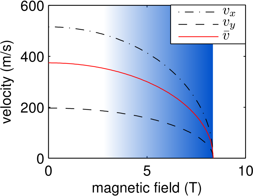
Figure 3: (Color online) Plot of the magnon velocities $v_{x}$ (dashed line) and $v_{y}$ (dashed-dotted line) defined in Eqs. (32) and(33) for the parameters relevant for Cs₂CuCl₄. The solid (red) line represents the angular averaged velocity defined in Eq. (76). The shaded (blue) area is the regime close to the saturation field where our mapping to the Bose gas is quantitatively accurate.

An important observation is that the cubic interaction vertices in Eqs. (21a) and (21b) have finite limits when all wave-vectors vanish. Using the fact that

$$K_{0}=\cos\theta(J_{0}-J_{\bm{Q}}^{D})=\cos{\theta}\frac{h_{c}}{S}=\frac{h}{S},$$ (34)

we obtain

$$\Gamma_{3}^{{b}^{\dagger}{b}^{\dagger}b}(0,0;0) =-\Gamma_{3}^{{b}^{\dagger}bb}(0;0,0)$$

$$=2i\sin\theta\cos{\theta}\frac{h_{c}}{\sqrt{2S}}.$$ (35)

In the next section we will show that the linear magnon dispersion in combination with finite cubic interaction vertices imply that the magnon self-energy generated by the spin-wave interactions is infrared divergent.

II.2 Expansion in terms of Hermitian field operators

To calculate corrections to linear spin-wave theory in powers of the formal small parameter $1/S$, we now use conventional many-body methods for bosons. We find that the perturbation series for the magnon self-energy contains already at order $1/S$ some infrared-divergent terms. Unfortunately, in the conventional formulation of the spin-wave expansion using the Bogoliubov bosons $\beta_{\bm{k}}$ and $\beta_{\bm{k}}^{\dagger}$, which diagonalize the quadratic Hamiltonian the calculations become rather cumbersome because the interactions in this basis contain the singular coefficients of the Bogoliubov transformation which is necessary to bring the quadratic Hamiltonian (18) to the diagonal form (26). One can avoid this problem by directly generating the perturbation expansion in terms of the Holstein-Primakoff bosons,Maleyev (2000) but then one has to deal with anomalous propagators and off-diagonal magnon self-energies. Fortunately, there is an alternative parametrization of the spin-wave expansion using Hermitian operatorsHasselmann and Kopietz (2006); Kreisel et al. (2007, 2008, 2011) which greatly facilitates the identification of the singular terms in the spin-wave expansion around the cone state of Cs₂CuCl₄. In this approach, one expresses the Holstein-Primakoff bosons in terms of Hermitian operators $\Pi_{\bm{k}}$ and $\Phi_{\bm{k}}$ by setting

$$b_{\bm{k}}=\frac{1}{\sqrt{2}}[\Phi_{\bm{k}}+i\Pi_{\bm{k}}]\;,\;\;\;b_{\bm{k}}^{\dagger}=\frac{1}{\sqrt{2}}[\Phi_{-\bm{k}}-i\Pi_{-\bm{k}}]\;.$$ (36)

By demanding that $[\Phi_{\bm{k}},\Pi_{\bm{k}}]=i\delta_{\bm{k},-\bm{k}^{\prime}}$ and that all other commutators vanish, it is easy to see that the canonical commutation relations $[b_{\bm{k}},b^{\dagger}_{\bm{k}^{\prime}}]=\delta_{\bm{k},\bm{k}^{\prime}}$ are satisfied. Then we obtain from Eq. (18) for the quadratic part of the spin-wave Hamiltonian,

$${\cal{H}}_{2} = \frac{1}{2}\sum_{\bm{k}}\Bigl{[}\Delta_{\bm{k}}{\Pi}_{-\bm{k}}{\Pi}_{\bm{k}}+\frac{\epsilon_{\bm{k}}^{2}}{\Delta_{\bm{k}}}{\Phi}_{-\bm{k}}{\Phi}_{\bm{k}}-A^{+}_{\bm{k}}$$ (37)

$$\hskip 19.91692pt+iA^{-}_{\bm{k}}({\Phi}_{-\bm{k}}{\Pi}_{\bm{k}}-{\Pi}_{-\bm{k}}{\Phi}_{\bm{k}})\Bigr{]},$$

where $\epsilon_{\bm{k}}$ and $A_{\bm{k}}^{-}$ are defined in Eq. (28) and (19b), and

$$\Delta_{\bm{k}}=A_{\bm{k}}^{+}+B_{\bm{k}}.$$ (38)

Using Eqs. (19a) and (19c) we find that for $\bm{k}\rightarrow 0$ the energy scale $\Delta_{\bm{k}}$ approaches a finite limit,

$$\Delta_{0}=h_{c}\sin^{2}\theta=h_{c}\left[1-\frac{h^{2}}{h_{c}^{2}}\right],$$ (39)

such that the operator $\Phi_{\bm{k}}$ is associated with the transverse fluctuations and $\Pi_{\bm{k}}$ is associated with the longitudinal fluctuations as it will become more clear in Sec. III. The cubic part ${\cal{H}}_{3}$ of our spin-wave Hamiltonian in Eq. (20) can be written as

$${\cal{H}}_{3} = \frac{1}{\sqrt{N}}\sum_{\bm{k}_{1}\bm{k}_{2}\bm{k}_{3}}\delta_{\bm{k}_{1}+\bm{k}_{2}+\bm{k}_{3},0}\Bigl{[}$$ (40)

$$\frac{1}{3!}\Gamma^{\Phi\Phi\Phi}(\bm{k}_{1},\bm{k}_{2},\bm{k}_{3}){\Phi}_{\bm{k}_{1}}{\Phi}_{\bm{k}_{2}}{\Phi}_{\bm{k}_{3}}$$

$$+ \frac{1}{3!}\Gamma^{\Pi\Pi\Pi}(\bm{k}_{1},\bm{k}_{2},\bm{k}_{3}){\Pi}_{\bm{k}_{1}}{\Pi}_{\bm{k}_{2}}{\Pi}_{\bm{k}_{3}}$$

$$+ \frac{1}{2!}\Gamma^{\Phi\Phi\Pi}(\bm{k}_{1},\bm{k}_{2};\bm{k}_{3}){\Phi}_{\bm{k}_{1}}{\Phi}_{\bm{k}_{2}}{\Pi}_{\bm{k}_{3}}$$

$$+ \frac{1}{2!}\Gamma^{\Pi\Pi\Phi}(\bm{k}_{1},\bm{k}_{2};\bm{k}_{3}){\Pi}_{\bm{k}_{1}}{\Pi}_{\bm{k}_{2}}{\Phi}_{\bm{k}_{3}}\Bigr{]}.$$

The properly symmetrized vertices are

$$\Gamma^{\Phi\Phi\Phi}(\bm{k}_{1},\bm{k}_{2},\bm{k}_{3})= -i\left[V_{-}(\bm{k}_{1})+V_{-}(\bm{k}_{2})+V_{-}(\bm{k}_{3})\right]\,,$$ (41a)

$$\Gamma^{\Pi\Pi\Pi}(\bm{k}_{1},\bm{k}_{2},\bm{k}_{3})= V_{+}(\bm{k}_{1})+V_{+}(\bm{k}_{2})+V_{+}(\bm{k}_{3}),$$ (41b)

$$\Gamma^{\Pi\Pi\Phi}(\bm{k}_{1},\bm{k}_{2};\bm{k}_{3})= -iV_{-}(\bm{k}_{3})\,,$$ (41c)

$$\Gamma^{\Phi\Phi\Pi}(\bm{k}_{1},\bm{k}_{2};\bm{k}_{3})= V_{+}(\bm{k}_{3})\,,$$ (41d)

where

$$V_{\pm}(\bm{k})=\sqrt{S}\sin\theta\frac{K_{\bm{k}}\pm K_{-\bm{k}}}{2}\,,$$ (42)

and $K_{\bm{k}}$ is defined in Eq. (22). For small wave vectors we find

$$V_{+}(\bm{k}) =\sin\theta\cos\theta\frac{h_{c}}{\sqrt{S}}+{\cal{O}}(\bm{k}^{2}),$$ (43)

$$V_{-}(\bm{k}) ={\cal{O}}(\bm{k}^{3}).$$ (44)

In deriving Eq. (40) we have ignored terms linear in the field operators which are related to the specific ordering of the operators in this equation. These terms do not affect the infrared divergencies discussed below.

Let us now attempt to calculate the effect of the cubic part ${\cal{H}}_{3}$ of the spin-wave interactions on the magnon propagators. Therefore it is convenient to formulate the perturbation theory in terms of an imaginary-time functional integral. Formally, we simply have to replace the field operators $\Phi_{\bm{k}}$ and $\Pi_{\bm{k}}$ by Hermitian fields $\Phi_{\bm{k}}(\tau)$ and $\Pi_{\bm{k}}(\tau)$ depending on imaginary time $\tau$. We denote the corresponding Fourier components in frequency space by $\Phi_{K}$ and $\Pi_{K}$ where $K=(\bm{k},i\omega)$ is the collective label for the momentum $\bm{k}$ and the bosonic Matsubara frequency $i\omega$. The quadratic part ${\cal{H}}_{2}$ of our spin-wave Hamiltonian given in Eq. (18) corresponds then to the following Gaussian Euclidean action,

$$S_{2}[{\Phi},{\Pi}] = \frac{\beta}{2}\sum_{K}\Bigl{[}\Delta_{\bm{k}}{\Pi}_{-K}{\Pi}_{K}+\frac{\epsilon_{\bm{k}}^{2}}{\Delta_{\bm{k}}}{\Phi}_{-K}{\Phi}_{K}$$ (45)

$$+(\omega+iA_{\bm{k}}^{-})({\Phi}_{-K}{\Pi}_{K}-{\Pi}_{-K}{\Phi}_{K})\Bigr{]}.\hskip 19.91692pt$$

From the Gaussian action (45) we obtain the free propagators,

$$\beta\langle\Phi_{K}\Phi_{K^{\prime}}\rangle = \delta_{\bm{k},-\bm{k}^{\prime}}\delta_{\omega,-\omega^{\prime}}G_{0}^{\Phi\Phi}(K),$$ (46a)

$$\beta\langle\Pi_{K}\Pi_{K^{\prime}}\rangle = \delta_{\bm{k},-\bm{k}^{\prime}}\delta_{\omega,-\omega^{\prime}}G_{0}^{\Pi\Pi}(K),$$ (46b)

$$\beta\langle\Phi_{K}\Pi_{K^{\prime}}\rangle = \delta_{\bm{k},-\bm{k}^{\prime}}\delta_{\omega,-\omega^{\prime}}G_{0}^{\Phi\Pi}(K),$$ (46c)

with

$$G_{0}^{\Phi\Phi}(K) = \frac{\Delta_{\bm{k}}}{\epsilon_{\bm{k}}^{2}+\left[\omega+iA_{\bm{k}}^{-}\right]^{2}}\approx\frac{\Delta_{0}}{\epsilon_{\bm{k}}^{2}+\omega^{2}},$$ (47a)

$$G_{0}^{\Pi\Pi}(K) = \frac{\epsilon_{\bm{k}}^{2}/\Delta_{\bm{k}}}{\epsilon_{\bm{k}}^{2}+\left[\omega+iA_{\bm{k}}^{-}\right]^{2}}\approx\frac{\epsilon_{\bm{k}}^{2}/\Delta_{0}}{\epsilon_{\bm{k}}^{2}+\omega^{2}},$$ (47b)

$$G_{0}^{\Phi\Pi}(K) = \frac{\omega+iA_{\bm{k}}^{-}}{\epsilon_{\bm{k}}^{2}+\left[\omega+iA_{\bm{k}}^{-}\right]^{2}}\approx\frac{\omega}{\epsilon_{\bm{k}}^{2}+\omega^{2}}.$$ (47c)

We have also given the leading approximations for small $\bm{k}$ where $\epsilon_{\bm{k}}\approx v(\hat{\bm{k}})|\bm{k}|$. In the presence of interactions the coefficients in Eq. (45) acquire self-energy corrections, so that the quadratic part of the true effective action is of the form

$$\Gamma_{2}[{\Phi},{\Pi}] = \frac{\beta}{2}\sum_{K}\Bigl{\{}\left[\Delta_{\bm{k}}+\Sigma^{\Pi\Pi}(K)\right]{\Pi}_{-K}{\Pi}_{K}$$

$$+ \left[\epsilon_{\bm{k}}^{2}/\Delta_{\bm{k}}+\Sigma^{\Phi\Phi}(K)\right]{\Phi}_{-K}{\Phi}_{K}$$

$$+ \left[\omega+iA_{\bm{k}}^{-}+\Sigma^{\Phi\Pi}(K)\right]({\Phi}_{-K}{\Pi}_{K}-{\Pi}_{-K}{\Phi}_{K})\Bigr{\}}.$$

The corresponding propagators are

$$G^{\Phi\Phi}(K) = \frac{\Delta_{\bm{k}}+\Sigma^{\Pi\Pi}(K)}{D(K)},$$ (49a)

$$G^{\Pi\Pi}(K) = \frac{\epsilon_{\bm{k}}^{2}/\Delta_{\bm{k}}+\Sigma^{\Phi\Phi}(K)}{D(K)},$$ (49b)

$$G^{\Phi\Pi}(K) = \frac{\omega+iA_{\bm{k}}^{-}+\Sigma^{\Phi\Pi}(K)}{D(K)},$$ (49c)

where the determinant is given by

$$D(K) = \left[\Delta_{\bm{k}}+\Sigma^{\Pi\Pi}(K)\right]\left[\epsilon_{\bm{k}}^{2}/\Delta_{\bm{k}}+\Sigma^{\Phi\Phi}(K)\right]$$ (50)

$$+ \left[\omega+iA_{\bm{k}}^{-}+\Sigma^{\Phi\Pi}(K)\right]^{2}.$$

The crucial advantage of the above Hermitian field parametrization is that it allows us to isolate in a very simple way the infrared-divergent contributions to the self-energies arising in second order perturbation theory in the cubic vertices. It turns out that only terms involving the vertex $\Gamma^{\Phi\Phi\Pi}(\bm{k}_{1},\bm{k}_{2};\bm{k}_{3})=V_{+}(\bm{k}_{3})$ give rise to infrared-divergent terms. Moreover, since we are only interested in the infrared divergencies, we may approximate

$$\Gamma^{\Phi\Phi\Pi}(\bm{k}_{1},\bm{k}_{2};\bm{k}_{3})\approx V_{+}(0)=\sin\theta\cos\theta\frac{h_{c}}{\sqrt{S}}.$$ (51)

The Feynman diagrams giving the leading singular contributions to the self-energies are shown in Fig. 4. For small wave vectors these diagrams correspond to the following self-energies,

$$\Sigma^{\Phi\Phi}(K) \approx -\frac{|V_{+}(0)|^{2}}{\beta N}\sum_{K^{\prime}}\bigl{[}G_{0}^{\Phi\Phi}(K^{\prime})G_{0}^{\Pi\Pi}(K-K^{\prime})$$ (52a)

$$\hskip 34.1433pt+G_{0}^{\Phi\Pi}(K^{\prime})G_{0}^{\Pi\Phi}(K-K^{\prime})\bigr{]},$$

$$\Sigma^{\Pi\Pi}(K) \approx -\frac{|V_{+}(0)|^{2}}{2\beta N}\sum_{K^{\prime}}G_{0}^{\Phi\Phi}(K^{\prime})G_{0}^{\Phi\Phi}(K-K^{\prime}),$$

$$\Sigma^{\Phi\Pi}(K) \approx -\frac{|V_{+}(0)|^{2}}{\beta N}\sum_{K^{\prime}}G_{0}^{\Phi\Phi}(K^{\prime})G_{0}^{\Pi\Phi}(K-K^{\prime}).$$

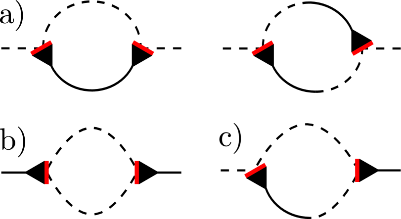
Figure 4: (Color online) Graphical representation of the singular contributions to the magnon self-energies. The diagrams (a) in the first line give the singular contribution to $\Sigma^{\Phi\Phi}(K)$ in Eq. (52a). Diagrams (b) and (c) represent the singular contributions to $\Sigma^{\Pi\Pi}(K)$ and $\Sigma^{\Phi\Pi}(K)$ given in Eqs. (LABEL:eq:sigma2) and (LABEL:eq:sigma3). Solid lines are propagators $G^{\Phi\Phi}$, dashed lines are propagators $G^{\Pi\Pi}$, and the solid-dashed lines represent the off-diagonal propagators $G^{\Phi\Pi}$ and $G^{\Pi\Phi}$. The three-legged vertex $\Gamma^{\Phi\Phi\Pi}$ is represented by a black triangle with a red (gray) bar reflecting the symmetry with respect to the permutation of the external fields.

Using the long-wavelength approximations of the Gaussian propagators given in Eqs. (47a)-(47c), we obtain for small frequencies and momenta to leading order,

$$\Sigma^{\Phi\Phi}(K) \approx \alpha\omega^{2}/\Delta_{0},$$ (53a)

$$\Sigma^{\Pi\Pi}(K) \approx -2\alpha\Delta_{0},$$ (53b)

$$\Sigma^{\Phi\Pi}(K) \approx -2\alpha\omega,$$ (53c)

where the dimensionless factor $\alpha$ is given by

$$\alpha=\frac{\Delta_{0}|V_{+}(0)|^{2}}{16N}\sum_{\bm{k}}\frac{1}{\epsilon_{\bm{k}}^{3}}=\frac{\cos\theta\sin^{3}\theta}{16SN}\sum_{\bm{k}}\frac{h_{c}^{3}}{\epsilon_{\bm{k}}^{3}}.$$ (54)

Keeping in mind that for small wavevectors $\epsilon_{\bm{k}}\propto|\bm{k}|$, it is obvious that for $D\leq 3$ the factor $\alpha$ is infrared divergent. Note further that the first-order contribution generated by the quartic part of the Hamiltonian as given in Eq. (23) is on the same order in $1/S$ as the terms just discussed; however, the former contributions are all finite and give rise to finite renormalizations of the bare parameters, such as the spin-wave velocities $v_{x}$ and $v_{y}$. We conclude that the leading $1/S$ correction to linear spin-wave theory in the cone state of Cs₂CuCl₄ diverges even at zero temperature.

III Correlation functions of interacting bosons in two dimensions

In this section we show that the infrared singularities in the $1/S$ expansion around the cone state of Cs₂CuCl₄ are actually familiar from the theory of the condensed phase of the interacting Bose gas. The linear spin-wave theory corresponds in the Bose gas to Bogoliubov’s mean-field theory for the condensed phase, leading to the well-known linear phonon spectrum. But if one tries to calculate fluctuation corrections to mean-field theory one encounters in dimensions $D\leq 3$ infrared divergencies which arise from the coupling between longitudinal and transverse fluctuations in the condensed phase.Shi and Griffin (1998); Andersen (2004); Sinner et al. (2009); *Sinner10; Dupuis (2011) To leading order in perturbation theory, this coupling is described by a triangular vertex similar to $\Gamma^{\Phi\Phi\Pi}(\bm{k}_{1},\bm{k}_{2};\bm{k}_{3})$ given in Eq. (41d) where the field $\Pi$ describes longitudinal fluctuations of the complex order parameter, whereas the field $\Phi$ describes transverse fluctuations perpendicular to the direction of the order parameter. The reason why the $1/S$-expansion of many other quantum magnets is not plagued by similar singularities is that usually the triangular vertex vanishes at long wavelengths due to spin conservation or is identically zero by symmetry. Conversely, if the magnon spectrum is gapless and the usual $1/S$ expansion around the classical ground state generates a triangular vertex which reduces to a constant at long wavelengths, then the leading $1/S$ correction to linear spin-wave theory is singular in dimensions $D\leq 3$. Similar singularities appear also in the interaction corrections to the spin-wave gap in anisotropic square lattice antiferromagnets.Maleyev (2000); Syromyatnikov and Maleyev (2001) In this case the magnon spectrum is not gapless, but the triangular vertices in the $1/S$ expansion are finite, leading to a singular renormalization of the spin-wave gap.

To obtain physically meaningful results, the singularities encountered in the $1/S$ expansion around the cone state should be cured by some nonperturbative procedure which takes the singular corrections to all orders in the $1/S$ expansion into account. Although within the conventional formulation of the $1/S$ expansion this cannot be performed, we can achieve this by using known nonperturbative results for the interacting Bose gasWeichman (1988); Giorgini et al. (1992); Castellani et al. (1997); Pistolesi et al. (2004). Let us therefore summarize in this section the relevant results for the Bose gas. In Sec. IV we will then apply these results to our model for Cs₂CuCl₄.

We consider a system of interacting bosons confined to a volume $V$ with Hamiltonian,

$$\tilde{\cal{H}}=\sum_{\bm{k}}\frac{\bm{k}^{2}}{2m}b^{\dagger}_{\bm{k}}b_{\bm{k}}+\frac{1}{2V}\sum_{\bm{k}\bm{k}^{\prime}\bm{q}}u_{\bm{q}}b^{\dagger}_{\bm{k}+\bm{q}}b^{\dagger}_{\bm{k}^{\prime}-\bm{q}}b_{\bm{k}^{\prime}}b_{\bm{k}},$$ (55)

where the Fourier transform $u_{\bm{q}}$ of the interaction has a finite limit for vanishing momentum transfer $\bm{q}$. In the condensed phase the single particle state with $\bm{k}=0$ is macroscopically occupied, so that the expectation value $\langle b_{\bm{k}=0}\rangle$ is proportional to $\sqrt{V}$. We take this macroscopic occupation of the $\bm{k}=0$ state into account via the usual Bogoliubov shift. In order to emphasize the analogy with the spin-wave approach for Cs₂CuCl₄ outlined in Sec. II, it is convenient to assume that the expectation value of $b_{\bm{k}=0}$ is purely imaginary so that we should set

$$b_{0}=i\sqrt{N_{0}}+\delta b_{0},$$ (56)

where $N_{0}$ is the number of condensed bosons. Substituting this into Eq. (55) and subtracting the chemical potential term $\mu{\cal{N}}=\mu\sum_{\bm{k}}b^{\dagger}_{\bm{k}}b_{\bm{k}}$, we obtain

$$\tilde{\cal{H}}-\mu{\cal{N}}=\left(\frac{\rho_{0}u_{0}}{2}-\mu\right)N_{0}+\tilde{\cal{H}}_{1}+\tilde{\cal{H}}_{2}+\tilde{\cal{H}}_{3}+\tilde{\cal{H}}_{4},$$ (57)

where

$${\cal{\tilde{H}}}_{1} = i\sqrt{N_{0}}(\rho_{0}u_{0}-\mu)(\delta b_{0}^{\dagger}-\delta b_{0}),$$ (58)

$${\cal{\tilde{H}}}_{2} = \sum_{\bm{k}}\Bigl{\{}\Bigl{[}\frac{{\bm{k}}^{2}}{2m}+\rho_{0}u_{\bm{k}}+\rho_{0}u_{0}-\mu\Bigr{]}b^{\dagger}_{\bm{k}}b_{\bm{k}}$$ (59)

$$\hskip 19.91692pt-\frac{\rho_{0}u_{\bm{k}}}{2}\bigl{[}b^{\dagger}_{\bm{k}}b^{\dagger}_{-\bm{k}}+b_{-\bm{k}}b_{\bm{k}}\bigr{]}\Bigr{\}},$$

$${\cal{\tilde{H}}}_{3} = \frac{1}{\sqrt{N_{0}}}\sum_{\bm{k}_{1}\bm{k}_{2}\bm{k}_{3}}\delta_{\bm{k}_{1}+\bm{k}_{2}+\bm{k}_{3},0}\Bigl{[}$$ (60)

$$\frac{i\rho_{0}}{2!}(u_{\bm{k}_{1}}+u_{\bm{k}_{2}})b^{\dagger}_{-\bm{k}_{1}}b^{\dagger}_{-\bm{k}_{2}}b_{\bm{k}_{3}}$$

$$- \frac{i\rho_{0}}{2!}(u_{\bm{k}_{2}}+u_{\bm{k}_{3}})b^{\dagger}_{-\bm{k}_{1}}b_{\bm{k}_{2}}b_{\bm{k}_{3}}\Bigr{]}.$$

Here $\rho_{0}=N_{0}/V$ is the condensate density. In ${\cal{\tilde{H}}}_{2}$ and ${\cal{\tilde{H}}}_{3}$ it is understood that we should substitute $b_{\bm{k}=0}\rightarrow\delta b_{0}$. With this convention ${\cal{\tilde{H}}}_{4}$ has the same form as the interaction in our original Hamiltonian (55). As in the spin-wave approach, we demand that the linear term ${\cal{\tilde{H}}}_{1}$ vanishes identically, implying the Hugenholtz-Pines identity,Shi and Griffin (1998); Andersen (2004)

$$\rho_{0}u_{0}=\mu,$$ (61)

which fixes the condensate density $\rho_{0}=\mu/u_{0}$ as a function of the chemical potential and the interaction. The quadratic term then simplifies to

$${\cal{\tilde{H}}}_{2} =\sum_{\bm{k}}\Bigl{\{}\Bigl{[}\frac{{\bm{k}}^{2}}{2m}+\rho_{0}u_{\bm{k}}\Bigr{]}b^{\dagger}_{\bm{k}}b_{\bm{k}}-\frac{\rho_{0}u_{\bm{k}}}{2}\bigl{[}b^{\dagger}_{\bm{k}}b^{\dagger}_{-\bm{k}}+b_{-\bm{k}}b_{\bm{k}}\bigr{]}\Bigr{\}}.$$ (62)

After diagonalization via a Bogoliubov transformation we obtain

$${\cal{\tilde{H}}}_{2}=\sum_{\bm{k}}\left[{\epsilon}_{\bm{k}}\beta^{\dagger}_{\bm{k}}\beta_{\bm{k}}+\frac{1}{2}\left({\epsilon}_{\bm{k}}-\frac{{\bm{k}}^{2}}{2m}-\rho_{0}u_{\bm{k}}\right)\right]\,,$$ (63)

where $\beta^{\dagger}_{\bm{k}}$ and $\beta_{\bm{k}}$ are again canonical boson operators and the boson dispersion is

$${\epsilon}_{\bm{k}} = \sqrt{\Bigl{(}\frac{{\bm{k}}^{2}}{2m}+\rho_{0}u_{\bm{k}}\Bigr{)}^{2}-(\rho_{0}u_{\bm{k}})^{2}}$$ (64)

$$= \sqrt{\frac{\bm{k}^{2}}{m}\rho_{0}u_{\bm{k}}+\left(\frac{\bm{k}^{2}}{2m}\right)^{2}}.$$

For small wave vectors we obtain the well-known linear phonon dispersion,

$$\epsilon_{\bm{k}}=c_{0}|\bm{k}|+{\cal{O}}(\bm{k}^{3}),$$ (65)

with phonon velocity

$$c_{0}=\sqrt{\frac{\rho_{0}u_{0}}{m}}=\sqrt{\frac{\mu}{m}}.$$ (66)

To facilitate the identification of the infrared divergent terms in perturbation theory, we now introduce again Hermitian field operators as in Eq. (36). Note that with our phase convention the $\Pi$ field describes longitudinal fluctuations in the direction of the order parameter whereas the $\Phi$ field is associated with transverse fluctuations. Substituting the transformation (36) into Eq. (62) we obtain for the quadratic part of the Hamiltonian,

$${\cal{\tilde{H}}}_{2} = \frac{1}{2}\sum_{\bm{k}}\Bigl{[}\Bigl{(}2\rho_{0}u_{\bm{k}}+\frac{\bm{k}^{2}}{2m}\Bigr{)}{\Pi}_{-\bm{k}}{\Pi}_{\bm{k}}+\frac{\bm{k}^{2}}{2m}{\Phi}_{-\bm{k}}{\Phi}_{\bm{k}}$$

$$\hskip 28.45274pt-\Bigl{(}\rho_{0}u_{\bm{k}}+\frac{\bm{k}^{2}}{2m}\Bigr{)}\Bigr{]}$$

$$= \frac{1}{2}\sum_{\bm{k}}\Bigl{[}\Delta_{\bm{k}}{\Pi}_{-\bm{k}}{\Pi}_{\bm{k}}+\frac{\epsilon_{\bm{k}}^{2}}{\Delta_{\bm{k}}}{\Phi}_{-\bm{k}}{\Phi}_{\bm{k}}-\Bigl{(}\rho_{0}u_{\bm{k}}+\frac{\bm{k}^{2}}{2m}\Bigr{)}\Bigr{]},$$

where in this section,

$$\Delta_{\bm{k}}=2\rho_{0}u_{\bm{k}}+\frac{\bm{k}^{2}}{2m}.$$ (68)

Our notation emphasizes the formal similarity between Eqs. (LABEL:eq:hbos2) and (37); the additional term in Eq. (37) involving the antisymmetric factor $A_{\bm{k}}^{-}$ complicates the expression, but does not change the final result because of Eq. (29). Ignoring again commutator terms involving a single power of the fields, the leading interaction part ${\cal{\tilde{H}}}_{3}$ of our boson Hamiltonian can be written as

$$\tilde{{\cal{H}}}_{3} = \frac{1}{\sqrt{N_{0}}}\sum_{\bm{k}_{1}\bm{k}_{2}\bm{k}_{3}}\delta_{\bm{k}_{1}+\bm{k}_{2}+\bm{k}_{3},0}\Bigl{[}$$ (69)

$$\frac{1}{3!}\Gamma^{\Pi\Pi\Pi}(\bm{k}_{1},\bm{k}_{2},\bm{k}_{3}){\Pi}_{\bm{k}_{1}}{\Pi}_{\bm{k}_{2}}{\Pi}_{\bm{k}_{3}}$$

$$+ \frac{1}{2!}\Gamma^{\Phi\Phi\Pi}(\bm{k}_{1},\bm{k}_{2};\bm{k}_{3}){\Phi}_{\bm{k}_{1}}{\Phi}_{\bm{k}_{2}}{\Pi}_{\bm{k}_{3}}\Bigr{]},$$

where the symmetrized vertices are

$$\Gamma^{\Pi\Pi\Pi}(\bm{k}_{1},\bm{k}_{2},\bm{k}_{3})= \sqrt{2}\rho_{0}\left(u_{\bm{k}_{1}}+u_{\bm{k}_{2}}+u_{\bm{k}_{3}}\right),$$ (70a)

$$\Gamma^{\Phi\Phi\Pi}(\bm{k}_{1},\bm{k}_{2};\bm{k}_{3})= \sqrt{2}\rho_{0}u_{\bm{k}_{3}}\,.$$ (70b)

As in Sec. II.2 we use the functional integral formulation of the problem. We are interested in the bosonic two-point functions $G^{\Phi\Phi}(K)$, $G^{\Pi\Pi}(K)$, and $G^{\Phi\Pi}(K)$, which are defined in terms of functional averages as in Eqs. (46a)-(46c). At long wavelengths, the Gaussian approximation is formally identical with Eqs. (47a)-(47c) where now $\Delta_{0}=2\rho_{0}u_{0}$ and $\epsilon_{\bm{k}}=c_{0}|\bm{k}|$. However, as pointed out in Sec. II.2, the linear phonon dispersion in combination with the finite limit of the cubic vertex,

$$\Gamma^{\Phi\Phi\Pi}(0,0;0)=\sqrt{2}\rho_{0}u_{0}$$ (71)

give rise to infrared divergencies in perturbation theory for all dimensions $D\leq 3$. Fortunately, nonperturbative resummations of these divergencies are available for the interacting Bose gasWeichman (1988); Castellani et al. (1997); *Pistolesi04; Sachdev (1999); Zwerger (2004); Kreisel et al. (2007); Dupuis (2011) so that we know the true infrared behavior of the above two-point functions. Using the expressions derived by Castellani et al.Castellani et al. (1997) we obtain for small momenta and frequencies in two dimensions,Kreisel et al. (2007)

$$G^{\Phi\Phi}(K) =\frac{\Delta}{c^{2}\bm{k}^{2}+\omega^{2}},$$ (72a)

$$G^{\Pi\Pi}(K) =\frac{\Delta^{2}}{8\pi^{2}\rho_{0}c^{2}}\frac{1}{\sqrt{c^{2}{\bm{k}}^{2}+\omega^{2}}}-\frac{Z_{\parallel}^{2}\omega^{2}/\Delta}{c^{2}{\bm{k}}^{2}+\omega^{2}}\;,$$ (72b)

$$G^{\Phi\Pi}(K) =\frac{Z_{\parallel}\omega}{c^{2}\bm{k}^{2}+\omega^{2}},$$ (72c)

where the dimensionless factor $Z_{\parallel}$ can be expressed in terms of the derivative of the condensate density $\rho_{0}$ with respect to the chemical potential as,Castellani et al. (1997); Kreisel et al. (2007)

$$Z_{\parallel}=\frac{\Delta}{2\rho_{0}}\frac{d\rho_{0}}{d\mu}.$$ (73)

The important point is that the longitudinal correlation function (72b) contains a nonanalytic contribution which has first been discussed by Weichman.Weichman (1988) The above infrared behavior of the correlation functions involves three independent parameters: the renormalized sound velocity $c$, the energy scale $\Delta$, and the true condensate density $\rho_{0}$. These parameters can in principle be calculated perturbatively or numerically as functions of the bare parameters $m$, $\mu$, and $u_{0}$ of the model defined in Eq. (55). At the level of the Gaussian approximation we obtain

$$c \approx c_{0}=\sqrt{\rho_{0}u_{0}/m}=\sqrt{{\mu}/{m}},$$ (74a)

$$\Delta \approx \Delta_{0}=2\rho_{0}u_{0}=2mc_{0}^{2}=2\mu,$$ (74b)

$$\rho_{0} \approx \mu/u_{0},$$ (74c)

implying $Z_{\parallel}\approx 1$. In general, $Z_{\parallel}$ as well as the ratios $c/c_{0}\equiv Z_{c}$ and $\Delta/\Delta_{0}$ deviate from unity. Following Ref. [Castellani et al., 1997], it is convenient to introduce the renormalization factor $Z_{\rho}=\rho/\rho_{0}$, where $\rho$ is the total density of the bosons. Then a Ward identity implies that $\Delta/\Delta_{0}=Z_{c}^{2}/Z_{\rho}$. The three dimensionless renormalization factors $Z_{c}$, $Z_{\rho}$, and $Z_{\parallel}$ must be fixed from microscopic calculations or from experiments. Finally, let us emphasize that the nonanalytic part of $G^{\Pi\Pi}(K)$ in Eq. (72b) becomes important for wavevectors $|\bm{k}|$ smaller than the Ginzburg scale $k_{G}$, which is in two dimensions given byKreisel et al. (2007)

$$k_{G}\approx\frac{(mc)^{3}}{\rho_{0}}\approx\frac{\Delta^{3}}{8\rho_{0}c^{3}}.$$ (75)

IV Spin structure factor in the cone state

Due to the structural similarity between the above results for the interacting Bose gas and the infrared behavior of spin-wave theory in the cone state of Cs₂CuCl₄ developed in Sec. II.2, we may use the non-perturbative results (72a)-(72c) to calculate the two-point functions of the spin-wave excitations in Cs₂CuCl₄. A slight mismatch between the two theories is due to the fact that the spin-wave spectrum in Cs₂CuCl₄ is anisotropic, whereas in our Bose gas Hamiltonian (55) we have assumed an isotropic dispersion. To obtain a mapping between these two models, we simply use the angular average of the direction-dependent magnon velocity $v(\hat{\bm{k}})$ given in Eqs. (31)-(33),

$$\bar{v}=\int_{0}^{2\pi}\frac{d\varphi}{2\pi}\sqrt{v_{x}^{2}\cos^{2}\varphi+v_{y}^{2}\sin^{2}\varphi}.$$ (76)

In Fig. 3, we show the average velocity $\bar{v}$ together with $v_{x}$ and $v_{y}$ as a function of the magnetic field. To leading order in the $1/S$ expansion we should then identify in Eqs. (72a)-(72c),

$$c \approx \bar{v}=\bar{v}_{0}\sin\theta=\bar{v}_{0}\sqrt{1-(h/h_{c})^{2}}$$ (77a)

$$\approx \bar{v}_{0}\sqrt{2}\sqrt{1-h/h_{c}},$$

$$\Delta \approx h_{c}\sin^{2}\theta=h_{c}[1-(h/h_{c})^{2}]$$ (77b)

$$\approx 2(h_{c}-h),$$

$$\rho_{0} \approx \frac{nS}{2}\tan^{2}\theta=\frac{nS}{2}[(h_{c}/h)^{2}-1]$$ (77c)

$$\approx nS(1-h/h_{c}).$$

Here $\bar{v}_{0}$ is the average spin-wave velocity for $h=0$ where the spins form a spiral in the $x$-$y$-plane and $n=N/V$ is the number of spins per unit volume. The approximate equalities in Eqs. (77a)-(77c) are valid if $h$ is slightly smaller than the saturation field $h_{c}$; only in this regime is our mapping between the spin system and the Bose gas accurate. The identification (77c) follows from the requirement that the triangular vertex $\Gamma^{\Phi\Phi\Pi}(0,0;0)/\sqrt{N_{0}}$ in the Bose gas given in Eq. (71) should be equal to the corresponding vertex $\Gamma^{\Phi\Phi\Pi}(0,0;0)/\sqrt{N}$ in the magnon gas given in Eq. (51). Obviously, for $0<h_{c}-h\ll h_{c}$ the difference $h_{c}-h$ is analogous to the chemical potential in the Bose gas, whereas $h_{c}/(nS)$ corresponds to the interaction $u_{0}$ at vanishing momentum transfer. Since the interaction vertices in the spin system are proportional to increasing powers of $1/S$, for large $S$ all renormalization factors $Z_{c}$, $Z_{\rho}$, and $Z_{\parallel}$ approach unity. Although for $S=1/2$ these factors are expected to deviate significantly from unity, we will not attempt to calculate these corrections here. But we can implicitly take these renormalization factors into account by fixing the unknown parameters $\bar{v}$, $\Delta$, and $\rho_{0}$ from experiments. Therefore, we use the relations (77a)-(77c) but substitute experimental values for the average spin-wave velocity $\bar{v}$, the critical field $h_{c}$, and saturated spin density $s$. Because the nonanalytic contribution to the longitudinal correlation function (72b) cannot be obtained in any finite order perturbation theory, our approach based on the mapping to the Bose gas effectively resums the singular terms in the spin-wave expansion to all orders in $1/S$.

To make contact with neutron-scattering experiments, we need the spin dynamic structure factor in the cone state of Cs₂CuCl₄, which is defined by

$$S^{\alpha\beta}(\bm{k},\omega)=\int_{-\infty}^{\infty}\frac{dt}{2\pi}e^{i\omega t}\langle S^{\alpha}_{-\bm{k}}(t)S^{\beta}_{\bm{k}}(0)\rangle,$$ (78)

where $\alpha,\beta=a,b,c$ label the various crystallographic axes and the Fourier components of the spin operators are defined by

$$\bm{S}_{\bm{k}}=\frac{1}{\sqrt{N}}\sum_{i}e^{-i\bm{k}\cdot{\bm{R}}_{i}}{\bm{S}}_{i}.$$ (79)

Previously, Veillette et al.Veillette et al. (2005) have calculated $S^{\alpha\beta}(\bm{k},\omega)$ in the ground state of Cs₂CuCl₄ for a vanishing magnetic field within spin-wave theory. They found that spin-wave interactions give rise to extended scattering continua in the spectral lineshape. Note that for $h=0$ the triangular vertex $\Gamma^{\Phi\Phi\Pi}(0,0;0)$ vanishes so that in the planar spiral state there are no singular terms in the $1/S$ expansion. We are not aware of any calculations analogous to those of Ref. [Veillette et al., 2005] for a finite magnetic field. From Sec. II.2 it is clear that in this case some $1/S$ corrections are infrared divergent. Using the nonperturbative results (72a)-(72c) for the interacting Bose gas, we can now resum these divergencies and determine the associated spectral lineshape.

In order to calculate the spin structure factor (78), we note that within linear spin-wave theory our Hermitian operators $\Phi_{\bm{k}}$ and $\Pi_{\bm{k}}$ defined in Eq. (36) are simply related to the projections of the spin operators onto the local coordinate system formed by the orthogonal triad $\bm{e}_{i}^{(1)}$, $\bm{e}_{i}^{(2)}$, and $\hat{\bm{m}}_{i}$ defined in Eqs. (13, 14, and 5),

$$S_{\bm{k}}^{(1)} =\frac{1}{\sqrt{N}}\sum_{i}\bm{{e}}_{i}^{(1)}\cdot\bm{S}_{i}e^{-i\bm{k}\cdot{\bm{R}}_{i}}\approx\sqrt{S}\Phi_{\bm{k}},$$ (80a)

$$S_{\bm{k}}^{(2)} =\frac{1}{\sqrt{N}}\sum_{i}\bm{{e}}_{i}^{(2)}\cdot\bm{S}_{i}e^{-i\bm{k}\cdot{\bm{R}}_{i}}\approx\sqrt{S}\Pi_{\bm{k}},$$ (80b)

$$S_{\bm{k}}^{\parallel} =\frac{1}{\sqrt{N}}\sum_{i}\hat{\bm{m}}_{i}\cdot\bm{S}_{i}e^{-i\bm{k}\cdot{\bm{R}}_{i}}$$

$$=S\sqrt{N}\delta_{\bm{k},0}-\frac{1}{2\sqrt{N}}\sum_{\bm{q}}\left[\Phi_{-\bm{q}}\Phi_{\bm{q}+\bm{k}}+\Pi_{-\bm{q}}\Pi_{\bm{q}+\bm{k}}\right.$$

$$\left.\hskip 8.53581pt+i\Phi_{-\bm{q}}\Pi_{\bm{q}+\bm{k}}-i\Pi_{-\bm{q}}\Phi_{\bm{q}+\bm{k}}\right].$$ (80c)

Substituting these expressions into Eq. (78) and using the analytic continuation of the nonperturbative results (72a)-(72c) for real frequencies, we find that in the local coordinate system the two transverse components $S^{(1)}_{\bm{k}}$ and $S^{(2)}_{\bm{k}}$ give rise to the following contributions to the dynamic structure factor for $\omega>0$:

$$S^{11}(\bm{k},\omega) = -\frac{S}{\pi}\mathop{\mathrm{Im}}G^{\Phi\Phi}(\bm{k},\omega+i0)$$ (81a)

$$= \frac{S\Delta}{2\omega}\delta(\omega-c|\bm{k}|),$$

$$S^{22}(\bm{k},\omega) = -\frac{S}{\pi}\mathop{\mathrm{Im}}G^{\Pi\Pi}(\bm{k},\omega+i0)$$ (81b)

$$=\frac{S\Delta^{2}}{(2\pi)^{3}\rho_{0}c^{2}}\frac{\Theta(\omega-c|\bm{k}|)}{\sqrt{\omega^{2}-c^{2}\bm{k}^{2}}}+\frac{S\omega}{2\Delta}Z_{\parallel}^{2}\delta(\omega-c|\bm{k}|),\hskip 19.91692pt$$

$$S^{12}(\bm{k},\omega) = -S^{21}(\bm{k},\omega)=i\frac{S}{\pi}\mathop{\mathrm{Re}}G^{\Phi\Pi}(\bm{k},\omega+i0)$$ (81c)

$$= i\frac{SZ_{\parallel}}{2}\delta(\omega-c|\bm{k}|).$$

To this order in $S$, the component $S^{\parallel}_{\bm{k}}$ of the spin operator parallel to the local magnetization does not contribute to the inelastic part of the dynamical structure factor.

To obtain the dynamic structure factor in the laboratory basis, we express the Cartesian components of the spin operator in terms of the components in the tilted basis. Using the expansion (12) and the definition of the tilted basis given in Eqs. (5, 13, and 14) we obtain for the Fourier components of the spin operators,

$$S_{\bm{k}}^{x}= \frac{1}{2i}\left[S_{\bm{k}-\bm{Q}}^{(1)}-S_{\bm{k}+\bm{Q}}^{(1)}\right]+\frac{\cos\theta}{2}\left[S_{\bm{k}-\bm{Q}}^{(2)}-S_{\bm{k}+\bm{Q}}^{(2)}\right]$$

$$+\frac{\sin\theta}{2}\left[S_{\bm{k}-\bm{Q}}^{\parallel}+S_{\bm{k}+\bm{Q}}^{\parallel}\right],$$ (82a)

$$S_{\bm{k}}^{y}= -\frac{1}{2}\left[S_{\bm{k}-\bm{Q}}^{(1)}+S_{\bm{k}+\bm{Q}}^{(1)}\right]+\frac{\cos\theta}{2i}\left[S_{\bm{k}-\bm{Q}}^{(2)}+S_{\bm{k}+\bm{Q}}^{(2)}\right]$$

$$+\frac{\sin\theta}{2i}\left[S_{\bm{k}-\bm{Q}}^{\parallel}-S_{\bm{k}+\bm{Q}}^{\parallel}\right],$$ (82b)

$$S_{\bm{k}}^{z}= -\sin\theta S_{\bm{k}}^{(2)}+\cos\theta S_{\bm{k}}^{\parallel}.$$ (82c)

This yields for the diagonal components of the dynamic structure factor in the laboratory basis,

$$S^{xx}(\bm{k},\omega) = S^{yy}(\bm{k},\omega)$$ (83a)

$$=\frac{1}{4}\left[S^{11}(\bm{k}+\bm{Q},\omega)+S^{11}(\bm{k}-\bm{Q},\omega)\right]$$

$$+\frac{\cos^{2}\theta}{4}\left[S^{22}(\bm{k}+\bm{Q},\omega)+S^{22}(\bm{k}-\bm{Q},\omega)\right]$$

$$+i\frac{\cos\theta}{2}\left[S^{12}(\bm{k}-\bm{Q},\omega)-S^{12}(\bm{k}+\bm{Q},\omega)\right],\hskip 19.91692pt$$

$$S^{zz}(\bm{k},\omega) = \sin^{2}\theta\,S^{22}(\bm{k},\omega).$$ (83b)

For completeness, we also give the off-diagonal components,

$$S^{xy}(\bm{k},\omega) = -S^{yx}(\bm{k},\omega)$$ (84a)

$$=\frac{i}{4}\left[S^{11}(\bm{k}+\bm{Q},\omega)+S^{11}(\bm{k}-\bm{Q},\omega)\right]$$

$$+i\frac{\cos^{2}\theta}{4}\left[S^{22}(\bm{k}+\bm{Q},\omega)+S^{22}(\bm{k}-\bm{Q},\omega)\right]$$

$$+\frac{\cos\theta}{2}\left[S^{12}(\bm{k}+\bm{Q},\omega)+S^{12}(\bm{k}-\bm{Q},\omega)\right],\hskip 19.91692pt$$

$$S^{xz}(\bm{k},\omega) = -S^{zx}(\bm{k},\omega)=0,$$ (84b)

$$S^{yz}(\bm{k},\omega) = -S^{zy}(\bm{k},\omega)=0.$$ (84c)

Recall that we have chosen the $z$ direction such that it agrees with the crystallographic $a$ axis, whereas the $x$ and $y$ directions are associated with the $b$ and $c$ axes. Substituting our nonperturbative expressions for the components of the dynamic structure factor in the tilted basis given in Eqs. (81a)-(81c) into Eqs. (83a) and (83b), we finally obtain

$$S^{xx}(\bm{k},\omega)=S^{yy}(\bm{k},\omega)=\frac{S\cos^{2}\theta\Delta^{2}}{4(2\pi)^{3}\rho_{0}c^{2}}$$

$$\hskip 14.22636pt\times\left[\frac{\Theta(\omega-c|\bm{k}+\bm{Q}|)}{\sqrt{\omega^{2}-c^{2}(\bm{k}+\bm{Q})^{2}}}+\frac{\Theta(\omega-c|\bm{k}-\bm{Q}|)}{\sqrt{\omega^{2}-c^{2}(\bm{k}-\bm{Q})^{2}}}\right]$$

$$+\frac{S\Delta}{8\omega}\left[1+\cos\theta Z_{\parallel}\frac{\omega}{\Delta}\right]^{2}\delta(\omega-c|\bm{k}+\bm{Q}|)$$

$$+\frac{S\Delta}{8\omega}\left[1-\cos\theta Z_{\parallel}\frac{\omega}{\Delta}\right]^{2}\delta(\omega-c|\bm{k}-\bm{Q}|),$$ (85)

and for the $zz$ component,

$$S^{zz}(\bm{k},\omega) = \frac{S\sin^{2}\theta\Delta^{2}}{(2\pi)^{3}\rho_{0}c^{2}}\frac{\Theta(\omega-c|\bm{k}|)}{\sqrt{\omega^{2}-c^{2}\bm{k}^{2}}}$$ (86)

$$+ \frac{S\sin^{2}\theta\;\omega}{2\Delta}Z_{\parallel}^{2}\delta(\omega-c|\bm{k}|).$$

Using Eqs. (77a)-(77c) to estimate the quantities $c$, $\Delta$ and $\rho_{0}$, we find that the dimensionless prefactor of the nonanalytic continuum contribution to the transverse part $S^{xx}(\bm{k},\omega)=S^{yy}(\bm{k},\omega)$ of the structure factor can be written as

$$\frac{S\cos^{2}\theta\Delta^{2}}{4(2\pi)^{3}\rho_{0}c^{2}}\approx\frac{\cos^{4}\theta}{2(2\pi)^{3}}\frac{h_{c}^{2}}{n\bar{v}_{0}^{2}},$$ (87)

which is maximal close to the saturation field. On the other hand, the corresponding prefactor in the longitudinal structure factor $S^{zz}(\bm{k},\omega)$ is

$$\frac{S\sin^{2}\theta\Delta^{2}}{(2\pi)^{3}\rho_{0}c^{2}}\approx\frac{\sin^{2}(2\theta)}{2(2\pi)^{3}}\frac{h_{c}^{2}}{n\bar{v}_{0}^{2}},$$ (88)

which has a maximum for $\theta=\pi/4$, corresponding to $h=h_{c}/\sqrt{2}$. In Fig. 5 we plot the dimensionless factor $h_{c}^{2}/(n\bar{v}_{0}^{2})$ as a function for $J^{\prime}/J$.

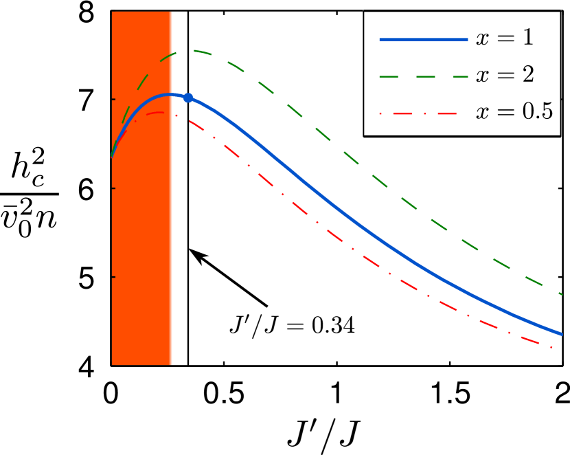
Figure 5: (Color online) Plot of the dimensionless factor $h_{c}^{2}/n\bar{v}^{2}$ appearing in Eqs. (87), and(88) as a function of the ratio $J^{\prime}/J$. To illustrate the dependence on the Dzyaloshinskii-Moriya interaction $D$ we have scaled $D$ with $J^{\prime}$ such that at the experimental value of the ratio $J^{\prime}/J$ (indicated by a vertical line) the experimental value $D_{\text{ex}}$ is given by $D_{\text{ex}}=D/x$. The different curves correspond to different values of $x$ as indicated in the caption, and the dot marks the experimental values of $J$, $J^{\prime}$ and $D$. Quantum fluctuations destroy the long-range order in the triangular lattice antiferromagnet in the shaded area ($J^{\prime}/J\lesssim 0.27$), see Ref. [Trumper, 1999].

Obviously, this factor is maximal if $J^{\prime}/J$ is close to the experimental value $J^{\prime}/J\approx 0.34$. Of course, our mapping between the spin system and the Bose gas is only quantitatively accurate if $h$ is close to $h_{c}$, although for smaller $h$ the qualitative behavior of the dynamic structure factor should still be given by the above expressions. A plot $S^{zz}(\bm{k},\omega)$ for $h=0.7h_{c}$ and for values for $c$ and $\Delta$ relevant for Cs₂CuCl₄ is shown in Fig. 6.

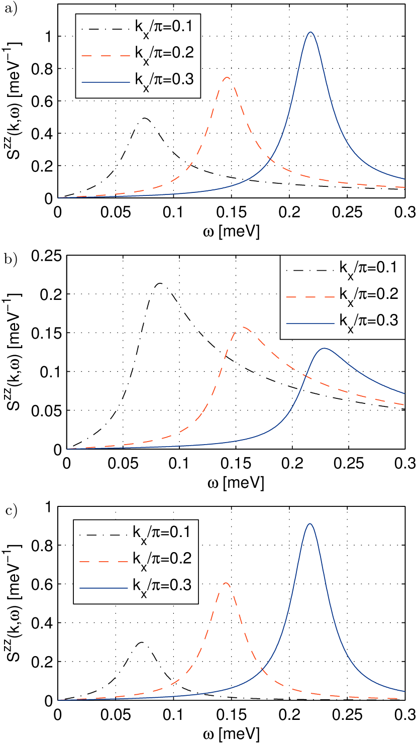
Figure 6: (Color online) Graph of the component $S^{zz}(\bm{k},\omega)$ of the dynamic structure factor in the cone state of Cs₂CuCl₄ along the crystallographic $a$ axis for a magnetic field of magnitude $h=0.7h_{c}$ parallel to the $a$ axis. The curves are for $k_{y}=0$ and different values of $k_{x}$ as indicated in the captions. The upper panel (a) shows the total contribution, the middle panel (b) shows the anomalous contribution given by the first term on the right-hand side of Eq. (86), and the lower panel (c) represents the $\delta$-function contribution given by the last term in Eq. (86). To take into account the typical energy resolution in neutron scattering experimentsColdea et al. (2003) we have convoluted the right-hand side of Eq. (86) with a Lorentzian of width $\gamma=0.019\,\text{meV}$ (full width at half maximum). To fix the parameters $c$, $\Delta$, and $\rho_{0}$ appearing in Eq. (86), we use the large-$S$ relations (77a)-(77c) with $\bar{v}_{0}=374\,\text{m/s}$ (compare Fig. 3) and $n=2/(bc)$ (see Fig. 2). For simplicity we have set $Z_{\parallel}=1$.

The pronounced asymmetry of the spectral line-shape factor shown in the upper panel is due to the threshold singularity of the anomalous contribution shown in the middle panel (b) of Fig. 6.

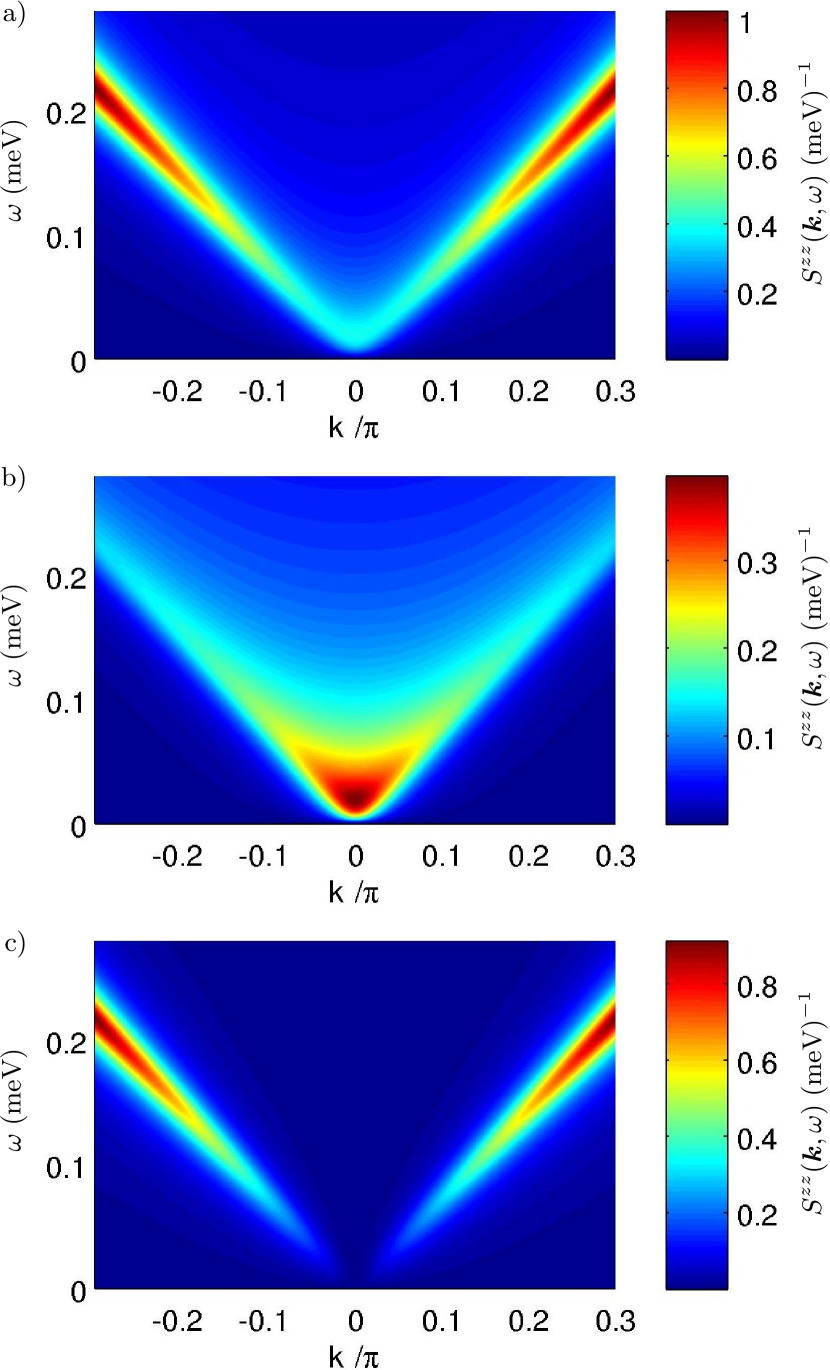
Figure 7: (Color online) Contour plots of the component $S^{zz}(\bm{k},\omega)$ of the dynamic structure factor for $k_{y}=0$. The upper panel (a) shows the total contribution that adds up from the anomalous contribution [middle panel, (b)] and the $\delta$-function contribution [lower panel, (c)]. The parameters and the smoothing procedure are the same as in Fig. 6.

Because the weight of the $\delta$-function peaks in the transverse component of the structure factor in Eq. (85) is a factor of $(\Delta/\omega)^{2}$ larger than the $\delta$-function peak in the longitudinal structure factor (86), whereas the continuum contributions have the same order of magnitude in both components, we conclude that the best way to detect the anomalous scattering continua in Cs₂CuCl₄ is via a measurement of the component $S^{zz}(\bm{k},\omega)$ of the dynamic structure factor along the crystallographic $a$ axis for magnetic fields below but not too close to $h_{c}$. Note that for inelastic neutron scattering with unpolarized neutrons the differential cross section always involves a contribution from the transverse components of the structure factor,Marshall and Lovesey (1971)

$$\frac{d^{2}\sigma(\bm{k},\omega)}{d\omega d\Omega}=|f_{\bm{k}}|^{2}\sum_{\alpha\beta}(\delta_{\alpha\beta}-\hat{k}_{\alpha}\hat{k}_{\beta})S^{\alpha\beta}(\bm{k},\omega)$$ (89)

$$= |f_{\bm{k}}|^{2}\left[(1-\hat{k}_{z}^{2})S^{zz}(\bm{k},\omega)+(1+\hat{k}_{z}^{2})S^{xx}(\bm{k},\omega)\right],\hskip 19.91692pt$$

where $\hat{k}_{\alpha}=k_{\alpha}/|\bm{k}|$ and the magnetic form factor $f_{\bm{k}}$ of the magnetic Cu²⁺ ions in Cs₂CuCl₄ has a rather weak momentum dependence.Coldea et al. (2003) The large $\delta$-function peaks of $S^{xx}(\bm{k},\omega)$ will therefore dominate the neutron-scattering cross section, and it seems rather difficult to detect the nonanalytic scattering continuum with unpolarized neutrons. Note, however, that longitudinal spin fluctuations in nickel have been successfully detected with polarized inelastic neutron scatteringBöni et al. (1991) so that with polarized neutrons the longitudinal structure factor of Cs₂CuCl₄ should be more easily accessible experimentally. Contour plots of the total scattering intensities as well as the anomalous and the $\delta$-function contributions to the dynamic structure factor are shown in Fig. 7. By comparing the upper panel (total intensity) with the lower panel ($\delta$-function contributions as also obtained in the framework of linear spin-wave theory) the effect of the anomalous scattering continua can be seen.

V Summary and conclusions

To summarize, we have shown that in the magnetically ordered ground state of the anisotropic triangular lattice antiferromagnet Cs₂CuCl₄ in a uniform magnetic field along the crystallographic $a$ axis (cone state) the interactions between spin waves lead to infrareddivergent terms in the $1/S$ expansion. These divergencies are generated by the coupling between transverse and longitudinal fluctuations in the ordered phase. Similar singularities are expected to appear in any magnetically ordered spin system with a linear magnon spectrum and a finite triangular vertex involving two powers of the transverse spin-fluctuation field and one power of the longitudinal spin-fluctuation field. The reason why these divergencies have not been noticed in a previous spin-wave calculationVeillette et al. (2005) of the dynamic structure factor of Cs₂CuCl₄ is that in this calculation only the case of vanishing magnetic field has been considered where the relevant triangular vertex vanishes.

We are not aware of any published neutron scattering data probing the dynamic structure factor in the cone state of Cs₂CuCl₄ in an external magnetic field. We predict that in this case the spectral lineshape should exhibit a characteristic anisotropy associated with the threshold divergence proportional to $[\omega^{2}-c^{2}\bm{k}^{2}]^{-1/2}$ of the anomalous contribution. Although in the transverse components of the dynamic structure factor the relative weight of this continuum is rather small, it should be observable in the component $S^{zz}(\bm{k},\omega)$ associated with spin correlations along the crystallographic $a$ axis. Of course, non-singular higher-order terms in the $1/S$ expansion also give rise to extended scattering continua,Veillette et al. (2005) which could overshadow the continua due to the anomalous longitudinal fluctuations. However, sufficiently close to the threshold $\omega=c|\bm{k}|$ the square-root divergence associated with the anomalous longitudinal fluctuations should be the dominant source of asymmetry of the spectral lineshape.

References

- Balents (2010) L. Balents, Nature 464, 199 (2010).
- Coldea et al. (2002) R. Coldea, D. A. Tennant, K. Habicht, P. Smeibidl, C. Wolters, and Z. Tylczynski, Phys. Rev. Lett. 88, 137203 (2002).
- Coldea et al. (2003) R. Coldea, D. A. Tennant, and Z. Tylczynski, Phys. Rev. B 68, 134424 (2003).
- Sytcheva et al. (2009) A. Sytcheva, O. Chiatti, J. Wosnitza, S. Zherlitsyn, A. A. Zvyagin, R. Coldea, and Z. Tylczynski, Phys. Rev. B 80, 224414 (2009).
- Kreisel et al. (2011) A. Kreisel, P. Kopietz, P. T. Cong, B. Wolf, and M. Lang, Phys. Rev. B 84, 024414 (2011).
- Vachon et al. (2011) M.-A. Vachon, G. Koutroulakis, V. F. MitroviÄ, O. Ma, J. B. Marston, A. P. Reyes, P. Kuhns, R. Coldea, and Z. Tylczynski, New J. Phys. 13, 093029 (2011).
- Starykh and Balents (2007) O. A. Starykh and L. Balents, Phys. Rev. Lett. 98, 077205 (2007).
- Kohno et al. (2007) M. Kohno, O. A. Starykh, and L. Balents, Nat. Phys. 3, 790 (2007).
- Starykh et al. (2010) O. A. Starykh, H. Katsura, and L. Balents, Phys. Rev. B 82, 014421 (2010).
- Griset et al. (2011) C. Griset, S. Head, J. Alicea, and O. A. Starykh, Phys. Rev. B 84, 245108 (2011).
- Chen et al. (2013) R. Chen, H. Ju, H.-C. Jiang, O. A. Starykh, and L. Balents, Phys. Rev. B 87, 165123 (2013).
- Herfurth et al. (2013) T. Herfurth, S. Streib, and P. Kopietz, Phys. Rev. B 88, 174404 (2013).
- Mermin and Wagner (1966) N. D. Mermin and H. Wagner, Phys. Rev. Lett. 17, 1133 (1966).
- Nepomnyashchii and Nepomnyashchii (1978) Y. A. Nepomnyashchii and A. Nepomnyashchii, JETP 48, 493 (1978).
- Popov and Seredniakov (1979) V. Popov and A. Seredniakov, JETP 50, 193 (1979).
- Weichman (1988) P. B. Weichman, Phys. Rev. B 38, 8739 (1988).
- Giorgini et al. (1992) S. Giorgini, L. Pitaevskii, and S. Stringari, Phys. Rev. B 46, 6374 (1992).
- Castellani et al. (1997) C. Castellani, C. Di Castro, F. Pistolesi, and G. C. Strinati, Phys. Rev. Lett. 78, 1612 (1997).
- Pistolesi et al. (2004) F. Pistolesi, C. Castellani, C. Di Castro, and G. C. Strinati, Phys. Rev. B 69, 024513 (2004).
- Sachdev (1999) S. Sachdev, Phys. Rev. B 59, 14054 (1999).
- Zwerger (2004) W. Zwerger, Phys. Rev. Lett. 92, 027203 (2004).
- Kreisel et al. (2007) A. Kreisel, N. Hasselmann, and P. Kopietz, Phys. Rev. Lett. 98, 067203 (2007).
- Dupuis (2011) N. Dupuis, Phys. Rev. E 83, 031120 (2011).
- Maleyev (2000) S. V. Maleyev, Phys. Rev. Lett. 85, 3281 (2000).
- Syromyatnikov and Maleyev (2001) A. V. Syromyatnikov and S. V. Maleyev, Phys. Rev. B 65, 012401 (2001).
- Hasselmann and Kopietz (2006) N. Hasselmann and P. Kopietz, Europhys. Lett. 74, 1067 (2006).
- Kreisel et al. (2008) A. Kreisel, F. Sauli, N. Hasselmann, and P. Kopietz, Phys. Rev. B 78, 035127 (2008).
- Holstein and Primakoff (1940) T. Holstein and H. Primakoff, Phys. Rev. 58, 1098 (1940).
- Veillette et al. (2005) M. Y. Veillette, A. J. A. James, and F. H. L. Essler, Phys. Rev. B 72, 134429 (2005).
- Trumper (1999) A. E. Trumper, Phys. Rev. B 60, 2987 (1999).
- Note (1) Note that the lower bound is determined by a critical ratio where quantum fluctuations in the leading order of the expansion destroy long range order; the case is just the well-known case of the Heisenberg chain in one dimensionMermin and Wagner (1966).
- Note (2) As discussed in Ref. \rev@citealpnumTrumper99, the triangular antiferromagnet is in a spiral state for with an ordering vector that is a continuous function of and . Allowing to be outside of the first Brillouin zone one can assume . The true physical value of the ordering vector can then be obtained by shifting with the reciprocal vector .
- Shi and Griffin (1998) H. Shi and A. Griffin, Phys. Rep. 304, 1 (1998).
- Andersen (2004) J. O. Andersen, Rev. Mod. Phys. 76, 599 (2004).
- Sinner et al. (2009) A. Sinner, N. Hasselmann, and P. Kopietz, Phys. Rev. Lett. 102, 120601 (2009).
- Sinner et al. (2010) A. Sinner, N. Hasselmann, and P. Kopietz, Phys. Rev. A 82, 063632 (2010).
- Marshall and Lovesey (1971) W. Marshall and S. W. Lovesey, Theory of thermal neutron scattering: the use of neutrons for the investigation of condensed matter (Clarendon Press Oxford, 1971).
- Böni et al. (1991) P. Böni, J. L. Martinez, and J. M. Tranquada, Phys. Rev. B 43, 575 (1991).