The Atacama Cosmology Telescope: CMB Polarization at $200<\ell<9000$

Abstract

We report on measurements of the cosmic microwave background (CMB) and celestial polarization at 146 GHz made with the Atacama Cosmology Telescope Polarimeter (ACTPol) in its first three months of observing. Four regions of sky covering a total of 270 square degrees were mapped with an angular resolution of $1.3^{\prime}$. The map noise levels in the four regions are between 11 and 17 $\mu$K-arcmin. We present TT, TE, EE, TB, EB, and BB power spectra from three of these regions. The observed E-mode polarization power spectrum, displaying six acoustic peaks in the range $200<\ell<3000$, is an excellent fit to the prediction of the best-fit cosmological models from WMAP9+ACT and Planck data. The polarization power spectrum, which mainly reflects primordial plasma velocity perturbations, provides an independent determination of cosmological parameters consistent with those based on the temperature power spectrum, which results mostly from primordial density perturbations. We find that without masking any point sources in the EE data at $\ell<9000$, the Poisson tail of the EE power spectrum due to polarized point sources has an amplitude less than $2.4$ $\mu$K² at $\ell=3000$ at 95% confidence. Finally, we report that the Crab Nebula, an important polarization calibration source at microwave frequencies, has 8.7% polarization with an angle of $150.7^{\circ}\pm 0.6^{\circ}$ when smoothed with a $5^{\prime}$ Gaussian beam.

1. Introduction

The standard $\Lambda$CDM model of cosmology is now well established (e.g., Spergel et al., 2003; Planck Collaboration, 2013c). The model is geometrically flat and dark-energy dominated, with baryons comprising about 15% of the total matter density. The initial fluctuations are adiabatic, Gaussian, and nearly scale-free. The free parameters of the model have been determined to high precision, largely from measurements of the cosmic microwave background (CMB) temperature anisotropies on angular scales from the full sky down to a few arcminutes (Hinshaw et al., 2013; Planck Collaboration, 2013c; Sievers et al., 2013; Hou et al., 2014). Large-scale structure measurements of the baryon acoustic oscillation scale (e.g., Anderson et al., 2014) and direct measurements of the expansion rate and acceleration from type-Ia supernova observations (e.g., Suzuki et al., 2012; Betoule et al., 2014) also provide constraints. While the model is in generally good agreement with all cosmological probes, there are some mild tensions at the $2\sigma$ to $3\sigma$ level (e.g., Planck Collaboration, 2013c) and possible hints of “anomalies” (e.g., Planck Collaboration, 2013d; Bennett et al., 2011; Copi et al., 2010). Further precise tests of the model are clearly needed.

The polarization of the CMB provides a complementary source of information and also probes cosmological physics beyond what can be obtained with temperature alone. The E-mode polarization power spectrum (Kamionkowski et al., 1997; Zaldarriaga & Seljak, 1997) arises primarily from the motions of the primordial plasma at the epoch of last scattering (redshift $z=1100$), with a contribution at large angular scales from perturbations at the reionization epoch ($z\approx 10$). Precision measurements of the acoustic features in the E-mode polarization power spectrum provide a non-trivial confirmation of the acoustic oscillations in the early universe seen in temperature data. Rocha et al. (2004) and Galli et al. (2014) point out that with the CMB E-mode polarization alone one may place stronger constraints on cosmological parameters than with the temperature anisotropy. More importantly, the combination of temperature and polarization data constrain a range of physical effects beyond the standard model. For example, primordial isocurvature perturbations alter the phase of the oscillations in polarization relative to temperature compared to pure adiabatic perturbations (e.g., Bond & Efstathiou, 1987; Bucher et al., 2004; MacTavish et al., 2006; Sievers et al., 2007). The additional sensitivity to the standard cosmological model provides increased ability to probe neutrino properties, early dark energy, and time variation of fundamental constants. Comparison of temperature and polarization data also probes cosmological effects which affect the two in different ways, such as the kinematic Sunyaev-Zeldovich effect (Calabrese et al., 2014).

Polarization observations can also characterize the B-mode fluctuations, which are not generated by the dominant primordial density perturbations. B-mode polarization contains a signal from gravitational lensing by all structure along the line of sight, for multipoles $\ell>200$ (Zaldarriaga & Seljak, 1998). The B-mode fluctuations also reflect other new physical effects, such as cosmic birefringence due to magnetic fields (Kosowsky et al., 2005) or photon couplings beyond the standard model (Lue et al., 1999). A definitive detection of primordial B-mode polarization at $\ell<200$ from tensor perturbations generated by inflation will test the fundamental nature of the gravitational force and probe energy scales well beyond terrestrial experiments.

Although WMAP has made the only published measurement of large-angle E-mode polarization at $\ell<15$, measurements of polarization with $\ell>15$ have steadily improved. The Planck team has shown excellent visual agreement between their best-fit $\Lambda$CDM model and their TE and EE polarization spectra for $\ell\geq 100$ but has not yet quantified the agreement (Planck Collaboration, 2013c, Figure 11). On larger angular scales, $30<\ell<1000$, the CAPMAP (CAPMAP Collaboration, 2008), QUAD (QUaD Collaboration, 2009), QUIET (QUIET Collaboration, 2012), and BICEP (BICEP1 Collaboration, 2013) teams have shown, along with WMAP (Hinshaw et al., 2013), that the predicted E-mode signal is in quantitative agreement with the $\Lambda$CDM prediction. In addition, they placed limits on primordial and lensing B-modes. Through cross correlating the EB-reconstructed lensing signal with the Herschel-SPIRE maps, SPT (Hanson et al., 2013) demonstrated the presence of lensing B-mode polarization at $7.7\sigma$. In a similar cross-correlation analysis, the Polarbear team found $2.3\sigma$ evidence (Polarbear Collaboration, 2013) for lensing B-modes and also demonstrated the presence of lensed B-mode polarization through the EEEB and EBEB four-point functions at $4.2\sigma$ (Polarbear Collaboration, 2014). Following that, Polarbear released their measurements of the TT, TE, and EE power spectra, $2\sigma$ evidence of non-zero BB power, and limits on the TB and EB spectra (Polarbear Collaboration, 2014). Most recently, the BICEP2 team released their $7\sigma$ detection of degree angular-scale B-mode polarization along with a suite of related spectra (BICEP2 Collaboration, 2014a).

This paper is the Atacama Cosmology Telescope (ACT) collaboration’s first step in measuring CMB polarization and is organized as follows. In §2 we introduce the salient features of the instrument and then in §3 describe the observations and data reduction. In §4 we present our power spectra measurements and interpretation, and conclude in §5. For power spectra, we use the Planck notation: ${\cal D}^{\rm{XY}}_{\ell}=\ell(\ell+1)C^{\rm XY}_{\ell}/2\pi$ where ${\rm XY}\in{{\rm TT,\,TE,\,TB,\,EE,\,EB,\,BB}}$. We do not consider circular polarization (e.g., Alexander et al., 2009; Cooray et al., 2003). The maps are made in J2000 equatorial coordinates. We adopt the HEALPIX (Górski et al., 2005) convention for Stokes parameters Q and U. Polarization position angles respect the IAU convention (see, e.g., Hamaker & Bregman, 1996), increasing from North towards East, and thus are computed as $\gamma_{p}=(1/2)\text{arg}(Q-iU)$. We note that these are the same conventions adopted by Planck (see, e.g., Section 2.1 of Planck Collaboration, 2014), although Planck uses Galactic coordinates.

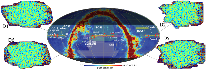
Figure 1.— ACTPol maps and overlapping surveys. The maps have been filtered to emphasize $\ell>300$. The power spectra are obtained with only the high S/N region of each map. Going from left to right across the equator, the red circles indicate patches D1, D6, D5, D4, D3 and D2 (the first ACTPol season focused on D1, D2, D5 and D6). More than half the sky, as indicated by the light colored area, is accessible to ACTPol. Overlapping surveys include SDSS (SDSS, 2014), BOSS(BOSS, 2014), CFHTLS (CFHTLens Collaboration, 2013), XMM-XXL (XMM-XXL, 2014), Herschel (HerMES & HeLMS, Oliver et al. (2012); Viero et al. (2014)), HSC (Subaru, 2014), DES (DES, 2014), GAMA (Driver et al., 2009), and KiDS (de Jong et al., 2013).

2. The Instrument

ACT is located at latitude 22^∘57^′31^′′S and longitude 67^∘47^′15^′′W at an altitude of 5190 m in Parque Astronómico Atacama in northern Chile. The 6 m primary mirror leads to arcminute resolution at millimeter wavelengths. A first-generation receiver, the Millimeter Bolometric Array Camera (MBAC; Fowler et al., 2007; Swetz et al., 2011), observed from Sept. 2007 through Dec. 2010. It was decommissioned and replaced by the polarization-sensitive ACTPol camera (Niemack et al., 2010) in 2013.

ACTPol is similar to MBAC in a number of ways: it has three separate “optics tubes” each of which terminates in an independent detector array; it uses three antireflection coated silicon lenses per tube to feed the detectors; it is located at the Gregorian focus of the telescope and illuminates the 2 m diameter secondary; the passbands are defined in part by free-space filters (Ade et al., 2006); IR radiation is blocked with free-space filters (Tucker & Ade, 2006); and the transition-edge-sensor (TES) detectors are read out by time-division SQUID multiplexing (Chervenak et al., 1999), which is implemented using the Multi-Channel Electronics (MCE, Battistelli et al., 2008). ACTPol differs from MBAC in that the antireflection coating is achieved through a “metamaterial” (grooving of a silicon lens surface; Datta et al., 2013); cryogenic corrugated silicon horns feed two orthogonal polarizations (Britton et al., 2010; Hubmayr et al., 2012); the lower edge of the spectral passband is determined by the feed structure’s input waveguide cutoff frequency, while the upper end is defined by free-space filters; the detector arrays (Grace et al., 2014; Pappas et al., 2014) are cooled to 100 mK as opposed to 300 mK; and a continuous dilution refrigerator cools the detector arrays instead of a ³He sorption refrigerator, which enables daytime observations. The receiver is 40% larger than MBAC in volume.

Two of the optics tubes are designed to operate at 146 GHz and have 522 feeds (1044 TES detectors) each, 506 of which are typically used. In addition to the optical detectors, there are 6 dark detectors and 6 resistors for noise tests. The third tube will use a 90/146 GHz dichroic detector array with broad-band cold optics (Datta et al., 2014) and have 1020 TES detectors coupled to 255 feeds. For the results reported here, only one 146 GHz tube was installed. The second 146 GHz tube was installed in 2014 with the final tube scheduled for early 2015.

The array sensitivity (relative to the CMB) of the 2013 observations with the first optics tube is $\sim 19\,\mbox{$\mu{\rm K}\sqrt{\rm s}$}$. For comparison, the MBAC sensitivity at 148 GHz was $32\,\mbox{$\mu{\rm K}\sqrt{\rm s}$}$. The 405 most sensitive detectors provide 95% of the statistical weight in the maps, and the in situ median detector sensitivity is $340\,\mbox{$\mu{\rm K}\sqrt{\rm s}$}$ (Grace et al., 2014). Substantial improvements in sensitivity for 2014 observations are expected due to the unusually high precipitable water vapor (PWV) in 2013, reductions in readout noise, reduced background loading, as well as the addition of new detector arrays.

The response of the ACTPol detectors diminishes with frequency such that it has a loading-dependent $f_{\rm 3dB}$ (the frequency at 50% of the peak response) of 10-200Hz. When accounting for our scan speed and observing strategy, $f_{\rm 3dB}=70$ Hz corresponds to a rolloff in the angular power spectrum of 3% at $\ell=3000$. The individual $f_{\rm 3dB}$ frequencies of the detectors, including their dependence on loading from the changing elevation and precipitable water vapor (PWV), are accounted for in the analysis, although it contributes only a few percent (0.1% at $\ell=3\,000$; 2% at $\ell=10\,000$) difference in the power spectra compared to assuming the median value.

The passbands of the detectors were determined in the laboratory, before deployment, with a Fourier Transform Spectrometer. An effective frequency for the CMB $\nu_{\rm CMB}=146\pm 3$ GHz was measured and we adopt this throughout the analysis. The error bar is systematic, and will improve after planned measurements of the passband in the field. The resulting conversion between CMB and Rayleigh-Jeans equivalent source temperatures is $\delta T_{CMB}/\delta T_{RJ}=1.66\pm 0.04$. The Dicke bandwidth (Dicke, 1946) is $\Delta\nu=49$ GHz.

3. The observations and data reduction

3.1. Sky coverage and scan strategy

ACTPol data are acquired by scanning the telescope in azimuth at a variety of different elevations. A patch is scanned as it rises in the east and then again as it sets in the west. In this first year, we concentrated on four “deep fields” approximately centered on the celestial equator at right ascensions $150^{\circ}$, $175^{\circ}$, $355^{\circ}$ and $35^{\circ}$ which we call D1 (73 deg²), D2 (70 deg²), D5 (70 deg²) and D6 (63 deg²) respectively. The areas refer to the deep, rectangular regions with even coverage in the center of each patch that we use for power spectrum analysis. These patches were chosen for their overlap with other surveys and are shown in Figure 1. The separation of the patches is such that only one is visible at any given time, and in a typical 24 hour period all four patches were observed in sequence unless the observation would require the telescope to point within five degrees of the Sun. With our scan strategy, each patch is observed in a range of different parallactic angles while scanning horizontally. This is important for separating instrumental from celestial polarization and is a benefit of observing from a non-polar site.

The CMB fields are observed by scanning at $1.5^{\circ}$/s in azimuth, turning around in 1 s, scanning back to the original position, turning around in 1 s and repeating. The duration of the scan depends on elevation; a full cycle takes 16.4 s at an elevation of $35^{\circ}$ and 20.9 s at $60^{\circ}$. This is done for 60 scans, or roughly 10 minutes, to form a time-ordered-data or “TOD” packet. The elevation is sometimes changed between 10 minute scans, at which point the detector bias is modulated to recalibrate and check for any changes in the time constants due to the change in sky load.

Data for the maps in Figure 1 were taken from Sept. 11, 2013 to Dec. 14, 2013. During this time, in addition to observing the CMB, we performed a number of systematic checks, characterized the instrument, observed planets, and observed the Crab Nebula (Tau A). The net amount of time that went into the maps was 236, 178, 311, and 305 hours for D1, D2, D5, D6 respectively. This represents 24%, 16%, 29% and 31% of the total CMB observation time. However, we use only the lowest noise regions of the maps, which constitute around $70\%$ of the total observing time. This results in a white noise map sensitivity, in the sense of Figure 2 in Das et al. (2014), of 16.2, 17, 13.2, and 11.2 $\mu$K-arcmin respectively. For Stokes $Q$ or $U$ sensitivities these numbers should be multiplied by $\sqrt{2}$.

We divide the data into “day” (11:00-24:00 UTC) and “night” (0:00-11:00 UTC). The nighttime data fraction for patches D1, D2, D5 and D6 is 50%, 25%, 76% and 94% respectively. For this analysis we use only the nighttime data from D1, D5, and D6, amounting to 63% of the total.

3.2. Beam, pointing, and polarization reconstruction

We have found that multiple observations of planets (Hincks et al., 2010; Hasselfield et al., 2013) are essential for determining the beam profile. In 2013 Uranus was observed 120 times and analyzed as in Hasselfield et al. (2013). With all detectors combined, regardless of polarization, the beam is slightly elliptical with FWHM of $1.36^{\prime}$ ($1.26^{\prime}$) along the major (minor) axis. The solid angle is $\Omega_{B}=194\pm 6$ nsr ($2.29\pm 0.07$ arcmin²), before any smearing due to pointing. These results agree up to $\ell=5000$ with a similar analysis of 20 observations of Saturn, a much brighter source. We did not detect any significant deviations when the data were split by the elevation of observation or whether the source was rising or setting. The beam profile was marginally detected in polarization maps of Uranus made in coordinates fixed to the optical system. Since the observations probed the planet at a range of parallactic orientations, this signal is interpreted as either $I$ to $P$ leakage in the optics or due to the analysis pipeline. The leakage from $I$ to $P$ due to this effect is less than $1.5\%$ at $\ell<5000$. The leakage is dominated by monopole terms and thus is highly suppressed in CMB maps because a range of parallactic angles is explored by the cross-linking scan strategy. Including the effects of cross-linking in the analysis of Uranus, we find the polarized fraction of the 146 GHz emission from Uranus to be less than 0.8% at 95% confidence.

A simple telescope pointing model is constrained using observations of planets at night. This model allows the pointing to be reconstructed with an rms error of $14^{\prime\prime}$. The impact of pointing variance on the full season CMB maps is handled as in Hasselfield et al. (2013), leading to effective beams in the CMB maps with solid angle $\Omega_{B}=224\pm 20$ nsr for D1, $\Omega_{B}=234\pm 14$ nsr for D5, and $\Omega_{B}=224\pm 12$ nsr for D6. The uncertainties include both beam and pointing contributions.

Average pointing error in the full season maps is assessed by comparing point source positions to the FIRST catalog (Becker et al., 1995; White et al., 1997). The absolute pointing error rms is found to be $5^{\prime\prime}$ in the nighttime maps, with no significant deviations when the data are split by elevation or time of observation. A $7^{\prime\prime}$ offset in the absolute pointing is uncorrected in this analysis.

Detectors co-located in the focal plane may point at slightly different positions on the sky, an effect seen by the BICEP2 Collaboration (2014b) at the $1^{\prime}$ level. Because our detector pointing offsets are individually measured, and the map making procedure does not difference detectors directly (§3.4), this is not a primary concern for us but it is an important check of the instrument. From the analysis of planet observations, we find that the optical axes of a typical detector pair differ by less than $3^{\prime\prime}$.

During the day, the heat from the Sun distorts the telescope structure. The distortion pattern is repeatable, although we currently cut data between 17:00 and 20:00 UTC (13:00 and 16:00 local time) when the distortion is greatest. The distortion leads to two effects: the first is a pointing offset and the second is a repeatable deformation of the reflector, which changes the shape of the beam. Both of these effects lead to a roll-off in $\ell$ that resembles a low pass filter and can be treated as a beam effect in the likelihood. We do not include the daytime data in our cosmological parameter analysis, as models for the daytime beam response are still in development. Nevertheless, our preliminary treatment of the daytime beam produces power spectra that are consistent with nighttime spectra (Figure 5) and pass null tests (see §4.1).

Each detector is sensitive to a single linear polarization direction, and the relative angles of the detectors within each array are set by lithography during fabrication. The optical detector orientations are calculated by raytracing through the full optical system to determine the projection of each detector within an array on the sky.

CMB temperature fluctuation measurements from Planck and WMAP are used to calibrate the ACTPol T, Q, and U maps with a common rescaling factor, as described in §4. However, signal in the Q and U maps will be attenuated by an additional factor $\alpha_{\text{P}}$, which is different from unity due primarily to errors in the assumed detector polarization angles. For the present analysis we take $\alpha_{\text{P}}=0.95\pm 0.05$; this is discussed further in §3.3.

Any mean offset between the assumed and actual detector polarization angles must be understood in order to properly decompose polarized intensity into E and B components. The polarized CMB may be used to assess the offset angle under the assumption that the intrinsic correlation between the E and B signals is zero. Systematic optical effects associated with polarization, including parallactic rotations, cause a leakage from E to B modes and induce spurious signal in EB and TB correlations (e.g., Shimon et al. 2008). The most likely instrument polarization reference angle may thus be determined by minimizing the inferred EB signal with respect to offset angle (e.g., Keating et al. 2013). Under these assumptions, the ACTPol E and B spectra from $500<\ell<2000$ constrain the instrumental polarization offset angle to be $\delta\gamma_{p}=-0.2^{\circ}\pm 0.5^{\circ}$. This result is referred to as the EB-nulling offset angle. Since this angle is small and consistent with zero, we do not correct the spectra for this effect in the present analysis. The agreement with zero suggests that the optical modeling procedure is free of systematic errors at the $0.5^{\circ}$ level or better.

Naturally, estimating the polarization offset angle by assuming E and B to be uncorrelated eliminates sensitivity to models, such as isotropic cosmic birefringence, where the distinguishing characteristic is a constant EB cross-correlation. As an alternative calibration approach, measurements of the polarized signal from a bright astrophysical source may be compared to values from the literature. The Crab Nebula is a convenient source for this purpose.

3.3. The Crab Nebula

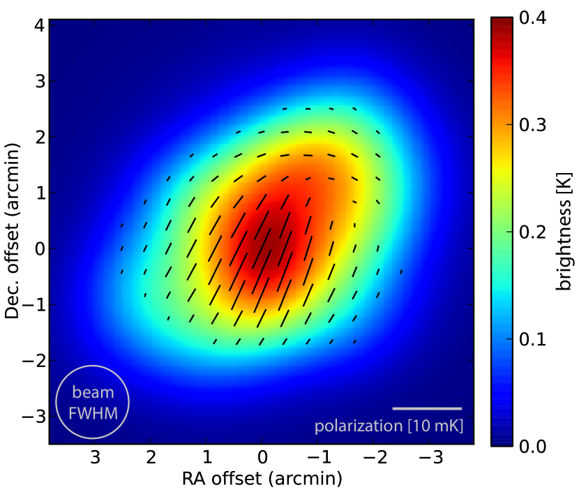
Figure 2.— ACTPol intensity and polarization map of the Crab Nebula (Tau A). The brightness scale is in differential temperature units, relative to the CMB at 146 GHz (for Rayleigh-Jeans brightness temperature, divide by 1.66). Black bars show polarization direction, with length proportional to polarized intensity ($(Q^{2}+U^{2})^{1/2}$), which reaches a maximum of 6.8 mK. The origin of the coordinate system corresponds to the Crab Pulsar position. Note the variation in polarization angle and fraction across the source, which complicates the use of the source as a precision calibrator. Polarization features are in good qualitative agreement with the higher resolution, 89.2 GHz maps of Aumont et al. (2010); a numerical comparison is discussed in the text. This map has been resampled to $2^{\prime\prime}$ pixels from its original $30^{\prime\prime}$ resolution but has not otherwise been smoothed.

The Crab Nebula, or Tau A, is an extended polarized supernova remnant whose emission below $\approx 1$ THz is dominated by synchrotron radiation (see, e.g., Hester, 2008). Its brightness and compactness provide a convenient polarization reference for millimeter-wavelength observatories. From WMAP measurements at 93 GHz, Tau A is polarized in the direction $\gamma_{p}=148.9^{\circ}\pm 1.8^{\circ}$ in equatorial coordinates (Weiland et al., 2011). These agree with the IRAM observations at 89.2 GHz which give the direction as $\gamma_{p}=149.9^{\circ}\pm 0.2^{\circ}$ when smoothed to a $5^{\prime}$ Gaussian beam (Aumont et al., 2010).

Tau A was observed roughly every second day during the 2013 observing season. A co-added map from a subset of these observations is shown in Figure 2. The results presented here are a preliminary analysis with the goal of demonstrating the level to which the polarization sensitivity of the instrument is understood.

Because of their $27^{\prime\prime}$ resolution and higher precision, we take the IRAM results as our reference. We downgrade the resolution of the ACTPol maps to match a $5^{\prime}$ Gaussian beam and compare to the Aumont et al. (2010) values for this case. The difference corresponds to an instrument polarization offset angle of $\delta\gamma_{p}=-1.2^{\circ}\pm 0.2^{\circ}$ at the pulsar position in the smoothed maps, where the uncertainty is statistical and is assessed by comparing three independent sets of ACTPol observations.

The analysis of Tau A was performed while keeping the EB result “blinded,” and provides an independent probe of the instrumental polarization offset angle. With the EB result unblinded, the difference between the IRAM-based and EB-nulling polarization offset angles is $1.0^{\circ}\pm 0.5^{\circ}$. This difference is consistent with the $1.1^{\circ}\pm 0.5^{\circ}$ offset found by Polarbear Collaboration (2014) at 150 GHz, and increases the evidence of a $\approx 1^{\circ}$ difference in Tau A polarization between 90 and 150 GHz. (The uncertainty stated here for the Polarbear result does not include a contribution from IRAM overall polarization uncertainty.)

Studies of the total flux density of the nebula have shown that the spectrum is well described by a single synchrotron component (Macías-Pérez et al., 2010), and predict negligible variations in polarization fraction and angle at 150 GHz. However, high resolution studies of the source at 150 GHz and 1.4 GHz demonstrate non-negligible variations of the spectral index over the surface of the source (Arendt et al., 2011). Since the polarization angle also varies over the source, the total polarized flux and mean polarization angle may have a non-trivial behavior as a function of frequency.

Our understanding of the polarization efficiency is currently limited by uncertainty in individual detector polarization angles. Comparison of individual detector timestreams to the ACTPol Tau A maps provides limits on these angle errors. At the present time we can only conclude that the polarization efficiency $\alpha_{\text{P}}$ is at least 0.9, corresponding to an rms uncertainty in the polarization angles of $10^{\circ}$. While this is somewhat larger than the expected deviations, for the present analysis we consider the full range $0.9<\alpha_{\text{P}}<1.0$. In the cosmological likelihood analysis, the efficiency is given a uniform prior over this interval. When stating polarization fractions below, we simply take $\alpha_{\text{P}}=0.95\pm 0.05$ and treat the error as Gaussian.

For the purposes of stating our measurements of the Tau A polarization signature, we apply the EB-nulling instrumental polarization offset. These results apply at 146 GHz, for an instrument with a $5^{\prime}$ Gaussian beam. At the pulsar position, the polarization fraction is $(9.2\pm 0.5)\%$ and the polarization angle is $150.9^{\circ}\pm 0.5^{\circ}$ East of North. At the peak of the smoothed intensity (which lies $22^{\prime\prime}$ northwest of the pulsar position), the polarization fraction is $(8.7\pm 0.4)\%$ at an angle of $150.7^{\circ}\pm 0.6^{\circ}$.

3.4. Data selection and pre-processing

The data selection closely follows the path laid out in Dünner et al. (2013). The main difference in the TOD processing is the procedure for calibrating each detector, as a larger fraction of the detectors are operating near the saturation level. A set of reliable detectors is used to determine an absolute calibration level that is stable over variations in detector temperature and loading. A low-order polynomial is removed from each time stream to limit the impact of low frequency drifts. Then a per-TOD flat-fielding is performed on all the detectors, using the common-mode signal from the atmosphere. At this point the properties of the detector time streams are characterized and screened. The output of this step in the pipeline, which we call the cuts package, is a list of science grade detectors with $f_{3\textrm{dB}}>20\textrm{Hz}$, well-behaved noise, and a common relative calibration. In addition, we reject data when the PWV$>3$ mm. Note that the polarization orientation of a detector does not enter into the data selection or flat-fielding. The time stream processing (such as polynomial removal) used to determine the cuts and calibration are not the same as those applied to the data during mapmaking.

Figure 3.— Example maps from the region $29.65^{\circ}<\textrm{RA}<40.49^{\circ}$ (horizontal), $-7.60^{\circ}<\textrm{Dec}<-0.68^{\circ}$ (vertical), in the center of patch D6. Panels 1,2,3,5,6 (left to right, top to bottom) show T, Q, U, E and B respectively. Panel 4 is a zoom on a $2.79^{\circ}\times 1.73^{\circ}$ subregion of the T map, showing the full map resolution. The maps have been bandpass filtered to maximize signal-to-noise ($240<\ell$ for temperature, $260<\ell<1370$ for polarization). The visible patterns in the Q and U maps are consistent with a sky dominated by E-mode polarization, as can be seen in the derived E and B maps. The B map is consistent with noise except for a faint $m=0$ (constant declination) ground residual (see §3.6). We do not use $m=0$ modes in the power spectrum estimation. See Figure 4 for an illustration of the noise properties in these filtered maps. The circled galaxy cluster candidate, ACT-CL J0205.2-0439, is within $2^{\prime}$ of a CFHTLS cluster candidate with photometric redshift $z=1.1$ (Durret et al., 2011) and three concordant galaxies with spectroscopic $z=0.97$ found in the VIMOS Public Extragalactic Survey (Garilli et al., 2014). The circled point source may be associated with FBQS J0209-0438, a quasar at $z=1.128$ (Véron-Cetty & Véron, 2006).

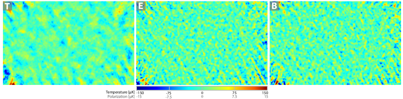
Figure 4.— Difference maps (odd vs. even pairs of nights) for the same region as Figure 3, illustrating the noise properties of the map. Correlated noise is visible as diagonal stripes aligned with our dominant scanning directions (diagonally in these coordinates). These are the map-space equivalent of the correlated noise in the time-ordered data. Noise correlations are taken into account in the noise model in the power spectrum estimation.

3.5. Map making

After applying the cuts, the time-ordered data are projected on the sky by solving the maximum-likelihood map making equation for a vector of map pixels $\mathbf{m}$,

$$A^{T}N^{-1}A\mathbf{m}=A^{T}N^{-1}\mathbf{d},$$ (1)

via the preconditioned Conjugate Gradients algorithm. Here $\mathbf{d}$ is the set of time-ordered data, $N$ is the noise covariance of $\mathbf{d}$ and $A$ is the generalized pointing matrix that projects from map domain to time domain. This follows the method used in Dünner et al. (2013), but extends it to polarization. Polarization is handled by including each detector’s response to the I, Q and U Stokes parameters in the pointing matrix, so the analysis does not depend on explicit detector pair differencing. This approach, coupled with the parallactic angle coverage of our scan strategy, naturally suppresses monopole and dipole polarization leakages. The different noise properties for temperature and polarization are represented as detector correlations in the noise covariance matrix, which we model as stationary in $10$ minute chunks and measure from the data. To avoid bias from applying the noise model to the same data it is measured from, we make a second pass where the estimated sky map is subtracted from the time-ordered data before the noise model is reestimated.

In principle, maximum-likelihood map making results in unbiased, minimum-variance sky maps. But there are a few caveats. With the Conjugate Gradients technique, the number of steps needed to solve for each eigenmode depends on its eigenvalue, and some degenerate or almost degenerate modes never converge. The nature of the degenerate modes depends on the patch size and scanning pattern, but in the present analysis they correspond to the low signal-to-noise modes at multipoles $l\lesssim 50$. Additionally, our current treatment of ground pickup results in a bias on these large scales (see §3.6).

With our current data set, each 70 deg² map is a reduction of $\sim 10^{11}$ samples into $\sim 10^{6}$ pixels, making this the most computationally intensive step in the analysis. Nevertheless, due to the short observation time so far, the costs are still relatively modest compared to the original ACT analysis. Figure 3 shows an example map from patch D6. For display purposes, a bandpass filter has been applied to maximize signal-to-noise. Example difference maps (odd vs. even pairs of nights) for the same region are shown in Figure 4.

3.6. Ground, lunar, and solar pickup

ACT has two levels of ground screens. One screen is fixed to the telescope and scans with it. This entire system sits inside a second 13 m high fixed ground screen. Nevertheless, we still detect a spurious signal which we interpret as ground pickup. When the telescope points to the northeast between azimuths $\sim 25^{\circ}-85^{\circ}$ we observe a spurious signal with a $\sim 30^{\circ}$ period in azimuth, with little elevation dependence, and a peak-to-peak amplitude of $\sim 200\mu$K in Q and U. This is consistent with signal from the nearby mountain Cerro Toco being diffracted over the top of the ground screen’s $30^{\circ}$ wide panels. While this signal is washed out when projected on the sky, it would still be a contaminant of $\pm 20\mu$K or more in our polarization maps if ignored.

The ground signal can be disentangled from the sky because it is constant in azimuth during a scan and does not rotate with parallactic angle like the sky. The exceptions are modes on the sky that depend only on declination, not right ascension (such as the spherical harmonics with $m=0$). These show up as pure functions of azimuth during a constant elevation scan, and are degenerate with the ground even when observing at multiple azimuths and elevations. The remaining modes could, in principle, be disentangled, but in the current analysis we remove both these and the degenerate modes by applying an azimuth filter to the time-ordered data and excluding Fourier modes with $|\ell_{y}|<50$ from the power spectrum estimation.

While the filters are effective at suppressing the ground pickup, they also remove some bona fide sky signal, making our maps and power spectra slightly biased. The effects of the filtering are assessed by passing simulated maps of the polarized CMB through the filtering procedure, and comparing the power spectra of the input and output maps. The main effect of the filter is to suppress, slightly, the signal in temperature (polarization) on large angular scales, with a transfer function that decreases from 0.995 (0.99) at $\ell=500$ to 0.95 (0.9) at $\ell=200$. Leakage from E to B is also seen, but at a level that is negligible for this analysis. Our simulations show that with a more sophisticated treatment we can expect a significantly reduced impact from ground signals in future ACTPol results.

We investigate the possibility of contamination from sidelobes overlapping the Sun or Moon by making maps in coordinates centered on these objects. We identify two sidelobes this way, one around $20^{\circ}$ away from the boresight, and another one $120^{\circ}$ away. These have an amplitude of around $200\mu$K in polarization for the Sun, but are not detected for the Moon. Based on this, we cut all scans that hit these regions in Sun-relative coordinates. As a precautionary measure, we also cut all scans within $10^{\circ}$ of the Moon, which results in a negligible loss of data.

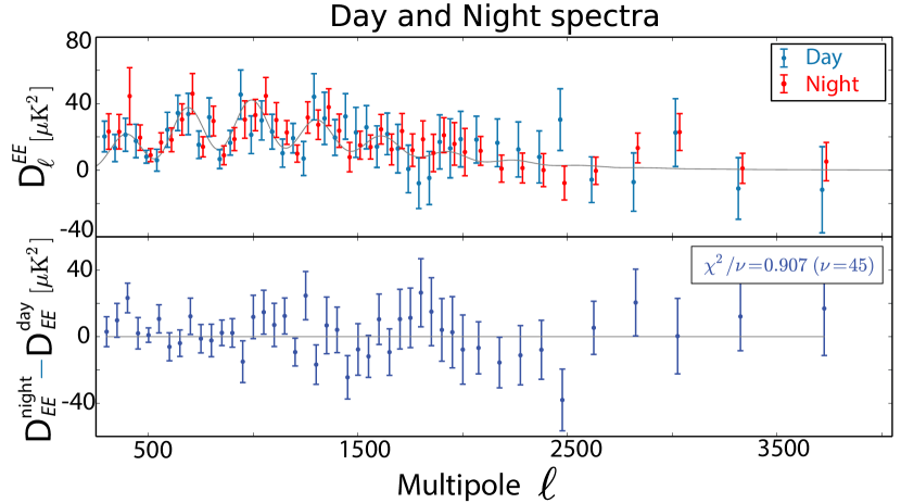
Figure 5.— The D1 day and nighttime EE spectra (top), and their difference (bottom); they are consistent.

4. The power spectra and interpretation

We compute the temperature and polarization power spectra of the maps following the methods described in Louis et al. (2013), which builds on those used in Das et al. (2011, 2014). The code was checked extensively with simulations and is able to extract an E/B mode power spectrum signal to within 0.1$\sigma$ in maps with $5~{}\mu$K noise in the presence of uneven weights across the maps, irregular boundaries, and cutouts for sources.

In this analysis we use $\ell^{\rm TT}_{\rm min}=500,\ell^{\rm TE,EE}_{\rm min}=250$, and $\ell^{\rm TT,TE,EE}_{\rm max}=9\,000$. In two-dimensional Fourier space we mask a vertical strip with $|\ell_{x}|<90$ (as in Das et al., 2011, 2014), and a horizontal strip with $|\ell_{y}|<50$, as described in §3.6. The maps are calibrated to the Planck 143 GHz temperature map (Planck Collaboration, 2013a) following the method in Louis et al. (2014), resulting in a 2% uncertainty. The overall calibration measured by Planck and WMAP disagree (Planck Collaboration, 2013c), so we then multiply all maps by a factor of 1.012 to correspond to the more mature WMAP calibration. As described in §3.3, the polarization maps are assumed to have an additional 5% calibration uncertainty.

We test the parameter extraction and power spectrum pipeline as follows. We generate a simulated sky in temperature and polarization with the WMAP+ACT parameter set Calabrese et al. (2013) and with a realistic level of unresolved point source power, extract the portion corresponding to the ACTPol coverage for each patch, and add a realization of the full inhomogeneous noise model as measured. We then take the power spectra of the maps, and from the power spectra derive cosmological parameters, marginalizing over foreground parameters. We run this process 100 times and recover the input cosmology to within $0.1\sigma$. We use the simulations to construct the covariance matrix for the data.

In this analysis we do not account for cosmic aberration (Jeong et al., 2014), super sample lensing (Manzotti et al., 2014), or the effect of the flat-sky approximation. We have simulated these sub-dominant effects and find that they have a negligible impact on derived $\Lambda$CDM cosmological parameters; however, we are extending our pipeline to account for them in future ACTPol analysis.

Table 1Null tests

Test	Patch	Spectrum	$\chi^{2}$/dof	P.T.E
Detector	D5	TT	0.92	0.65
		EE	1.51	0.01
		TE	0.65	0.98
	D6	TT	1.39	0.03
		EE	0.91	0.66
		TE	1.02	0.43
Turnaround	D5	TT	0.76	0.91
		EE	0.71	0.95
		TE	0.86	0.76
	D6	TT	0.92	0.65
		EE	1.18	0.17
		TE	0.76	0.91
Splits	D5	TT	0.67	0.97
		EE	0.72	0.94
		TE	0.55	0.997
	D6	TT	0.94	0.60
		EE	0.77	0.89
		TE	0.77	0.89
	D1	TT	1.60	0.003
		EE	0.77	0.89
		TE	1.14	0.23
Patches	D1-D5	TT	0.89	0.70
		EE	0.89	0.70
		TE	1.24	0.11
	D1-D6	TT	0.67	0.97
		EE	0.66	0.97
		TE	1.26	0.09
	D5-D6	TT	0.94	0.60
		EE	0.94	0.60
		TE	0.96	0.56
Day-Night	D1N-D1D	EE	0.91	0.64

Table 2Split and turnaround nulls

Patch	Combination	Spec.	$\chi^{2}$/dof	P.T.E	$\chi^{2}$/dof	P.T.E
			Splits		Turn.
D5	$(s_{0}-s_{2})\ \times$	TT	0.65	0.98	0.64	0.98
	$(s_{1}-s_{3})$	EE	0.88	0.72	0.86	0.77
		TE	0.77	0.90	0.76	0.90
	$(s_{0}-s_{3})\ \times$	TT	1.08	0.31	1.09	0.31
	$(s_{1}-s_{2})$	EE	0.92	0.64	0.95	0.58
		TE	1.21	0.14	1.34	0.05
D6	$(s_{0}-s_{2})\ \times$	TT	0.93	0.61	1.17	0.19
	$(s_{1}-s_{3})$	EE	0.60	0.99	0.75	0.92
		TE	0.72	0.94	0.79	0.87
	$(s_{0}-s_{3})\ \times$	TT	0.96	0.55	1.06	0.36
	$(s_{1}-s_{2})$	EE	0.74	0.92	1.06	0.35
		TE	0.91	0.67	1.01	0.46
D1	$(s_{0}-s_{2})\ \times$	TT	0.68	0.97
	$(s_{1}-s_{3})$	EE	0.89	0.71
		TE	1.16	0.20
	$(s_{0}-s_{3})\ \times$	TT	0.92	0.65
	$(s_{1}-s_{2})$	EE	0.69	0.96
		TE	1.30	0.06

4.1. Null tests

We perform a set of null tests similar to those done for the ACT temperature analysis (Das et al., 2014): compare the data with and without telescope turnaround periods incorporated, compare the results from different detector sets, and compare the maps made from the four different time-splits.

For the detector null, we split the array in half by those most likely to have a different calibration and polarization response, and make two split maps for each subset. We form the difference map between detector sets for each split and then compute their cross-spectrum. For the turnaround null we test for effects generated by the acceleration of the telescope. As in Das et al. (2014) we make four split maps with the turnaround data removed, cutting 12-13% of the data, and form a set of difference maps between splits with and without turnarounds. We apply these tests to the D5 and D6 patches, which have the deepest coverage.

We have also compared the daytime and nighttime spectra for the D1 patch, and find them to be consistent (see Figure 5). The null tests are summarized in Table  1, and Table 2 shows the other permutations of the null spectra for the turnaround excision and split nulls.

An assessment of the consistency of the $\chi^{2}$ and probability-to-exceed (PTE) statistics is complicated by the fact that the many tests probe the same noise realization and are thus correlated. For independent measurements, the distribution of PTE values should be consistent with a uniform distribution. Our distribution of PTE values is somewhat skewed towards values greater than 0.5. However, there is no systematic failure of the $\chi^{2}$ test in these results, and the most extreme values of 0.003 and 0.997 are not statistically surprising for a sample of this size. The lowest PTE is for a D1 TT split null (0.003), and the highest for a D5 TE split null (0.997), but the other permutations of these null spectra, shown in Table 2, do not show outlier behavior.

The different patches have different coverage, are observed at different times, have different (but low) levels of potential Galactic contamination, and are observed differently relative to the local environment. For the analysis of many systematic effects, they are effectively independent measurements, so the spectra can be compared as an additional test. Figure 6 shows the combined power spectra from the three patches. For the spectra where a signal is detected (TT, TE, EE) we have subtracted the WMAP+ACT best-fit model (Calabrese et al., 2013, reproduced from) and show the residuals. For reference we show the small difference between the WMAP+ACT model and the Planck+WP+highL model for TT, TE and EE. For TB, EB, and BB we just show the data. The measured BB signal is consistent with zero as expected with the current ACTPol sensitivity. We find that the spectra are consistent among patches, with the $\chi^{2}$ of their differences given in Table 1 for TT, TE, and EE.

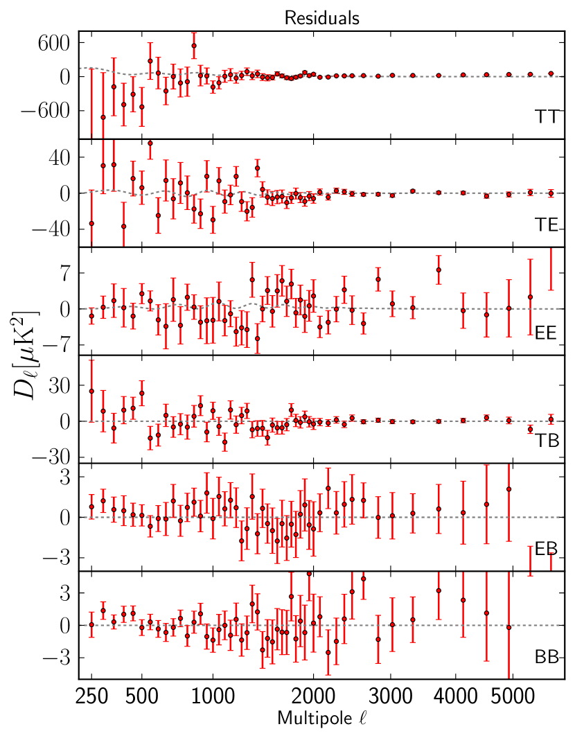
Figure 6.— Residuals of measured power spectra relative to the WMAP+ACT best-fit model (for which TB, EB, and BB are assumed to be zero). Dashed curve shows the small difference between the WMAP+ACT and Planck+WP+highL best-fit models. The $x$-axis is scaled as $\ell^{0.5}$.

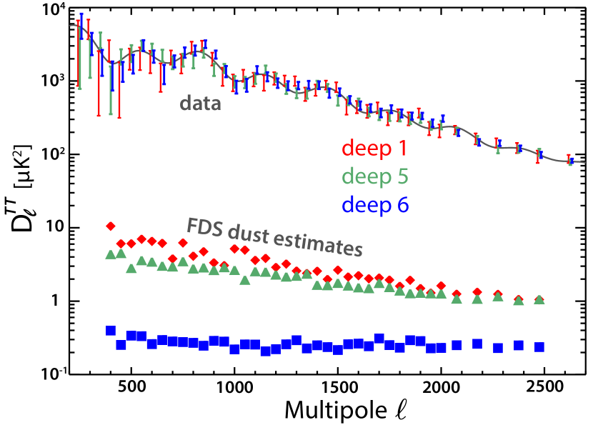
Figure 7.— The expected temperature power spectrum of thermal dust in the ACTPol patches, estimated using the Finkbeiner et al. (1999, FDS) template, plotted below the ACTPol temperature power spectra. The dust amplitude is $\leq 2$ $\mu$K² at $\ell=2000$ ($\sim 1$% of the TT spectrum amplitude, or 10% in the maps). We show that the FDS template is a good tracer of the sub-dominant dust component by correlating it with the ACTPol maps, finding a cross-correlation consistent with unity to within 1$\sigma$.

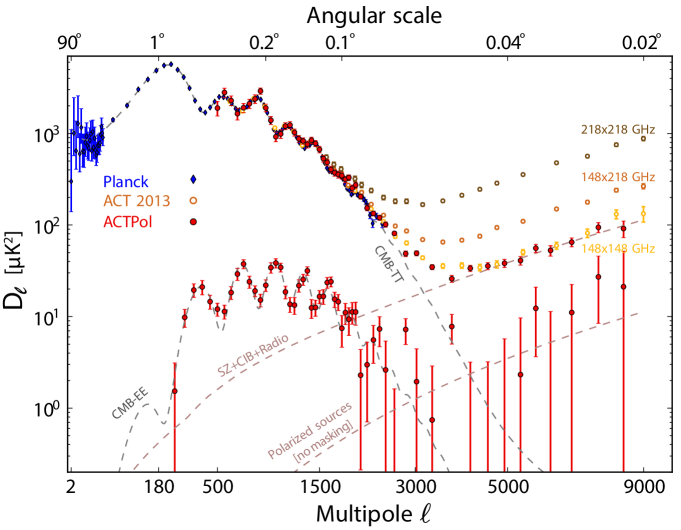
Figure 8.— The Planck, ACT, and ACTPol data. Many Planck points for TT are obscured by the ACT data for $1000<\ell<2500$. The model spectra labeled CMB-TT and CMB-EE are for ‘Planck+WP+highL’ (Planck Collaboration, 2013c). It is clear that the same model is an excellent fit to the TT and EE data (see §4.3.1). Recently WMAP (Bennett et al., 2013) and SPT (Story et al., 2013) have also published new data on the TT spectrum in this range, which are not shown here. All measurements are broadly consistent. The best-fitting Poisson polarized source level is shown, with no sources masked. A non-zero level is preferred, but the distribution is consistent with zero at 95% confidence, with $a_{p}^{\rm pol}<2.4$. The $x$-axis is scaled as $\ell^{0.45}$ to emphasize the mid-$\ell$ range.

4.2. Foreground emission

We test for foreground emission in the temperature maps by correlating the ACTPol maps with the FDS dust template map (Finkbeiner et al., 1999). The dust level in this template has been shown to be consistent with the Planck 353 GHz maps (Planck Collaboration, 2013b) at the $30\%$ level. The predicted contribution of dust to the temperature anisotropy power spectrum is measurable but small, less than $2$ $\mu$K² at $\ell=2000$ as shown in Figure 7. We do not correct for it in the maps or likelihood at this stage.

Based on the recent results from Planck (Planck Collaboration, 2014), the polarization fraction in D1, D5, and D6 is roughly 5%. We take 10% as an upper limit and thus the contribution from polarized dust emission to the power spectrum is expected to be less than $0.02$ $\mu$K² at $\ell=2000$. The contribution from polarized synchrotron emission is expected to be at this level or smaller. A full analysis must await the public release of the Planck polarization maps. However, the consistency shown in Table 1 between patches D1, D5, and D6, each with different foreground levels, suggests that any possible contribution is small compared to the cosmological polarization signal.

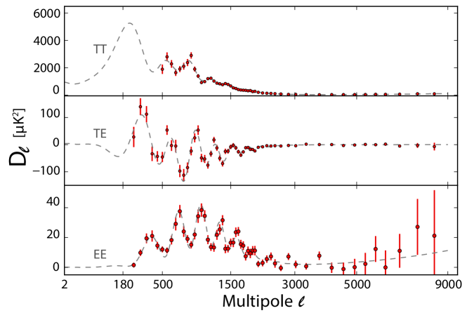
Figure 9.— The ACTPol TT, TE, and EE power spectra, together with the best-fitting $\Lambda$CDM cosmological model and foreground components. Six acoustic peaks are seen in the E-mode polarization, out of phase with the temperature peaks and with the TE correlation pattern predicted by the standard model.

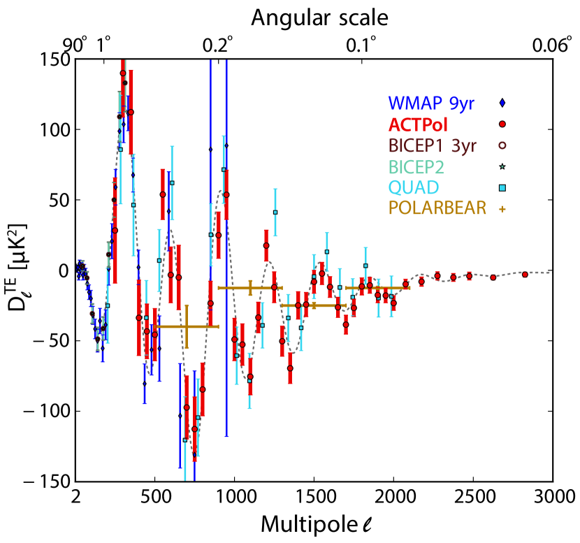
Figure 10.— The ACTPol TE spectrum together with results from WMAP (Bennett et al., 2013), QUAD (QUaD Collaboration, 2009), BICEP1 (BICEP1 Collaboration, 2013), BICEP2 (BICEP2 Collaboration, 2014a), and Polarbear (Polarbear Collaboration, 2014). For ACTPol we correlate with the ACTPol temperature maps, but we could reduce error bars by also correlating with Planck and/or ACT temperature maps. Planck has shown a plot of TE and EE (Figure 11 of Planck Collaboration, 2013c), but the data are not yet available.

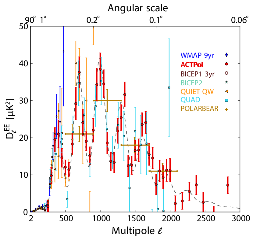
Figure 11.— The ACTPol data together with results from other EE measurements over the past five years, as in Figure 10, and also including QUIET Q and W bands (QUIET Collaboration, 2011, 2012).

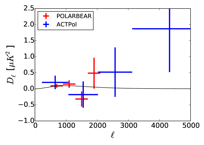
Figure 12.— The ACTPol BB data rebinned into four bins, together with data from (Polarbear Collaboration, 2014). The black curve shows the expected power from lensing B-modes. The ACTPol data points are consistent with zero.

Table 3Rebinned BB power spectrum, ${\cal{D}}_{\ell}=\ell(\ell+1)C_{\ell}/2\pi$ ($\mu$K²), shown in Figure 12.

$\ell$	$\ell$ range	BB
		${\cal{D}}_{\ell}$	$\sigma({\cal{D}}_{\ell})$
650	$225-1075$	0.20	0.21
1550	$1075-2025$	-0.18	0.41
2575	$2025-3125$	0.52	0.77
4325	$3125-5525$	1.87	1.35

4.3. TT,TE,EE,BB

Figure 8 shows the combined ACTPol TT and EE spectra along with independent data sets from ACT temperature measurements and Planck. The full TT/TE/EE set is shown in Figure 9. The TE spectrum is shown in Figure 10, together with results from other CMB polarization experiments. These and the spectra from Figure 6 are presented in Table 6. The bandpowers are not significantly correlated, and bandpower window functions are computed as in Das et al. (2014) to compare theory models to these data. Figure 11 shows the EE spectrum on a linear scale, and Figure 12 shows the BB spectrum rebinned into 4 bins based on the numbers in Table 3. Rebinning to wider bins increases the signal-to-noise ratio at the cost of resolution.

We observe six acoustic peaks in the EE power spectrum, out of phase with the TT spectrum as expected in the standard cosmological model, and six peak/troughs in the TE cross-correlation. We detect no significant BB power.

As a simple test, we find the $\chi^{2}$ for the ACTPol EE data compared to the $\Lambda$CDM 6-parameter model using a) the WMAP+ACT parameters (Calabrese et al., 2013), and b) the Planck best-fit parameters (Planck Collaboration, 2013c). The reduced $\chi^{2}$ values for the two models are 1.09 and 1.12 respectively with 55 dof and no free parameters (with PTE of 0.30 and 0.25). For the TE data the reduced $\chi^{2}$ for the two models are 1.26 and 1.24, again with 55 dof and no free parameters (PTE of 0.09 and 0.18).

Table 4Comparison of cosmological Parameters and 68% confidence intervals for different data sets.

	WMAP+ACT	Planck	ACTPol
			TE,EE
$100\Omega_{b}h^{2}$	$2.247\pm 0.041$	$2.207\pm 0.027$	$2.073\pm 0.135$
$\Omega_{c}h^{2}$	$0.1143\pm 0.0044$	$0.1198\pm 0.0026$	$0.131\pm 0.015$
$10^{4}\theta_{A}$	$103.95\pm 0.19$	$104.132\pm 0.063$	$104.12\pm 0.31$
$\ln(10^{10}A_{s})$	$3.094\pm 0.041$	$3.090\pm 0.025$	$3.190\pm 0.085$
$n_{s}$	$0.970\pm 0.011$	$0.9585\pm 0.0070$	[$0.970\pm 0.011$]
$\tau$	$0.089\pm 0.013$	$0.091\pm 0.0135$	[$0.089\pm 0.013$]
Derived
$\sigma_{8}$	$0.830\pm 0.021$	$0.828\pm 0.012$	$0.933\pm 0.064$
$H_{0}$	$69.7\pm 2.0$	$67.3\pm 1.2$	$63.2\pm 5.5$

4.3.1 $\Lambda$CDM

Another test of the standard $\Lambda$CDM cosmological model is to fit its parameters from just the ACTPol EE and TE data. In this combination, WMAP is used to put a prior on the optical depth and scalar spectral index, since ACTPol does not measure the largest angular scales. We estimate parameters using standard methods as in Sievers et al. (2013) and Calabrese et al. (2013), and marginalize over Poisson source powers for the TE and EE spectra. Other foregrounds are assumed to be unpolarized.

The results are reported in Table 4 and shown in Figure 13 for the physical baryon density, $\Omega_{b}h^{2}$, the physical cold dark matter density, $\Omega_{c}h^{2}$, the acoustic scale $\theta_{A}$, and the amplitude of primordial curvature perturbations, $A_{s}$, defined at pivot scale $k_{0}=0.05$ Mpc^-1. The polarization data are in excellent agreement with the standard model constrained by the Planck temperature data (Planck Collaboration, 2013c).

We repeat the same test with just the ACTPol TT data, including the foreground model as in Dunkley et al. (2013) to account for Poisson and clustered point sources and the thermal and kinematic Sunyaev-Zel’dovich effects. The parameters are consistent with the ACTPol TE/EE results, but more weakly constrain the acoustic scale and the physical baryon and CDM densities (see Figure 13). This highlights the potential of the E-mode polarization signal for cosmological constraints (see e.g., Galli et al., 2014), with sharper acoustic features and less contamination from atmosphere and foregrounds. At this stage of measurement, however, the polarization data are not as precise as the Planck or WMAP temperature data primarily because they are taken over a relatively small region of sky. Parameter constraints from ACTPol combined with Planck are currently dominated by the temperature data.

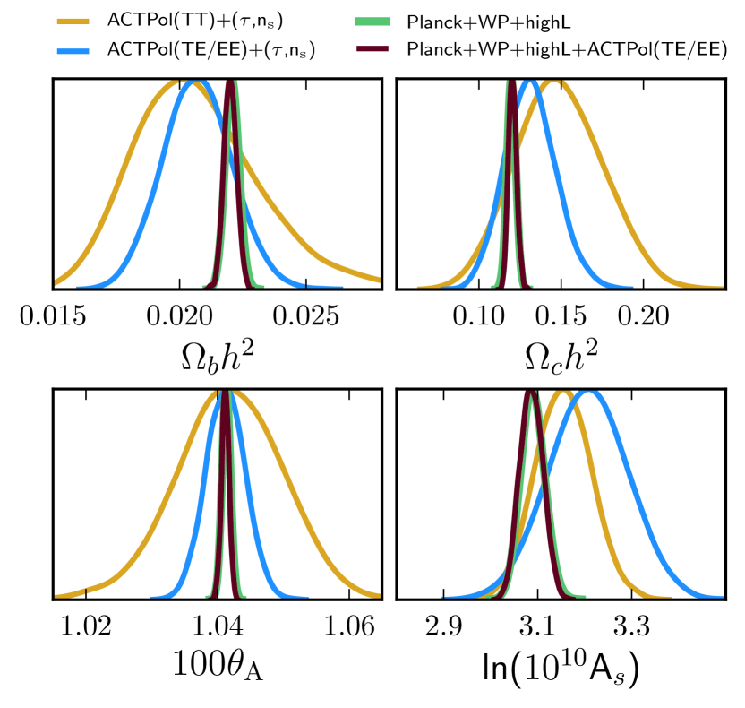
Figure 13.— $\Lambda$CDM parameters estimated from the ACTPol TE and EE data alone(with a prior on the optical depth and spectral index from WMAP), and ACTPol TT alone. They are compared to the constraints from Planck temperature data, and combined Planck and ACTPol TE and EE. The temperature and polarization data give consistent results.

4.3.2 Peak/Dip Phases

$\Lambda$CDM predicts that the TT and polarization peaks should be out of phase. We test this quantitatively, in a manner similar to that used in Readhead et al. (2004). We start by computing the theoretical $\Lambda$CDM TE and EE power spectra based on the best-fit parameters from Section 4.3.1. Since we wish to test for any unexpected phase shift between the TE and EE spectra, we construct a simple parametric model that approximates the $\Lambda$CDM spectra, but has individually adjustable phases for each spectrum. This model takes the form $r_{1}(\ell)+r_{2}(\ell)\cos(2\pi\ell/L+\phi)$ where $r_{1}(\ell)$ and $r_{2}(\ell)$ are rational functions with third-order polynomials in both the numerator and denominator, $L$ is the period of the peaks, and $\phi$ is the phase of the pattern, all of which are fit independently to each spectrum such that the deviation from the $\Lambda$CDM spectra is minimized in the range $100<\ell<2000$. The result is best-fit rational functions $\hat{r}_{1}(\ell)$ and $\hat{r}_{2}(\ell)$ and a best-fit phase parameter $\hat{\phi}$ for each of TT and EE. These modulated rational function models are very good fits to the $\Lambda$CDM spectra, but there is still a small residual. We therefore make the replacement $\hat{r}_{1}(\ell)\rightarrow\hat{r}_{1}(\ell)+\textrm{residual}(\ell)$, such that at $\phi=\hat{\phi}$ the model exactly reproduces the $\Lambda$CDM spectra.

With these models in hand, we are now in the position to ask whether our observed power spectra prefer the same $\phi$ values as $\Lambda$CDM does. For each of TE and EE, we fit linear a three-parameter model $a_{1}\hat{r}_{1}(\ell)+a_{2}\hat{r}_{2}(\ell)\cos(2\pi\ell/L+\hat{\phi})+a_{3}\hat{r}_{2}(\ell)\sin(2\pi\ell/L+\hat{\phi})$ to our observations in the range $225<\ell<2000$. This model effectively encodes a phase shift $\Delta\phi=\phi_{\textrm{data}}-\hat{\phi}={\rm Arg}(a_{2}+ia_{3})$ (our main interest here) as well as a wave amplitude and an overall amplitude factor.

The resulting fits can be seen in Table 5, and are consistent with the $\Lambda$CDM expectations (i.e. the phase shifts are all consistent with zero). A graphical illustration of the fit compared to the prediction and model space can be seen in Figure 14.

Table 5Results of fitting a phase shift in the observed TE and EE spectra relative to the $\Lambda$CDM best-fit model.

	TE	EE	TE+EE
$a_{1}$	$1.036\pm 0.066$	$1.008\pm 0.032$	$1.014\pm 0.032$
$a_{2}$	$1.000\pm 0.080$	$0.985\pm 0.088$	$0.986\pm 0.061$
$a_{3}$	$-0.108\pm 0.080$	$0.108\pm 0.088$	$0.003\pm 0.061$
$\phi_{\textrm{data}}$ (∘)	$23.0$	$-64.9$
$\Delta\phi$ (∘)	$-6.2\pm 4.6$	$6.2\pm 5.1$	$0.2\pm 3.6$

Note: In the last row, a single common phase shift is fit jointly for TE and EE while still using their individual $\phi$ angles. The fits are in agreement with the $\Lambda$CDM expectations.

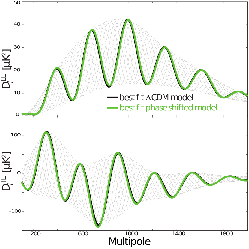
Figure 14.— Recovered amplitudes and phases of the polarization peak/dip pattern from ACTPol data. The black curves mark the best-fit $\Lambda$CDM model power spectrum. The green curves show the best-fit amplitude/phase EE (top) and TE (bottom) models to the ACTPol data as described in the text. The thin lines in the background show the envelope of the phase-shifted model. The polarization data are in excellent agreement with the $\Lambda$CDM prediction.

4.3.3 Polarized point sources

T
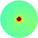
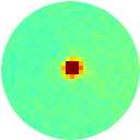
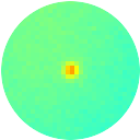
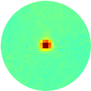
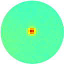
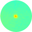
Q
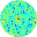
U

Figure 15.— Three of the highest signal-to-noise polarized point sources from each of patch D5 (left) and D6 (right). Each disk has a radius of 8’, with the value range being $\pm 2000\mu$K for T and $\pm 200\mu$K for Q and U. We do not mask polarized sources in this analysis. The sources may be associated with (from left to right) [HB89] 2332-017, [HB89] 2335-027, SDSS J001130.40+005751.7, PKS 0214-085, [HB89] 0226-038 and PKS 0205-010.

We do not detect significantly polarized point sources in the ACTPol maps. Six of the highest signal-to-noise sources found in the D5 and D6 patches are shown in Figure 15; the polarization is barely detectable. For the temperature spectra, point sources above 15 mJy are masked, but no sources exceed this threshold in polarization and none are masked.

We model the Poisson tail of the temperature spectrum as

$${\cal D}_{\ell}=(a_{s}+a_{d})\bigg{(}\frac{\ell}{3000}\bigg{)}^{2}\mu{\rm K}^{2}$$ (2)

(Dunkley et al., 2011), where $a_{s}$ is the amplitude for the residual unmasked radio/synchrotron sources and $a_{d}$ is the amplitude for the pervasive dusty star forming galaxy (DSFG) or CIB component. The latter is unresolved. The two components are separated in ACT temperature measurements with two observing frequencies. In ACTPol we currently have just one frequency and so place a limit on the combined Poisson power: $a_{p}=a_{s}+a_{d}$. In Sievers et al. (2013) we found $a_{s}=3.1\pm 0.4$ and $a_{d}=7.0\pm 0.5$, for a total of $a_{p}=10.3\pm 0.6$ for the TT data. With the ACTPol TT data we find a consistent level of $a_{p}=10.9\pm 1.5$, for the same masking threshold.

Without masking any point sources in the EE data we find $a_{p}^{\rm pol}=1.5\pm 0.6$ at 68% confidence, or $a_{p}^{\rm pol}<2.4$ at 95% confidence. In flux units this corresponds to $C_{\ell}=0.15^{+0.05}_{-0.07}~{}{\rm Jy}^{2}/{\rm sr}$, or $<0.24~{}{\rm Jy}^{2}/{\rm sr}$ (95% CL), at 146 GHz, and puts a limit on all polarized sources before masking.

5. Conclusions

The polarization capabilities of ACTPol have already enabled new probes of the cosmological model. We have shown that ACT is capable of measuring polarization to high accuracy and of measuring CMB temperature and polarization during the day. With one third of the full complement of detectors observing at night over just 90 days, we have already made some of the most competitive measurements yet of CMB polarization at $\ell>1000$. The ACTPol EE, TE, TB, and BB data obtained to date are all in agreement with the standard model of cosmology. We anticipate substantial improvements with more detectors and observing time.

Table 6Combined Power Spectra, ${\cal{D}}_{\ell}=\ell(\ell+1)C_{\ell}/2\pi$ ($\mu$K²), shown in Figures 6 and 9.

$\ell$	$\ell$ range	TT		TE		EE		BB		TB		EB
		${\cal{D}}_{\ell}$	$\sigma({\cal{D}}_{\ell})$	${\cal{D}}_{\ell}$	$\sigma({\cal{D}}_{\ell})$	${\cal{D}}_{\ell}$	$\sigma({\cal{D}}_{\ell})$	${\cal{D}}_{\ell}$	$\sigma({\cal{D}}_{\ell})$	${\cal{D}}_{\ell}$	$\sigma({\cal{D}}_{\ell})$	${\cal{D}}_{\ell}$	$\sigma({\cal{D}}_{\ell})$
250	$225-275$	4049.4	1476.4	28.3	37.3	1.5	1.6	0.1	1.2	25.1	25.9	0.8	0.9
300	$275-325$	3366.7	788.5	139.9	31.2	9.8	2.2	1.4	0.8	8.5	17.3	1.2	0.9
350	$325-375$	2377.3	510.0	112.2	29.7	19.5	3.3	0.3	0.7	-5.7	12.4	0.6	0.9
400	$375-425$	1366.2	376.3	-33.7	26.8	21.0	3.8	1.0	0.7	9.3	11.4	0.5	1.1
450	$425-475$	1683.2	310.0	-43.3	19.4	14.6	2.5	1.1	0.7	10.9	9.2	0.2	0.9
500	$475-525$	1892.9	342.9	-45.6	18.5	12.1	2.0	-0.2	0.7	23.4	10.4	0.1	0.8
550	$525-575$	2801.0	323.5	53.8	17.8	11.4	2.0	0.3	0.7	-14.1	9.8	-0.7	0.8
600	$575-625$	2284.9	278.6	-3.3	19.8	18.3	3.0	-0.3	0.8	-11.5	9.1	-0.1	1.0
650	$625-675$	1644.6	242.7	-5.1	22.8	29.2	4.4	-0.7	0.8	4.9	9.3	-0.1	1.2
700	$675-725$	1907.0	218.9	-97.3	22.4	37.6	4.2	-0.2	0.8	-4.8	8.6	1.2	1.2
750	$725-775$	2112.9	246.5	-112.6	22.8	24.0	3.6	0.6	0.8	-2.4	8.8	-0.3	1.1
800	$775-825$	2381.3	257.2	-84.5	18.7	19.1	2.5	-1.0	1.0	-4.9	10.0	0.7	1.0
850	$825-875$	2904.4	228.6	-23.5	15.7	15.2	2.4	0.3	1.0	4.2	9.1	1.1	1.0
900	$875-925$	1901.5	181.3	24.9	16.4	22.0	3.2	1.1	1.0	13.0	8.3	0.1	1.2
950	$925-975$	1393.4	140.3	53.6	17.4	34.3	4.5	-1.0	1.2	-9.0	8.2	1.8	1.5
1000	$975-1025$	920.8	109.2	-49.0	15.0	38.4	4.5	-1.4	1.1	8.8	7.1	-0.1	1.5
1050	$1025-1075$	987.4	107.8	-52.7	14.7	34.5	3.8	-0.4	1.4	-4.3	7.5	1.5	1.4
1100	$1075-1125$	1203.5	105.2	-75.5	12.9	18.6	3.0	-0.0	1.3	-17.4	7.6	0.6	1.3
1150	$1125-1175$	1234.2	107.1	-33.5	10.9	13.6	2.5	-0.9	1.4	9.4	7.6	1.3	1.3
1200	$1175-1225$	1026.2	90.6	17.6	10.9	13.3	2.8	0.6	1.5	-2.8	7.2	0.7	1.5
1250	$1225-1275$	875.3	74.9	-12.0	10.9	21.8	3.3	-1.4	1.5	4.8	6.9	-1.8	1.5
1300	$1275-1325$	828.4	65.6	-50.3	10.7	25.4	3.5	-0.7	1.5	8.6	6.3	-0.8	1.5
1350	$1325-1375$	761.1	67.4	-69.5	10.9	31.6	3.4	2.0	1.7	-7.0	6.8	1.5	1.7
1400	$1375-1425$	843.5	66.0	-24.9	9.7	12.5	2.9	1.2	1.7	-6.0	6.5	-1.2	1.5
1450	$1425-1475$	778.9	60.2	-24.3	8.5	12.6	2.5	-2.3	1.7	-5.9	6.6	0.7	1.4
1500	$1475-1525$	668.3	54.3	-8.1	8.1	16.5	2.7	-1.2	1.7	-13.7	6.2	-0.5	1.5
1550	$1525-1575$	530.9	42.9	-2.3	7.9	16.6	3.1	-1.5	2.0	-3.2	5.8	-1.0	1.7
1600	$1575-1625$	482.7	37.1	-11.8	7.3	23.5	3.2	-0.4	1.9	-5.5	5.3	-1.8	1.7
1650	$1625-1675$	404.7	33.2	-26.2	7.2	24.1	3.0	-0.6	2.1	-5.5	5.2	-0.5	1.7
1700	$1675-1725$	372.8	31.6	-38.5	6.6	15.5	2.9	-0.7	2.0	-2.8	5.1	-1.5	1.7
1750	$1725-1775$	356.3	31.0	-26.7	6.2	14.5	2.9	2.7	2.3	9.3	5.4	-0.5	1.7
1800	$1775-1825$	346.6	28.8	-11.4	6.1	7.5	2.8	-1.3	2.2	0.7	5.1	-1.3	1.7
1850	$1825-1875$	315.5	24.4	-10.6	5.6	11.1	2.9	0.4	2.4	-0.9	4.7	0.2	1.8
1900	$1875-1925$	330.0	22.2	-17.6	5.4	9.4	3.1	-0.7	2.5	3.8	4.7	0.9	1.9
1950	$1925-1975$	252.6	20.4	-17.9	5.1	11.2	3.0	4.8	2.5	-0.4	4.4	-0.6	1.8
2000	$1975-2025$	272.6	19.1	-23.2	5.2	11.2	3.2	0.2	2.7	-2.3	4.6	-0.9	2.0
2075	$2025-2125$	204.5	12.5	-9.8	3.5	2.3	2.1	0.8	1.9	-0.7	3.1	0.3	1.4
2175	$2125-2225$	153.2	10.3	-8.0	3.3	3.0	2.3	-2.5	2.1	-1.5	2.9	2.1	1.5
2275	$2225-2325$	133.9	8.3	-3.9	2.9	5.6	2.5	-1.5	2.2	1.1	2.8	0.3	1.6
2375	$2325-2425$	120.1	7.4	-5.1	2.9	7.3	2.6	0.6	2.3	-2.6	2.7	1.0	1.7
2475	$2425-2525$	101.4	6.7	-4.0	2.8	2.6	2.8	3.1	2.5	2.7	2.6	1.3	1.8
2625	$2525-2725$	81.1	4.1	-5.1	1.8	-0.4	2.1	4.3	1.9	-0.4	1.7	1.3	1.3
2825	$2725-2925$	48.6	3.5	-3.0	1.8	7.2	2.3	-1.3	2.2	0.9	1.7	-0.0	1.5
3025	$2925-3125$	49.2	3.1	-4.0	1.8	1.9	2.5	0.1	2.5	-0.3	1.7	0.1	1.7
3325	$3125-3525$	34.7	2.2	1.7	1.3	0.7	2.1	0.5	2.1	-0.5	1.3	0.3	1.5
3725	$3525-3925$	25.9	2.3	0.3	1.6	7.8	2.8	3.2	2.7	-0.1	1.5	0.6	1.8
4125	$3925-4325$	33.7	2.6	0.2	1.8	-0.3	3.4	2.3	3.4	0.6	1.8	0.3	2.3
4525	$4325-4725$	35.7	3.2	-3.3	2.3	-1.1	4.3	1.1	4.5	3.0	2.3	1.0	2.9
4925	$4725-5125$	38.2	3.9	-1.4	2.9	0.1	5.6	-0.2	5.6	0.7	2.8	2.1	3.9
5325	$5125-5525$	40.9	4.5	0.8	3.5	2.3	7.4	11.7	7.1	-6.7	3.5	-7.0	4.9
5725	$5525-5925$	55.8	5.7	-0.2	4.3	12.3	8.7	24.4	8.9	1.6	4.2	-8.7	6.0
6125	$5925-6325$	52.7	6.9	1.8	5.6	-0.0	11.4	2.6	11.2	-0.5	5.3	1.5	7.7
6725	$6325-7125$	65.0	7.2	-5.1	5.3	11.1	11.3	12.6	11.3	4.0	5.4	11.9	7.7
7525	$7125-7925$	94.3	12.0	-3.0	8.7	27.1	18.7	43.0	17.9	-2.9	8.6	25.5	12.7
8325	$7925-8725$	91.6	18.7	-7.0	14.0	21.2	30.6	18.6	30.3	14.4	14.0	14.1	20.8

References

- Ade et al. (2006) Ade, P. A. R., Pisano, G., Tucker, C., & Weaver, S. 2006, in Society of Photo-Optical Instrumentation Engineers (SPIE) Conference Series, Vol. 6275
- Alexander et al. (2009) Alexander, S., Ochoa, J., & Kosowsky, A. 2009, arXiv:0810.2355, Phys. Rev. D, 79, 063524
- Anderson et al. (2014) Anderson, L., et al. 2014, arXiv:1312.4877, MNRAS, 441, 24
- Arendt et al. (2011) Arendt, R. G., et al. 2011, arXiv:1103.6225, ApJ, 734, 54
- Aumont et al. (2010) Aumont, J., et al. 2010, A&A, 514, A70
- Battistelli et al. (2008) Battistelli, E. S., et al. 2008, in Society of Photo-Optical Instrumentation Engineers (SPIE) Conference Series, Vol. 7020
- Becker et al. (1995) Becker, R. H., White, R. L., & Helfand, D. J. 1995, ApJ, 450, 559
- Bennett et al. (2011) Bennett, C. L., et al. 2011, arXiv:1001.4758, ApJS, 192, 17
- Bennett et al. (2013) —. 2013, arXiv:1212.5225, ApJS, 208, 20
- Betoule et al. (2014) Betoule, M., et al. 2014, arXiv:1401.4064, A&A, 568, A22
- BICEP1 Collaboration (2013) BICEP1 Collaboration. 2013, arXiv:1310.1422
- BICEP2 Collaboration (2014a) BICEP2 Collaboration. 2014a, arXiv:1403.3985
- BICEP2 Collaboration (2014b) —. 2014b, arXiv:1403.4302
- Bond & Efstathiou (1987) Bond, J. R. & Efstathiou, G. 1987, MNRAS, 226, 655
- BOSS (2014) BOSS. 2014, http://www.sdss3.org/surveys/boss.php
- Britton et al. (2010) Britton, J. W., et al. 2010, arXiv:1007.0805, in Society of Photo-Optical Instrumentation Engineers (SPIE) Conference Series, Vol. 7741
- Bucher et al. (2004) Bucher, M., Dunkley, J., Ferreira, P. G., Moodley, K., & Skordis, C. 2004, astro-ph/0401417, Physical Review Letters, 93, 081301
- Calabrese et al. (2013) Calabrese, E., et al. 2013, arXiv:1302.1841, Phys. Rev. D, 87, 103012
- Calabrese et al. (2014) —. 2014, arXiv:1406.4794, J. Cosmology Astropart. Phys, 8, 10
- CAPMAP Collaboration (2008) CAPMAP Collaboration. 2008, arXiv:0802.0888, ApJ, 684, 771
- CFHTLens Collaboration (2013) CFHTLens Collaboration. 2013, arXiv:1210.8156, MNRAS, 433, 2545
- Chervenak et al. (1999) Chervenak, J. A., Irwin, K. D., Grossman, E. N., Martinis, J. M., Reintsema, C. D., & Huber, M. E. 1999, Applied Physics Letters, 74, 4043
- Cooray et al. (2003) Cooray, A., Melchiorri, A., & Silk, J. 2003, astro-ph/0205214, Physics Letters B, 554, 1
- Copi et al. (2010) Copi, C. J., Huterer, D., Schwarz, D. J., & Starkman, G. D. 2010, arXiv:1004.5602, Advances in Astronomy, 2010
- Das et al. (2011) Das, S., et al. 2011, arXiv:1009.0847, ApJ, 729, 62
- Das et al. (2014) —. 2014, arXiv:1301.1037, J. Cosmology Astropart. Phys, 4, 14
- Datta et al. (2013) Datta, R., et al. 2013, arXiv:1307.4715, Appl. Opt., 52, 8747
- Datta et al. (2014) —. 2014, arXiv:1401.8029, Journal of Low Temperature Physics, Feb. 2014
- de Jong et al. (2013) de Jong, J. T. A., Verdoes Kleijn, G. A., Kuijken, K. H., & Valentijn, E. A. 2013, arXiv:1206.1254, Experimental Astronomy, 35, 25
- DES (2014) DES. 2014, https://www.darkenergysurvey.org/index.shtml
- Dicke (1946) Dicke, R. H. 1946, Review of Scientific Instruments, 17, 268
- Driver et al. (2009) Driver, S. P., et al. 2009, arXiv:0910.5123, Astronomy and Geophysics, 50, 050000
- Dunkley et al. (2011) Dunkley, J., et al. 2011, arXiv:1009.0866, ApJ, 739, 52
- Dunkley et al. (2013) —. 2013, arXiv:1301.0776, J. Cosmology Astropart. Phys, 7, 25
- Dünner et al. (2013) Dünner, R., et al. 2013, arXiv:1208.0050, ApJ, 762, 10
- Durret et al. (2011) Durret, F., et al. 2011, arXiv:1109.0850, A&A, 535, A65
- Finkbeiner et al. (1999) Finkbeiner, D. P., Davis, M., & Schlegel, D. J. 1999, astro-ph/9905128, ApJ, 524, 867
- Fowler et al. (2007) Fowler, J. W., et al. 2007, astro-ph/0701020, Appl. Opt., 46, 3444
- Galli et al. (2014) Galli, S., et al. 2014, arXiv:1403.5271
- Garilli et al. (2014) Garilli, B., et al. 2014, arXiv:1310.1008, A&A, 562, A23
- Górski et al. (2005) Górski, K. M., Hivon, E., Banday, A. J., Wandelt, B. D., Hansen, F. K., Reinecke, M., & Bartelmann, M. 2005, astro-ph/0409513, ApJ, 622, 759
- Grace et al. (2014) Grace, E., et al. 2014, ACTPol: on-sky performance and characterization
- Grace et al. (2014) Grace, E. A., et al. 2014, Journal of Low Temperature Physics
- Güsten et al. (2006) Güsten, R., Nyman, L. Å., Schilke, P., Menten, K., Cesarsky, C., & Booth, R. 2006, A&A, 454, L13
- Hamaker & Bregman (1996) Hamaker, J. P. & Bregman, J. D. 1996, A&AS, 117, 161
- Hanson et al. (2013) Hanson, D., et al. 2013, arXiv:1307.5830, Physical Review Letters, 111, 141301
- Hasselfield et al. (2013) Hasselfield, M., et al. 2013, arXiv:1303.4714, ApJS, 209, 17
- Hester (2008) Hester, J. J. 2008, ARA&A, 46, 127
- Hincks et al. (2010) Hincks, A. D., et al. 2010, arXiv:0907.0461, ApJS, 191, 423
- Hinshaw et al. (2013) Hinshaw, G., et al. 2013, arXiv:1212.5226, ApJS, 208, 19
- Hou et al. (2014) Hou, Z., et al. 2014, arXiv:1212.6267, ApJ, 782, 74
- Hubmayr et al. (2012) Hubmayr, J., et al. 2012, Journal of Low Temperature Physics, 167, 904
- Jeong et al. (2014) Jeong, D., Chluba, J., Dai, L., Kamionkowski, M., & Wang, X. 2014, arXiv:1309.2285, Phys. Rev. D, 89, 023003
- Kamionkowski et al. (1997) Kamionkowski, M., Kosowsky, A., & Stebbins, A. 1997, astro-ph/9609132, Physical Review Letters, 78, 2058
- Keating et al. (2013) Keating, B. G., Shimon, M., & Yadav, A. P. S. 2013, arXiv:1211.5734, ApJ, 762, L23
- Kosowsky et al. (2005) Kosowsky, A., Kahniashvili, T., Lavrelashvili, G., & Ratra, B. 2005, astro-ph/0409767, Phys. Rev. D, 71, 043006
- Louis et al. (2013) Louis, T., Næss, S., Das, S., Dunkley, J., & Sherwin, B. 2013, arXiv:1306.6692, MNRAS, 435, 2040
- Louis et al. (2014) Louis, T., et al. 2014, arXiv:1403.0608
- Lue et al. (1999) Lue, A., Wang, L., & Kamionkowski, M. 1999, astro-ph/9812088, Physical Review Letters, 83, 1506
- Macías-Pérez et al. (2010) Macías-Pérez, J. F., Mayet, F., Aumont, J., & Désert, F.-X. 2010, arXiv:0802.0412, ApJ, 711, 417
- MacTavish et al. (2006) MacTavish, C. J., et al. 2006, astro-ph/0507503, ApJ, 647, 799
- Manzotti et al. (2014) Manzotti, A., Hu, W., & Benoit-Lévy, A. 2014, arXiv:1401.7992
- Næss & Louis (2013) Næss, S. & Louis, T. 2013, arXiv:1309.7473
- Niemack et al. (2010) Niemack, M. D., et al. 2010, arXiv:1006.5049, in Society of Photo-Optical Instrumentation Engineers (SPIE) Conference Series, Vol. 7741
- Oliver et al. (2012) Oliver, S. J., et al. 2012, arXiv:1203.2562, MNRAS, 424, 1614
- Pappas et al. (2014) Pappas, C. G., et al. 2014, Journal of Low Temperature Physics
- Planck Collaboration (2013a) Planck Collaboration. 2013a, arXiv:1303.5062
- Planck Collaboration (2013b) —. 2013b, arXiv:1312.1300
- Planck Collaboration (2013c) —. 2013c, arXiv:1303.5076
- Planck Collaboration (2013d) —. 2013d, arXiv:1303.5083
- Planck Collaboration (2014) —. 2014, arXiv:1405.0871
- QUaD Collaboration (2009) QUaD Collaboration. 2009, arXiv:0906.1003, ApJ, 705, 978
- QUIET Collaboration (2011) QUIET Collaboration. 2011, arXiv:1012.3191, ApJ, 741, 111
- QUIET Collaboration (2012) —. 2012, arXiv:1207.5034, ApJ, 760, 145
- Readhead et al. (2004) Readhead, A. C. S., et al. 2004, astro-ph/0409569, Science, 306, 836
- Rocha et al. (2004) Rocha, G., Trotta, R., Martins, C. J. A. P., Melchiorri, A., Avelino, P. P., Bean, R., & Viana, P. T. P. 2004, astro-ph/0309211, MNRAS, 352, 20
- SDSS (2014) SDSS. 2014, http://www.sdss.org
- Shimon et al. (2008) Shimon, M., Keating, B., Ponthieu, N., & Hivon, E. 2008, arXiv:0709.1513, Phys. Rev. D, 77, 083003
- Sievers et al. (2007) Sievers, J. L., et al. 2007, astro-ph/0509203, ApJ, 660, 976
- Sievers et al. (2013) —. 2013, arXiv:1301.0824, J. Cosmology Astropart. Phys, 10, 60
- Spergel et al. (2003) Spergel, D. N., et al. 2003, astro-ph/0302209, ApJS, 148, 175
- Story et al. (2013) Story, K. T., et al. 2013, arXiv:1210.7231, ApJ, 779, 86
- Subaru (2014) Subaru. 2014, http://www.naoj.org/Projects/HSC/
- Suzuki et al. (2012) Suzuki, N., et al. 2012, arXiv:1105.3470, ApJ, 746, 85
- Swetz et al. (2011) Swetz, D. S., et al. 2011, arXiv:1007.0290, ApJS, 194, 41
- Polarbear Collaboration (2013) Polarbear Collaboration. 2013, arXiv:1312.6645
- Polarbear Collaboration (2014) —. 2014, arXiv:1403.2369
- Tucker & Ade (2006) Tucker, C. E. & Ade, P. A. R. 2006, in Society of Photo-Optical Instrumentation Engineers (SPIE) Conference Series, Vol. 6275
- Véron-Cetty & Véron (2006) Véron-Cetty, M.-P. & Véron, P. 2006, A&A, 455, 773
- Viero et al. (2014) Viero, M. P., et al. 2014, arXiv:1308.4399, ApJS, 210, 22
- Weiland et al. (2011) Weiland, J. L., et al. 2011, arXiv:1001.4731, ApJS, 192, 19
- White et al. (1997) White, R. L., Becker, R. H., Helfand, D. J., & Gregg, M. D. 1997, VizieR Online Data Catalog, 8048, 0
- XMM-XXL (2014) XMM-XXL. 2014, http://sci.esa.int/xmm-newton/48357-xxl-the-ultimate-xmm-extragalactic-survey/
- Zaldarriaga & Seljak (1997) Zaldarriaga, M. & Seljak, U. 1997, astro-ph/9609170, Phys. Rev. D, 55, 1830
- Zaldarriaga & Seljak (1998) —. 1998, astro-ph/9803150, Phys. Rev. D, 58, 023003