Classical kinematics and Finsler structures for nonminimal Lorentz-violating fermions
Abstract
In the current paper the Lagrangian of a classical, relativistic point particle is obtained whose conjugate momentum satisfies the dispersion relation of a quantum wave packet that is subject to Lorentz violation based on a particular coefficient of the nonminimal Standard-Model Extension (SME). The properties of this Lagrangian are analyzed and two corresponding Finsler structures are obtained. One structure describes a scaled Euclidean geometry, whereas the other is neither a Riemann nor a Randers or Kropina structure. The results of the article provide some initial understanding of classical Lagrangians of the nonminimal SME fermion sector.
pacs:
11.30.Cp, 14.60.Cd, 45.20.Jj, 02.40.-kI Introduction
Finsler’s interests as a Ph.D. student rested upon geometries characterized by path length functionals that were generalized versions of the Riemannian definition. He studied manifolds whose geometric properties such as curvature both depend on the point considered on the manifold and on the angle that a chosen line element encloses with a given direction in the tangent space of the manifold Finsler:1918 . Subsequently these types of spaces were called Finsler spaces by Cartan Cartan:1933 ; Cartan:1934 . According to Chern Chern:1996 it should be avoided saying that Finsler spaces are a generalization of Riemannian ones. Instead, it is better to denote them as Riemannian spaces without the quadratic restriction.
The monographs Antonelli:1993 ; Bao:2000 deliver a mathematical introduction of Finsler geometry including various applications. A Finsler space is, indeed, not a point space but a set of line elements. Each is endowed with an underlying Riemannian metric Busemann:1950 , which determines vector magnitudes and angles between vectors. Besides, a real-valued function on its tangent bundle is introduced, which has certain properties and is often denoted as a Finsler structure. One basic example for a Finsler structure is provided by the time that a salesman needs to travel between different locations on a hillside (see p. 46 in Antonelli:1993 , Kozma:2003 ). The solution of the Zermelo navigation problem, which asks the question of minimizing the navigation time of a ship or plane in the presence of wind, leads to a further example of a Finsler structure.
One essential application of Finsler geometry lies in the field of Lorentz symmetry violation, which was initiated by the seminal articles Kostelecky:1988zi ; Kostelecky:1991ak ; Kostelecky:1994rn ; oai:arXiv.org:hep-th/9605088 . Since the development of the (minimal) Standard-Model Extension (SME) Colladay:1998fq the investigation of Lorentz violation has become more and more prominent. The (minimal) SME is a framework of all power-counting renormalizable, Lorentz-violating operators compatible with the Standard Model of elementary particle physics. The minimal SME was extended by the nonminimal SME Kostelecky:2009zp ; Kostelecky:2011gq ; Kostelecky:2013rta , which comprises all Lorentz-violating terms having arbitrary operator dimension.
In this context the interest lies in establishing a correspondence between the dispersion relation of a quantum wave packet, which follows from the Lorentz-violating field theory, and the kinematics of a classical, relativistic point particle. So the goal is to associate classical Lagrangians to the SME and there are several good reasons for doing that. First, the latter may be closely linked to a Finsler space, which has already been thoroughly investigated by mathematicians. This will provide a large toolbox of methods and theorems to understand the classical limit of the SME in an elegant way. Second, the dispersion relation is merely a first integral of the equations of motion. The motion of a particle in a background field can only be completely analyzed once the equations of motion are known. Third, Finsler geometry is a reasonable and natural procedure to describe background fields in a (curved) manifold, e.g., Lorentz violation in the presence of gravity. This can be done by promoting the constant Lorentz-violating coefficients to spacetime-dependent functions and by replacing the flat intrinsic metric with a curved metric.
Before delving into the physics, a classical Lagrangian in flat spacetime has to be found and its properties must be understood. In Kostelecky:2010hs ; Colladay:2012rv ; Russell:2015gwa classical Lagrangians were derived for certain sets of Lorentz-violating coefficients of the minimal SME fermion sector. In Kostelecky:2011qz ; Colladay:2012rv ; Kostelecky:2012ac these Lagrangians were promoted to Finsler structures, which were then inspected closely. The goal of the current paper is to carry this out for a framework based on a particular Lorentz-violating coefficient of the nonminimal fermion sector. The properties of this Lagrangian will be investigated with the result that it can be promoted to two different Finsler structures.
In general, a playground for Finsler geometry in physics is investigating modifications of relativity. One of the first applications was delivered by Randers in Randers:1940 . The Finsler structure introduced by him carries his name and is of great importance in science. For example, the structure being a solution of the Zermelo navigation problem is of Randers type. Questions of spacetime causality in relation to Finsler structures were addressed in Caponio:2007dt ; Caponio:2009er where Randers structures play an essential role as well. In Russell:2014 a Randers structure is used to determine speed limits in quantum information processing.
Further applications of Finsler geometry include but are not restricted to optical geometry and gravitational lensing in general relativity Gibbons:2008zi ; Caponio:2011dm ; Werner:2012rc , geometrical optics in anisotropic media Skakala:2008jp , electron optics under the influence of magnetic fields, thermodynamics, biology (see Antonelli:1993 for the latter topics), psychometry Kozma:2003 , dynamical systems Kawaguchi:1977 ; Bucataru:2007 , and imaging Astola:2010 .
Note that Finsler spacetimes have recently been examined in the literature more profoundly. Due to their pseudo-Riemannian signature, the definition of Finsler spacetimes is more involved than that of Finsler geometries with a Riemannian signature. In Pfeifer:2011tk ; Pfeifer:2012mb ; Pfeifer:2011xi ; Pfeifer:2011ve ; Hohmann:2013fca Finsler spacetimes are constructed such that they have a light cone structure and allow for the notion of timelike and lightlike vectors. Implications of a Finsler spacetime geometry on a scalar quantum field theory were investigated in Brandt:1998cw ; Brandt:2000ph and references therein. The concept of Finsler spacetimes is also applied, e.g., in the context of very special relativity Zhang:2012hi . In Perlick:2005hz ; Torrome:2012kt ; Torrome:2013rt ; Javaloyes:2013ika Finsler spaces and spacetimes are investigated further. In the first and second of these articles the analogue of Fermat’s principle in special Finsler spacetimes is analyzed. Reference Torrome:2013rt deals with the geodesic deviation equation and applies the obtained results in the context of gravity. The paper Javaloyes:2013ika reviews causality in Finsler spacetimes and the correspondence between standard stationary spacetimes and Randers spaces. In a certain sense, Finsler spacetimes generalize Lorentz invariance instead of violating it Pfeifer:2011ve .
The paper is organized as follows. Sections II, III give brief introductions to the nonminimal SME fermion sector and describe how to obtain the classical point-particle Lagrangian from the fermion dispersion relation. In Sec. IV the classical Lagrangian is derived for the sector considered and its characteristics are investigated. Section V briefly reviews the mathematics of Finsler structures and demonstrates how such structures can be obtained from the classical Lagrangian computed. Finally in Sec. VI the physics of the Lagrangian is discussed assuming a sufficiently small Lorentz-violating coefficient. Last but not least the results of the paper are summarized in Sec. VII. Calculational details are relegated to the appendix and natural units with are used throughout the article.
II Fermion sector of the nonminimal Standard-Model Extension
The SME is a collection of all Lorentz-violating operators of Standard Model fields that are gauge-invariant with respect to . The minimal sector comprises power-counting renormalizable terms, whereas the nonminimal sector includes all contributions up to arbitrary operator dimension. In Kostelecky:2013rta the operators of the nonminimal SME fermion sector are classified according to their transformation properties under the improper Lorentz transformations P, T and charge conjugation C. The action of the nonminimal Lorentz-violating fermion sector reads
| (2.1) |
Here is the standard Dirac field, the Dirac conjugate field, is the fermion mass, and the unit matrix in spinor space. The gamma matrices for are standard and satisfy the Clifford algebra with the flat Minkowski metric with signature . The quantity comprises any possible Lorentz-violating operator of the fermion sector.
In the recent article Schreck:2014qka certain quantum field theoretic properties of some families of nonminimal operators were investigated. One of the sets of coefficients studied was the dimension-5 part of the Lorentz scalar , i.e., . These coefficients are CPT-even and supposedly the simplest of higher dimension. We consider an observer frame where all coefficients vanish except of . Then the theory to be examined is characterized by the action of Eq. (2.1) with . The modified off-shell dispersion law reads
| (2.2) |
which is quartic in . The coefficient has mass dimension , which gives the product the suitable mass dimension 1, such that it can be added to the fermion mass . The solutions of Eq. (2.2) with respect to are the modified dispersion relations of an on-shell fermion affected by the single coefficient . There are two dispersion relations that are perturbed versions of the standard dispersion law with the spatial momentum . These are stated in Schreck:2014qka . Besides, there are two spurious dispersion laws that do not correspond to the standard limit for a vanishing Lorentz-violating coefficient.
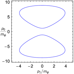
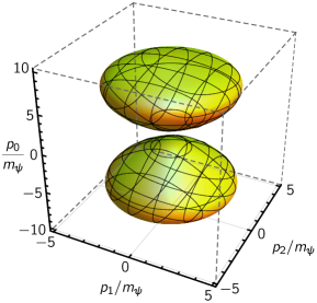
Two- and three-dimensional slices of the dispersion law given in Eq. (2.2) are plotted in Fig. 1 for a particular Lorentz-violating coefficient . In comparison to the standard fermion dispersion relation the resulting surface is not a two-shell hyperboloid, but it is homeomorphic to two disconnected (hyper)spheres. For momenta lying in the order of magnitude of the dispersion relation is heavily modified, which even changes the topology of the corresponding (hyper)surface. Because of this there are regions with vertical tangents on the (hyper)surface corresponding to infinite group velocities.
These properties are characteristic for frameworks based on Lorentz-violating operators involving additional time derivatives. Even for minimal operators additional time derivatives lead to an unconventional time evolution of states, which is why asymptotic states do not correspond to physical free-particle states directly Colladay:2001wk . The spurious modes can be understood as Planck-scale effects and for kinematics they do not play a role as long as the particle energy and momentum are much smaller than the Planck scale where the SME is valid as an effective framework. In Schreck:2014qka it was demonstrated that the spurious modes for the dimension-5 operator involving do not lead to problems with unitarity. Therefore the particular dispersion relation of Eq. (2.2) results in a consistent quantum field theory (at least at tree-level), which is why it will be taken as a basis for this article.
The SME is suitable to describe the sub-Planckian limit of an underlying, fundamental theory — howsoever the latter may look like. Even if at the level of effective field theory certain issues arise for energies in the vicinity of the Planck scale such as infinite group velocities, they are expected to be cured by other Lorentz-violating operators stepping in. After all, the underlying theory should be well-behaved right up to the Planck scale.
III Obtaining classical Lagrangians from dispersion relations
In general, the field equations of the SME lead to modified particle dispersion relations with the particle energy and the spatial momentum components ; see, for example, Eq. (2.2) for the nonminimal fermion sector considered. The dispersion relations are necessary conditions for the free-field equations to have nontrivial plane wave solutions. By introducing appropriate smearing functions these plane waves can be used to construct quantum wave packets.
Given a dispersion relation , which is modified by a Lorentz-violating background field, a Finsler structure can be constructed as follows. Consider a classical, relativistic point particle at the spacetime point with a four-velocity () whose kinematics is described by a Lagrangian . The goal is to find a Lagrangian such that its canonical momentum obeys the dispersion relation of the quantum wave packet. Hence one looks for a correspondence between the dispersion relation, which is a quantum field theoretic result, and the Lagrangian of a classical point particle. Note that contrary to most other contexts in field theory the canonical momentum is defined with a minus sign to ensure the kinetic energy in the nonrelativistic limit to be nonnegative.
The classical point particle travels along a well-defined trajectory. All physical results, especially the action, should not depend on the choice of its parameterization. This is granted as long as is positively homogeneous of degree 1 in :
| (3.1) |
Since the Lagrangian has this property, according to a theorem by Euler Bao:2000 it can be written as follows:
| (3.2) |
The latter equation is very helpful. If the momentum can be determined as a function of the velocity, it leads us to the Lagrangian immediately.
For most purposes the group velocity of a quantum wave packet can be interpreted as its physical velocity. To establish the correspondence to the classical point particle, the spatial velocity components of the point particle shall correspond to the group velocity components of the wave packet:
| (3.3) |
The off-shell dispersion relation (for example, Eq. (2.2)) and Eqs. (3.2), (3.3) give five equations of the nine unknowns , , and . Four of these equations must be used to eliminate in favor of and . The procedure employed in most cases considered in the literature so far was to use to eliminate , which then led to a polynomial of . The classical Lagrangian is given by one of the zeros of the latter polynomial with respect to . In the next section it will become evident that a different procedure will lead to the goal here.
IV Classical Lagrangian
Now the interest lies in the Lagrangian for a classical point particle reproducing the dispersion relation of a spin-1/2 fermion underlying Lorentz violation with the single nonzero coefficient given by Eq. (2.2). According to Sec. III the group velocity of a quantum-mechanical wave packet ought to be equal to the three-velocity of the corresponding point particle. The group velocity components can be obtained by implicit differentiation of Eq. (2.2) and solving the resulting equation with respect to . This leads to
| (4.1) |
Using Eq. (4.1) the spatial momentum components can be expressed via . Inserting these relations in the off-shell dispersion relation of Eq. (2.2), the resulting equation can be solved with respect to . Calculational details of this procedure are outlined in App. A. The computation involves complex third roots. The result will be restricted to the first root, since it gives the correct Lagrangian for a vanishing Lorentz-violating coefficient (see Sec. IV.B). This leads to the following momentum-velocity correspondence:
| (4.2a) | ||||
| (4.2b) | ||||
with the definitions
| (4.3a) | ||||
| (4.3b) | ||||
| (4.3c) | ||||
| (4.3d) | ||||
| (4.3e) | ||||
Note that for the minimal Lorentz-violating frameworks considered in Kostelecky:2010hs it was not possible to determine an analogous momentum-velocity correspondence directly from the dispersion relation. It works here, as the theory has been restricted to the isotropic sector. Since taking the absolute value of complicates many of the analytical calculations, we will restrict the expression above to . Then is nonnegative and the absolute value bars can be omitted. This is in accordance with considering Lorentz violation as a perturbative effect.
Having a momentum-velocity correspondence right from the start is convenient because now the Lagrangian can be constructed via . The result is cast in the form
| (4.4) |
It is considered as a four-dimensional function of the four-velocity components where and are taken as parameters. In contrast to the cases investigated in Kostelecky:2010hs the form of the Lagrangian is far from simple and rather unpleasant, since the original equations involve third-order polynomials in . Solving Eqs. (2.2) and (4.1) with a computer algebra system resulted in expressions involving cubic roots of complex quantities, which are themselves multiplied by complex numbers. These expressions are not manifestly real, which is why the Lagrangian was brought to the manifestly real form of Eq. (IV) by several manipulations (see App. A). The latter are supposedly only valid for real four-velocity components and parameters. Furthermore the Lorentz-violating coefficient must be sufficiently small.
As a cross check, the four-momentum can be computed from the Lagrangian via . Using this , Eqs. (2.2), (3.3) can be demonstrated to be valid numerically for certain four-velocities. An analytic proof is prohibitively difficult to be performed due to the complicated structure of the Lagrangian.
IV.1 Properties of the classical Lagrangian
Although the classical Lagrangian given by Eq. (IV) is rather complicated, it is possible to deduce some of its properties either analytically or numerically.
-
1)
Limit for a vanishing Lorentz-violating coefficient:
At first by looking at Eq. (IV) one may think that the Lagrangian has a pole at . This would indicate a spurious Lagrangian that does not correspond to the standard result for vanishing Lorentz violation. However consider the limit of the term under the square root for a vanishing Lorentz-violating coefficient:
(4.5) cf. Eq. (B.2). This is the reason why the Lagrangian does not have a pole at . On the contrary, is regular in this limit and corresponds to the standard case (see Eq. (B.1)):
(4.6a) with the sign function (4.6b) It is important to remark that this limit only exists for time- and lightlike as indicated. Details of how to obtain it can be found in App. B.1. The sign function takes into account that the point-particle velocity in Eq. (3.3) changes its sign when changes the sign. Therefore the Lagrangian has a discontinuity on the -axis, i.e., for .
-
2)
Limit for vanishing velocity components:
Equation (IV) seems to have a pole for both and . For this reason these limits shall be investigated. Due to and the factor in square brackets after the square root in Eq. (IV) results in
(4.7) Therefore the Lagrangian does not have a pole for , but it is not continuous in this limit (see the previous item). As a next step consider , for which and . We then obtain for the radicand under the square root of Eq. (IV):
(4.8) Because of this the Lagrangian does not have a pole in the limit , as well. Furthermore no pole appears for the combined limit .
-
3)
Global sign of the Lagrangian:
Due to the square root in the Lagrangian it is real only for values of the velocity components, fermion mass, and the Lorentz-violating coefficient lying within a domain such that . For this reason and for the factor behind the square root the following estimate can be obtained:
(4.9) for and . Hence for time- and lightlike four-velocity, the condition due to the prefactor, and nonnegative Lorentz-violating coefficient we have that . This simple analytical estimate can be refined numerically. The Lagrangian is negative, zero or positive for the four-velocity components lying in certain regimes. Therefore we define the following sets:
(4.10a) (4.10b) (4.10c) (4.10d) (4.10e) The values of lying in these domains can be determined numerically. For and we have , whereas for and it holds that . For both cases the equality sign is only valid when the set is involved. Otherwise the Lagrangian cannot be zero. In and we also exclude the line for reasons of differentiability; see the fifth item below.
-
4)
Symmetries:
The form of the Lagrangian in Eq. (IV) allows to show that . So it is symmetric with respect to a reflection at the point . However the second argument of will always be assumed to be nonnegative, since for this isotropic case the Lagrangian only depends on the spatial velocity components via .
-
5)
Differentiability:
First of all, the argument inside the inverse trigonometric functions shall be investigated:
(4.11) One can show that this function has minima and maxima for values depending on the Lorentz-violating coefficient. A summary of this analysis is presented in App. B.2. Then for all possible four-velocity components the argument lies within where is for . The sine and cosine functions are and the square root is as long as its argument is larger than zero (see the third item).
The latter is, indeed, the case. According to Sec. B.2 the maximum of is taken at . The upper bound of is equal to 1 when where . Then the lower bound of the radicand is given by
(4.12) Hence the radicand is positive except for and where it vanishes. For a vanishing Lorentz-violating coefficient the Lagrangian corresponds to the standard result of Eq. (4.6a), whereby the latter results make sense.
Therefore the Lagrangian is except at the -axis (see the first item) and the -axis (see App. B.2):
(4.13a) (4.13b) -
6)
Positive homogeneity of degree 1:
Now we want to check the homogeneity of the Lagrangian, which is one of its essential properties according to Eq. (3.1). For we take into account that and . A short calculation then yields
(4.14) Hence for both positive and negative the Lagrangian is homogeneous of first degree. Therefore it is especially positively homogeneous.
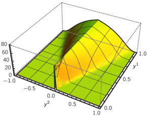
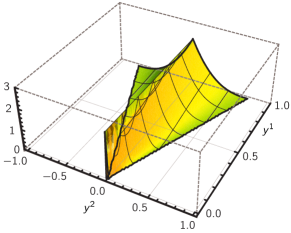
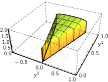
Finally, the dimensionless quantity is plotted in Fig. 2. Some of its properties such as the discontinuity for are directly visible.
V Finsler structures and manifolds
After understanding the properties of the Lagrangian it shall be promoted to a Finsler structure. In general, a Lagrangian depends on velocity components , where for are the spatial components. The underlying metric of the Lagrangian is called and it is used to lower and raise indices, e.g, . It is a pseudo-Riemannian metric with signature , whereas a Finsler structure in dimensions is characterized by a Riemannian metric with signature . First, the defining properties of a Finsler structure shall be reviewed.
Consider an -dimensional manifold with its tangent bundle where , for . The underlying Riemannian metric will be denoted as . is promoted to a Finsler manifold by introducing a function : with where the following properties hold:
-
1)
for (positivity),
-
2)
for (differentiability),
-
3)
for all (positive homogeneity of first degree for ),
-
4)
and the Hessian matrix
(5.1) is positive definite for (strong convexity).
Some texts, e.g., Antonelli:1993 include the first property, whereas it is omitted in Bao:2000 . The function is called the fundamental function, metric function, Lagrangian Antonelli:1993 or simply a Finsler structure Bao:2000 and is named the derived metric, fundamental Finsler tensor or just metric Finsler tensor Antonelli:1993 .
Finsler structures that fulfill the properties of (1) – (4) for all except of at slits (such as the zero section ) are called -global Bao:2000 . If this is not the case they are sometimes denoted as -local; examples for the latter are the -th root Finsler spaces Matsumoto:1996 . Furthermore for the “classical” definition of a Finsler structure the property (4) is crucial. However Matsumoto Matsumoto:1986 and the majority of later authors agree that fundamental tensors, which are invertible but not positive definite, are reasonable extensions of the realm of Finsler geometry Beem:1970 ; Asanov:1985 . In this context the strong convexity condition (4) is replaced by the requirement that and could then be called an indefinite Finsler structure. By doing so, the other conditions can be relaxed as well. It is then sufficient to require with the properties stated above to be defined on a subset of only where the associated are called the “admissible vectors” by some authors Asanov:1985 . Examples for indefinite Finsler metrics will be encountered in what follows.
V.1 Construction of a Finsler structure
According to Kostelecky:2011qz a Finsler structure can be constructed from a Lagrangian by either restricting to the spatial domain or by performing a Wick rotation. The fermion mass is then often set to 1 in this procedure. However it will be kept in what follows such that the mass dimensions of the various terms will not be spoilt. Pursuing the first possibility, the expansions
| (5.2a) | ||||
| (5.2b) | ||||
for lead us to
| (5.3) |
with . The result corresponds to the Finsler structure of Euclidean three-dimensional space (in Cartesian coordinates) being scaled with a dimensionless factor . It is only defined for nonzero although according to the first item in the previous section the Lagrangian corresponds to the standard result for . However note that this limit only exists for time- and lightlike , , where the latter condition is not valid for and considered in Eq. (5.3).
The pole of Eq. (5.3) in can be explained as follows. Considering it is evident that the Lorentz-violating coefficient is directly coupled to the zeroth component of the four-momentum. This translates from the wave packet to the velocity of the classical point particle, which forbids the combined limit and .
The Finsler structure of Eq. (5.3) describes a Euclidean geometry where distances between two points are scaled by the factor in comparison to conventional Euclidean geometry being characterized by the structure . Angles are not affected by the scaling. Note that such a geometry is described by the spatial part of the Friedmann-Lemaître-Robertson-Walker metric (with zero curvature), which has a wide application in cosmological models. In the latter metric there appears a time-dependent scale factor.
The second possibility, i.e., a Wick rotation of the Lagrangian with fails to produce a Finsler structure. It can be demonstrated numerically that does not have a positive definite metric according to Eq. (5.1).111To do so the original expressions obtained from the computer algebra system have to be used instead of Eq. (IV), since the Lagrangian in its latter form is only valid for real , , and . Alternatively an anti-Wick rotation was investigated where and . This did not lead to a positive definite metric either. The reason why this is the case will be explained as follows. The sets and defined in Eqs. (4.10a), (4.10b) separate into two parts with completely different properties. For the limit of a vanishing Lorentz-violating coefficient these sets are given by
| (5.4a) | |||
| (5.4b) | |||
According to Eq. (4.6a) the Lagrangian corresponds to the standard result in the limit of zero if . Hence the Lagrangian describes the physics of a classical, relativistic point particle in the presence of nonminimal Lorentz violation caused by the coefficient only if . Performing a Wick rotation of would lead to and then . However for lying in the latter domain the Lagrangian is not supposed to describe the physics of the same classical point particle. What is then the meaning of in that regime? The answer to this question will be examined as follows.
First of all, for simplicity the further analysis will be restricted to as a function of due to the isotropy of the Lagrangian. Then we define
| (5.5a) | ||||
| (5.5b) | ||||
| (5.5c) | ||||
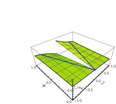
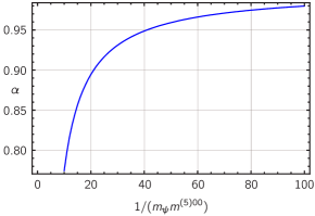
Here the index “(2)” of indicates that this is a two-dimensional function of where , are considered as parameters. The sets , are the two-dimensional restrictions of , of Eqs. (4.10b), (4.10d) to . Note that is the set for which the Lagrangian does not describe the physics of a classical point particle moving in a Lorentz-violating background. It can be determined by computing the zeros of . Due to the homogeneity of the function , to obtain the zeros the ansätze are made where is calculated numerically (see Fig. 3 for a certain range of the Lorentz-violating coefficient).
As a next step the metric corresponding to shall be investigated. It is computed according to Eq. (5.1):
| (5.6) |
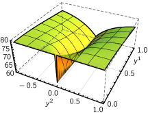
This is an extremely complicated -matrix, which will not be stated explicitly. The computation is straightforward to be done with a computer algebra system, as only derivatives have to be performed. Now the definiteness of this metric shall be checked by calculating its eigenvalues and looking at their signs. Choosing special values for and the Lorentz-violating coefficient , the eigenvalues are plotted in Fig. 4. One can see that the first eigenvalue is larger than zero for the shown range of where the second eigenvalue is most probably positive for .222 Numerically (see also Fig. 3) it follows that are the zeros of the function of Eq. (4.10c) for , which are most probably the lines separating the positive from the negative eigenvalues in Fig. 4b. Hence there exist strong indications that the metric is positive definite for .
Furthermore for and the Lagrangian is for (cf. Eq. (4.13)). In addition, it is positively homogeneous of first degree according to Eq. (6)). Therefore the performed numerical investigations indicate that the Lagrangian itself is a two-dimensional Finsler structure without any Wick rotation at all as long as lies in the domain . Therefore since fulfills the requirements of a Finsler structure on an exceptional set only, it must be considered as a -local Finsler structure. If an indefinite Finsler metric is permitted instead of a positive definite one the latter Lagrangian can be considered as a Finsler structure on a larger set of admissible vectors (cf. the end of Sec. V). However this possibility shall not be studied further.
Now this Finsler structure shall be classified. A first step is to compute the Cartan torsion , which is given by Bao:2004
| (5.7) |
Note that some authors define with an additional prefactor (see, e.g., Bao:2000 ). The mean Cartan torsion is defined as
| (5.8) |
with the inverse Finsler metric . According to a theorem by Deicke a Finsler space is a Riemann space if and only if vanishes Deicke:1953 . Both and can be obtained for Eq. (5.5a). The computation is again straightforward but the result is very lengthy, which is why it will not be given. However it can be demonstrated that does not vanish for certain numerical parameters. For example, with , , and one obtains
| (5.9) |
Hence the Finsler space, which is defined by the Lagrangian for a certain subset of velocities, is definitely not Riemannian.
A further important quantity, which helps to classify Finsler spaces, is the Matsumoto torsion:
| (5.10) |
where is the dimension of the Finsler space to be considered Bao:2004 . The Matsumoto-Hōjō theorem tells us that a Finsler space with dimension is a Randers space, , or a Kropina space, , if and only if the Matsumoto torsion vanishes Matsumoto:1978 . Here and where is a Riemannian metric and a vector field.333 Randers and Kropina spaces are special examples for -spaces. The latter have a fundamental function of the form where is a positive function on an interval such that for all and Bao:2004 . However note that for a two-dimensional Finsler space (see, e.g., exercise (11.2.4) in Bao:2000 ), which is why the Matsumoto-Hōjō theorem cannot be applied. This concludes the analysis of the two-dimensional Finsler structure of Eq. (5.5a).
Finally the following four-dimensional function is considered where :
| (5.11) |
Then analogously to Eq. (5.6) a metric tensor can be constructed again, which is now a -matrix. Its eigenvalues behave similarly to the eigenvalues of the two-dimensional Finsler metric . There are strong numerical indications that all four eigenvalues are positive as long as and therefore the metric is probably positive definite for lying in this domain. Besides, , for , and is positively homogeneous of first degree. This is what makes a Finsler structure for . For this case the mean Cartan torsion, Eq. (5.8), and the Matsumoto torsion of Eq. (5.10) are computed numerically as well. The Cartan torsion does not vanish and at least some of the Matsumoto torsion coefficients are not equal to zero. Numerical results for the mean Cartan torsion and the nonvanishing Matsumoto torsion coefficients for , , , and are given by:
| (5.12a) | ||||
| (5.12b) | ||||
| (5.12c) | ||||
| (5.12d) | ||||
| (5.12e) | ||||
| (5.12f) | ||||
| (5.12g) | ||||
This shows that Eq. (5.11) is neither a Riemann nor a Randers/Kropina structure, since now the Matsumoto-Hōjō theorem can be applied. Therefore it is a further, though complicated, example for a Finsler space with these properties in the context of the SME. An alternative example is the b-structure
| (5.13) |
where are the CPT-odd, pseudovector fermion coefficients of the minimal SME. The latter is given in Eqs. (5), (6) of Kostelecky:2011qz by setting the CPT-odd vector coefficients equal to zero. Besides, further structures with nonvanishing Matsumoto torsion have been found such as the bipartite structures given by Eq. (9) in Kostelecky:2012ac and a structure that is formed from a particular choice of the minimal, CPT-odd tensor coefficients , cf. Eq. (35) in Colladay:2012rv .
Finally along the derivation of the Lagrangian in App. A the remaining two complex roots can be taken into account in . The Lagrangian that results from taking the second/third root of unity in will be denoted as and , respectively. From these Lagrangians the derived metrics will be computed based on Eq. (5.1):
| (5.14a) | ||||
| (5.14b) | ||||
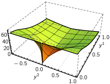
where the replacements and have been performed. Figures 5a and 5b show numerical results for the eigenvalues of where . The first eigenvalue of is presented in Fig. 5c where the second eigenvalue is largely negative such as the first one and therefore has been omitted. The results suggest that both eigenvalues of are positive. Besides it can be checked that for , whereas for all and . This turns into a -local Finsler structure as well. It seems that corresponds to the standard Lagrangian (modulo a global sign) for , which complements the result of Eq. (4.6a).
VI Physical Implications
The dynamics of a classical particle corresponding to the dispersion relation of Eq. (2.2) can in principle be found by interpreting the left-hand side of the dispersion law as the Hamiltonian of the particle. Integrating the Hamilton equations will then result in the particle trajectories. However since the connection to Finsler geometry shall be outlined in this article, the positively homogeneous Lagrangian in Eq. (IV) will be taken as a basis to discuss the physics. Its complexity makes it difficult to study its physical properties for an arbitrarily large Lorentz-violating coefficient . Therefore using the relations of Eq. (B.1), the Lagrangian will be expanded in the dimensionless quantity when assuming the latter to be much smaller than one. This gives the following more transparent result:
| (6.15) |
Hence at first order in the Lorentz-violating coefficient the Lagrangian is characterized by an additional isotropic contribution, which involves the observer Lorentz scalar . Furthermore it is proportional to the square of the zeroth four-velocity component, which is reasonable, since in momentum space couples to . The result can be compared to the Lagrangian of Eq. (28) in Girelli:2006fw , which was obtained for the modified dispersion relation of their Eq. (22). The latter involves an additional term cubic in the particle momentum. The Lorentz-violating contribution of their Lagrangian is a function of as well. However it is proportional to the cube of the velocity, which mirrors the modified momentum dependence of their dispersion relation.
The intention now is to understand the physics of Eq. (VI). Therefore we consider a classical particle with mass moving along a trajectory parameterized such that and where is the speed of light and the conventional three-velocity. Note that is set equal to one. The classical Lagrangian can then be written in the form
| (6.16) |
with higher-order terms in the Lorentz-violating coefficient neglected. If the particle is free it still moves on a straight line such as in the conventional case. Therefore it will be assigned an electric charge and it will be coupled to a four-potential . Then the Lagrangian describing the propagation of this charged, classical particle (with its position ) in an electromagnetic field is given by
| (6.17) |
with of Eq. (6.16). The Euler-Lagrange equations read as follows:
| (6.18a) | ||||
| (6.18b) | ||||
with the Lorentz factor . Here the electric and magnetic fields , have been introduced according to
| (6.19) |
Now different physical situations can be considered, e.g., the particle moving in a constant magnetic field and a vanishing electric field, , with the initial conditions and . Here is the magnitude of the velocity and is the distance of the particle from the origin at the beginning. Since a magnetic field does not change the energy or the Lorentz factor of the particle, the equations of motion in this case read as follows:
| (6.20) |
By plugging in the Ansatz
| (6.21) |
one can demonstrate that the particle still moves on a circle of radius such as in the conventional case where the cyclotron frequency is modified as follows:
| (6.22) |
Physically this can be interpreted as the particle having a slightly different mass . The modification of the mass is velocity-dependent via the gamma-factor, i.e., for an increasing velocity the Lorentz-violating effects get enhanced. Note that a constant rescaling of the particle mass could not be observed. However since this rescaling has an additional velocity dependence, this would modify the velocity dependence of the cyclotron frequency leading to an experimentally observable effect.
The situation is similar for a particle moving along a constant electric field (where ) with the initial conditions , . In the relativistic case the corresponding differential equation can be solved, but the result is rather involved and not very illuminating. Therefore the nonrelativistic case will be considered with leading to the result
| (6.23) |
Here the velocity-dependent mass of Eq. (6.22) appears as well (with ). The interpretation of these results is as follows. In the modified dispersion law of Eq. (2.2), which the current paper is based on, two additional factors of the particle energy are associated to the nonminimal Lorentz-violating coefficient leading to a quartic polynomial in . This holds in phase space, i.e., the cotangent space of the underlying manifold. The connection to the tangent space is that is linked to two additional factors of . The latter corresponds to the standard relativistic energy of the particle being expressed by the particle velocity. Note that for a sufficiently large velocity the mass would become negative. The reason is that the Lagrangian considered is a good approximation only for a sufficiently small Lorentz-violating coefficient. The Lorentz-violating effects become stronger for increasing velocity and we then move outside of the domain where the expansion is valid.
The next step is to understand the conserved quantities according to the lines of Girelli:2006fw . Using Eq. (3.2) the conjugate momentum can be obtained from the Lagrangian and it reads as follows:
| (6.24) |
Here the preferred timelike direction was introduced to write the result in a covariant way. Furthermore via Eq. (5.1) a pseudo-Finsler metric can be constructed with the fundamental function chosen to be the Lagrangian:
| (6.25) |
Using the Finsler metric, the conserved quantities are obtained via Eq. (35) in Girelli:2006fw . Apart from an additional factor of where the minus sign comes from the definition of the canonical momentum used in the current paper (see Eq. (36) in Girelli:2006fw ) these conserved quantities correspond to the energy and three-momentum directly obtained from Eq. (6.24):
| (6.26a) | ||||
| (6.26b) | ||||
Note that for sufficiently high velocities the energy can become negative, too. Looking at the left-hand side of Eq. (6.18b) it can be seen that Eq. (6.26b) is, indeed, the particle momentum. If there are no external forces both the energy and the momentum is conserved, as expected, which is why the particle then moves on a straight line. This demonstrates some of the results of Girelli:2006fw for the particular Lagrangian of Eq. (6.16).
A treatment of the exact Lagrangian of Eq. (IV) along the lines above is out of reach with such analytical tools. In principle higher-order effects in the Lorentz-violating coefficient could be studied by taking into account additional coefficients in the series expansion of Eq. (VI). Including two more coefficients results in the Lagrangian
| (6.27) |
Hence this leads to higher-order terms in the Lorentz factor (and particle velocity) coupled to the Lorentz-violating coefficient, which changes the behavior for velocities approaching the speed of light. That probably also cures the properties of the new particle mass and the energy such that they do not become negative for an increasing velocity. For growing momenta the Lorentz-violating effects in the modified dispersion relation of Eq. (2.2) are enhanced, i.e., the behavior observed is again the corresponding analogue in the tangent space. Furthermore in Girelli:2006fw it was stated that the Finsler structure, which is seen by the propagating particle, depends on the particle mass. Such effects are observed here as well. For example, the modification of the particle mass, cf. Eq. (6.22), would be larger for a muon compared to an electron.
VII Conclusions and outlook
To summarize, in this paper the Lagrangian was obtained for a classical, relativistic point particle whose conjugate momentum fulfills the modified dispersion relation of a quantum wave packet underlying Lorentz violation caused by an isotropic dimension-5 operator. The speciality is that it was possible to obtain the momentum-velocity correspondence and, therefore, the Lagrangian directly without having to solve a polynomial equation of high degree. This behavior is different from all cases of the minimal SME fermion sector that have been investigated in the literature so far. It is traced back to the isotropic nature of the coefficient considered and it is expected to be possible in general as long as an isotropic Lorentz-violating framework is taken as a basis of the studies carried out.
Having obtained the Lagrangian its properties were discussed. The Lagrangian can be positive, zero or negative in certain domains of the four-velocity components plus it is apart from the region that has to be excluded. It corresponds to the standard Lagrangian for a vanishing Lorentz-violating coefficient as long as the four-velocity is time- or lightlike. For this reason it describes the physics of a classical, relativistic point particle only for a certain domain of four-velocities.
The final goal was to promote the Lagrangian to a Finsler structure and to understand its characteristics. Restricting the Lagrangian to the spatial domain results in a Finsler structure describing a scaled Euclidean geometry. Performing a Wick rotation fails to produce a Finsler structure. However, interestingly the Lagrangian itself is a Finsler structure for four-velocity components lying in a subset of the domain where it does not describe the physics of a point particle. It was demonstrated that this Finsler structure is neither a Riemann nor a Randers or Kropina structure.
Finally the Lagrangian was expanded to first order in the Lorentz-violating coefficient and its physical properties were discussed. To carry this out, both the Finsler metric and the canonical momentum were calculated, which were used to obtain the conserved quantities for free motion of the particle. Furthermore the particle was assigned an electric charge and its propagation in constant electric and magnetic fields was analyzed. Due to the Lorentz-violating background the particle acquires a modified mass, which additionally depends on the velocity.
One last comment shall note a possible connection to Meister:1989vf . In the latter reference it is shown that certain complex Riemannian manifolds have real slices of all possible signatures. The Lagrangian considered might provide such an example for Finsler spaces, if it can be embedded into a complex Finsler manifold. Then both the Lagrangian of Eq. (IV) restricted to the domain and the Finsler structure of Eq. (5.11) restricted to the domain may be real slices of the complex Finsler manifold with different signatures. This is an interesting open problem for future studies.
The current paper forms one part of the investigations carried out so far whose purpose is to link the SME to Finsler spaces. These spaces are the most natural framework when studying the motion of a particle in a Lorentz-violating background field. For example, this concerns the physical problem of a charged particle (with spin) moving in a superposition of an electromagnetic field and a Lorentz-violating background field, which is still to be solved. With the knowledge on the correspondence of certain SME sectors to particular Finsler spaces, this and similar physical problems can be tackled smartly that may otherwise be difficult or impractical to solve.
In fact, the application to physical situations is the main goal of the research carried out. But to achieve this, there has to be a mathematical basis and there are still quite some mathematical and theoretical questions whose answers are unknown. For this purpose it is important to perform such analyses, the current one included. Therefore the future plan is to obtain and study the classical Lagrangians and Finsler structures for alternative sets of nonminimal Lorentz-violating coefficients. A special interest lies in Lagrangians having a simpler form compared to the one considered in this paper.
VIII Acknowledgments
It is a pleasure to thank V. A. Kostelecký for reading the manuscript and giving helpful suggestions. Furthermore the author is indebted to N. Russell for helpful discussions. Special thanks is due to the referees for useful comments on the contents and the suggestion of additional references. This work was performed with financial support from the Deutsche Akademie der Naturforscher Leopoldina within Grant No. LPDS 2012-17.
Appendix A Obtaining the classical Lagrangian
Finding the zeros of the third-order polynomial mentioned below Eq. (4.1) in Sec. IV results in the following complicated expression for the particle energy as a function of the four-velocity components:
| (A.1a) | ||||
| (A.1b) | ||||
| (A.1c) | ||||
| (A.1d) | ||||
| (A.1e) | ||||
| (A.1f) | ||||
The cubic roots in this expression make it quite involved to check whether is a real quantity. However can be written in a surprisingly compact form as follows, which is more suitable to evaluate these roots:
| (A.2a) | ||||
| (A.2b) | ||||
| (A.2c) | ||||
From Eq. (A.1a) we see that in this expression there appears the third root of the complex quantity . The third roots of unity of will be denoted as for . We then obtain
| (A.3a) | ||||
| (A.3b) | ||||
Now a part of the expression under the square root in Eq. (A.1a) collapses to a convenient result:
| (A.4) |
Finally taking the first of the third roots of unity labeled with , Eq. (A.1a) can be brought into the form that has been stated in Eq. (4.2a):
| (A.5) |
Putting together the previous and of Eq. (4.2a) and introducing the function of Eq. (4.3a) for brevity leads to the Lagrangian of Eq. (IV):
| (A.6) |
Appendix B Properties of the classical Lagrangian
B.1 Limit for vanishing Lorentz-violating coefficient
To obtain the limit of the Lagrangian, Eq. (IV), we consider the following identities whose validity has been checked numerically:
| (B.1a) | ||||
| (B.1b) | ||||
where the second equation only holds for . The radicand under the square root of Eq. (IV) can then be expanded with respect to . Using the identities above one can show that the first and second term in this expansion vanish and that the leading contribution is of order :
| (B.2) |
The leading contribution in the term behind the square root is independent of :
| (B.3) |
The result for a vanishing Lorentz-violating coefficient is then
| (B.4) |
which is the result of Eq. (4.6a) with the sign function given by Eq. (4.6b)
B.2 Differentiability of the Lagrangian
We consider the argument of the inverse cosine in Eq. (IV) and we want to show that the image of is the interval . Partial differentiation with respect to and , respectively, gives:
| (B.5a) | ||||
| (B.5b) | ||||
Both derivatives vanish for , , and . The Hessian matrices evaluated at the sets mentioned show that these are extrema with the values
| (B.6a) | ||||
| (B.6b) | ||||
So at , there are minima, whereas at there are maxima. The latter take their maximum value 1 for and for perturbative Lorentz violation they are larger than zero. This shows that takes values within where is differentiable for its argument lying in (-1,1). So the lines { and have to be removed to keep the Lagrangian differentiable.
References
- (1) P. Finsler, Über Kurven und Flächen in allgemeinen Räumen, in German (Gebr. Leemann & Co., Zürich, 1918).
- (2) É. Cartan, Sur les espaces de Finsler, in French, C. R. Acad. Sci. (Paris) 196, 582 (1933).
- (3) É. Cartan, Les espaces de Finsler (Herman et Cie, Paris, 1934).
- (4) S.-S. Chern, “Finsler geometry is just Riemannian geometry without the quadratic restriction,” Notices of the AMS 43, 959 (1996).
- (5) P. L. Antonelli, R. S. Ingarden, and M. Matsumoto, The Theory of Sprays and Finsler Spaces with Applications in Physics and Biology (Springer Science + Business Media, Dordrecht, 1993).
- (6) D. Bao, S.-S. Chern, and Z. Shen, An Introduction to Riemann-Finsler Geometry (Springer, New York, 2000).
- (7) H. Busemann, “The geometry of Finsler spaces,” Bull. Amer. Math. Soc. 56, 5 (1950).
- (8) L. Kozma and L. Tamássy, “Finsler geometry without line elements faced to applications,” Rep. Math. Phys. 51, 233 (2003).
- (9) V. A. Kostelecký and S. Samuel, “Spontaneous breaking of Lorentz symmetry in string theory,” Phys. Rev. D 39, 683 (1989).
- (10) V. A. Kostelecký and R. Potting, “CPT and strings,” Nucl. Phys. B 359, 545 (1991).
- (11) V. A. Kostelecký and R. Potting, “CPT, strings, and meson factories,” Phys. Rev. D 51, 3923 (1995), hep-ph/9501341.
- (12) V. A. Kostelecký and R. Potting, “Expectation values, Lorentz invariance, and CPT in the open bosonic string,” Phys. Lett. B 381, 89 (1996), hep-th/9605088.
- (13) D. Colladay and V. A. Kostelecký, “Lorentz violating extension of the standard model,” Phys. Rev. D 58, 116002 (1998), hep-ph/9809521.
- (14) V. A. Kostelecký and M. Mewes, “Electrodynamics with Lorentz-violating operators of arbitrary dimension,” Phys. Rev. D 80, 015020 (2009), arXiv:0905.0031 [hep-ph].
- (15) V. A. Kostelecký and M. Mewes, “Neutrinos with Lorentz-violating operators of arbitrary dimension,” Phys. Rev. D 85, 096005 (2012), arXiv:1112.6395 [hep-ph].
- (16) V. A. Kostelecký and M. Mewes, “Fermions with Lorentz-violating operators of arbitrary dimension,” Phys. Rev. D 88, 096006 (2013), arXiv:1308.4973 [hep-ph].
- (17) V. A. Kostelecký and N. Russell, “Classical kinematics for Lorentz violation,” Phys. Lett. B 693, 443 (2010) arXiv:1008.5062 [hep-ph].
- (18) D. Colladay and P. McDonald, “Classical Lagrangians for momentum dependent Lorentz violation,” Phys. Rev. D 85, 044042 (2012), arXiv:1201.3931 [hep-ph].
- (19) N. Russell, “Finsler-like structures from Lorentz-breaking classical particles,” Phys. Rev. D 91, 045008 (2015), arXiv:1501.02490 [hep-th].
- (20) V. A. Kostelecký, “Riemann-Finsler geometry and Lorentz-violating kinematics,” Phys. Lett. B 701, 137 (2011), arXiv:1104.5488 [hep-th].
- (21) V. A. Kostelecký, N. Russell, and R. Tso, “Bipartite Riemann-Finsler geometry and Lorentz violation,” Phys. Lett. B 716, 470 (2012), arXiv:1209.0750 [hep-th].
- (22) G. Randers, “On an asymmetrical metric in the four-space of general relativity,” Phys. Rev. 59, 195 (1941).
- (23) E. Caponio, M. A. Javaloyes, and A. Masiello, “On the energy functional on Finsler manifolds and applications to stationary spacetimes,” Math. Ann. 351, 365 (2011), math/0702323 [math.DG].
- (24) E. Caponio, M. A. Javaloyes, and M. Sánchez, “On the interplay between Lorentzian causality and Finsler metrics of Randers type,” Rev. Mat. Iberoam. 27, 919 (2011), arXiv:0903.3501 [math.DG].
- (25) B. Russell and S. Stepney, “Zermelo navigation and a speed limit to quantum information processing,” Phys. Rev. A 90, 012303 (2014), arXiv:1310.6731 [quant-ph].
- (26) G. W. Gibbons, C. A. R. Herdeiro, C. M. Warnick, and M. C. Werner, “Stationary metrics and optical Zermelo-Randers-Finsler geometry,” Phys. Rev. D 79, 044022 (2009), arXiv:0811.2877 [gr-qc].
- (27) E. Caponio, A. V. Germinario, and M. Sánchez, “Convex regions of stationary spacetimes and Randers spaces. Applications to lensing and asymptotic flatness,” J. Geom. Anal. (2015), arXiv:1112.3892 [math.DG].
- (28) M. C. Werner, “Gravitational lensing in the Kerr-Randers optical geometry,” Gen. Rel. Grav. 44, 3047 (2012), arXiv:1205.3876 [gr-qc].
- (29) J. Skákala and M. Visser, “Pseudo-Finslerian spacetimes and multi-refringence,” Int. J. Mod. Phys. D 19, 1119 (2010), arXiv:0806.0950 [gr-qc].
- (30) T. Kawaguchi, “On the application of Finsler geometry to engineering dynamical systems,” Per. Math. Hung. 8, 281 (1977).
- (31) I. Bucataru and R. Mirson, Finsler-Lagrange geometry. Applications to dynamical systems (Ed. Acad., Bucharest, 2007).
- (32) L. Astola and L. Florack, “Finsler geometry on higher order tensor fields and applications to high angular resolution diffusion imaging,” Int. K. Comput. Vis. 92, 325 (2011).
- (33) C. Pfeifer and M. N. R. Wohlfarth, “Causal structure and electrodynamics on Finsler spacetimes,” Phys. Rev. D 84, 044039 (2011), arXiv:1104.1079 [gr-qc].
- (34) C. Pfeifer and M. N. R. Wohlfarth, “Finsler spacetimes and gravity,” Springer Proc. Phys. 157, 305 (2014), arXiv:1210.2973 [gr-qc].
- (35) C. Pfeifer and M. N. R. Wohlfarth, “Finsler geometric extension of Einstein gravity,” Phys. Rev. D 85, 064009 (2012), arXiv:1112.5641 [gr-qc].
- (36) C. Pfeifer and M. N. R. Wohlfarth, “Beyond the speed of light on Finsler spacetimes,” Phys. Lett. B 712, 284 (2012), arXiv:1109.6005 [gr-qc].
- (37) M. Hohmann, “Extensions of Lorentzian spacetime geometry: From Finsler to Cartan and vice versa,” Phys. Rev. D 87, 124034 (2013), arXiv:1304.5430 [gr-qc].
- (38) H. E. Brandt, “Quantum fields in the space-time tangent bundle,” Found. Phys. Lett. 11, 265 (1998).
- (39) H. E. Brandt, “Finslerian quantum fields and microcausality,” Found. Phys. Lett. 13, 307 (2000).
- (40) L. Zhang and X. Xue, “The Finsler type of space-time realization of deformed very special relativity,” arXiv:1205.1134 [math-ph].
- (41) V. Perlick, “Fermat principle in Finsler spacetimes,” Gen. Rel. Grav. 38, 365 (2006), gr-qc/0508029.
- (42) R. G. Torromé, P. Piccione, and H. Vitório, “On Fermat’s principle for causal curves in time oriented Finsler spacetimes,” J. Math. Phys. 53, 123511 (2012), arXiv:1202.3869 [math.DG].
- (43) R. G. Torromé and J. Gratus, “On -jet field approximations of geodesic deviation equations,” arXiv:1301.6352 [math-ph].
- (44) M. A. Javaloyes and M. Sánchez, “Finsler metrics and relativistic spacetimes,” Int. J. Geom. Meth. Mod. Phys. 11, 1460032 (2014), arXiv:1311.4770 [math.DG].
- (45) M. Schreck, “Quantum field theoretic properties of Lorentz-violating operators of nonrenormalizable dimension in the fermion sector,” Phys. Rev. D 90, 085025 (2014), arXiv:1403.6766 [hep-th].
- (46) D. Colladay and V. A. Kostelecký, “Cross sections and Lorentz violation,” Phys. Lett. B 511, 209 (2001), hep-ph/0104300.
- (47) M. Matsumoto, “Theory of Finsler spaces with -th root metric II,” Publ. Math. Debrecen 49, 135 (1996).
- (48) M. Matsumoto, Foundations of Finsler geometry and special Finsler spaces (Kaiseisha Press, Japan 1986).
- (49) J. K. Beem, “Indefinite Finsler spaces and timelike spaces,” Cna. J. Math. 22, 1035 (1970).
- (50) G. S. Asanov, Finsler Geometry, Relativity and Gauge Theories (D. Reidel Publishing Company, Dordrecht, 1985).
- (51) Z. Shen, “Landsberg curvature, -curvature and Riemann curvature,” in A Sampler of Riemann-Finsler Geometry, edited by D. Bao, R. L. Bryant, S.-S. Chern, and Z. Shen, Math. Sci. Res. Inst. Publ. 50 (Cambridge University Press, Cambridge New York Port Melbourne Madrid Cape Town, 2004).
- (52) A. Deicke, “Über die Finsler-Räume mit ,” in German, Arch. Math. 4, 45 (1953).
- (53) M. Matsumoto and S. Hōjō, “A conclusive theorem on C-reducible Finsler spaces,” Tensor (N.S.) 32, 225 (1978).
- (54) F. Girelli, S. Liberati, and L. Sindoni, “Planck-scale modified dispersion relations and Finsler geometry,” Phys. Rev. D 75, 064015 (2007), gr-qc/0611024.
- (55) A. Meister, “Complex manifold methods in quantum field theory in curved space-time,” J. Math. Phys. 30, 2930 (1989).