Numerical Study of a Many-Body Localized System Coupled to a Bath
Abstract
We use exact diagonalization to study the breakdown of many-body localization in a strongly disordered and interacting system coupled to a thermalizing environment. We show that the many-body level statistics cross over from Poisson to GOE, and the localized eigenstates thermalize, with the crossover coupling decreasing with the size of the bath in a manner consistent with the hypothesis that an infinitesimally small coupling to a thermodynamic bath should destroy localization of the eigenstates. However, signatures of incomplete localization survive in spectral functions of local operators even when the coupling to the environment is sufficient to thermalize the eigenstates. These include a discrete spectrum and a gap at zero frequency. Both features are washed out by line broadening as one increases the coupling to the bath. We also determine how the line broadening scales with coupling to the bath.
pacs:
78.40.Pg, 71.23.An, 71.30.+h, 72.80.NgIsolated quantum systems with quenched disorder can enter a ‘localized’ regime where they fail to ever reach thermodynamic equilibrium anderson . While we have an essentially complete understanding of localization in non-interacting systems anderson , the theory of many-body localization (MBL) is still under construction AKGL (1997); Mirlin (2006); BAA (2006); Oganesyan (2008); Prosen (2008); Pal (2010); Imbrie (2014); LPQO (2013); Bauer (2013); Pekker (2013); Vosk (2013); narrowbath (2014); Bahri (2013); Lbits (2013); serbyn ; Abanin (2013); QHMBL (2014); Sid (2014); Bauer2 (2014); arcmp ; altmanreview (2014). Numerical investigations using exact diagonalization Oganesyan (2008); Pal (2010); serbyn do indicate that all eigenstates of a strongly interacting disordered system can be localized. Most of the theoretical research so far has been in the limit of a perfectly isolated system. However, experimental tests of MBL (shahar ; demarco ) will always include some finite coupling to the environment. What then can we expect to see in experiments designed to probe many body localization?
A recent theory of MBL systems weakly coupled to heat baths proposed that while eigenstates are delocalized by an infinitesimally weak coupling to a heat bath, signatures of localization persist in spectral functions of local operators for weak coupling to a bath rahul . This theory has yet to face stringent numerical tests. Moreover, it did not discuss the spectral functions of the physical degrees of freedom, the quantities of direct relevance for experiments, focusing instead on the spectral functions of certain localized integrals of motion that are believed to exist serbyn ; Imbrie (2014); Lbits (2013), but which are related to the physical degrees of freedom by an unknown unitary transformation. This work directly addresses these issues.
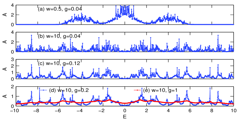
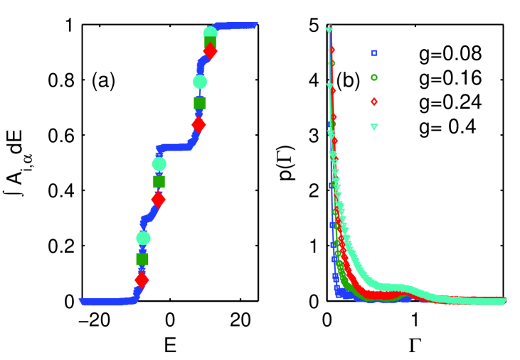
We use exact numerical diagonalization to establish the behavior of many body localized systems weakly coupled to heat baths. We show that coupling to a bath results in a crossover from Poisson to Gaussian orthogonal ensemble (GOE) eigenvalue statistics, which becomes exponentially steeper with increasing bath size. A similar rapid crossover to thermalization is seen in the eigenstates. However, the prospect for seeing MBL in experiments is still realistic because signatures of incomplete localization remain in the spectral functions of local (in real space) operators. Indeed, we find that the spectral functions of the microscopic degrees of freedom look completely different in the localized and thermal phases (see Fig. 1). The thermal phase has a continuous spectrum whereas the local spectral function in the localized phase is discrete, with a hierarchy of gaps, and a gap at zero frequency that survives even after spatial averaging. Increasing causes lines to broaden and fill in these gaps. However, as long as the typical line broadening is less than the largest gaps, gap-like features remain. Our work also reveals how the line broadening scales with .
The model: We choose the antiferromagnetic Heisenberg spin- chain with random fields along :
| (1) |
We set the interaction . The on-site fields are independent random variables, uniformly distributed between and ; measures the disorder strength in the system. This model with periodic boundary conditions has been shown to have a many-body localization transition at in the infinite temperature limit Pal (2010).
The Hamiltonian in Eq. 1 is written in terms of the physical degrees of freedom (‘-bits,’ in the language of Lbits (2013), where =physical). In general, its eigenstates are quite complicated and non-trivial. As shown Lbits (2013); serbyn , one can perform a unitary transformation to rewrite in terms of localized constants of motion . The are dressed versions of the operators, which are localized in real space, with exponential tails, and are referred to in Lbits (2013) as ‘-bits’ (=localized). A unitary transformation to this ‘-bit’ basis can always be performed, if the system is in the regime where all the many body eigenstates are localized. In this -bit basis, the Hamiltonian becomes
| (2) |
The values of the coefficients and will depend upon the parent Hamiltonian (1), although these coefficients all fall off exponentially with distance. The eigenstates of (2) are just products of .
Motivated by the representation (2) of the Hamiltonian (1), it is instructive to consider the simpler Hamiltonian
| (3) |
where the and as independent random variables taken from a log-normal distribution with and , and similarly for . We take and work with open-boundary conditions. This Hamiltonian also has the feature that eigenstates are product states of , and is simpler to work with numerically.
For the bath, we use a non-integrable Hamiltonian that has been recently studied kim . It consists of interacting spins with the Hamiltonian:
| (4) |
While using open boundary conditions, we add a boundary term to . We use , and , values for which has been numerically shown by kim to have fast entanglement spreading. (We use periodic boundary conditions only for -bits with .)
The interaction between the system and bath should be local for both - and -bits. We first study -bit eigenstates, choosing the coupling:
| (5) |
Later we examine -bit spectra, using the coupling
| (6) |
The total Hamiltonian is thus , where and are given by Eq. (3) and (5) in the first part of this work, and by Eq. (1) and (6) in the latter part of this work. We will indicate the transition clearly in the text. We use open boundary conditions except where periodic boundaries are explicitly mentioned.
We start by analyzing the breakdown of localization when the -bit Hamiltonian (3) is coupled to a bath according to (5), by examining the many-body eigenvalue statistics as is increased from . We perform exact diagonalization on a system with spins coupled to spins in the bath. The many body level-spacing is , where is the energy of the th eigenstate. Following Pal (2010), we define the ratio of adjacent gaps as . We average this over eigenstates and several different realizations of the disorder to get a probability distribution at a particular value of . In Fig. 2, we show how evolves from Poisson to GOE like as is increased. In a localized system we expect that , and for a thermalizing system, we expect that .
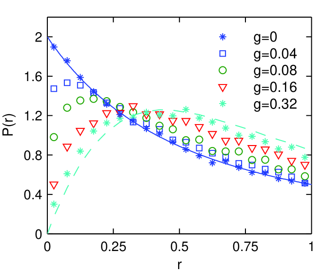
The transition from Poisson to GOE statistics happens gradually for this finite size system. A simple analytical estimate of the characteristic value of at the crossover point proceeds as follows (see also rahul ): If is the bandwidth of the bath and is the many body level spacing in the bath, then the system couples to states, with a typical matrix element to each state of order . The coupling to the bath will be effective in thermalizing the system when this matrix element becomes of order the level spacing in the bath, i.e. when . This indicates that the crossover coupling . Since , the critical value of is expected to scale as .
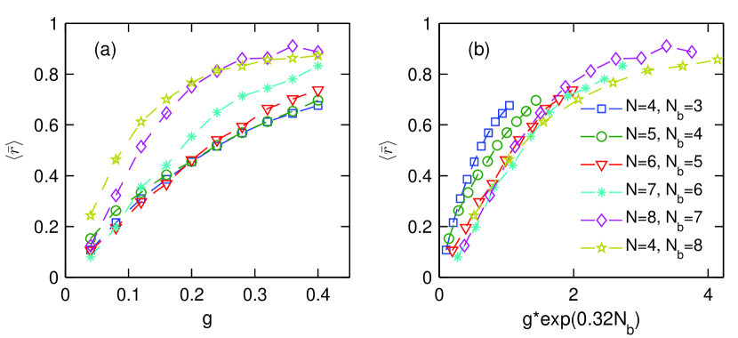
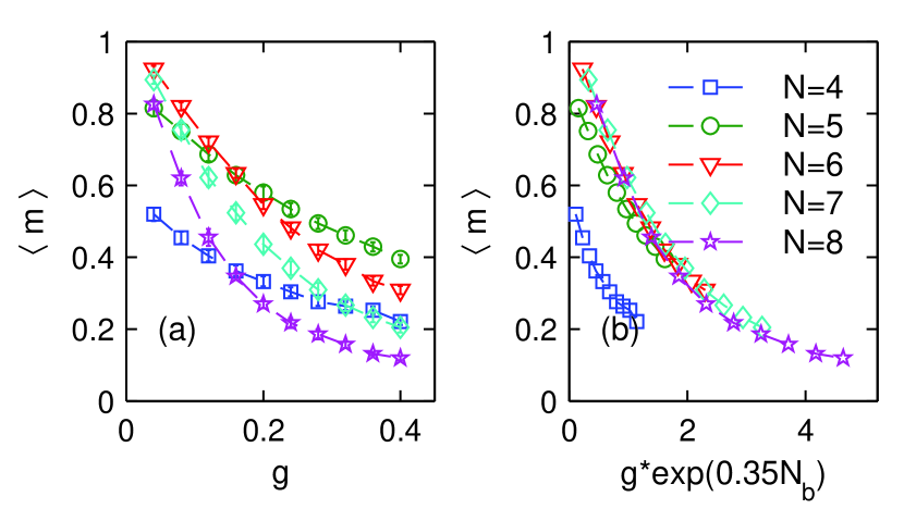
To quantitatively compare this crossover estimate to the data, we define . After averaging over disorder distributions, should be in the GOE regime and in the localized regime Pal (2010). It is convenient to define the normalized quantity =(, such that if the level statistics are GOE and if they are Poisson. Fig. 3(a) shows how varies with for systems of size . Fig. 3(b) shows that scaling of the form is successful in making the data for different in Fig. 3(a) collapse onto one curve. Data collapse occurs also for and , indicating clearly that it is which controls the finite size scaling. We get the best collapse when the constant in the exponential is which is in good agreement with the analytical estimate . This implies that the crossover to thermalization is at a coupling that is exponentially small in system size, so that level statistics become GOE at infinitesimal in the thermodynamic limit.
Another test of thermalization is checking whether the eigenstates obey the eigenstate thermalization hypothesis (ETH) srednicki ; Deutsch (1991); Rigol (2008). The ETH states that the expectation value of a local operator should be the same in every eigenstate within a small energy window. For a localized system this will not be the case. In Fig. 4, we show how eigenstate thermalization sets in as is increased. We choose an energy window around the center of the band and calculate the standard deviation of the expectation value of for all eigenstates within the window. Explicitly, we define
| (7) |
where the overline denotes averaging over an energy window of width in the middle of the band and is an eigenstate of the coupled system and bath. We choose . After averaging over disorder distributions, we expect to find for a thermalized system. Fig. 4(a) shows how approaches 0 as is increased for different system sizes. Fig. 4(b) shows that scales with similar to . The exponent here is , also close to the estimated analytical value.
We now turn to an analysis of the spectral functions of local operators. Henceforth we are working with the physical degrees of freedom, Eq. (1) and (6). We examine the spectral function from an exact eigenstate
| (8) |
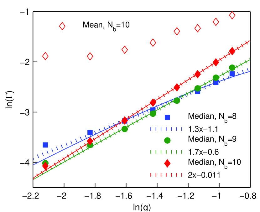
where is the eigenstate of the combined system and bath. We note that since we are working with a finite size system with a discrete spectrum, the spectral function will always consist of a set of delta functions. At , the delta functions should have minimum spacing , equal to the many body level spacing in the system. At non-zero , each ‘parent’ delta function will split into exponentially many descendants, with a typical spacing . A fine binning in energy with bin size greater than will then yield a smooth spectral function, with the ‘parent’ delta functions of the system having been ‘broadened’ by coupling to the bath. To investigate this broadening, it is convenient to take . We therefore take and , and investigate how the ‘line broadening’ evolves with for . Details of the procedure are outlined in the supplementary material, and the results are illustrated in Fig. 5 for . The mean and median linewidth at a particular value of are significantly different. This is a result of the long tails in the distribution of the linewidth (see supplement). Fig. 5 shows that at the larger values of we study, a log-log plot of the median vs appears to fit well to a straight (dashed) line. For the system sizes that we are able to access, the straight line fit suggests , where increases as the size of the bath increases, reaching for . We note that while a simple application of the golden rule predicts , a more careful analysis rahul suggests that the true scaling should be . The solid lines in Fig. 5 are a fit to this theoretical prediction, and are consistent with the data, except at smallest . The discrepancy at smallest and the difference between median and mean are worthwhile topics for future work.
Finally, we analyze the behavior of the spectral function averaged over all sites and eigenstates of the system, for . We note that the Hamiltonian (1) has a delocalization-localization phase transition at . Fig. 1(a) shows on the delocalized side of the transition for a small value of . is smooth everywhere. (The graininess is a result of the small system size.) Fig. 1(b) is on the localized side of the transition, with the system almost decoupled from the bath. Here, consists of clusters of narrow spectral lines, with a hierarchy of energy gaps, just as was shown to be the case for -bit spectral functions in rahul . vanishes at . Thus, local spectral functions can distinguish between extended and localized phases. In Fig. 1(c-e) we examine how the -bit spectral functions evolve as increases. We see that the line broadening increases and different lines start to overlap with each other, washing out the weaker spectral features, but larger gaps remain. The zero-frequency gap also fills in with increasing . The spectral functions retain signatures of localization even for when the eigenstates of the combined system and bath are effectively thermal, and get washed out when becomes comparable to the characteristic energy scales in the system (i.e. ).
In conclusion, we have investigated the signatures of localization in a disordered system weakly coupled to a heat bath using exact diagonalization. The wave functions are found to exhibit a crossover to thermalization as a function of coupling to the bath. The crossover coupling is proportional to the many body level spacing in the bath, and vanishes exponentially fast in the limit of a large bath size. In contrast, the spectral functions of local operators are found to show more robust signatures of proximity to a localized phase. While the spectral functions are smooth and continuous in the delocalized phase (after coarse graining on the scale of the many body level spacing), the spectral functions in the localized phase consist of narrow spectral lines, and contain a hierarchy of gaps, as well as a gap at zero frequency that persists even after spatial averaging. Increasing the coupling to the bath increases the line broadening (in a manner that we calculate) and washes out these features. However, signatures of localization survive in the spectral functions even at couplings to the bath where the exact eigenstates are effectively thermal (Fig. 1).
Acknowledgments: RN would like to thank Sarang Gopalakrishnan and David Huse for a collaboration on related ideas. This work was supported by DOE grant DE-SC0002140. RNB. acknowledges the hospitality of the Institute for Advanced Study, Princeton while this work was being done. RN was supported by a PCTS fellowship. SJ was supported by the Porter Ogden Jacobus Fellowship of Princeton University.
References
- (1) P. W. Anderson, Phys. Rev. 109, 1492 (1958).
- AKGL (1997) B. L. Altshuler, Y. Gefen, A. Kamenev and L. S. Levitov, Phys. Rev. Lett. 78, 2803 (1997).
- Mirlin (2006) I. V. Gornyi, A. D. Mirlin and D. G. Polyakov, Phys. Rev. Lett. 95, 206603 (2005).
- BAA (2006) D. M. Basko, I. L. Aleiner and B. L. Altshuler, Annals of Physics 321, 1126 (2006).
- Oganesyan (2008) V. Oganesyan and D. A. Huse, Phys. Rev. B 75, 155111 (2007).
- Prosen (2008) M. Znidaric, T. Prosen and P. Prelovsek, Phys. Rev. B 77, 064426 (2008)
- Pal (2010) A. Pal and D. A. Huse, Phys. Rev. B 82, 174411 (2010).
- Imbrie (2014) J.Z. Imbrie, arXiv: 1403.7837
- LPQO (2013) D. A. Huse, R. Nandkishore, V. Oganesyan, A. Pal and S. L. Sondhi, Phys. Rev. B 88, 014206 (2013).
- Bauer (2013) B. Bauer and C. Nayak, J. Stat. Mech. P09005 (2013).
- Pekker (2013) D. Pekker, G. Refael, E. Altman, E. Demler and V. Oganesyan, Phys. Rev. X 4, 011052 (2014).
- Vosk (2013) R. Vosk and E. Altman, arXiv:1307.3256 .
- Bahri (2013) Y. Bahri, R. Vosk, E. Altman and A. Vishwanath, arXiv:1307.4192 .
- QHMBL (2014) R. Nandkishore and A.C. Potter, arXiv: 1406.0847
- narrowbath (2014) S. Gopalakrishnan and R. Nandkishore, arXiv: 1405.1036
- Sid (2014) R. Vasseur, S.A. Parameswaran and J.E. Moore, arXiv: 1407.4476
- Bauer2 (2014) B. Bauer and C. Nayak, arXiv: 1407.1840
- Lbits (2013) D. A. Huse and V. Oganesyan, arXiv:1305.4915 ; D.A. Huse, R. Nandkishore and V. Oganesyan, arXiv: 1408.4297
- (19) Maksym Serbyn, Z. Papic and Dmitry A. Abanin, Phys. Rev. Lett. 110, 260601 (2013)
- Abanin (2013) M. Serbyn, Z. Papic and D. A. Abanin, Phys. Rev. Lett. 111, 127201 (2013).
- (21) R. Nandkishore and D. A. Huse, arXiv: 1404.0686 and references contained therein
- altmanreview (2014) E. Altman and R. Vosk, Annual Reviews of Condensed Matter Physics (to appear) and references contained therein
- (23) D. Shahar, presentation at Princeton workshop on many body localization (2014) (unpublished)
- (24) B. De Marco, presentation at Princeton workshop on many body localization (2014) (unpublished)
- (25) R. Nandkishore, S. Gopalakrishnan and D.A. Huse, arxiv:1402.5971.
- (26) Hyungwon Kim and David A. Huse, Phys. Rev. Lett. 111, 127205
- Deutsch (1991) J. M. Deutsch, Phys. Rev. A 43, 2046 (1991).
- (28) M. Srednicki, Phys. Rev. E 50, 888 (1994).
- Rigol (2008) M. Rigol, V. Dunjko and M. Olshanii, Nature 452, 854 (2008).
I Appendix
In this appendix, we explain how the line width was extracted from the numerical data. We begin by determining the spectral function, defined by
| (9) |
This consists of a set of delta functions. We then define the integrated spectral function . This consists of a set of step functions (see Fig. 6(a)). For each step, we identify the energy values corresponding to of the step, of the step, and of the step. The energy spacing between the and points is taken to be the linewidth of this spectral line. We track how this line width scales with . We note that there is in general a wide distribution of line widths for any (Fig. 6(b)). As a result, the mean and the median linewidth scale very differently (see Fig.5 of the main text). An understanding of the difference between the scaling of the mean and typical line width is an important challenge for future work.