Octet-baryon axial-vector charges and $SU(3)$-breaking effects in the semileptonic hyperon decays

Abstract

The octet-baryon axial-vector charges and the $g_{1}/f_{1}$ ratios measured in the semileptonic hyperon decays are studied up to $\mathcal{O}(p^{3})$ using the covariant baryon chiral perturbation theory with explicit decuplet contributions. We clarify the role of different low-energy constants and find a good convergence for the chiral expansion of the axial-vector charges of the baryon octet, $g_{1}(0)$, with $\mathcal{O}(p^{3})$ corrections typically around $20\%$ of the leading ones. This is a consequence of strong cancellations between different next-to-leading order terms. We show that considering only non-analytic terms is not enough and that analytic terms appearing at the same chiral order play an important role in this description. The same effects still hold for the chiral extrapolation of the axial-vector charges and result in a rather mild quark-mass dependence. As a result, we report a determination of the leading order chiral couplings, $D=0.623(61)(17)$ and $F=0.441(47)(2)$, as obtained from a completely consistent chiral analysis up to $\mathcal{O}(p^{3})$. Furthermore, we note that the appearance of an unknown low-energy constant precludes the extraction of the proton octet-charge from semileptonic decay data alone, which is relevant for an analysis of the composition of the proton spin.

I Introduction

The non-perturbative regime of QCD is dominated by the spontaneous breaking of the chiral symmetry. Based on that, an effective field theory of QCD at low-energies is constructed using the pseudo-scalar mesons and baryons as basic degrees of freedom. This theory is called baryon chiral perturbation theory (B$\chi$PT) Weinberg:1978kz ; Gasser:1983yg ; Gasser:1984gg ; Gasser:1987rb , and it parametrizes the axial-vector (AV) structure of the octet baryons and the meson-baryon interaction at leading order (LO) by the only two low-energy constants (LECs), $D$ and $F$. These are essential parameters in this model-independent approach and they are one of the main topics of this work.

A reliable experimental source to determine $D$ and $F$ are the ratios of the axial-vector and vector couplings, $g_{1}/f_{1}$, as measured in the semileptonic hyperon decays (SHD).

Already several decades ago Cabibbo proposed a $SU(3)$ symmetric model Cabibbo:1963yz for the weak hadronic currents. A fit of this model to the current data is very successful, yielding $D\approx 0.804$ and $F\approx 0.463$, and implying that $SU(3)$ symmetry breaking effects in SHD are small Cabibbo:2003cu . Supporting this interpretation, the experimental measurements of $g_{1}/f_{1}$ in the $n\to pe\overline{\nu}$ and $\Xi^{0}\to\Sigma^{+}e\overline{\nu}$ decays, which are predicted by this model to be exactly equal, differ only by a $\sim 5\%$ AlaviHarati:2001xk ; Batley:2006fc ; Beringer:1900zz .

From a modern perspective the success of the Cabibbo model is intriguing given that the $SU(3)$-flavor symmetry is explicitly broken by $m_{s}\gg m_{u}\sim m_{d}$. For instance, in B$\chi$PT this model corresponds to the LO approximation while nearly all higher order corrections break the $SU(3)$ symmetry. As a consequence, the next-to-leading order (NLO) contributions must arrange themselves in such a way that the net breaking effects remain small. Additionally, the total NLO effect has also to be small compared to the LO one for the chiral expansion to make sense.

These issues were discussed in the foundational papers of the heavy-baryon (HB)$\chi$PT approach Jenkins:1990jv ; Jenkins:1991es , where it was found that the NLO chiral corrections to the AV charges can be large and problematic. However, a cancellation mechanism between loops with intermediate octet- and decuplet-baryons was revealed and showed to produce a reasonable description of the data and convergence of the chiral series. This was later found to be a consequence of the $SU(6)$ spin-flavor symmetry that emerges in the large $N_{c}$ limit of the baryonic sector of QCD. Thus, much of the subsequent work on the axial structure has focused on the combination of HB$\chi$PT and Large $N_{c}$ to ensure the octet-decuplet cancellations at each level of the perturbative expansion Dashen:1993as ; Dashen:1993jt ; Dashen:1994qi ; FloresMendieta:2000mz ; FloresMendieta:2012dn ; CalleCordon:2012xz .

Nevertheless, from the point of view of the chiral expansion all the early and later works in HB$\chi$PT were not entirely systematic as they focused on the loop corrections but neglected the effects of various local operators appearing at NLO. In fact, there is a total of six new LECs that contribute to the AV charge in SHDs at this order. Four of them break $SU(3)$ whereas the other two have the same structure as $D$ and $F$ but come multiplied by a singlet combination of quark masses. As a result, one can absorb the latter into $D$ and $F$, and fit the resulting six LECs to the six available measurements of $g_{1}/f_{1}$. Such a study has been carried out in the infrared (IR) scheme of covariant B$\chi$PT Becher:1999he ; Zhu:2000zf , and it was shown that the recoil corrections included in the relativistic calculation of the loops in this approach could be as large as the LO contributions. The main conclusion of this work was that the chiral expansion of AV charges is not convergent Zhu:2000zf .

These findings and, in general, the analysis of the AV couplings in B$\chi$PT need to be revisited. In the first place, the IRB$\chi$PT employed in the latter work is known to introduce spurious cuts that can have important effects in phenomenology  Geng:2008mf ; Ledwig:2010nm ; Ledwig:2011cx ; Alarcon:2012kn . Secondly, the decuplet contributions were neglected despite the fact the typical octet-decuplet mass splitting, $(M_{\Delta}-M_{N})/\Lambda_{SB}\approx 0.3$, is smaller than the perturbation $M_{K}/\Lambda_{SM}\approx 0.5$ and their effects provide the important source of cancellations at NLO induced by the symmetries of QCD at Large $N_{c}$. Finally, the absorption of the two $\mathcal{O}(p^{3})$ singlet LECs into $D$ and $F$ precludes a definite discussion on the chiral convergence as these contributions appear at different orders.

In this work we analyze the AV charges of the baryons in a completely consistent fashion within B$\chi$PT and put the description of the experimental $g_{1}/f_{1}$ ratios on a systematic ground. We employ the extended-on-mass-shell renormalization scheme (EOMS) Gegelia:1999gf ; Fuchs:2003qc , which is a relativistic solution to the power counting problem found in Gasser:1987rb that leaves the analytic structure of the relativistic loops intact. To include explicit decuplet contributions and to ensure the decoupling of the spurious spin-1/2 components of the spin-3/2 Rarita-schwinger fields, we use the consistent couplings of Pascalutsa:1998pw ; Pascalutsa:1999zz ; Pascalutsa:2000kd ; Pascalutsa:2006up ; Geng:2009hh . In contrast to the IRB$\chi$PT study Zhu:2000zf , we do not absorb $\mathcal{O}(p^{3})$ LECs in $D$ and $F$. In order to disentangle the two singlet LECs we use the recent $N_{f}=2+1$ lattice QCD (lQCD) calculations Lin:2007ap ; Gockeler:2011ze of the isovector AV constants $g_{A}^{3}$ of the proton, $\Sigma^{+}$ and $\Xi^{0}$. These are additional data points which we include in our fits along with the experimental SHD data.

We report that B$\chi$PT at $\mathcal{O}(p^{3})$ successfully describes the AV charges of the baryon octet. The NLO corrections are typically about $\sim 20\%$ of the LO ones, which is consistent with the expectations for a convergent expansion. We extract $D$ and $F$ at this order and we discuss further implications of our study for the structure of the spin of the proton.

The work is organized as follows. Section two defines the AV form factors and gives the measured transitions used as fit input. The third section introduces the covariant $SU(3)$ B$\chi$PT with explicit decuplet degrees of freedom and the EOMS renormalization scheme. In the fourth section we present and discuss the results of our SHD study. The fifth section summarizes our work and relevant technical expressions are given in the appendices.

II semileptonic hyperon decays and axial-vector form factors

The AV structure of the baryon octet can be accessed via the $\beta$-decays of hyperons, $B\to B^{\prime}e\overline{\nu}_{e}$. We parametrize the decay amplitude as Cabibbo:2003cu

$$\mathcal{M}=\frac{G}{\sqrt{2}}\overline{u}^{\prime}\left(p^{\prime}\right)\left[\mathcal{O}_{V\left(B^{\prime}B\right)}^{\alpha}\left(p^{\prime},p\right)+\mathcal{O}_{A\left(B^{\prime}B\right)}^{\alpha}\left(p^{\prime},p\right)\right]u\left(p\right)\,\,\overline{u}_{e}\left(p_{e}\right)\left[\gamma_{\alpha}+\gamma_{\alpha}\gamma^{5}\right]v_{\nu}\left(p_{\nu}\right)\,\,\,\,,$$ (1)

with $u\left(p\right)$, $\overline{u}^{\prime}\left(p^{\prime}\right)$ the spin-1/2 spinors for the baryons $B$ and $B^{\prime}$ with momenta $p$, $p^{\prime}$ and $\overline{u}_{e}\left(p_{e}\right)$, $v_{\nu}\left(p_{\nu}\right)$ as the electron and anti-neutrino spinors with momenta $p_{e}$, $p_{\nu}$. The coupling $G$ is defined by $G=G_{F}V_{ud}$ for the strangeness-conserving and $G=G_{F}V_{us}$ for the strangeness-changing processes with $|\Delta S|=1$, where $G_{F}$ and $V_{ud\left(us\right)}$ are the Fermi coupling constant and the respective CKM matrix elements. Using parity-invariance arguments, both the vector and AV operators $\mathcal{O}_{V\left(B^{\prime}B\right)}^{\alpha}\left(p^{\prime},p\right)$ and $\mathcal{O}_{A\left(B^{\prime}B\right)}^{\alpha}\left(p^{\prime},p\right)$ contain three independent Lorentz-structures

$$\mathcal{O}_{V\left(B^{\prime}B\right)}^{\alpha}\left(p^{\prime},p\right) = f_{1}^{B^{\prime}B}\left(q^{2}\right)\gamma^{\alpha}-\frac{i}{M_{B}}\sigma^{\alpha\beta}q_{\beta}f_{2}^{B^{\prime}B}\left(q^{2}\right)+\frac{1}{M_{B}}q^{\alpha}f_{3}^{B^{\prime}B}\left(q^{2}\right)\,\,\,\,,$$ (2)

$$\mathcal{O}_{A\left(B^{\prime}B\right)}^{\alpha}\left(p^{\prime},p\right) = g_{1}^{B^{\prime}B}\left(q^{2}\right)\gamma^{\alpha}\gamma^{5}-\frac{i}{M_{B}}\sigma^{\alpha\beta}q_{\beta}\gamma^{5}g_{2}^{B^{\prime}B}\left(q^{2}\right)+\frac{1}{M_{B}}q^{\alpha}\gamma^{5}g_{3}^{B^{\prime}B}\left(q^{2}\right)\,\,\,\,,$$ (3)

with $\sigma^{\alpha\beta}=i\left[\gamma^{\alpha},\gamma^{\beta}\right]/2$ and $q^{\alpha}=\left(p^{\prime}-p\right)^{\alpha}$ and $f_{i}$, $g_{i}$ as the vector and AV form factors, normalized by the mass $M_{B}$ of the baryon $B$. These functions contain information about the internal structure of the baryons as probed by AV sources.

The quantities we study in this work are the AV charges $g_{1}^{B^{\prime}B}\left(q^{2}=0\right)\equiv g_{1}^{B^{\prime}B}$. They are part of the ratios $g_{1}\left(0\right)/f_{1}\left(0\right)\equiv g_{1}/f_{1}$ which are measured through the SHD. The $SU(3)$ breaking corrections to the vector charges are of a few percent Ademollo:1964sr ; Geng:2009ik ; Sasaki:2012ne ; Geng:2014efa and can be safely neglected at the NLO accuracy in the chiral expansion of $g_{1}/f_{1}$. Thus, we use the $SU(3)$ symmetric values for $f_{1}\left(0\right)\equiv f_{1}$ to extract experimental values for $g_{1}$.

In Tab. 1 we list the only six measured SHD processes which are not related by isospin symmetry, as e.g. $f_{1}^{\Xi^{0}\Sigma^{+}}=\sqrt{2}f_{1}^{\Xi^{-}\Sigma^{0}}$ and $g_{1}^{\Xi^{0}\Sigma^{+}}=\sqrt{2}g_{1}^{\Xi^{-}\Sigma^{0}}$. The data is taken from Beringer:1900zz , where a different notation for the $\beta$-decay is used, which results in a different sign of the $g_{1}$ definition. For the sign of the mode $\Xi^{0}\to\Sigma^{+}$ we also refer to Refs. AlaviHarati:2001xk ; Batley:2006fc . Furthermore, we list the $SU(3)$ symmetric values for the $f_{1}$ and $g_{1}$ results of the Cabibbo model Cabibbo:2003cu , which are equivalent to the B$\chi$PT at LO. Finally, for the $\Sigma^{-}\to\Lambda e^{-}\overline{\nu}$ channel $f_{1}=0$ up to $\mathcal{O}\left((m_{d}-m_{u})^{2}\right)$ and $g_{1}$ can be determined directly from the total decay rate Beringer:1900zz .

Table 1: Upper table: Semileptonic hyperon data for the decays $B\to B^{\prime}e^{-}\overline{\nu}_{e}$. The values are taken from Beringer:1900zz where the experimental result for $\Sigma^{-}\to\Lambda$ is obtained as described in the text. The last two rows correspond to the $SU(3)$ symmetric values of the Cabibbo model. Lower table: The lQCD data from Lin:2007ap ; Gockeler:2011ze entering our fits for the AV charges $g_{A,3}^{X}$ for the proton (P), $\Sigma^{+}$ and $\Xi^{0}$. Note that the normalization of $\Sigma^{+}$ in Lin:2007ap is half the one used here. For $M_{\eta}$ we use the Gell-Mann-Okubo mass relation.

	$n\to p$	$\Lambda\to p$	$\Sigma^{-}\to n$	$\Sigma^{-}\to\Lambda$	$\Xi^{0}\to\Sigma^{+}$	$\Xi^{-}\to\Lambda$
$g_{1}/f_{1}$	$1.270(3)$	$0.718(15)$	$-0.340(17)$	$0.698(33)$	$1.210(50)$	$0.250(50)$
$f_{1}^{SU(3)}$	$1$	$-\sqrt{\frac{3}{2}}$	$-1$	$0$	$1$	$\sqrt{\frac{3}{2}}$
$g_{1}^{SU(3)}$	$D+F$	$\frac{-1}{\sqrt{6}}(D+3F)$	$D-F$	$\sqrt{\frac{2}{3}}D$	$D+F$	$\frac{-1}{\sqrt{6}}(D-3F)$

$P$	$\Sigma^{+}$	$\Xi^{0}$	$\frac{\Sigma^{+}}{P}$	$\frac{\Xi^{0}}{P}$	$M_{\pi}$ [MeV]	$M_{K}$ [MeV]
$1.22$	$2\times 0.418$	$-0.262$			$354$	$604$
			$0.76$	$-0.23$	$350$	$485$
			$0.76$	$-0.22$	$377$	$473$
			$0.78$	$-0.22$	$414$	$459$
			$0.77$	$-0.23$	$443$	$443$
			$0.78$	$-0.23$	$481$	$420$

In addition to the experimental data, we use also lQCD results from $N_{f}=2+1$ ensembles for the isovector AV charges of the proton, $\Sigma$ and $\Xi$. Introducing these results at different non-physical quark masses allows for separating the LO parameters $D$ and $F$ from other $p^{3}$ LECs. In particular, we include the lowest $M_{\pi}$ data points from the Hadron-Spectrum collaboration Lin:2007ap as well as the whole set of the AV ratios for $\Sigma^{+}/P$ and $\Xi^{0}/P$ from the QCDSF-UKQCD collaboration Gockeler:2011ze . The latter study is done along the $SU(3)$ singlet line where the quantity $2M_{k}^{2}+M_{\pi}^{2}$ is kept constant with the pion and kaon masses each chosen to be smaller than the physical kaon mass. We individually list all these data points in Tab. 1. However, we have to note that the AV coupling of the proton is known to suffer from not fully-understood lattice artifacts  Green:2012ud ; Capitani:2012gj . Therefore, we increase the lQCD uncertainties to be a $\sim 10\%$ relative to the central values, which is roughly a factor 5 larger than the errors usually quoted. We assume this accounts for lattice systematic effects such as excited-state contamination, finite-volume or discretization corrections which will not be addressed in this work.

For the isovector AV form factors we use the following parametrization:

$$\langle B\left(p^{\prime}\right)|\overline{q}\gamma^{\alpha}\gamma^{5}\lambda^{3}q|B\left(p\right)\rangle=\overline{u}_{B}^{\prime}\left(p^{\prime}\right)\left[G_{A,BB}^{3}\left(q^{2}\right)\gamma^{\alpha}+\frac{1}{2M_{B}}G_{P,BB}^{3}\left(q^{2}\right)q^{\alpha}\right]\gamma^{5}u_{B}\left(p\right)\,\,\,,$$ (4)

with $\lambda^{3}$ as a Gell-Mann matrix and $G_{A,BB}^{3}\left(q^{2}=0\right)\equiv g_{A,3}^{BB}$ as the isovector AV constant and $G_{P,BB}^{3}\left(p^{2}\right)$ the induced pseudo-scalar form factor. It is worth recalling that these form factors are related by isospin symmetry to those appearing in the $\beta$-decays $n\rightarrow p$, $\Sigma^{-}\rightarrow\Sigma^{0}$, $\Sigma^{0}\rightarrow\Sigma^{+}$ and $\Xi^{-}\rightarrow\Xi^{0}$.

III Baryon chiral perturbation theory

Chiral perturbation theory ($\chi$PT) allows for model-independent and systematic studies of hadronic phenomena in the low-energy regime of QCD. It consists of a perturbative expansion in $p/\Lambda_{SB}$ where $\Lambda_{SB}=4\pi f_{\pi}\approx 1$ GeV is the scale of the spontaneous chiral symmetry breaking and $p$ is either the typical energy involved in the process or the quark-masses which break the chiral symmetry explicitly  Weinberg:1978kz ; Gasser:1983yg ; Gasser:1984gg . Only chiral-symmetry arguments are used to construct the effective Lagrangian. The free LECs appearing with the different operators must be determined using nonperturbative calculations in QCD (e.g. lQCD) or experimental data.

The extension of $\chi$PT to the baryon sector implies some difficulties. One is that the baryon mass introduces a new hard scale which leads to the breakdown of the naive power counting Gasser:1987rb . This can be solved by integrating out these hard modes from the outset, like in HB$\chi$PT, although the recoil corrections to the loop functions, incorporated order-by-order in the HB expansion, can be large, especially in $SU(3)$  Geng:2008mf ; Geng:2009hh ; MartinCamalich:2010fp ; Geng:2013xn . Alternatively, one can use a manifestly covariant formulation exploiting the fact that all the power-counting breaking terms are analytic Becher:1999he . Therefore, they have the same structure as the local operators of the most general chiral Lagrangian and can be cancelled by a suitable renormalization prescription. Two schemes stand out among the manifestly covariant formalisms, the IRChPT Becher:1999he and the EOMS ChPT  Gegelia:1999gf ; Fuchs:2003qc . The IRChPT Becher:1999he uses a regularization procedure which has been shown to alter the analytic structure of the loops and to spoil the description of some observables  Geng:2008mf ; Ledwig:2010nm ; Ledwig:2011cx ; Alarcon:2012kn . On the other hand, the EOMS scheme is a minimal-subtraction scheme in which the finite parts of the available bare LECs cancel the power-counting-breaking terms  Gegelia:1999gf ; Fuchs:2003qc . This procedure has the advantage that it incorporates the recoil corrections of the loops graphs to all orders in consistency with analyticity. A second difficulty in B$\chi$PT is related to the closeness in mass of the decuplet resonances. Indeed, the octet-decuplet mass splitting $\Delta$ is about 300 MeV, which is smaller than the maximal scale of perturbations $M_{K}\sim 495$ MeV, and the decuplet baryons should be introduced as dynamical degrees of freedom in the framework.

In this work we employ the covariant $SU(3)$ B$\chi$PT up to order $p^{3}$ with inclusion of explicit decuplet degrees of freedom and the EOMS renormalization scheme Gegelia:1999gf ; Fuchs:2003qc . The field content of the theory are the octet baryons, $B\left(x\right)$, and decuplet baryons, $T\left(x\right)$, interacting with the pseudo-scalar octet $\phi\left(x\right)$ and an external AV field $a_{\mu}\left(x\right)$. We use an equivalent of the small-scale-expansion scheme Hemmert:1996xg to count $p\sim M_{\phi}\sim\Delta\sim\epsilon$, denoting all small scales commonly by $\epsilon$. Accordingly, the chiral order $n$ of a Feynman graph is given by

$$n=4L-2N_{\phi}-N_{B}-N_{D}+\sum_{k}kV_{k}\,\,\,\,,$$ (5)

for a graph with $L$ loops, $N_{\phi}$ internal mesons, $N_{B}$ internal octet baryons, $N_{D}$ internal decuplet baryons and $V_{k}$ vertices from a $\mathcal{L}^{\left(k\right)}$ Lagrangian. Using Eq. (5) together with the Lagrangian and the renormalization scheme specified below, we list in Fig. 1 all Feynman graphs that contribute to the AV charges up to order $p^{3}$.

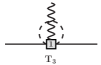
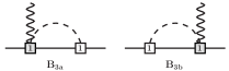
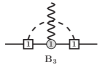
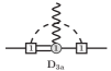
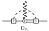
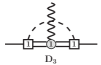
Figure 1: Feynman diagrams contributing up to $\mathcal{O}\left(p^{3}\right)$ to the $g_{1}^{B^{\prime}B}$ AV form factor. Single solid lines denote octet baryons and double lines decuplet baryons. The dashed lines correspond to mesons and the wiggly line to the external AV field. A number inside the vertex denote its chiral order.

For our study, we need the following four terms from the B$\chi$PT Lagrangian

$$\mathcal{L}=\mathcal{L}_{B}^{\left(1\right)}+\mathcal{L}_{B}^{\left(3\right)}+\mathcal{L}_{D}^{\left(1\right)}+\mathcal{L}_{BD}^{\left(1\right)}\,\,\,\,,$$ (6)

where the last two contributions contain the decuplet fields. The number in brackets denotes the chiral order of each part. The first term is the standard leading-order baryon-octet Lagrangian and the second term the $p^{3}$-order part constructed in Oller:2006yh ; Frink:2006hx ; Oller:2007qd . Their explicit expressions are

$$\mathcal{L}_{B}^{\left(1\right)} = \langle\overline{B}\left(i\hbox to0.0pt{\hbox to8.55695pt{\hfil/\hfil}\hss}D-M_{B0}\right)B\rangle+\frac{D}{2}\langle\overline{B}\gamma^{\mu}\gamma_{5}\left\{u_{\mu},B\right\}\rangle+\frac{F}{2}\langle\overline{B}\gamma^{\mu}\gamma_{5}\left[u_{\mu},B\right]\rangle\,\,\,,$$ (7)

$$\mathcal{L}_{B}^{\left(3\right)} = +h_{38}\langle\overline{B}u^{\mu}\gamma_{\mu}\gamma_{5}B\chi_{+}\rangle+h_{39}\langle\overline{B}\chi_{+}\gamma_{\mu}\gamma_{5}Bu^{\mu}\rangle+h_{40}\langle\overline{B}u^{\mu}\gamma_{\mu}\gamma_{5}B\rangle\langle\chi_{+}\rangle+h_{41}\langle\overline{B}\gamma_{\mu}\gamma_{5}Bu^{\mu}\rangle\langle\chi_{+}\rangle$$

$$+h_{42}\langle\overline{B}\gamma_{\mu}\gamma_{5}B\rangle\langle u^{\mu}\chi_{+}\rangle+h_{43}\langle\overline{B}\gamma_{\mu}\gamma_{5}B\left\{u^{\mu},\chi_{+}\right\}\rangle+h_{44}\langle\overline{B}\left\{u^{\mu},\chi_{+}\right\}\gamma_{\mu}\gamma_{5}B\rangle+...\,\,\,\,,$$

where $\langle...\rangle$ denotes the flavor trace and all further notations are explained in App. A. All the LECs in the chiral Lagrangians are formally defined in the chiral limit where, for instance, $M_{B0}$ represents the corresponding baryon mass. At LO, the complete meson-baryon and AV baryon interactions are parametrized by only the two LECs $D$ and $F$. The $\mathcal{L}_{B}^{\left(2\right)}$ does not contain operators that contribute to the AV couplings of the baryons, while several appear at $\mathcal{O}(p^{3})$ that are parameterized by the $h_{i}$ LECs. Note that here we choose the $h_{i}$ with the opposite sign as in Oller:2006yh ; Frink:2006hx ; Oller:2007qd and that only the structures $h_{38,39}$ and $h_{43,44}$ contain explicit $SU(3)$ symmetry breaking terms while the structures $h_{40,41}$ include $SU(3)$-singlets. Finally, the LEC $h_{42}$ does not contribute to SHDs or the isovector couplings (in the isospin limit), although it contributes to the singlet and octet charges of the baryons. We will discuss in Sec. IV.3 the important consequences of this on the interpretation of the proton’s spin.

For the decuplet Lagrangians we use:

$$\mathcal{L}_{D}^{\left(1\right)} = \overline{T}_{\mu}^{abc}\left[\gamma^{\mu\nu\alpha}i\partial_{\alpha}-M_{D0}\gamma^{\mu\nu}\right]T_{\nu}^{abc}-\frac{\mathcal{H}}{2M_{D0}^{2}}\left(\partial_{\sigma}\overline{T}_{\tau}^{abi}\right)\gamma^{\alpha\sigma\tau}u_{\mu}^{ij}\gamma^{\mu}\gamma^{5}\gamma_{\alpha\kappa\lambda}\left(\partial^{\kappa}T^{abj\,\lambda}\right)\,\,\,\,,$$ (8)

$$\mathcal{L}_{DB}^{\left(1\right)} = \frac{i\mathcal{C}}{M_{D0}}\left[\left(\partial_{\mu}\overline{T}_{\nu}^{ijk}\right)\gamma^{\mu\nu\lambda}u_{\lambda}^{jl}B^{km}+\overline{B}^{mk}\gamma^{\mu\nu\lambda}u_{\lambda}^{lj}\left(\partial_{\mu}T_{\nu}^{ijk}\right)\right]\varepsilon^{ilm}\,\,\,\,,$$ (9)

where $X^{ab}$ denotes the matrix element in the $a$-th row and $b$-th column. Each entry of the totally symmetric tensor $T^{abc}$ is a spin-3/2 Rarita-Schwinger spinor representing a decuplet baryon. In App. A we define explicitly all relevant quantities. The $\mathcal{C}$ and $\mathcal{H}$ are the AV octet-decuplet and decuplet couplings, respectively, and $M_{D0}$ is the chiral-limit decuplet baryon mass. In the case of $\mathcal{C}$, our definition differs by a factor of $2$ as compared to the large $N_{c}$ work Dashen:1994qi .

The above decuplet Lagrangians implement the consistent couplings of Pascalutsa:1998pw ; Pascalutsa:1999zz ; Pascalutsa:2000kd . They are consistent in the sense that the invariance of the free theory under a decuplet field redefinition of $\Psi^{\mu}\to\Psi^{\mu}+\partial^{\mu}\epsilon\left(x\right)$, with $\epsilon\left(x\right)$ a spinor field, carries over to the interacting theory. This ensures the decoupling of the spurious spin-1/2 components of the Rarita-Schwinger spinor. In this way we also obtained the last term in Eq. (8), i.e. by substituting $\Psi^{\mu}\to\left(i/M_{D0}\right)\gamma^{\mu\alpha\nu}\left(\partial_{\alpha}\Psi_{\nu}\right)$ Pascalutsa:2006up in the non-consistent Lagrangian

$$\mathcal{L}_{nc}^{\left(1\right)}=\frac{\mathcal{H}}{2}\overline{T}_{\alpha}^{abi}u_{\mu}^{ij}\gamma^{\mu}\gamma^{5}T^{abj\,\alpha}\,\,\,.$$ (10)

With the above Lagrangians, we can now write down all terms that contribute up to order $p^{3}$ to the AV charges $g_{1}^{B^{\prime}B}$ and $g_{A,3}^{BB}$. The full unrenormalized result in dimensional regularization is

$$g_{X}^{B^{\prime}B} = \sqrt{Z_{B^{\prime}}}\sqrt{Z_{B}}C_{1}^{B^{\prime}B}+C_{3}^{B^{\prime}B}+T_{3}^{B^{\prime}B}+B_{3}^{B^{\prime}B}+B_{3ab}^{B^{\prime}B}+D_{3}^{B^{\prime}B}+D_{3ab}^{B^{\prime}B}+\mathcal{O}\left(p^{4}\right)\,\,\,\,,$$ (11)

where the notation matches the one of Fig. 1 and we list all contributions explicitly in App. B. The factors $Z_{B}$ are the wavefunction-renormalization constants which, at this order, only contribute through the LO terms. Furthermore, we apply the EOMS renormalization scheme Gegelia:1999gf ; Fuchs:2003qc at a scale $\Lambda=\overline{M}_{B}$.

We use Eq. (11) to fit in Sec. IV the data of Tab. 1. Some of the LECs appearing in the loop functions are already well constrained by other observables than the AV charges and we will use this additional information. Explicitly, these are the meson decay constant $f_{0}$, the baryon masses $M_{B0}$ and $M_{D0}$, and the couplings of the decuplet $\mathcal{C}$ and $\mathcal{H}$, all in the chiral limit. The former three can be determined using the extrapolation of lQCD data, namely, $f_{0}\simeq 87$ MeV Aoki:2013ldr , $M_{B0}\simeq 880$ MeV Ren:2012aj and $M_{D0}\simeq 1152$ MeV Ren:2013dzt . The decuplet couplings in the chiral limit are not well known and we use the Large $N_{c}$ relations $\mathcal{C}=-D$ and $\mathcal{H}=3D-9F$ Dashen:1994qi , which are valid up to $1/N_{c}^{2}$ corrections.

However, one can also use an alternative set for these parameters based on their experimental values which are better known. In this case, $f_{0}=\overline{f}$, $M_{0}=\overline{M}_{B}$ and $M_{D0}=\overline{M}_{D}$, where $\overline{f}$ is the average of physical pion, kaon and $\eta$-decay constants and $\overline{M}_{B\left(D\right)}$ the average of the physical baryon masses in the respective multiplet. The octet-decuplet coupling is determined from the (strong) decuplet decays to $\mathcal{C}=-0.85(15)$. The experimental decuplet coupling $\mathcal{H}$ is not known and we use again the large $N_{c}$ relation.

In Tab. 2 we list the input parameters used in each case. Note that both choices are equivalent as one can rewrite one into the other at the expense of higher order contributions. We will perform our analysis with these two sets of values in order to assess systematic uncertainties.

As a final remark concerning the determination of $D$ and $F$ at $\mathcal{O}(p^{3})$, we note that the LECs $h_{40,41}$ have the same structure as the LO couplings but come multiplied by a singlet of quark masses. We introduce lQCD results on the AV couplings in our statistical analysis precisely to disentangle these LECs from the $D$ and $F$.

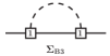
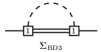
Figure 2: Diagrams contributing to the wave-function renormalization. The notation is the same as in Fig. 1.

Table 2: Values of low-energy constants fixed in our fits. We list the meson decay constant $f_{0}$, the pion, kaon and $\eta$ masses $M_{\pi},$ $M_{K}$ and $M_{\eta}$, and the octet and decuplet masses $M_{B0}$ and $M_{D0}$, respectively. As described in the text, we use two perturbatively equivalent sets for the explicit numerical values entering the fits.

appearing quantity	$f_{0}$ [MeV]	$M_{\pi}$ [MeV]	$M_{K}$ [MeV]	$M_{\eta}$ [MeV]	$M_{B0}$ [MeV]	$M_{D0}$ [MeV]	$\mathcal{C}$	$\mathcal{H}$
chiral limit choice	$87$	$140$	$496$	$547$	$880$	$1152$	$-D$	$3D-9F$
physical average choice	$1.17\cdot 92$	$140$	$496$	$547$	$1149$	$1381$	$-0.85$	$3D-9F$

IV Results

In this section we analyze the SHD data and the lQCD results described in Sec. II and listed in Tab. 1. We use the covariant B$\chi$PT in the EOMS scheme Gegelia:1999gf ; Fuchs:2003qc up to $\mathcal{O}(p^{3})$, which leads to Eq. (11) for the octet-baryon AV charges. In its complete form, there are eight fitted LECs appearing: $D,$ $F$, $h_{38-41,43,44}$. The Tab. 1 contains updated experimental data as compared to the ones used in previous works. We start discussing earlier results obtained in analyses done at LO in the chiral expansion or at NLO in the HB$\chi$PT or IR-B$\chi$PT approaches.

IV.1 Leading order results and previous NLO B$\chi$PT analyses

We examine first the description of the data at leading order in B$\chi$PT, i.e. to $\mathcal{O}(p)$. This is equivalent to the $SU(3)$-symmetric Cabibbo model Cabibbo:1963yz ; Cabibbo:2003cu and the fits are shown in Tab. 3. We approximately reproduce the results of Cabibbo:2003cu , taking into account the updated SHD data and also excluding the $\Sigma^{-}\to\Lambda$ channel. Its consideration worsens the LO fit as it produces the highest contribution to the $\chi^{2}$. However, in the next section we will see that the description improves at NLO. For illustration, we also include the lQCD data in one of the fits. This gives similarly good results, which already indicates that the quark-mass dependence of the AV charges is moderate. Additionally, this suggests that the interpretation given in Cabibbo:2003cu that there are only mild $SU(3)$ breaking effects in SHD carries also over to unphysical quark masses. We will discuss this later in more detail.

Table 3: Cabibbo model fits to the SHD data. The leading order B$\chi$PT is equivalent to the Cabibbo model. In the second column we use the old data of Cabibbo:2003cu and in the others the data of Tab. 1 where the $\Xi^{0}\to\Sigma^{+}$ mode is updated AlaviHarati:2001xk ; Batley:2006fc and the $\Sigma^{-}\to\Lambda$ one is included.

	Cabibbo:2003cu	SHD	SHD+lQCD
$D$	$0.804(8)$	$0.800(8)$	$0.785(5)$
$F$	$0.463(8)$	$0.469(8)$	$0.483(5)$
$F/D$	$0.58$	$0.59$	$0.62$
$\chi_{\mbox{red}}^{2}$	$\frac{2.0}{3}=0.7$	$\frac{13.6}{3}=4.5$	$\frac{23.5}{17}=1.4$

At NLO there are several works on the AV charges in HB$\chi$PT Jenkins:1990jv ; Jenkins:1991es ; Savage:1996zd . Many more studies implement a combined chiral and $1/N_{c}$ expansion that aims at exploiting the cancellations between octet and decuplet loop diagrams arising in the Large $N_{c}$ limit Dashen:1993as ; Dashen:1993jt ; Dashen:1994qi ; FloresMendieta:2000mz ; FloresMendieta:2012dn ; CalleCordon:2012xz . Here we will restrict ourselves to the discussion of the previous analyses of the chiral expansion of $g_{1}(0)$.

The HB results can be obtained by keeping only the LO term of a (non-relativistic) expansion of the covariant loop-functions in powers of $1/M_{B}$. We have checked that we recover all the non-analytic structures reported in these earlier HB works, including those concerning the decuplet contributions in the SSE FloresMendieta:2000mz . The main difference of these studies with respect to ours is that all the contributions from analytic parts were neglected. That is, those stemming from the loop contributions were removed and $h_{i}=0$ was assumed, as well as the approximations $\Delta=M_{D0}-M_{B0}=0$ and $M_{\pi}=0$ were employed. To account for all this, the errors of the SHD data were increased globally to $0.2$. In using these same approximations and the data of Tab. 1, we are able to qualitatively reproduce the results and conclusions of Jenkins:1990jv ; Jenkins:1991es .

In any case, this treatment of NLO corrections and the increment of error bars is not systematic. In particular, we will see below that the role of the analytic terms is very important and they are a source for cancellations at NLO that dominate those between the octet and the decuplet.

Apart from the HB studies, the work in IR-B$\chi$PT of Ref. Zhu:2000zf correctly incorporated the $\mathcal{O}(p^{3})$ contact terms, i.e. included all the LECs $h_{i}$. To perform fits, the two $SU(3)$ symmetric LECs $h_{40/41}$ are absorbed into $D$ and $F$, leading to the same number of fit-parameters as of input data. They specifically investigated the effect of the leading recoil corrections in the IR-B$\chi$PT, and found that these, which formally are of $\mathcal{O}(p^{4})$ in the HB expansion, are typically larger than the LO ones. Naturally, the conclusion of this study was that the convergence of the chiral expansion of $g_{1}(0)$ is severely broken.

However, this work has some weaknesses that need to be scrutinized. Firstly, the fitted parameters $D$ and $F$ are not those defined in the chiral limit but an effective parametrization which mixes $\mathcal{O}(p)$ and $\mathcal{O}(p^{3})$ contributions. This hinders any definite discussion about the convergence of the chiral expansion of $g_{1}(0)$. Secondly, the decuplet contributions are neglected despite of the important role they play in reducing the overall size of the loop corrections, as suggested by the previous HB and Large $N_{c}$ studies. Finally, and most importantly, it must be investigated if the large size of the recoil corrections reported in this paper, which are roughly a factor 10 larger than expected by power counting, is a genuine problem of the chiral expansion or, instead, an artifact introduced by the IR renormalization scheme. In the next section, we discuss our complete results in the EOMS scheme where we tackle all the issues mentioned above.

IV.2 Results in the EOMS-B$\chi$PT at NLO

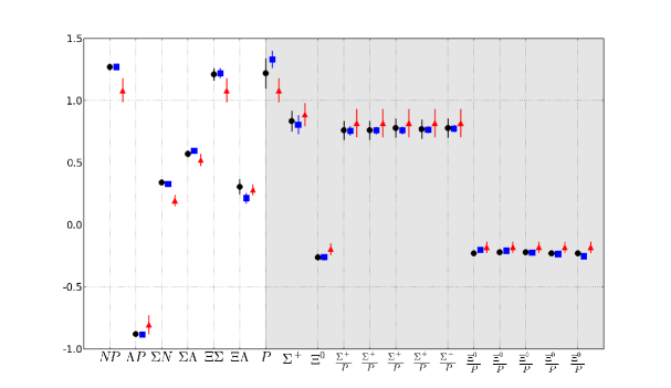
Figure 3: Axial-vector charges $g_{1}^{BB^{\prime}}$ and $g_{A,3}^{X}$ of the SHD and octet baryons compared to our fits including explicit virtual decuplet states. Blue circle markers denote the fitted input data points. The square markers denote our full B$\chi$PT results while the triangle markers show the LO contribution. The shaded area corresponds to the lQCD input from Lin:2007ap and Gockeler:2011ze . In the case of the lQCD data from Gockeler:2011ze , the data points are listed from left to right with increasing $M_{\pi}$.

In Tab. 4 and Fig. 3, we show our final results of the EOMS-B$\chi$PT fits to the SHD data and lQCD results discussed in Sec. II. The description is excellent at NLO whether decuplet resonances are explicitly included or not. Also, the $\Sigma^{-}\to\Lambda$ mode can now be consistently described.

For each channel and fit strategy, we separate the different contributions to $g_{1}(0)$. By looking at the last row in Tab. 5, it can be noticed that the total NLO contribution is typically smaller than $20\%$ ($30\%$) of the LO one, except for the $\Sigma^{-}\to n$ channel which could be up to a $\sim 68\%$ ($\sim 118\%$) in the theory with (without) explicit decuplets. The overall picture is consistent with the naive power counting by which one expects the $\mathcal{O}(p^{3})$ corrections to be around $(M_{k}/\Lambda)^{2}\sim 25\%$ of the $\mathcal{O}(p)$ ones.

As a consequence, B$\chi$PT at NLO is compatible with small $SU(3)$-breaking effects in the SHD. This is remarkable since only at LO the Lagrangian is fully $SU(3)$ symmetric and most NLO operators or loop corrections break the symmetry. This structure, together with the actual number of LECs, is not arbitrary but dictated by spontaneous chiral symmetry breaking and chiral power counting. In practice, the successful description of the SHD data and the good convergence are achieved by sizable cancellations between the different NLO terms. These cancellations are different in the theories with or without the explicit decuplet baryons.

In the theory without the decuplet, the loop contributions are given by the tadpoles ($T_{3}$) and the diagrams with internal octet baryons ($B^{loops}$) only. Individually, these are typically $25\%$ of the LO value although they can be as large as a $50\%$. On top of that, they have the same sign in almost all the channels. The large $SU(3)$-breaking thus produced is not compatible with the SHD data and, as a result, the LECs $h_{i}$ coming from the $\mathcal{O}(p^{3})$ contact-terms ($C_{3}$) are adjusted in the fit to largely cancel the effects of the loops.

On the other hand, in the theory with explicit decuplet contributions, the new loops ($D^{loops}$) can be as sizable as the other ones but, generally, with the opposite sign. We observe that the octet-decuplet cancellations found in Jenkins:1991es carry over to the covariant formulation of B$\chi$PT and using a finite octet-decuplet mass splitting. The main consequence of this is an important reduction of the net contribution of the loops and, hence, of the size of the $C_{3}$ terms. Although the results and overall convergence patterns look equivalent in both theories, the inspection of the different pieces reveals that the values of the LECs in the theory with the decuplet are more natural.

In Tab. 5 we show the values of our fitted parameters. As discussed in Sec. III, one has the freedom at NLO to fix some the LECs to either their chiral limit values or the average of their physical ones. Our default choice is the latter, which corresponds to the results of Tab. 4. However, we list the values of the fitted LECs for both choices and notice that the results are rather insensitive with respect to these sets of input parameters. We also tested the impact of the decuplet LEC $\mathcal{H}$ when allowing for a $10\%\sim 1/N_{C}^{2}$ uncertainty to the large-$N_{C}$ input or fixing it by the $SU(2)$ relation $\mathcal{H}=-g_{A}(8/5)$. In all cases we obtain results that are compatible within the statistical uncertainties of those given in Tabs. 4 and 5.

In the last row of Tab. 5 we show the reduced $\chi^{2}$ for the different fits. By comparing them to those from the LO fits in Tab. 3, one notes that the description of the data improves at NLO. The values of $D$ and $F$ change by $\sim 21\%$ and $\sim 6\%$, respectively. Furthermore, it is remarkable that at NLO the ratio $F/D$ is closer to its Large $N_{c}$ prediction of $2/3$. As for the $\mathcal{O}(p^{3})$ LECs, there are large differences between the results in the theory with or without the decuplet. This is expected on general grounds since the effects of the resonances are encoded in the values of the LECs in the latter case.

As a final result for $D$ and $F$ we report

$$D=0.623(61)(17),\hskip 85.35826ptF=0.441(47)(2),$$ (12)

which is the average between our results with explicit decuplets as listed in Tab. 5. This accounts for the “naturalness” issue we addressed above for the decuplet-less theory and the fact that integrating out decuplet resonances in a $SU(3)$ context is not well justified. The first error is statistical and the second a systematical one, that covers the central values of the two fits. As an interesting by-product of our results, we predict the chiral-limit value of $g_{A0}=1.064(77)(19)$ in the $SU(3)$-B$\chi$PT, which is smaller than the physical AV charge of $g_{A}=1.270(3)$.

Having obtained a reliable description of the $g_{1}/f_{1}$ ratios of the SHD, we are also able to discuss the channels that did not enter in our fits. These are the SHDs $\Sigma^{-}\to\Sigma^{0}$ and $\Xi^{-}\to\Xi^{0}$ and the isovector AV charges $g_{A,3}^{\Sigma^{{}_{+}}\Sigma^{{}_{+}}}$ and $g_{A,3}^{\Xi^{0}\Xi^{0}}$ at the physical point. They are not experimentally measured yet and our values are predictions. We list the results in the last four columns of Tab. 4. Note that the values shown for the SHD and the charges are related by isospin. However, for convenience we give both of them explicitly.

Since we can apply a non-relativistic expansion to our covariant formulas, we are also able to perform a similar SHD study in the HB formalism. We list the results for the decuplet-less case in App. C. Also with this approach, we obtain an excellent description of the SHD data with equivalent conclusions to those discussed above. These findings, together with our EOMS results above, are quite the opposite to those in the covariant IR-B$\chi$PT study Zhu:2000zf where very large recoil corrections are reported. As a result, we conclude that the stated poor chiral convergence might be related to the problems this covariant prescription introduces in the analytic structure of the loop functions Geng:2008mf ; Ledwig:2010nm ; Ledwig:2011cx ; Alarcon:2012kn . Apart from this, we want to stress that the agreement between covariant and HB$\chi$PT is quite remarkable given the sizable differences that have been found between these approaches in other $SU(3)$-B$\chi$PT applications Geng:2008mf ; Geng:2009hh ; MartinCamalich:2010fp . Probably this is a consequence of the large number of LECs at NLO, as it can be seen by comparing the values in the different columns. Differences between the two approaches might show up in other observables where the values of these LECs also appear, e.g. in meson-baryon scattering processes.

Table 4: Axial-vector charges and couplings of the octet baryons. We used the average of the physical values for the fixed LECs. The results are decomposed into their chiral order contributions, i.e. into LO and the individual $p^{3}$ contributions of the graphs $C_{3}$, $T_{3}$ and loops with virtual octet baryons $B^{loops}$ or decuplet baryons $D^{loops}$. We also show the total NLO contributions relative to the LO one. In the last four columns are predictions for the strangeness-conserving SHD where the values of $g_{1}^{BB^{\prime}}$ and $g_{A,3}^{B}$ are connected by isospin symmetry.

$g_{1}$	$N\to P$	$\Lambda\to P$	$\Sigma^{-}\to n$	$\Sigma^{-}\to\Lambda$	$\Xi^{0}\to\Sigma^{+}$	$\Xi^{-}\to\Lambda$	$\Sigma^{-}\to\Sigma^{0}$	$\Xi^{-}\to\Xi^{0}$	$g_{A,3}^{\Sigma^{+}}$	$g_{A,3}^{\Xi^{0}}$
Exp	$1.270(3)$	$-0.879(18)$	$0.340(17)$	$0.570(27)$	$1.210(50)$	$0.306(61)$	na	na	na	na
Cov
LO	$1.16$	$-0.89$	$0.15$	$0.54$	$1.16$	$0.35$	$0.72$	$0.15$	$1.01$	$-0.150$
$C_{3}$	$-0.45$	$0.59$	$0.14$	$-0.30$	$-0.92$	$-0.49$	$-0.50$	$-0.01$	$-0.71$	$0.01$
$T_{3}$	$0.27$	$-0.40$	$0.07$	$0.13$	$0.52$	$0.16$	$0.17$	$0.04$	$0.24$	$-0.04$
$B^{loops}$	$0.29$	$-0.19$	$-0.03$	$0.23$	$0.45$	$0.22$	$0.34$	$0.02$	$0.48$	$-0.02$
full	$1.270(3)$	$-0.886(18)$	$0.327(15)$	$0.597(22)$	$1.213(38)$	$0.240(41)$	$0.718(52)$	$0.201(38)$	$1.016(74)$	$-0.201(38)$
$|p^{3}/p^{1}|$	$0.09$	$\sim 0.0$	$1.18$	$0.11$	$0.04$	$0.32$	$\sim 0$	$0.33$	$\sim 0$	$0.33$
Cov+D
LO	$1.08$	$-0.80$	$0.20$	$0.52$	$1.08$	$0.28$	$0.62$	$0.20$	$0.89$	$-0.20$
$C_{3}$	$-0.18$	$0.24$	$0.01$	$-0.18$	$-0.28$	$-0.17$	$0.08$	$-0.22$	$0.11$	$0.22$
$T_{3}$	$0.25$	$-0.36$	$0.09$	$0.12$	$0.48$	$0.13$	$0.15$	$0.05$	$0.21$	$-0.05$
$B^{loops}$	$0.18$	$-0.09$	$-0.02$	$0.17$	$0.30$	$0.12$	$0.24$	$0.06$	$0.34$	$-0.06$
$D^{loops}$	$-0.07$	$0.13$	$0.06$	$-0.03$	$-0.37$	$-0.15$	$-0.36$	$0.15$	$-0.51$	$-0.15$
full	$1.270(3)$	$-0.883(18)$	$0.330(16)$	$0.597(22)$	$1.221(40)$	$0.214(42)$	$0.740(55)$	$0.225(35)$	$1.047(77)$	$-0.225(35)$
$|p^{3}/p^{1}|$	$0.17$	$0.10$	$0.68$	$0.14$	$0.13$	$0.24$	$0.18$	$0.15$	$0.18$	$0.15$

Table 5: Fit results of our EOMS B$\chi$PT analysis of the data in Tab. 1. In the large $N_{C}$ limit one has $F/D=2/3$ and $\mathcal{C}=-D$. We list the results with respect to the choices of fixed parameters as shown in Tab. 2. The choice of chiral limit parameters is marked with chiral.

	Cov	Cov+D	Cov chiral	Cov+D chiral
$D$	$0.658(64)$	$0.639(61)$	$0.634(59)$	$0.606(53)$
$F$	$0.507(56)$	$0.443(47)$	$0.492(52)$	$0.439(42)$
$F/D$	$0.77$	$0.69$	$0.78$	$0.72$
$h_{38}$ [GeV-2]	$0.146(29)$	$-0.008(34)$	$0.143(27)$	$-0.051(37)$
$h_{39}$ [GeV-2]	$-0.002(36)$	$0.032(36)$	$0.006(38)$	$0.049(42)$
$h_{40}$ [GeV-2]	$-0.349(135)$	$-0.077(102)$	$-0.354(133)$	$-0.030(52)$
$h_{41}$ [GeV-2]	$-0.009(47)$	$-0.151(49)$	$-0.004(45)$	$-0.113(59)$
$h_{43}$ [GeV-2]	$0.082(39)$	$0.159(49)$	$0.083(39)$	$0.159(53)$
$h_{44}$ [GeV-2]	$-0.111(26)$	$-0.062(22)$	$-0.118(25)$	$-0.062(15)$
$\chi_{\mbox{red}}^{2}$	$\frac{7.0}{11}=0.64$	$\frac{7.4}{11}=0.67$	$\frac{7.2}{11}=0.65$	$\frac{7.9}{11}=0.72$

Finally, we are also able to discuss how the $SU(3)$-breaking effects behave for unphysical quark-masses. In Figs. 4 and 5 we show the chiral behavior of the isovector AV charges as function of $M_{\pi}$, together with the ratios of the NLO contributions over the LO ones, i.e. their chiral convergences. We also plot the LO contributions of the NLO fits as well as the results of the pure Cabibbo model fits (LO B$\chi$PT) of Sec. 3.

We see that the chiral behavior is quite flat and is in very good agreement with the LO result and the dependence shown by the lQCD studies. Therefore, the cancellations among various $p^{3}$ terms at the physical point also hold for unphysical quark masses. The overall chiral convergence is very acceptable for the whole quark-mass region. Similar chiral extrapolations can be found in the theory without explicit decuplet states as well as in the HB approach.

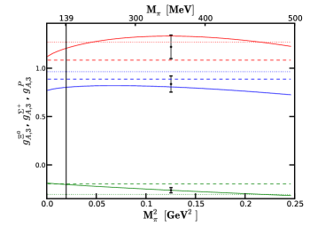
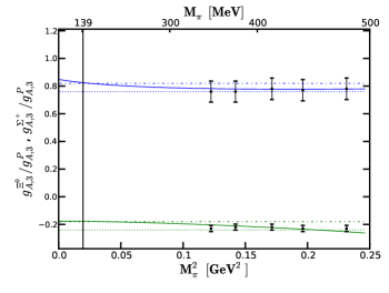
Figure 4: Chiral extrapolation of the AV charges $g_{A,3}^{X}$ of the proton (red), $\Sigma^{+}$ (blue) and $\Xi^{0}$ (green) as function of $M_{\pi}$. The left figure shows the lowest $M_{\pi}$ data from Lin:2007ap with $M_{k}=604$ MeV. The right figure shows the data from Gockeler:2011ze along the $SU(3)$ singlet line for $g_{A,3}^{\Sigma^{+}}/g_{A,3}^{P}$ (blue) and $g_{A,3}^{\Xi^{0}}/g_{A,3}^{P}$ (green). We also plot the LO contribution as obtained from the full $p^{3}$ fit, dashed line, as well as the LO results of Sec. IV.1, dotted line.

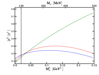
Figure 5: Chiral convergence of the AV charges. We show the ratio of NLO contributions over the LO one for the $g_{A,3}^{X}$ of the proton (red), $\Sigma^{+}$ (blue) and $\Xi^{0}$ (green) as function of $M_{\pi}$.

IV.3 Octet axial-vector charges and the quark contribution to the proton’s spin

A very important application of the study of the SHDs has been the prediction of the octet axial charge of the proton, $g_{A}^{8}$. This is defined as the axial charge corresponding to $\langle P(p^{\prime})|\overline{q}\gamma^{\mu}\gamma_{5}\lambda^{8}q|P(p^{\prime})\rangle$ and its importance lies on the fact that it gives a crucial constraint to obtain the flavor structure of the quark contribution to the proton’s spin (see Aidala:2012mv for a recent review). Even though this is an old and persisting question in nucleon structure, the value of $g_{A}^{8}$ is not well known yet. At LO in the chiral expansion one recovers the $SU(3)$ prediction that $g_{A}^{8}=3F-D\simeq 0.58$. The success of the Cabibbo model in the description of the SHDs suggests that this determination could be accurate and it is often used in the phenomenological analyses. However, a model-independent understanding of the quark contribution to the proton spin requires a better determination of $g_{A}^{8}$ and efforts in this direction have been undertaken in lQCD QCDSF:2011aa ; Engelhardt:2012gd .

In principle, B$\chi$PT can be used to improve the determination to higher orders in the chiral expansion. Such studies were carried out in the HB Jenkins:1990jv and IR Zhu:2000zf schemes and the conclusions were in both cases that the NLO correction could be very large which hampered the convergence of the chiral expansion of $g_{A}^{8}$. However, these conclusions are afflicted by the same caveats as those addressed above in Sec. IV.1, and they should be revised in the context of the current full NLO calculation. Furthermore, the octet axial charge receives a contribution from a LEC, $h_{42}$, that is not constrained by SHDs data as it does not contribute to the flavor-changing transitions or to the isospin related isovectorial charges. This fact has been overlooked in the previous chiral analyses and it precludes a determination of $g_{A}^{8}$ from SHDs alone.

Table 6: Different contributions to $g_{A}^{8}$ in EOMS-B$\chi$PT up to $\mathcal{O}(p^{3})$ and assuming $g_{A}^{8}=0.58$.

	LO	NLO	$C_{3}$	$T_{3}$	$B_{3}$	$D_{3}$
Octet	0.84	$-0.26$	$-0.72$	0.55	$-0.09$	$-$
Octet+Decuplet	0.71	$-0.13$	$-0.38$	0.47	$-0.13$	$-0.09$

Nevertheless, even without a precise value for $h_{42}$ we are able to study the convergence of $g_{A}^{8}$ under quite general assumptions. For this, we assume that $g_{A}^{8}$ is close to its $SU(3)$-symmetric value, $g_{A}^{8}\sim 0.58$, as suggested by a recent lQCD determination, and we fix $h_{42}$. The size of the different contributions up to $\mathcal{O}(p^{3})$ are shown in Tab. 6. By comparing the overall LO and NLO contributions, we see that the convergence in this scenario is good, with NLO corrections about a 20% (30%) the LO ones in the decuplet (decuplet-less) theory. In the theory without decuplets one finds that the total loop contribution is quite large. As a consequence, the NLO contact-terms are sizable and as large as the total LO. This leads to the same naturalness considerations discussed above for the AV charges. On the other hand, the diagrams with decuplet baryons reduce the net loop contribution and improve the convergence.

The current analysis clarifies the structure of the chiral expansion of the octet axial coupling of the proton and opens the possibility for a model-independent treatment of its $SU(3)$-breaking corrections and for an improvement of the phenomenological extractions of the quark content of the proton’s spin.

V Summary

We have studied the axial-vector charges of the octet baryons in $SU(3)$ covariant B$\chi$PT up to $\mathcal{O}(p^{3})$ using the EOMS scheme and including decuplet resonances. We report that B$\chi$PT at this next-to-leading order consistently describes the charges as well as the ratios $g_{1}/f_{1}$ of the axial-vector and vector couplings measured in the semileptonic hyperon decays. This is a novel feature as compared with previous B$\chi$PT studies in the non-relativistic heavy-baryon scheme or the relativistic infrared approach.

Explicitly, we have been able to determine all appearing low-energy constants from simultaneous fits to the semileptonic hyperon decay data and available lQCD results. This includes the leading-order constants $D$ and $F$ as well as all the NLO constants $h_{38-41,43,44}$. Along this, we have clarified the role of the different contact-terms appearing at this order which were not treated systematically in the previous works. Especially, we disentangle the two singlet LECs $h_{40,41}$ from $D$ and $F$, which lead to an accurate determination of the latter and a consistent discussion of the chiral convergence for the axial-vector charges.

We report a systematic improvement of the theoretical understanding of the data with respect to the $SU(3)$-symmetric Cabibbo model, which is equivalent to the B$\chi$PT at LO. That is, at NLO we are also able to consistently include the mode $\Sigma^{-}\to\Lambda$, as well as we obtain NLO corrections that are typically 20% of the LO ones. This size of NLO effects is in agreement with the naive power counting. Therefore, our analysis shows that $SU(3)$-symmetry-breaking effects, as given by the spontaneous chiral symmetry and the chiral power counting in B$\chi$PT, are important to understand the SHD data accurately.

In practice, the agreement at $\mathcal{O}(p^{3})$ is achieved by sizable cancellations between different $SU(3)$ breaking terms, in particular those parameterized by the NLO LECs $h_{i}$ and the ones from the loops. We showed that considering only NLO non-analytic terms is not enough and that NLO analytic terms play an important role. The cancellations themselves appear in both theories with and without explicit decuplet states, however, they have a different structure. In the case with decuplet baryons, we found that their explicit contributions are a source of cancellations which lead to more natural values for the NLO LECs. This is in agreement with the expectations derived from the analysis at large $N_{c}$. Furthermore, the fact that in the decuplet-theory we can successfully describe the small $SU(3)$-breaking in $g_{1}(0)$ by means of a chiral expansion without anomalously large or small chiral corrections at NLO is a very non-trivial outcome of our study.

A phenomenological consequence of our work is the determination of the LO axial couplings $D=0.623(61)(17)$ and $F=0.441(47)(2)$ up to $\mathcal{O}(p^{3})$ accuracy in a completely systematic fashion. Remarkably, these values are closer to the Large $N_{c}$ ratio $D/F\sim 2/3$ than at LO and they predict the axial coupling of the nucleon in the chiral limit and in $SU(3)$ to be $g_{A0}=1.064(77)(19)$. We also predict the isovector axial-vector charges for the $\Lambda$, $\Sigma^{+}$ and $\Xi^{0}$ or, equivalently, for the SHD channels of $\Sigma^{-}\to\Sigma^{0}$ and $\Xi^{-}\to\Xi^{-}$.

Finally, we have discussed an important application of the analysis of the axial-vector charges, namely the prediction of the octet axial coupling $g_{A}^{8}$ and its role in the determination of the quark content of the proton spin. More specifically, we have found that there is a contribution from a NLO contact-term (whose LEC is labelled by $h_{42}$) which is unconstrained by SHDs. Therefore one needs additional experimental or nonperturbative information to determine this parameter. Nevertheless, we studied the chiral convergence of $g_{A}^{8}$ and concluded that it is reasonable. This should allow for a model independent determination of this quantity.

Appendix A Notation

The notation for the baryon Lagrangian Eq. (6) is as follows.
The meson field $\phi=\phi(x)$ is defined by

$$U = e^{i\frac{\sqrt{2}}{f_{0}}\phi}\,\,\,\,\mbox{and}\,\,\,\,u=\sqrt{U}$$ (13)

$$\phi = \frac{\lambda^{a}\phi^{a}}{\sqrt{2}}=\frac{1}{\sqrt{2}}\left[\begin{array}[]{ccc}\phi^{3}+\frac{1}{\sqrt{3}}\phi^{8}&\phi^{1}-i\phi^{2}&\phi^{4}-i\phi^{5}\\ \phi^{1}+i\phi^{2}&-\phi^{3}+\frac{1}{\sqrt{3}}\phi^{8}&\phi^{6}-i\phi^{7}\\ \phi^{4}+i\phi^{5}&\phi^{6}+i\phi^{7}&-\frac{2}{\sqrt{3}}\phi^{8}\end{array}\right]=\left[\begin{array}[]{ccc}\frac{1}{\sqrt{2}}\pi^{0}+\frac{1}{\sqrt{6}}\eta&\pi^{+}&K^{+}\\ \pi^{-}&-\frac{1}{\sqrt{2}}\pi^{0}+\frac{1}{\sqrt{6}}\eta&K^{0}\\ K^{-}&\overline{K}^{0}&-\frac{2}{\sqrt{6}}\eta\end{array}\right]\,\,\,.$$ (20)

The octet baryon field $B\left(x\right)$ is defined by

$$B=\frac{\lambda_{a}}{\sqrt{2}}B_{a} = \left[\begin{array}[]{ccc}\frac{1}{\sqrt{2}}\Sigma^{0}+\frac{1}{\sqrt{6}}\Lambda&\Sigma^{+}&p\\ \Sigma^{-}&-\frac{1}{\sqrt{2}}\Sigma^{0}+\frac{1}{\sqrt{6}}\Lambda&n\\ \Xi^{-}&\Xi^{0}&-\frac{2}{\sqrt{6}}\Lambda\end{array}\right]=\left(B^{ab}\right)\,\,\,\,,$$ (24)

$$\overline{B}=\frac{\lambda_{a}}{\sqrt{2}}\overline{B}_{a} = \left[\begin{array}[]{ccc}\frac{1}{\sqrt{2}}\overline{\Sigma}^{0}+\frac{1}{\sqrt{6}}\overline{\Lambda}&\overline{\Sigma}^{-}&\overline{\Xi}^{-}\\ \overline{\Sigma}^{+}&-\frac{1}{\sqrt{2}}\overline{\Sigma}^{0}+\frac{1}{\sqrt{6}}\overline{\Lambda}&\overline{\Xi}^{0}\\ \overline{p}&\overline{n}&-\frac{2}{\sqrt{6}}\overline{\Lambda}\end{array}\right]=\left(\overline{B}^{ab}\right)\,\,\,\,.$$ (28)

The decuplet field $T\left(x\right)$ is defined by the totally symmetric tensor $T^{abc}$

$$T_{111}^{\alpha}=\Delta^{++\alpha}\,\,\,\,T_{112}^{\nu}=\frac{1}{\sqrt{3}}\Delta^{+\alpha} T_{122}^{\alpha}=\frac{1}{\sqrt{3}}\Delta^{0\alpha}\,\,\,\,T_{222}^{\alpha}=\Delta^{-\alpha}$$ (29)

$$T_{113}^{\nu}=\frac{1}{\sqrt{3}}\Sigma^{*+\alpha} \,\,\,\,T_{123}^{\nu}=\frac{1}{\sqrt{6}}\Sigma^{*0\alpha}\,\,\,\, T_{223}^{\alpha}=\frac{1}{\sqrt{3}}\Sigma^{*-\alpha}$$ (30)

$$T_{133}^{\nu}=\frac{1}{\sqrt{3}}\Xi^{*0\alpha} T_{233}^{\alpha}=\frac{1}{\sqrt{3}}\Xi^{*-\alpha}\,\,\,\,$$ (31)

$$T_{333}^{\alpha}=\Omega^{-\alpha} \,\,\,\,,$$ (32)

together with the decuplet baryon propagator as

$$S_{\Delta}^{\alpha\beta}(p)=\frac{\hbox to0.0pt{\hbox to5.03125pt{\hfil/\hfil}\hss}p+M_{D0}}{p^{2}-M_{D0}^{2}+i\varepsilon}\left[-g^{\alpha\beta}+\frac{1}{D-1}\gamma^{\alpha}\gamma^{\beta}+\frac{1}{(D-1)M_{D0}}(\gamma^{\alpha}p^{\beta}-\gamma^{\beta}p^{\alpha})+\frac{D-2}{(D-1)M_{D0}^{2}}p^{\alpha}p^{\beta}\right]\,\,\,.$$ (33)

The external axial-vector field is defined by

$$a_{\mu}=a_{\mu}^{a}\left(x\right)\frac{\lambda^{a}}{\sqrt{2}}=\left[\begin{array}[]{ccc}\frac{1}{\sqrt{2}}a^{0}+\frac{1}{\sqrt{6}}a^{\eta}&a^{\pi^{+}}&a^{K^{+}}\\ a^{\pi^{-}}&-\frac{1}{\sqrt{2}}a^{0}+\frac{1}{\sqrt{6}}a^{\eta}&a^{K^{0}}\\ a^{K^{-}}&a^{\overline{K}^{0}}&-\frac{2}{\sqrt{6}}a^{\eta}\end{array}\right]\,\,\,\,.$$ (34)

All other $\chi$PT quantities appearing in Eq. (6) are given by

$$\Gamma_{\mu} = \frac{1}{2}\left[u^{\dagger}\left(\partial_{\mu}u\right)+u\left(\partial_{\mu}u^{\dagger}\right)\right]-\frac{i}{2}\left[u^{\dagger}r_{\mu}u+ul_{\mu}u^{\dagger}\right]\,\,\,,$$ (35)

$$u_{\mu} = i\left[u^{\dagger}\left(\partial_{\mu}u\right)-u\left(\partial_{\mu}u^{\dagger}\right)\right]+\left[u^{\dagger}r_{\mu}u-ul_{\mu}u^{\dagger}\right]\,\,\,,$$ (36)

$$\chi_{+} = u^{\dagger}\chi u^{\dagger}+u\chi^{\dagger}u$$ (37)

$$D_{\mu}B = \partial_{\mu}B+\left[\Gamma_{\mu},B\right]$$ (38)

$$\chi = 2B_{0}\mbox{diag}\left[\overline{m},\overline{m},m_{s}\right]=\mbox{diag}\left[m_{\pi}^{2},m_{\pi}^{2},2m_{K}^{2}-m_{\pi}^{2}\right]\,\,\,.$$ (39)

$$f_{-}^{\mu\nu} = uF_{L}^{\mu\nu}u^{\dagger}-u^{\dagger}F_{R}^{\mu\nu}u$$ (40)

$$F_{X}^{\mu\nu} = \partial^{\mu}X^{\nu}-\partial^{\nu}X^{\mu}-i\left[X^{\mu},X^{\nu}\right]\,\,\,\mbox{with}\,\,\,\,X=r,l$$ (41)

The external fields $r_{\mu}=v_{\mu}+a_{\mu}$ and $l_{\mu}=v_{\mu}-a_{\mu}$ contain the external vector and axial-vector fields $v_{\mu}=v_{\mu}\left(x\right)$ and $a_{\mu}=a_{\mu}\left(x\right)$. For the present work we set $v_{\mu}=0$.

The Lagrangian Eq. (6) produces the contributions of Fig. 1 for which we need the following loop integrals in $D=4-2\varepsilon$ dimensions

$$J_{0}\left(\mathcal{M}^{2},\Lambda^{2}\right) = \frac{-i}{\left(4\pi\right)^{2}}\,\left(\mathcal{M}^{2}\right)^{2}\left[L-1+\ln\frac{\mathcal{M}^{2}}{\Lambda^{2}}-\frac{1}{2}\right]\,\,\,\,,$$ (42)

$$J_{1}\left(\mathcal{M}^{2},\Lambda^{2}\right) = \frac{-i}{\left(4\pi\right)^{2}}\,\mathcal{M}^{2}\,\left[L-1+\ln\frac{\mathcal{M}^{2}}{\Lambda^{2}}\right]\,\,\,\,,$$ (43)

$$J_{2}\left(\mathcal{M}^{2},\Lambda^{2}\right) = \frac{-i}{\left(4\pi\right)^{2}}\,\left[L+\ln\frac{\mathcal{M}^{2}}{\Lambda^{2}}\right]\,\,\,\,,$$ (44)

$$J_{3}\left(\mathcal{M}^{2},\Lambda^{2}\right) = \frac{-i}{\left(4\pi\right)^{2}}\,\frac{1}{2}\,\frac{1}{\mathcal{M}^{2}}\,\,\,\,,$$ (45)

with $L=-\frac{1}{\varepsilon}+\gamma_{E}-\ln 4\pi$. We renormalize all contributions proportional to $L$.

Appendix B Axial-vector form factors

We list here all unrenormalized results of Figs. 1 and 2 that contribute to the structure $\overline{u}^{\prime}\left(p^{\prime}\right)\gamma^{\mu}\gamma_{5}u\left(p\right)$ at $q^{2}=0$. The explicit contributions of Eq. (11) for a given process $B^{\prime}\to B$ are:

$$C_{1}=K_{C1}\,\,\,\,,$$ (46)

$$C_{3}=K_{C3}\,\,\,\,,$$ (47)

$$X=\sum_{\phi=\pi,K,\eta}X^{\phi} \mbox{for}\,\,\,\,X=T_{3},B_{3ab},B_{3},D_{3ab},D_{3},\Sigma_{B3}\left(\hbox to0.0pt{\hbox to5.03125pt{\hfil/\hfil}\hss}p\right),\Sigma_{D3}\left(\hbox to0.0pt{\hbox to5.03125pt{\hfil/\hfil}\hss}p\right)\,\,\,\,,$$ (48)

$$\sqrt{Z_{B}} = 1+\frac{1}{2}\frac{\partial}{\partial\hbox to0.0pt{\hbox to5.03125pt{\hfil/\hfil}\hss}p}\Sigma_{B}^{\left(3\right)}\left(M_{B0}\right)+\mathcal{O}\left(p^{3}\right)$$ (49)

with

$$T_{3}^{\phi} = -K_{T3}^{\phi}\frac{M_{\phi}^{2}}{\left(4\pi f_{0}\right)^{2}}\left[L-1+\ln\frac{M_{\phi}^{2}}{\Lambda^{2}}\right]\,\,\,\,,$$ (50)

$$B_{3ab}^{\phi} = -i\left[K_{3a}^{\phi}-K_{3b}^{\phi}\right]\frac{1}{f_{0}^{2}}\int_{0}^{1}dz\left[\left(-2+\varepsilon\right)J_{1}^{B}-M_{B}^{2}z^{2}J_{2}^{B}\right]\,\,\,\,,$$ (51)

$$B_{3}^{\phi} = iK_{3}^{\phi}\frac{1}{f_{0}^{2}}\int_{0}^{1}dz2z\,\left[\left(3-\frac{5}{2}\varepsilon\right)J_{1}^{B}-M_{B}^{2}\left(-1-3z^{2}+\varepsilon\left(2+z^{2}\right)\right)J_{2}^{B}+M_{B}^{4}z^{4}J_{3}^{B}\right]\,\,\,\,,$$ (52)

$$D_{3ab}^{\phi} = -i\left[K_{D3a}^{\phi}+K_{D3b}^{\phi}\right]\frac{\mathcal{C}^{2}}{f_{0}^{2}M_{D0}^{2}}\int_{0}^{1}dy\int_{0}^{1}dz2z\,\frac{1}{18}M_{B}$$

$$\left(((9-6\varepsilon)M_{D}+M_{B}(30-12z+\varepsilon(7z-19)))J_{1}^{DB}+(\varepsilon-3)M_{B}^{2}(z-2)^{2}(\left(z-1\right)M_{B}-M_{D})J_{2}^{DB}\right)\,\,\,\,,$$

$$D_{3}^{\phi} = iK_{D3}^{\phi}\frac{\mathcal{C}^{2}\mathcal{H}}{f_{0}^{2}M_{D}^{4}}\int_{0}^{1}dz2z\,\,\,\frac{1}{108}M_{0}^{2}\Big{[}$$ (54)

$$-2\left((109\varepsilon-60)M_{D}^{2}-2(139\varepsilon-60)M_{B}M_{D}(z-1)+6(41\varepsilon-15)M_{B}^{2}(z-1)^{2}\right)J_{1}^{D}$$

$$+(60-319\varepsilon)J_{0}^{D}-2(31\varepsilon-15)M_{B}^{2}(1-z)^{2}(M_{B}+M_{D}-M_{B}z)^{2}J_{2}^{D}\Big{]}\,\,\,\,,$$

$$\Sigma_{B3}^{\phi}\left(\hbox to0.0pt{\hbox to5.03125pt{\hfil/\hfil}\hss}p\right) = iK_{B}^{\phi}\frac{1}{f_{0}^{2}}\int_{0}^{1}dz\left[z^{2}p^{2}\left(\hbox to0.0pt{\hbox to5.03125pt{\hfil/\hfil}\hss}p\left(1-z\right)-M_{B}\right)J_{2}^{B}+\left(\left(-2+\varepsilon\right)M_{B}-\left(1+3z\right)\hbox to0.0pt{\hbox to5.03125pt{\hfil/\hfil}\hss}p+\varepsilon\left(1+z\right)\hbox to0.0pt{\hbox to5.03125pt{\hfil/\hfil}\hss}p\right)J_{1}^{B}\right]\,\,\,,$$ (55)

$$\Sigma_{D3}^{\phi}\left(\hbox to0.0pt{\hbox to5.03125pt{\hfil/\hfil}\hss}p\right) = iK_{D}^{\phi}\frac{\mathcal{C}^{2}}{f_{0}^{2}M_{D}^{2}}\int_{0}^{1}dz\hbox to0.0pt{\hbox to5.03125pt{\hfil/\hfil}\hss}p^{2}\left(z\hbox to0.0pt{\hbox to5.03125pt{\hfil/\hfil}\hss}p+M_{D}\right)\left(1-\varepsilon\right)J_{1}^{D}\,\,\,\,,$$ (56)

with $J_{i}^{X}=J_{i}^{X}\left(\mathcal{M}_{X}^{2},\Lambda^{2}\right)$ and

$$\mathcal{M}_{B}^{2} = \left(1-z\right)M_{\phi}^{2}-z\left(1-z\right)p^{2}+zM_{B}^{2}\,\,\,\,,$$ (57)

$$\mathcal{M}_{DB}^{2} = \left(1-z\right)M_{\phi}^{2}+z^{2}M_{B}^{2}+zy\left(M_{D}^{2}-M_{B}^{2}\right)\,\,\,\,,$$ (58)

$$\mathcal{M}_{D}^{2} = \left(1-z\right)M_{\phi}^{2}-z\left(1-z\right)p^{2}+zM_{D}^{2}\,\,\,\,.$$ (59)

All the coefficients $K_{i}$ are listed in the tables 7-8.

Table 7: Coefficients of the graphs $C_{1}$, $T_{3}$, $B_{3ab}$, $B_{3}$ $C_{3}$ and the decuplet ones $D_{3ab}$ and $D_{3}$ contributing to the semileptonic hyperon decays.

	$n\to p$	$\Lambda\to p$	$\Sigma^{-}\to n$	$\Sigma^{-}\to\Lambda$	$\Xi^{0}\to\Sigma^{+}$	$\Xi^{-}\to\Sigma^{0}$	$\Xi^{-}\to\Lambda$
$K_{C1}$	$D+F$	$-\sqrt{\frac{1}{6}}\left(D+3F\right)$	$D-F$	$\sqrt{\frac{2}{3}}D$	$D+F$	$\sqrt{\frac{1}{2}}\left(D+F\right)$	$\sqrt{\frac{1}{6}}\left(3F-D\right)$
$K_{T3}^{\pi}$	$D+F$	$-\frac{1}{8}\sqrt{\frac{3}{2}}\left(D+3F\right)$	$\frac{3}{8}\left(D-F\right)$	$\sqrt{\frac{2}{3}}D$	$\frac{3}{8}\left(D+F\right)$	$\frac{3}{8\sqrt{2}}\left(D+F\right)$	$-\frac{1}{8}\sqrt{\frac{3}{2}}\left(D-3F\right)$
$K_{T3}^{K}$	$\frac{1}{2}\left(D+F\right)$	$-\frac{1}{4}\sqrt{\frac{3}{2}}\left(D+3F\right)$	$\frac{3}{4}\left(D-F\right)$	$\sqrt{\frac{1}{6}}D$	$\frac{3}{4}\left(D+F\right)$	$\frac{3}{4}\sqrt{\frac{1}{2}}\left(D+F\right)$	$-\frac{1}{4}\sqrt{\frac{3}{2}}\left(D-3F\right)$
$K_{T3}^{\eta}$	$0$	$-\frac{1}{8}\sqrt{\frac{3}{2}}\left(D+3F\right)$	$\frac{3}{8}\left(D-F\right)$	$0$	$\frac{3}{8}\left(D+F\right)$	$\frac{3}{8\sqrt{2}}\left(D+F\right)$	$-\frac{1}{8}\sqrt{\frac{3}{2}}\left(D-3F\right)$
$K_{3a}^{\pi}$	$D+F$	$-\frac{3}{4}\sqrt{\frac{3}{2}}(D+F)$	$\frac{1}{4}\left(D+F\right)$	$2\sqrt{\frac{2}{3}}D$	$\frac{1}{2}(D+2F)$	$\frac{1}{2\sqrt{2}}(D+2F)$	$\frac{1}{2}\sqrt{\frac{3}{2}}D$
$K_{3a}^{K}$	$\frac{1}{2}\left(D+F\right)$	$0$	$D-F$	$-\frac{D}{\sqrt{6}}$	$\frac{D+F}{2}$	$\frac{D+F}{2\sqrt{2}}$	$-\frac{1}{2}\sqrt{\frac{3}{2}}(D-3F)$
$K_{3a}^{\eta}$	$0$	$\frac{1}{4}\sqrt{\frac{3}{2}}(D-3F)$	$\frac{1}{4}(D-3F)$	$0$	$\frac{D}{2}$	$\frac{D}{2\sqrt{2}}$	$-\frac{1}{2}\sqrt{\frac{3}{2}}D$
$K_{3b}^{\pi}$	$-D-F$	$-\frac{1}{2}\sqrt{\frac{3}{2}}D$	$\frac{1}{2}\left(2F-D\right)$	$0$	$-\frac{D-F}{4}$	$-\frac{D-F}{4\sqrt{2}}$	$\frac{3}{4}\sqrt{\frac{3}{2}}(D-F)$
$K_{3b}^{K}$	$-\frac{1}{2}\left(D+F\right)$	$\frac{1}{2}\sqrt{\frac{3}{2}}(D+3F)$	$\frac{1}{2}(-D+F)$	$-\sqrt{\frac{3}{2}}D$	$-\left(D+F\right)$	$-\frac{D+F}{\sqrt{2}}$	$0$
$K_{3b}^{\eta}$	$0$	$\frac{1}{2}\sqrt{\frac{3}{2}}D$	$-\frac{D}{2}$	$0$	$-\frac{(D+3F)}{4}$	$-\frac{(D+3F)}{4\sqrt{2}}$	$-\frac{1}{4}\sqrt{\frac{3}{2}}(D+3F)$

$K_{C3}:$ $n\to p$	$8(h_{38}+h_{40})M_{K}^{2}-(4h_{38}-4h_{40}-8h_{44})M_{\pi}^{2}$
$K_{C3}:$ $\Lambda\to p$	$-\sqrt{\frac{2}{3}}(8h_{38}+8h_{40}-4h_{41}-4h_{43}+8h_{44})M_{K}^{2}-\sqrt{\frac{2}{3}}(-4h_{38}-2h_{39}+4h_{40}-2h_{41})M_{\pi}^{2}$
$K_{C3}:$ $\Sigma^{-}\to n$	$8(h_{41}+h_{43})M_{K}^{2}+4(h_{39}+h_{41})M_{\pi}^{2}$
$K_{C3}:$ $\Sigma^{-}\to\Lambda$	$4\sqrt{\frac{2}{3}}(h_{40}+h_{41})M_{K}^{2}-\sqrt{\frac{2}{3}}(-2h_{38}-2h_{39}-2h_{40}-2h_{41}-4h_{43}-4h_{44})M_{\pi}^{2}$
$K_{C3}:$ $\Xi^{0}\to\Sigma^{+}$	$8(h_{40}+h_{44})M_{K}^{2}+4(h_{38}+h_{40})M_{\pi}^{2}$
$K_{C3}:$ $\Xi^{-}\to\Sigma^{0}$	$4\sqrt{2}(h_{40}+h_{44})M_{K}^{2}+2\sqrt{2}(h_{38}+h_{40})M_{\pi}^{2}$
$K_{C3}:$ $\Xi^{-}\to\Lambda$	$-\sqrt{\frac{2}{3}}(8h_{39}-4h_{40}+8h_{41}+8h_{43}-4h_{44})M_{K}^{2}-\sqrt{\frac{2}{3}}(-2h_{38}-4h_{39}-2h_{40}+4h_{41})M_{\pi}^{2}$

$K_{3}^{\phi}$	$\phi=\pi$	$\phi=K$	$\phi=\eta$
$n\to p$	$\frac{1}{4}\left(D+F\right)^{3}$	$\frac{1}{3}\left(D^{3}-D^{2}F+3DF^{2}-3F^{3}\right)$	$-\frac{1}{12}(D-3F)^{2}(D+F)$
$\Lambda\to p$	$\frac{1}{2}\sqrt{\frac{3}{2}}D\left(-D^{2}+F^{2}\right)$	$\frac{5D^{3}-15D^{2}F-9DF^{2}+27F^{3}}{6\sqrt{6}}$	$\frac{D\left(D^{2}-9F^{2}\right)}{6\sqrt{6}}$
$\Sigma^{-}\to n$	$\frac{1}{6}\left(D^{3}-2D^{2}F+3DF^{2}+6F^{3}\right)$	$\frac{1}{6}\left(D^{3}+D^{2}F+3DF^{2}+3F^{3}\right)$	$\frac{1}{6}D\left(D^{2}-4DF+3F^{2}\right)$
$\Sigma^{-}\to\Lambda$	$-\frac{1}{3}\sqrt{\frac{2}{3}}D\left(D^{2}-6F^{2}\right)$	$\frac{D\left(D^{2}-F^{2}\right)}{\sqrt{6}}$	$\frac{1}{3}\sqrt{\frac{2}{3}}D^{3}$
$\Xi^{0}\to\Sigma^{+}$	$\frac{D^{3}+2D^{2}F+3DF^{2}-6F^{3}}{6}$	$\frac{D^{3}-D^{2}F+3DF^{2}-3F^{3}}{6}$	$\frac{D\left(D^{2}+4DF+3F^{2}\right)}{6}$
$\Xi^{-}\to\Sigma^{0}$	$\frac{D^{3}+2D^{2}F+3DF^{2}-6F^{3}}{6\sqrt{2}}$	$\frac{D^{3}-D^{2}F+3DF^{2}-3F^{3}}{6\sqrt{2}}$	$\frac{D\left(D^{2}+4DF+3F^{2}\right)}{6\sqrt{2}}$
$\Xi^{-}\to\Lambda$	$\frac{1}{2}\sqrt{\frac{3}{2}}D\left(-D^{2}+F^{2}\right)$	$\frac{5D^{3}+15D^{2}F-9DF^{2}-27F^{3}}{6\sqrt{6}}$	$\frac{D\left(D^{2}-9F^{2}\right)}{6\sqrt{6}}$

$K_{D}^{\phi}$	$n\to p$	$\Lambda\to p$	$\Sigma^{-}\to n$	$\Sigma^{-}\to\Lambda$	$\Xi^{-0}\to\Sigma^{+}$	$\Xi^{-}\to\Sigma^{0}$	$\Xi^{-}\to\Lambda$
$K_{D3a}^{\pi}$	$\frac{8}{3}\left(D+F\right)$	$-\sqrt{\frac{3}{2}}(D+F)$	$\frac{2}{3}(D+F)$	$-\frac{2}{3}\sqrt{\frac{2}{3}}D$	$\frac{2}{3}(D+2F)$	$\frac{1}{3}\sqrt{2}(D+2F)$	$-\sqrt{\frac{2}{3}}D$
$K_{D3a}^{K}$	$\frac{1}{3}(3D+F)$	$-2\sqrt{\frac{2}{3}}D$	$\frac{4F}{3}$	$\frac{1}{3}\sqrt{\frac{2}{3}}(5D+9F)$	$\frac{7D+5F}{3}$	$\frac{7D+5F}{3\sqrt{2}}$	$\sqrt{\frac{3}{2}}(D-F)$
$K_{D3a}^{\eta}$	$0$	$0$	$-\frac{1}{3}(D-3F)$	$\sqrt{\frac{2}{3}}D$	$\frac{2}{3}D$	$\frac{\sqrt{2}}{3}D$	$\sqrt{\frac{2}{3}}D$
$K_{D3b}^{\pi}$	$\frac{8}{3}\left(D+F\right)$	$-4\sqrt{\frac{2}{3}}D$	$\frac{8F}{3}$	$\sqrt{\frac{2}{3}}(D+2F)$	$\frac{2}{3}(D-F)$	$\frac{1}{3}\sqrt{2}(D-F)$	$\sqrt{\frac{3}{2}}(D-F)$
$K_{D3b}^{K}$	$\frac{1}{3}(3D+F)$	$\frac{D-3F}{\sqrt{6}}$	$\frac{1}{3}(D+F)$	$\sqrt{\frac{2}{3}}(D+F)$	$\frac{8}{3}(D+F)$	$\frac{4}{3}\sqrt{2}(D+F)$	$0$
$K_{D3b}^{\eta}$	$0$	$0$	$0$	$0$	$\frac{D+3F}{3}$	$\frac{D+3F}{3\sqrt{2}}$	$0$
$K_{D3}^{\pi}$	$\frac{20}{9}$	$-2\sqrt{\frac{2}{3}}$	$-\frac{4}{9}$	$\frac{2\sqrt{\frac{2}{3}}}{3}$	$\frac{4}{9}$	$\frac{2\sqrt{2}}{9}$	$\sqrt{\frac{2}{3}}$
$K_{D3}^{K}$	$\frac{4}{9}$	$-\sqrt{\frac{2}{3}}$	$-\frac{2}{9}$	$\frac{\sqrt{\frac{2}{3}}}{3}$	$\frac{14}{9}$	$\frac{7\sqrt{2}}{9}$	$\sqrt{\frac{2}{3}}$
$K_{D3}^{\eta}$	$0$	$0$	$0$	$0$	$\frac{2}{3}$	$\frac{\sqrt{2}}{3}$	$0$

Table 8: Coefficients of the self-energy graphs contributing to the octet baryon mass.

	$N$	$\Lambda$	$\Sigma$	$\Xi$
$K_{B}^{\phi}$	$\frac{3}{4}\left(D+F\right)^{2}$	$D^{2}$	$\frac{1}{3}\left(D^{2}+6F^{2}\right)$	$\frac{3}{4}\left(D-F\right)^{2}$
$K_{B}^{K}$	$\frac{1}{6}\left(5D^{2}-6FD+9F^{2}\right)$	$\frac{2}{3}\left(D^{2}+9F^{2}\right)$	$\left(D^{2}+F^{2}\right)$	$\frac{1}{6}\left(9F^{2}+6FD+5D^{2}\right)$
$K_{B}^{\eta}$	$\frac{1}{12}\left(3F-D\right)^{2}$	$\frac{1}{3}D^{2}$	$\frac{1}{3}D^{2}$	$\frac{1}{12}\left(3F+D\right)^{2}$
$K_{D}^{\pi}$	$-4$	$-3$	$-\frac{2}{3}$	$-1$
$K_{D}^{K}$	$-1$	$-2$	$-\frac{10}{3}$	$-3$
$K_{D}^{\eta}$	$0$	$0$	$-1$	$-1$

Table 9: Coefficients for graphs $C_{1}$, $T_{3}$, $B_{3ab}$, $B_{3}$ $C_{3}$ and the decuplet graphs $D_{3ab}$ and $D_{3}$ contributing to the the axial-vector isovector baryon charges $g_{A,BB}^{\lambda=3}$.

	$p\to p$	$\Sigma^{+}\to\Sigma^{+}$	$\Xi^{0}\to\Xi^{0}$			$p\to p$	$\Sigma^{+}\to\Sigma^{+}$	$\Xi^{0}\to\Xi^{0}$
$K_{C1}$	$D+F$	$2F$	$-D+F$
$K_{T3}^{\pi}$	$D+F$	$2F$	$-D+F$		$K_{D3}^{\pi}$	$\frac{20}{9}$	$\frac{2}{9}$	$-\frac{1}{9}$
$K_{T3}^{K}$	$\frac{1}{2}\left(D+F\right)$	$F$	$\frac{1}{2}\left(-D+F\right)$		$K_{D3}^{K}$	$\frac{4}{9}$	$\frac{22}{9}$	$\frac{4}{9}$
$K_{T3}^{\eta}$	$0$	$0$	$0$		$K_{D3}^{\eta}$	$0$	$\frac{2}{3}$	$\frac{1}{3}$
$K_{3a}^{\pi}$	$D+F$	$2F$	$-D+F$		$K_{D3a}^{\pi}$	$\frac{8(D+F)}{3}$	$\frac{2(D+F)}{3}$	$\frac{D-F}{3}$
$K_{3a}^{K}$	$\frac{1}{2}\left(D+F\right)$	$F$	$\frac{1}{2}\left(-D+F\right)$		$K_{D3a}^{K}$	$D+\frac{F}{3}$	$2D-\frac{2F}{3}$	$\frac{1}{3}(-D-5F)$
$K_{3a}^{\eta}$	$0$	$0$	$0$		$K_{D3a}^{\eta}$	$0$	$\frac{2D}{3}$	$\frac{1}{3}(-D-3F)$
$K_{3b}^{\pi}$	$-D-F$	$-2F$	$D-F$		$K_{D3b}^{\pi}$	$\frac{8(D+F)}{3}$	$\frac{2(D+F)}{3}$	$\frac{D-F}{3}$
$K_{3b}^{K}$	$-\frac{1}{2}\left(D+F\right)$	$-F$	$\frac{1}{2}\left(D-F\right)$		$K_{D3b}^{K}$	$D+\frac{F}{3}$	$2D-\frac{2F}{3}$	$\frac{1}{3}(-D-5F)$
$K_{3b}^{\eta}$	$0$	$0$	$0$		$K_{D3b}^{\eta}$	$0$	$\frac{2D}{3}$	$\frac{1}{3}(-D-3F)$

$K_{3}^{\phi}$	$\phi=\pi$	$\phi=K$	$\phi=\eta$
$p\to p$	$\frac{1}{4}\left(D+F\right)^{3}$	$\frac{1}{3}(D-F)(3F(-D+F)+D(D+3F))$	$-\frac{1}{12}(D-3F)^{2}(D+F)$
$\Sigma^{+}\to\Sigma^{+}$	$\frac{1}{3}\left(4D^{2}F-6F^{3}\right)$	$F\left(D^{2}-F^{2}\right)$	$-\frac{2D^{2}F}{3}$
$\Xi^{0}\to\Xi^{0}$	$-\frac{1}{4}\left(D-F\right)^{3}$	$-\frac{1}{3}(D+F)(D(D-3F)+3F(D+F))$	$\frac{1}{12}(D-F)(D+3F)^{2}$

$K_{C3}:$ $p\to p$	$8h_{44}M_{\pi}^{2}+4h_{38}\left(2M_{k}^{2}-M_{\pi}^{2}\right)+4h_{40}\left(2M_{k}^{2}+M_{\pi}^{2}\right)$
$K_{C3}:$ $\Sigma^{+}\to\Sigma^{+}$	$4h_{38}M_{\pi}^{2}-4h_{39}M_{\pi}^{2}-8h_{43}M_{\pi}^{2}+8h_{44}M_{\pi}^{2}+4h_{40}\left(2M_{k}^{2}+M_{\pi}^{2}\right)-4h_{41}\left(2M_{k}^{2}+M_{\pi}^{2}\right)$
$K_{C3}:$ $\Xi^{0}\to\Xi^{0}$	$-8h_{43}M_{\pi}^{2}-4h_{39}\left(2M_{k}^{2}-M_{\pi}^{2}\right)-4h_{41}\left(2M_{k}^{2}+M_{\pi}^{2}\right)$

Appendix C Heavy-baryon results

Table 10: Results for the heavy-baryon scheme. Notation is as in Tab. 4

$D$	$F$	$F/D$	$h_{38}$ [GeV-2]	$h_{39}$ [GeV-2]	$h_{41}$ [GeV-2]	$h_{41}$ [GeV-2]	$h_{43}$ [GeV-2]	$h_{44}$ [GeV-2]	$\chi_{\mbox{red}}^{2}$
$0.626(57)$	$0.465(48)$	$0.71$	$0.053(19)$	$-0.007(30)$	$-0.175(77)$	$0.002(41)$	$0.044(33)$	$-0.159(21)$	$\frac{6.8}{11}=0.62$

	$g_{1}$	$n\to p$	$\Lambda\to p$	$\Sigma^{-}\to n$	$\Sigma^{-}\to\Lambda$	$\Xi^{0}\to\Sigma^{+}$	$\Xi^{-}\to\Lambda$	$\Sigma^{{}_{-}}\to\Sigma^{{}_{0}}$	$\Xi^{-}\to\Xi^{0}$	$g_{A,3}^{\Sigma^{+}}$	$g_{A,3}^{\Xi^{0}}$
Exp		$1.270\left(3\right)$	$-0.879\left(18\right)$	$0.340\left(17\right)$	$0.588\left(16\right)$	$1.210\left(50\right)$	$0.306\left(61\right)$
HB	LO	$1.09$	$-0.82$	$0.16$	$0.51$	$1.09$	$0.31$	$0.66$	$0.16$	$0.93$	$-0.16$
	$C_{3}$	$-0.28$	$0.50$	$0.08$	$-0.15$	$-0.67$	$-0.33$	$-0.27$	$-0.01$	$-0.38$	$0.01$
	$T_{3}$	$0.26$	$-0.37$	$0.07$	$0.12$	$0.49$	$0.14$	$0.15$	$0.04$	$0.22$	$-0.04$
	$B^{loops}$	$0.21$	$-0.06$	$0.02$	$0.12$	$0.30$	$0.10$	$0.17$	$0.02$	$0.23$	$-0.02$
	full	$1.270(3)$	$-0.886(18)$	$0.330(16)$	$0.599(22)$	$1.210(39)$	$0.228(42)$	$0.707(52)$	$0.212(36)$	$1.000(73)$	$-0.212(36)$
	$|p^{3}/p^{1}|$	$0.16$	$0.07$	$1.04$	$0.17$	$0.11$	$0.27$	$0.08$	$0.31$	$0.08$	$0.31$

References

- (1) S. Weinberg, Physica A 96, 327 (1979).
- (2) J. Gasser and H. Leutwyler, Annals Phys. 158, 142 (1984).
- (3) J. Gasser and H. Leutwyler, Nucl. Phys. B 250, 465 (1985).
- (4) J. Gasser, M. E. Sainio and A. Svarc, Nucl. Phys. B 307, 779 (1988).
- (5) J. Beringer et al. [Particle Data Group Collaboration], Phys. Rev. D 86, 010001 (2012).
- (6) N. Cabibbo, Phys. Rev. Lett. 10, 531 (1963).
- (7) N. Cabibbo, E. C. Swallow and R. Winston, Ann. Rev. Nucl. Part. Sci. 53, 39 (2003) [hep-ph/0307298].
- (8) A. Alavi-Harati et al. [KTeV Collaboration], Phys. Rev. Lett. 87, 132001 (2001) [hep-ex/0105016].
- (9) J. R. Batley et al. [NA48/I Collaboration], Phys. Lett. B 645, 36 (2007) [hep-ex/0612043].
- (10) E. E. Jenkins and A. V. Manohar, Phys. Lett. B 255, 558 (1991).
- (11) E. E. Jenkins and A. V. Manohar, Phys. Lett. B 259, 353 (1991).
- (12) R. F. Dashen and A. V. Manohar, Phys. Lett. B 315, 425 (1993) [hep-ph/9307241].
- (13) R. F. Dashen, E. E. Jenkins and A. V. Manohar, Phys. Rev. D 49, 4713 (1994) [Erratum-ibid. D 51, 2489 (1995)] [hep-ph/9310379].
- (14) R. F. Dashen, E. E. Jenkins and A. V. Manohar, Phys. Rev. D 51, 3697 (1995) [hep-ph/9411234].
- (15) R. Flores-Mendieta, C. P. Hofmann, E. E. Jenkins and A. V. Manohar, Phys. Rev. D 62, 034001 (2000) [hep-ph/0001218].
- (16) R. Flores-Mendieta, M. A. Hernandez-Ruiz and C. P. Hofmann, Phys. Rev. D 86, 094041 (2012) [arXiv:1210.8445 [hep-ph]].
- (17) A. C. Cordon and J. L. Goity, Phys. Rev. D 87, 016019 (2013) [arXiv:1210.2364 [nucl-th]].
- (18) S. -L. Zhu, S. Puglia and M. J. Ramsey-Musolf, Phys. Rev. D 63, 034002 (2001) [hep-ph/0009159].
- (19) T. Becher and H. Leutwyler, Eur. Phys. J. C 9, 643 (1999) [hep-ph/9901384].
- (20) L. S. Geng, J. Martin Camalich, L. Alvarez-Ruso and M. J. Vicente Vacas, Phys. Rev. Lett. 101, 222002 (2008) [arXiv:0805.1419 [hep-ph]].
- (21) T. Ledwig, V. Pascalutsa and M. Vanderhaeghen, Phys. Lett. B 690, 129 (2010) [arXiv:1004.3449 [hep-ph]].
- (22) T. Ledwig, J. Martin-Camalich, V. Pascalutsa and M. Vanderhaeghen, Phys. Rev. D 85, 034013 (2012) [arXiv:1108.2523 [hep-ph]].
- (23) J. M. Alarcon, J. Martin Camalich and J. A. Oller, Annals Phys. 336, 413 (2013) [arXiv:1210.4450 [hep-ph]].
- (24) J. Gegelia and G. Japaridze, Phys. Rev. D 60, 114038 (1999) [hep-ph/9908377].
- (25) T. Fuchs, J. Gegelia, G. Japaridze and S. Scherer, Phys. Rev. D 68, 056005 (2003) [hep-ph/0302117].
- (26) V. Pascalutsa, Phys. Rev. D 58, 096002 (1998) [hep-ph/9802288].
- (27) V. Pascalutsa and R. Timmermans, Phys. Rev. C 60, 042201 (1999) [nucl-th/9905065].
- (28) V. Pascalutsa, Phys. Lett. B 503, 85 (2001) [hep-ph/0008026].
- (29) V. Pascalutsa, M. Vanderhaeghen and S. N. Yang, Phys. Rept. 437, 125 (2007) [hep-ph/0609004].
- (30) L. S. Geng, J. Martin Camalich and M. J. Vicente Vacas, Phys. Lett. B 676, 63 (2009) [arXiv:0903.0779 [hep-ph]].
- (31) H. -W. Lin and K. Orginos, Phys. Rev. D 79, 034507 (2009) [arXiv:0712.1214 [hep-lat]].
- (32) M. Gockeler et al. [QCDSF/UKQCD Collaboration], PoS LATTICE 2010, 163 (2010) [arXiv:1102.3407 [hep-lat]].
- (33) M. Ademollo and R. Gatto, Phys. Rev. Lett. 13, 264 (1964).
- (34) L. S. Geng, J. Martin Camalich and M. J. Vicente Vacas, Phys. Rev. D 79, 094022 (2009) [arXiv:0903.4869 [hep-ph]].
- (35) S. Sasaki, Phys. Rev. D 86, 114502 (2012) [arXiv:1209.6115 [hep-lat]].
- (36) L. -S. Geng, K. -w. Li and J. M. Camalich, arXiv:1402.7133 [hep-ph].
- (37) J. R. Green, M. Engelhardt, S. Krieg, J. W. Negele, A. V. Pochinsky and S. N. Syritsyn, arXiv:1209.1687 [hep-lat].
- (38) S. Capitani, M. Della Morte, G. von Hippel, B. Jager, A. Juttner, B. Knippschild, H. B. Meyer and H. Wittig, Phys. Rev. D 86, 074502 (2012) [arXiv:1205.0180 [hep-lat]].
- (39) J. Martin Camalich, L. S. Geng and M. J. Vicente Vacas, Phys. Rev. D 82, 074504 (2010) [arXiv:1003.1929 [hep-lat]].
- (40) L. Geng, Front. Phys. China 8, 328 (2013) [arXiv:1301.6815 [nucl-th]].
- (41) T. R. Hemmert, B. R. Holstein and J. Kambor, Phys. Lett. B 395, 89 (1997) [hep-ph/9606456].
- (42) J. A. Oller, M. Verbeni and J. Prades, JHEP 0609, 079 (2006) [hep-ph/0608204].
- (43) M. Frink and U. -G. Meissner, Eur. Phys. J. A 29, 255 (2006) [hep-ph/0609256].
- (44) J. A. Oller, M. Verbeni and J. Prades, hep-ph/0701096.
- (45) S. Aoki, Y. Aoki, C. Bernard, T. Blum, G. Colangelo, M. Della Morte, S. Dürr and A. X. El Khadra et al., arXiv:1310.8555 [hep-lat].
- (46) X. -L. Ren, L. S. Geng, J. Martin Camalich, J. Meng and H. Toki, JHEP 1212, 073 (2012) [arXiv:1209.3641 [nucl-th]].
- (47) X. -L. Ren, L. Geng, J. Meng and H. Toki, Phys. Rev. D 87, 074001 (2013) [arXiv:1302.1953 [nucl-th]].
- (48) M. J. Savage and J. Walden, Phys. Rev. D 55, 5376 (1997) [hep-ph/9611210].
- (49) C. A. Aidala, S. D. Bass, D. Hasch and G. K. Mallot, Rev. Mod. Phys. 85, 655 (2013) [arXiv:1209.2803 [hep-ph]].
- (50) G. S. Bali et al. [QCDSF Collaboration], Phys. Rev. Lett. 108, 222001 (2012) [arXiv:1112.3354 [hep-lat]].
- (51) M. Engelhardt, Phys. Rev. D 86, 114510 (2012) [arXiv:1210.0025 [hep-lat]].