Excitation Spectra and Hard-core Thermodynamics of Bosonic Atoms in Double-well Optical Lattices

Abstract

A generalized coupled representation is proposed for bosonic atoms in double-well optical lattices. The excitation spectra and thermodynamic properties of these systems are investigated in the coupled representation. The excitation processes with filling factor one can be described by simultaneously creating doubly occupied and empty double wells. Then it is demonstrated that hard-core statistics must be taken into account to properly describe the equilibrium properties at finite temperatures. Finally, the cases with other filling factors are also briefly discussed.

I introduction

Optical lattices are flexible to manipulate spatial dimensions, topological structures, well depth and periodic length. The influence of periodic potential on particles can be systematically simulated via atom gases in optical lattice. These optical lattice systems therefore provide new opportunities to explore open questions in strongly correlated physics due to limited adjustability of crystal lattices. Transitions from Mott-insulator to superfluid phases were experimentally realized in 2002 by continuously changing well depths of the optical lattice greiner . Since then, intriguing experimental and theoretical advances have been made in optical-lattice systems to mimicking conventional strongly correlated physics lewenstein ; bloch2008a ; yukalov09 .

Multi-well optical lattices exhibit more versatile physical properties than ordinary optical lattices santos2004 . The simplest configuration among those are double-well lattices. Interesting dynamic behaviours of cold atoms in one double well, such as quantum interference between two fragments of BEC, Josephson tunnelling through the central barrier, self-trapping and co-tunnelling of atom pairs in strongly correlated regime, folling have been theoretically and experimentally investigated. Double-well lattices has been experimentally realized by J. Sebby-Strabley et al. sebby06 and subsequently attracted considerable attention danshita ; hepb ; jiangsj ; stojanovi ; yukalov . The tunnelling amplitude through central barrier, interaction strength between atoms, and depth imbalance (tilt) of double wells can be manipulated by changing the intensity or relative phase of laser standing waves that engineer the optical lattice. The contact interaction via effective scattering length $a_{s}$ can also be changed by ramping applied magnetic fields relative to the Feshbach-resonance field $B_{c}$ greiner ; petrov ; wouters . The experimental control of superexchange interactions in double-well ladders was reported in Refs. lmduan2003 ; trotzky ; yachen2011 . In addition, successful controls of atomic pairs in double-well lattices provide new promising candidates for quantum computation, quantum information processing and quantum communication sebby07 ; anderlini ; bloch2008 .

Different from ordinary optical lattices, single mode approximation is not suitable for double-well lattices. Two or even more modes are required to describe the dynamic and equilibrium properties of bosonic atoms in double-well lattices. It is reasonable to expect certain advantages to study such systems in coupled representations, as shown in spin-dimer systems. In those systems, each spin operator can be expressed in spin coupled representation. This method has been proved to be powerful to understand experimental results in spin-dimer systems sachdev ; kumar ; nikuni ; ruegg03 ; xu . To the best of our knowledge, there is still lack of generalized coupled representations for cold atoms in double-well lattices. The first part of this paper attempts to address the issue.

Secondly, this coupled representation is applied to hard-core bosons in double-well lattices. When repulsions between bosonic atoms are enormously strong, no more than one atom can stay in one well simultaneously. The repulsion plays a similar role as the Pauli exclusion principle for fermions. Such bosonic atoms are referred to as hard-core bosons. Although the ground state phase diagram of these atoms in double-well lattices have been investigated for various cases, the effects of finite temperatures have not been explored extensively. As will be demonstrated, hard-core statistics must be taken into account to properly describe the properties at finite temperatures, such as temperature dependence of heat capacity and level occupation numbers.

This paper is organized as follows: In section II, a generalized coupled representation for bosonic atoms in double-well lattices is proposed, and subsequently applied to the hard-core case. Section III presents the model Hamiltonian discussed in this paper and derives its effective expression in the coupled representation. Then the hard-core statistics for bosonic atoms in double-wells lattices is derived. Subsequently the self-consistent saddle-point equations for the effective Hamiltonian are obtained. In Section IV, the excitation spectra and hard-core thermodynamic properties are discussed. The paper is summarized in Section V.

II coupled representations for bosonic atoms in double-well lattices

II.1 Generalized Form of Coupled Representation

The system of cold atoms confined in a double-well lattice mathematically resembles a spin-dimer system matsuda , of which the ground state can be constructed from spin-dimer singlets. The latter system has been extensively studied because the Bose-Einstein Condensation of triplons may be detected in such magnetic systems giamarchi . In this section, the generalized formalism of the coupled representation for bosonic atoms in double-well lattices is presented.

The uncoupled bases of double-well bosonic atoms can be expressed in terms of particle occupations $|n_{\rm L},n_{\rm R}\rangle$, where ${\rm L}$ and ${\rm R}$ represent the left and right sides of a double well, respectively. Assume the left (right) side of the double well can accommodate no more than $2j_{1}$ ($2j_{2}$) bosons, with $j_{1}$ ($j_{2}$) being integers or half odd integers. Then the uncoupled bases of the double well can be denoted by $|n_{\rm L},n_{\rm R}\rangle$ with $0\leq n_{\rm L}\leq 2j_{1}$ and $0\leq n_{\rm R}\leq 2j_{2}$. It is noticed that the bases $|n_{\rm L},n_{\rm R}\rangle$ correspond to that of the uncoupled representation $|j_{1},j_{2},m_{1},m_{2}\rangle$ for two spins operators, $\vec{j}_{1}$ and $\vec{j}_{2}$, with $j^{z}$ components of each spin equal to $m_{1}=n_{\rm L}-j_{1}$ and $m_{2}=n_{\rm R}-j_{2}$, respectively. It is known that the uncoupled representation of two spins connects to their coupled representation through the Clebsch-Gordan coefficients. In the same way, we can build the relationship between the coupled and uncoupled representations for bosonic atoms in double-well lattices.

Firstly, we can express the creation and annihilation operators of the bosonic atoms in the left (right) side of a double well $b^{{\dagger}}_{\rm L}$,$b_{\rm L}$ ($b^{{\dagger}}_{\rm R}$,$b_{\rm R}$) using the Hubbard X-operators expressions $|n^{\prime}_{\rm L},n^{\prime}_{\rm R}\rangle\langle n_{\rm L},n_{\rm R}|\equiv{\rm X}^{(n^{\prime}_{\rm L},n^{\prime}_{\rm R})(n_{\rm L},n_{\rm R})}$ in the uncoupled representation as hubbard

$$b^{{\dagger}}_{\rm L}=\sum_{n_{\rm L},n_{\rm R}}\sqrt{n_{\rm L}+1}|n_{\rm L}+1,n_{\rm R}\rangle\langle n_{\rm L},n_{\rm R}|,$$

$$b^{{\dagger}}_{\rm R}=\sum_{n_{\rm L},n_{\rm R}}\sqrt{n_{\rm R}+1}|n_{\rm L},n_{\rm R}+1\rangle\langle n_{\rm L},n_{\rm R}|,$$

$$b_{\rm L}=(b^{{\dagger}}_{\rm L})^{{\dagger}},~{}~{}~{}~{}b_{\rm R}=(b^{{\dagger}}_{\rm R})^{{\dagger}}.$$ (1)

Secondly, the coupled bases of the bosonic atoms in double wells are denoted by $|n:\alpha\rangle$. Both $n$ and $\alpha$ are necessary and also sufficient to span the local Hilbert space of atomic occupations. The total number of atoms in a double well $n=n_{\rm L}+n_{\rm R}$ corresponds to the $z$-component of the total spins $m=m_{1}+m_{2}$. The parameter $\alpha=j_{1}+j_{2}+J$, stemming from the total spin $|j_{1}-j_{2}|\leq J\leq j_{1}+j_{2}$, reflects the symmetry of the double-well bosonic basis vectors. It is straightforward to explicitly write down the double-well bosonic atom bases $|n:\alpha\rangle$ by reference to the representation of two spins $|j_{1},j_{2},J,m\rangle$. We introduce Y-operator, which is similar to the X-operator defined by Hubbard, using the double-well coupled bases mentioned above, ${\rm Y}^{(n^{\prime},\alpha^{\prime})(n,\alpha)}\equiv|n^{\prime}:\alpha^{\prime}\rangle\langle n:\alpha|$. Define ${\rm Y}^{(n^{\prime},\alpha^{\prime})(n,\alpha)}=a^{{\dagger}}_{n^{\prime},\alpha^{\prime}}a_{n,\alpha}$, where $a^{{\dagger}}_{n,\alpha}$ ($a_{n,\alpha}$) represents creating (annihilating) a bosonic atom in the double-well coupled bases $|n:\alpha\rangle$.

Finally, the creation and annihilation operators in Eqn. (1) can be rewritten in the coupled representation as

$$b^{{\dagger}}_{\rm L}=\sum_{n_{1},n_{2},j,l}C^{j,n_{1}-j_{1}+1+n_{2}-j_{2}}_{n_{1}-j_{1}+1,n_{2}-j_{2}}C^{l,n_{1}-j_{1}+n_{2}-j_{2}}_{n_{1}-j_{1},n_{2}-j_{2}}$$

$$~{}~{}~{}\times~{}\sqrt{n_{1}+1}~{}a^{{\dagger}}_{n_{1}+n_{2}+1:j+j_{1}+j_{2}}a_{n_{1}+n_{2}:l+j_{1}+j_{2}};$$ (2)

$$b^{{\dagger}}_{\rm R}=\sum_{n_{1},n_{2},j,l}C^{j,n_{1}-j_{1}+n_{2}-j_{2}+1}_{n_{1}-j_{1},n_{2}-j_{2}+1}C^{l,n_{1}-j_{1}+n_{2}-j_{2}}_{n_{1}-j_{1},n_{2}-j_{2}}$$

$$~{}~{}~{}\times~{}\sqrt{n_{2}+1}~{}a^{{\dagger}}_{n_{1}+n_{2}+1:j+j_{1}+j_{2}}a_{n_{1}+n_{2}:l+j_{1}+j_{2}};$$ (3)

$$b_{\rm L}=(b^{{\dagger}}_{\rm L})^{{\dagger}},~{}~{}~{}~{}b_{\rm R}=(b^{{\dagger}}_{\rm R})^{{\dagger}}.$$ (4)

where $0\leq n_{1}\leq 2j_{1}$, $0\leq n_{2}\leq 2j_{2}$, $|j_{1}-j_{2}|\leq j,l\leq j_{1}+j_{2}$, and $C^{j,m}_{m_{1},m_{2}}$ are the Clebsch-Gordan coefficients. It is ready to check that above expressions satisfy the ordinary bosonic commutation relations, as long as the constrained condition

$$\sum_{n,\alpha}a^{{\dagger}}_{n,\alpha}a_{n,\alpha}=1$$ (5)

is satisfied. This constrained condition implies that the double well can only be in one of the orthogonal bases that span the local Hilbert space.

II.2 Coupled Representation in the Hard-core Limit

For clarity, we begin with the simplest case for atoms in one double well, considering tunnelling amplitude through the central barrier ($t$), intra-well ($U$) and inter-well ($U_{1}$) repulsive interactions. For the system with one particle in the double well, the model Hamiltonian, involving the tunnelling term ($t$) only , can be readily diagonalized. Eigenvalues are $-t$ and $t$, and the corresponding coupled bases are symmetric $|s\rangle=\frac{1}{\sqrt{2}}(|1_{\rm L}0_{\rm R}\rangle+|0_{\rm L}1_{\rm R}\rangle)$, and antisymmetric $|a\rangle=\frac{1}{\sqrt{2}}(|1_{\rm L}0_{\rm R}\rangle-|0_{\rm L}1_{\rm R}\rangle)$, respectively. The symmetric basis $|s\rangle$ corresponds to the lower energy level, since $t>0$. The above scheme to obtain coupled bases $|s\rangle$ and $|a\rangle$ is similar to the method to construct molecular orbits of H${}^{+}_{2}$ from atomic orbits of hydrogen H sarma . The symmetric (antisymmetric) basis here corresponds to the bonding (antibonding) orbit.

If there are two particles in the double well with $t$, $U$ and $U_{1}$ finite, the uncoupled bases are $|1_{\rm L}1_{\rm R}\rangle$, $|0_{\rm L}2_{\rm R}\rangle$ and $|2_{\rm L}0_{\rm R}\rangle$. Diagonalizing the model Hamiltonian gives three eigenvalues $E_{1}=U$, $E_{2,3}=\frac{U+U_{1}}{2}\mp\sqrt{\left(\frac{U-U_{1}}{2}\right)^{2}+2t^{2}}$, and the corresponding coupled bases read as

$$\phi_{2}^{(1)} = \frac{1}{\sqrt{2}}\left(|2_{\rm L}0_{\rm R}\rangle-|0_{\rm L}2_{\rm R}\rangle\right),$$

$$\phi_{2}^{(2)} = |2_{\rm L}0_{\rm R}\rangle+|0_{\rm L}2_{\rm R}\rangle$$

$$+~{}\left[\frac{U-U_{1}}{2t}+\sqrt{\left(\frac{U-U_{1}}{2t}\right)^{2}+2}~{}\right]|1_{\rm L}1_{\rm R}\rangle$$

$$\phi_{2}^{(3)} = |2_{\rm L}0_{\rm R}\rangle+|0_{\rm L}2_{\rm R}\rangle$$

$$+~{}\left[\frac{U-U_{1}}{2t}-\sqrt{\left(\frac{U-U_{1}}{2t}\right)^{2}+2}~{}\right]|1_{\rm L}1_{\rm R}\rangle;$$

where the normalization constants in $\phi_{2}^{(2)}$ and $\phi_{2}^{(3)}$ have been omitted for brevity.

In the specific case when $U\gg t$ and $U\gg U_{1}$, energy of $\phi_{2}^{(2)}$ equals $-2t^{2}/(U-U_{1})+U_{1}$, which is much less than those of the other two bases, namely, $U$ of $\phi_{2}^{(1)}$, and $2t^{2}/(U-U_{1})+U$ of $\phi_{2}^{(3)}$, respectively. It is clear that the first term $-2t^{2}/(U-U_{1})$ reflects contributions of second-order perturbation processes from $|1_{\rm L}1_{\rm R}\rangle$ to $|0_{\rm L}2_{\rm R}\rangle$ and $|2_{\rm L}0_{\rm R}\rangle$. It is also noticed $|d\rangle\equiv|1_{\rm L}1_{\rm R}\rangle$ is the dominant component of $\phi_{2}^{(2)}$ since $(U-U1)/t\to\infty$ in the case when $U\gg t$ and $U\gg U_{1}$. $|1_{\rm L}1_{\rm R}\rangle$ is therefore mostly occupied at vanishing temperatures.

We now can conclude that the most relevant bases for bosonic atoms in the double-well potential are $|s\rangle$,$|a\rangle$, and $|d\rangle\equiv|1_{\rm L}1_{\rm R}\rangle$. In order to satisfy the completeness of state space, another basis $|e\rangle\equiv|0_{\rm L}0_{\rm R}\rangle$, i.e., no atoms in the double well, has to be included. The generalized coupled representation in Eqn.s (2) and (3) now reduces to the following form

$$b^{\dagger}_{\rm L,R}=\frac{1}{\sqrt{2}}[d^{\dagger}(s\mp a)+(s^{\dagger}\pm a^{\dagger})e],$$ (6)

where $d^{\dagger}|\phi\rangle=|1_{\rm L}1_{\rm R}\rangle$ represents the doubly occupied double-well (dDW) basis with $|\phi\rangle$ the Fock vacuum; $e^{\dagger}|\phi\rangle=|0_{\rm L}0_{\rm R}\rangle$ represents the empty double-well (eDW) basis; $s^{\dagger}|\phi\rangle=\frac{1}{\sqrt{2}}(|1_{\rm L}0_{\rm R}\rangle+|0_{\rm L}1_{\rm R}\rangle)$ denotes singly occupied symmetric double-well (sDW) basis and $a^{\dagger}|\phi\rangle=\frac{1}{\sqrt{2}}(|1_{\rm L}0_{\rm R}\rangle-|0_{\rm L}1_{\rm R}\rangle)$ expresses singly occupied antisymmetric double-well (aDW) basis.

When the coupling between double-wells vanishes, zero-point energy per double well are $-2t^{2}/(U-U_{1})+U_{1}$ (dDW), $0$ (eDW), $-t_{1}$ (sDW) and $t_{1}$ (aDW), respectively. The constraint condition in Eqn. (5) is now rewritten as

$$a^{\dagger}a+e^{\dagger}e+s^{\dagger}s+d^{\dagger}d=1.$$ (7)

It is easy to check that Eqn.(7) is equivalent to the following relations: $\{b_{\rm L},b^{{\dagger}}_{\rm L}\}=1$ and $\{b_{\rm R},b^{{\dagger}}_{\rm R}\}=1$. These two relations explicitly connect the extremely-strong contact repulsion and Pauli exclusion principle in the bosonic and fermionic systems, respectively girardeau .

The particle number in one double well is given by

$$b^{{\dagger}}_{L}b_{L}+b^{{\dagger}}_{R}b_{R}=2d^{{\dagger}}d+s^{{\dagger}}s+a^{{\dagger}}a.$$ (8)

Since particles are hard-core bosons, tunnelling of particles in $|1_{\rm L}1_{\rm R}\rangle$ state through the central barrier is forbidden, and the population imbalance vanishes. If there is only one atom in a double well, the population imbalance reads

$$\frac{1}{2}(b^{{\dagger}}_{\rm L}b_{\rm L}-b^{{\dagger}}_{\rm R}b_{\rm R})=\frac{1}{2}(s^{{\dagger}}a+a^{{\dagger}}s);$$ (9)

and the tunnelling term is rewritten as

$$\frac{1}{2}(b^{{\dagger}}_{\rm L}b_{\rm R}+{\rm h.c.})=\frac{1}{2}(s^{{\dagger}}s-a^{{\dagger}}a).$$ (10)

If Bose-Einstein Condensate emerges, the Josephson tunnelling may occur and the corresponding current reads

$$-\frac{i}{2}(b^{{\dagger}}_{\rm L}b_{\rm R}-b^{{\dagger}}_{\rm R}b_{\rm L})=-\frac{i}{2}(a^{{\dagger}}s-s^{{\dagger}}a).$$ (11)

It is noted that the ordinary tunnelling in Eqn. (9) and Josephson tunnelling in Eqn.(10) are only determined by singly occupied bases $|s\rangle$ and $|a\rangle$. If the other two bases $|d\rangle$ and $|e\rangle$ have finite populations induced by thermal fluctuations, the tunnellings will decrease due to the constraint condition in Eqn. (7).

III Effective Hamiltonian and Self-Consistent Equations

III.1 Effective Hamiltonian

We now apply the hard-core form of the coupled representation to bosonic atoms in the double-well lattice (see Fig. 1). The double-well lattice is built up from laser light standing waves along $x$- and $y$-axis:

$$V(x,y)=-V_{0}{\rm sin}^{2}(k_{1}x)-V_{0}{\rm sin}^{2}(k_{2}x)-2V_{0}{\rm sin}^{2}(k_{3}y),$$

where $2k_{1}=k_{2}=2k_{3}=2\pi/\lambda$ with $\lambda$ the wavelength of lasers. The second quantized Hamiltonian we considered here reads as

$$H_{\rm DW}=\sum_{r}H_{1,r}+H_{2,r}+H_{3,r}+H_{4,r},$$ (12)

where

$$H_{1,r}=\frac{1}{2}U_{\rm L}n_{r,\rm L}(n_{r,\rm L}-1)$$

$$\hskip 55.0pt+~{}~{}\frac{1}{2}U_{\rm R}n_{r,\rm R}(n_{r,\rm R}-1);$$

$$H_{2,r}=U_{1}n_{r,\rm L}n_{r,\rm R}+U_{2}n_{r-\hat{x},\rm R}n_{r,\rm L}$$

$$\hskip 80.0pt+~{}~{}U_{3}\sum_{\sigma}n_{r+\hat{y},\sigma}n_{r,\sigma};$$

$$H_{3,r}=-\mu_{r,\rm L}n_{r,\rm L}-\mu_{r,\rm R}n_{r,\rm R}.$$

$$H_{4,r}=-t_{1}b^{\dagger}_{r,\rm L}b_{r,\rm R}-t_{2}b^{\dagger}_{r-\hat{x},\rm R}b_{r,\rm L}+{\rm h.c.}$$

$$\hskip 85.0pt-~{}~{}t_{3}\sum_{\sigma}b^{\dagger}_{r-\hat{y},\sigma}b_{r,\sigma}+{\rm h.c.};$$

with $\sigma=\rm L,R$ and $b^{{\dagger}}_{\rm L/R}$ ($b_{\rm L/R}$) the creation (annihilation) operators of bosonic particles trapped in the left ($\rm L$) or the right ($\rm R$) side and $n_{\rm L/R}=b^{{\dagger}}_{\rm L/R}b_{\rm L/R}$ the corresponding particle numbers. $U_{\rm L/R}$ represent effective inter-particle contact potential in either side. $t_{1}$ and $U_{1}$ measure the tunnelling amplitude and inter-particle interaction between the left and right sides within a double well. $t_{2,3}$ and $U_{2,3}$ are the corresponding coupling parameters between nearest-neighbour double wells as shown in Fig. 2. The site-dependent chemical potential is denoted by $\mu_{r,\rm L/R}$.

For deep lattice potential, interactions $U_{1,2,3}$ between adjacent potential wells are much smaller than the on-site ones $U_{\rm L,R}$ jaksch ; scarola . When $t_{1,2,3}\ll U_{\rm L/R}$ and filling factors are smaller than or equal to one, the bases with wells occupied by two or more particles contribute much less to the ground state and can be safely omitted. In such cases, particles are effectively hard-core bosons, satisfying $(b_{\rm L})^{2}=(b_{\rm R})^{2}=0$. When the central barrier of a double well is much lower than the barriers separating different double wells, the model Hamiltonian is further simplified by assuming $t_{1}\gg t_{2,3}$, $U_{1}\gg U_{2,3}$. In this work, we further assume $U_{i}=-\lambda t_{i}$ ($i=1,2,3$) for brevity.

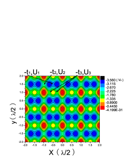
Figure 1: (color online) Geometry of the double-well lattice. It is generated by superposition of laser standing waves along $x$- and $y$-axis: $V(x,y)\!=\!-\!V_{0}{\rm sin}^{2}(k_{1}x)\!-\!V_{0}{\rm sin}^{2}(k_{2}x)\!-\!2V_{0}{\rm sin}^{2}(k_{3}y)$, where $2k_{1}\!\!\!=\!\!k_{2}\!\!\!=\!\!2k_{3}\!\!\!=\!\!2\pi/\lambda$ and $\lambda$ is the laser wavelength. $t_{\sigma}$ are tunnelling amplitudes, and $U_{\sigma}$ ($\sigma\!=\!1,2,3$) are intra- ($\sigma\!=\!1$) and inter-double-well ($\sigma\!=\!2,3$) interactions.

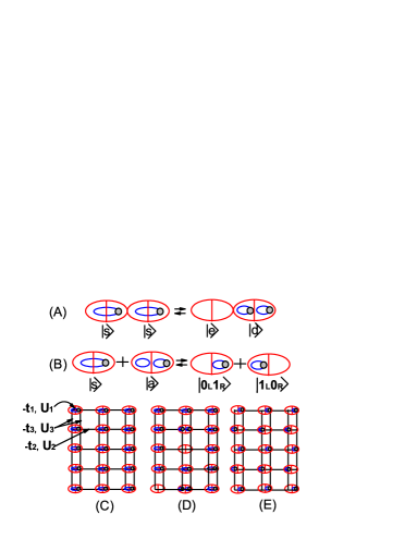
Figure 2: (color online) Bosonic atoms in the double-well lattice with filling factor one. (A) Simultaneous generation of a doubly occupied ($|d\rangle$) and empty ($|e\rangle$) state from the ground state. (B) and (E): Mixing between the symmetric ($|s\rangle$) and anti-symmetric ($|a\rangle$) state results in two degenerate bases $|0_{\rm L}1_{\rm R}\rangle$ and $|1_{\rm L}0_{\rm R}\rangle$. (C) Ground state composed of symmetric state ($|s\rangle$). (D) The double-well lattice in state that mixes $|d\rangle$, $|e\rangle$ and $|s\rangle$ . (E) The checkboard-like insulator state characterized by wave vectors $(\pi,0)$ or $(0,\pi)$.

Particle tunnelling between two sides of a double well makes the single mode approximation unreasonable. At least two modes per site (double well) are required to construct an appropriate low-energy effective Hamiltonian for particles in the double-well lattice. In the specific case with filling factor $\rho=1$ (one atom per double well), and vanishing coupling between different double wells, the ground state $\prod_{k}|s_{k}\rangle$ can be constructed from sDW bases $|s_{k}\rangle$, with $k$ the site (double well) index, since the sDW level is lower than and separated from the other three levels by finite gaps as shown in Fig. 2(C). When tunnelling $t_{2,3}$ between adjacent double wells are strong enough to excite pairs of particles $d$ and $e$ from the ground state $\prod_{k}|s_{k}\rangle$, mobility via $d$ and $e$ appears and the system are eventually in a fluid phase. The eigen wavefunction can now be build up from double-well bases that mainly mix the three primary bases $|s\rangle$, $|d\rangle$, $|e\rangle$ as $[\cos\theta s_{k}^{{\dagger}}+\sin\theta(d_{k}^{{\dagger}}+e^{i\eta}e_{k}^{{\dagger}}]|\phi\rangle$. In this mixed state, pseudo particles $e$ and $d$ play a role similar to what the hole and electron do in electronic crystal materials as schematically shown in Fig. 2(A) and (D). On the other hand, repulsive interactions between atoms trapped in adjacent double wells favour insulator state with characterization wave vectors indicated by $(\pi,0)$ or $(0,\pi)$ as shown in Fig. 2(E). If the filling factor $\rho$ changes from zero (empty) to $2$ (two atoms per double well), there will appear other exotic commensurate and incommensurate insulator phases such as $1/4$ or $1/8$ depleted insulator phases.

When the filling factor is about one, the symmetric basis $|s\rangle$ is a good starting point to construct an variational wave function at low temperatures. Applying the mean-field approximation $\langle s^{\dagger}\rangle=\langle s\rangle=\bar{s}$ to the model Hamiltonian (12), and neglecting the site dependence of chemical potentials $\mu_{r}$ by writing $\mu_{r}=\mu$, i.e., the external confining potential and other kinds of well depth fluctuations are not considered here, the effective Hamiltonian can be written as

$$H_{\rm eff}(\bar{s},\mu,\nu) = H_{\rm DW}(s^{\dagger},s\!\!\rightarrow\!\!\bar{s};\mu_{r}\!\!\rightarrow\!\!\mu)\!+\!2N\mu\rho$$

$$\!\!-\nu\sum_{r}(a^{\dagger}_{r}a_{r}\!+\!e^{\dagger}_{r}e_{r}\!+\!\bar{s}^{2}\!+\!d^{\dagger}_{r}d_{r}\!-\!1),$$

where the Lagrangian multiplier $\nu$ is introduced to assures the constraint condition in Eqn. (7) under the mean field approximation. If only bilinear terms of pseudo particles $d$, $e$ and $a$ are retained, the effective Hamiltonian is readily diagonalized by Fourier-Bogliubov transformations as

$$H=\sum_{k,\alpha}\omega^{\alpha}_{k}(\alpha^{\dagger}_{k}\alpha_{k}+\frac{1}{2})+E_{0},$$ (13)

where $\alpha=\tilde{d},\tilde{e},\tilde{a}$ and

$$E_{0} = -\frac{1}{4}\lambda\bar{s}^{4}(t_{2}+2t_{3})+\bar{s}^{2}[-t_{1}+\frac{1}{2}\lambda(t_{2}+2t_{3})-\mu-\nu]$$

$$+\mu(\frac{3}{2}+\rho)+\frac{5}{2}\nu+\frac{1}{2}(\lambda-1)t_{1},$$

and

$$\omega^{\tilde{d},\tilde{e}}_{k} = \sqrt{A^{2}_{k}-\bar{s}^{4}\eta^{2}_{k}}\pm B_{k},$$

$$\omega^{\tilde{a}}_{k} = \sqrt{C^{2}_{k}-\bar{s}^{4}\xi^{2}_{k}},$$

with

$$A_{k} = -\frac{\lambda}{2}t_{1}-\mu-\nu+\bar{s}^{2}\eta_{k},$$

$$B_{k} = -\frac{\lambda}{2}t_{1}-\mu,$$

$$C_{k} = t_{1}-\mu-\nu-\lambda\bar{s}^{2}(t_{2}+\!2t_{3})+\bar{s}^{2}\xi_{k},$$

$$\eta_{k} = -t_{2}(\lambda+{\rm cos}{k_{x}})-2t_{3}({\rm cos}{k_{y}}+\lambda),$$

$$\xi_{k} = \lambda(t_{2}{\rm cos}{k_{x}}-2t_{3}{\rm cos}{k_{y}}).$$

III.2 Hard-core Statistics

In contrast to identical bosons that obey the ordinary commutation relation, hard-core atoms follow the hard-core bosonic statistics. Hard-core bosonic statistics has been demonstrated to be a powerful tool in studying thermodynamic properties of triplon excitations in spin-dimer systems troyer ; ruegg05 . Similarly, we apply the hard-core statistics to hard-core bosonic atoms in the double-well optical lattice. Consider the state subspace $S_{N}^{M}$ that has $M$ pseudo-particle excitation ($\tilde{e}$,$\tilde{d}$,$\tilde{a}$ in the present paper) over the ground state ($\prod_{k}|s_{k}\rangle$) in a $N$-sites lattice. If such excitations are regarded as identical bosons, dimensions of $S_{N}^{M}$ read as

$$g_{\rm IB}(N,M)=\left(\begin{array}[]{c}3N+M-1\\ M\end{array}\right).$$ (16)

However, the real dimensions of $S_{N}^{M}$ should be

$$g(N,M)=\left(\begin{array}[]{c}N\\ M\end{array}\right)\times 3^{M}.$$ (19)

In the case when $N\gg M\gg 1$, the ratio

$$\frac{g(N,M)}{g_{\rm IB}(N,M)}\approx\exp\left[-\left(\frac{2M}{\sqrt{3N}}\right)^{2}\right].$$

When the typical energy of thermal fluctuations is much less than the least excitation gap, the number of pseudo particles $M\ll\sqrt{N}$, and the real dimensions of $S_{N}^{M}$ are approximately equal to that of identical bosons. The equilibrium properties at finite temperatures can be discussed based on identical bosons. At higher temperatures, when $M\gtrsim\sqrt{N}$, the identical bosons is not suitable to describe the equilibrium properties of such systems.

Applying Troyer et al.’s method troyer to double-well lattices, the distribution of pseudo particles can be derived from partition function of distinguishable bosonic particles in $S_{N}^{M}$. The partition function reads as

$$Z_{\rm B}(N,M)=\sum_{k,\alpha}e^{-\beta\omega^{\alpha}_{k}},$$

where $\alpha$ sums over $\tilde{d},\tilde{e},\tilde{a}$ and $\beta=1/k_{B}T$ with $k_{B}$ the Boltzmann constant. The partition function $Z(N)$ of hard-core pseudo-particles can be obtained by rescaling the dimensions of subspace $S_{N}^{M}$ as

$$Z(N) = \sum_{M=0}^{N}\frac{g(N,M)}{(3N)^{M}}Z_{\rm B}(N,M)$$

$$= \left[1+\sum_{\alpha}\frac{1}{N}\sum_{k}e^{-\beta\omega^{\alpha}_{k}}\right]^{N}.$$

The number of hard-core pseudo-particles per site can be written as

$$n^{\alpha}_{k}=e^{-\beta\omega^{\alpha}_{k}}\Bigg{/}\Big{[}1+\frac{1}{N}\sum_{k,\alpha}e^{-\beta\omega^{\alpha}_{k}}\Big{]}.$$ (20)

where $\alpha$ sums over $\tilde{d}$, $\tilde{e}$, and $\tilde{a}$.

III.3 Self-consistent Saddle-point Equations

Calculations of the partition function for Hamiltonian (13) give the free energy per double well as

$$f=E_{0}/N-\frac{1}{N}\sum_{k,\alpha}\beta{\rm ln}\left[\frac{1}{2}{\rm csch}\left(\frac{\beta\omega^{\alpha}_{k}}{2}\right)\right].$$ (21)

The saddle-point equations of $f$ with respect to $\bar{s}^{2}$, $\mu$, and $\nu$ can be self-consistently solved. The self-consistent equations are written as

$$-\!\frac{1}{2}\lambda(\bar{s}^{2}\!-\!1)(t_{2}\!+\!2t_{3})\!-\!\mu-\!\nu\!-\!t_{1}\!+\!\frac{1}{N}\sum_{k}\Big{[}(n^{\alpha}_{k}\!+\!n^{\beta}_{k}\!+\!1)\frac{A_{k}\eta_{k}\!-\!\bar{s}^{2}\eta^{2}_{k}}{\sqrt{A^{2}_{k}\!-\!\bar{s}^{4}\eta^{2}_{k}}}\!+\!(n^{\gamma}_{k}\!+\!\frac{1}{2})\frac{-\!\lambda C_{k}(t_{2}\!+\!t_{2})\!+\!C_{k}\xi_{k}\!-\!\bar{s}^{2}\xi^{2}_{k}}{\sqrt{C^{2}_{k}\!-\!\bar{s}^{4}\xi^{2}_{k}}}\Big{]}\!=\!0,$$

$$\frac{5}{2}\!-\!\bar{s}^{2}\!-\!\frac{1}{N}\sum_{k}\Big{[}(n^{\alpha}_{k}\!+\!n^{\beta}_{k}\!+\!1)\frac{A_{k}}{\sqrt{A^{2}_{k}\!-\!\bar{s}^{4}\eta^{2}_{k}}}\!+\!(n^{\gamma}_{k}\!+\!\frac{1}{2})\frac{C_{k}}{\sqrt{C^{2}_{k}\!-\!\bar{s}^{4}\xi^{2}_{k}}}\Big{]}\!=\!0,$$

$$-1\!+\!\rho\!+\!\frac{1}{N}\sum_{k}(n^{\beta}_{k}\!-\!n^{\alpha}_{k})\!=\!0.$$ (22)

IV Excitation Spectra and Thermodynamics

IV.1 Excitation Spectra

Figs. 3-5 show the excitation spectra at vanishing temperatures of hard-core bosonic system in the double-well lattice with $\lambda=-0.4$, $t_{2}/t_{1}=t_{3}/t_{1}=0.1$, and $\rho=1$. It can be seen from theses figures that $\tilde{a}$ level is higher than $\tilde{d}$ level and $\tilde{d}$ level is higher than $\tilde{e}$ level. Hence, the lowest excitation seems to be $\omega_{k}^{\tilde{e}}$. However, under the condition of hard-core limit and filling factor one, the excitation processes can be expressed as $\bar{s}+\bar{s}\rightarrow\tilde{d}+\tilde{e}$, since the pseudo particles $\tilde{e}$ and $\tilde{d}$ are simultaneously excited. Therefore, the lowest energy needed to create excitations over the ground state is not the gap of $\tilde{e}$ but the total energy required to generate $\tilde{d}$ and $\tilde{e}$ pseudo particle pairs. The average energy per particle reads as $(\omega_{k}^{\tilde{e}}+\omega_{k}^{\tilde{d}})/2=\sqrt{A^{2}_{k}-\bar{s}^{4}\eta^{2}_{k}}$.

The $\lambda$ dependence of excitation gaps $\Delta_{\alpha}$, middle values $M_{\alpha}$, and half band widths $HW_{\alpha}$ is shown in Fig. 6 and Fig. 7. Considering the degeneracy between $\omega^{\tilde{d}}_{k}$ and $\omega^{\tilde{e}}_{k}$, the relationship $\mu=-\frac{1}{2}\lambda t_{1}$ is satisfied. The gaps, middle values of the excitation spectra $\omega^{\tilde{d}}_{k}$ and $\omega^{\tilde{e}}_{k}$ are formulated by

$$\Delta_{\tilde{d},\tilde{e}} = \sqrt{|\nu|[|\nu|-2\bar{s}^{2}(\lambda+1)(t_{2}+2t_{3})]}~{}~{}(k_{x}=k_{y}=0),$$

$$M_{\tilde{d},\tilde{e}} = \sqrt{|\nu|[|\nu|-2\bar{s}^{2}\lambda(t_{2}+2t_{3})]}.$$

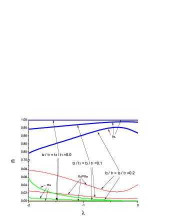
Figure 9: (color online) Inter-particle interaction dependence of empty($n_{e}$), singly ($n_{a}$, $n_{s}$) and doubly ($n_{d}$) occupied double-well numbers at tunnellings $t_{2}/t1=t_{3}/t_{1}=0.0,0.1,0.2$, temperature $T/t_{1}=0.1$, and filling factor $\rho=1$.

As can be seen in Fig. 6, with $|\lambda|$ increasing from $0.5$, $M_{\tilde{d},\tilde{e}}$ is lifted while $HW_{\tilde{d},\tilde{e}}$ is narrowed. This is why the gap is lifted and the occupation number turns bigger (in contrast to $e^{-\beta\omega^{\tilde{d},\tilde{e}}}$) (Fig. 9) with increasing repulsions at fixed temperature.

While strengthening the repulsive potential ($\lambda<0$), the gap $\Delta_{\tilde{a}}$ of the antisymmetric singly occupied level decreases to zero, since the repulsions between nearest double wells keep the atoms away from each other. Consequently, the ground state of a two-fold degenerate checkboard-like insulator, which mixes the symmetric and anti-symmetric state $\prod_{r}({\rm cos}\theta s^{\dagger}_{r}+{\rm sin}\theta a^{\dagger}_{r})|\phi\rangle$ with $\theta\rightarrow\pm\pi/4$, can be expected.

To explore the effect of $\nu$ on the excitation spectra, $\lambda$ dependence of gaps with $t_{2}=t_{3}=0.0,0.1,0.2$ is depicted in Fig. 7. When $t_{2}=t_{3}=0$, the system is made up of isolated double wells and the eigen energy level of the antisymmetric state does not depends on $\lambda$, as defined in Eqn. (6) and shown in Fig. 7. Comparing with the the diagonalized excitation spectra $\omega^{\tilde{a}}_{k}$ in Eqn. (13), the relationship $|\nu|=(1-\frac{\lambda}{2})t_{1}$ can be reached. Substituting this expression into $\omega^{\tilde{d}}_{k}$ and $\omega^{\tilde{e}}_{k}$ , we reobtain the linear relation $\Delta_{\tilde{d},\tilde{e}}=M_{\tilde{d},\tilde{e}}=|\nu|=(1-\frac{\lambda}{2})t_{1}$.

Figure 3: (color online) The excitation spectra of pseudo particles $\tilde{d}$ at $\lambda=-0.4$, $t_{2}/t_{1}=t_{3}/t_{1}=0.1$, and $\rho=1$.

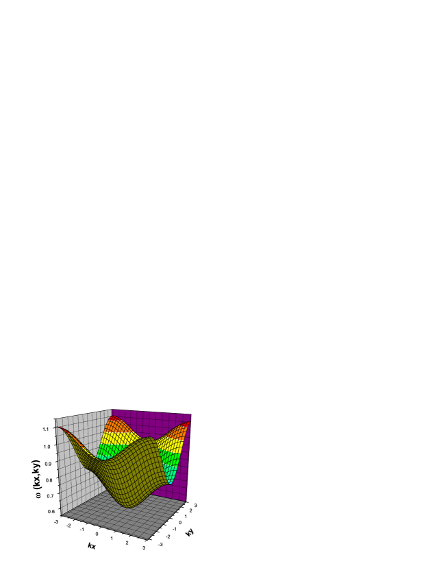
Figure 4: (color online) The excitation spectra of pseudo particles $\tilde{e}$ at $\lambda=-0.4$, $t_{2}/t_{1}=t_{3}/t_{1}=0.1$, and $\rho=1$.

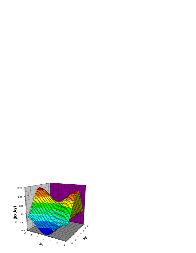
Figure 5: (color online) The excitation spectra of pseudo particles $\tilde{a}$ at $\lambda=-0.4$, with $t_{2}/t_{1}=t_{3}/t_{1}=0.1$, and $\rho=1$.

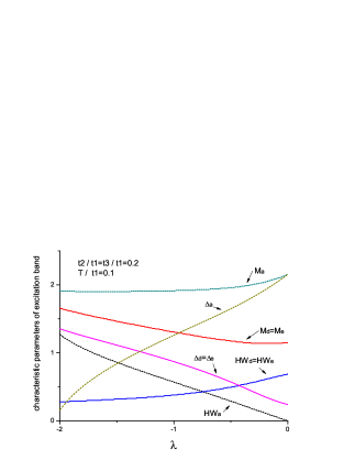
Figure 6: (color online) Curves showing the dependence of gap $\Delta_{\alpha}$, middle values $M_{\alpha}$, and half band widths $HW_{\alpha}$ of excitation spectra on the nearest-neighbour repulsive interactions with $t_{2}/t_{1}=t_{3}/t_{1}=0.2$, $T/t_{1}=0.1$ and $\rho=1$.

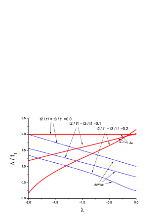
Figure 7: (color online) Comparison of dependence of excitation gaps on the nearest-neighbour repulsive interactions with different tunnellings $t_{2}/t_{1}=t_{3}/t_{1}=0.0,0.1,0.2$, at $T/t_{1}=0.1$ and $\rho=1$.

IV.2 Equilibrium Properties at Finite Temperatures

Fig. 8 shows the temperature dependence of the critical tunnellings $t_{2}$ and $t_{3}$, at $\lambda=-0.4$ and $\rho=1$. The critical values are determined by setting the lowest excitation energy gap zero. In the region under the critical line shown in Fig. 8, the ground sate wave function is modified from $\Psi_{1}=\prod_{i=1}^{N}|s\rangle$ to $\Psi^{\prime}_{1}=[\sum_{r}(1-\tilde{d}_{r}^{{\dagger}}-\tilde{e}_{r}^{{\dagger}}-\tilde{a}_{r}^{{\dagger}})]^{N}|\phi\rangle$.

The critical tunnelling amplitude increases with temperature, which can be explained as follows. Thermal fluctuations lead to finite occupations in excited levels $|\tilde{d}\rangle$ and $|\tilde{{e}}\rangle$ (Fig. 10), and therefore suppress the influence of quantum tunnelling so that a larger tunnelling amplitude is required to collapse the excitation gap as is discussed at the end of Section II. It is noted that the number of pseudo particle $\tilde{d}$ is the same to that of $\tilde{e}$, suggesting that these two types of pseudo particles are simultaneously created through the scattering process $\bar{s}+\bar{s}\rightarrow\tilde{d}+\tilde{e}$. Even near vanishing temperatures at which gapped excitations are few, a finite number of doubly occupied and empty double wells still survive. That is due to the overlap between Wannier wave functions of nearest double wells characterized by tunnellings $t_{\sigma}$ $(\sigma=2,3)$ and the inter-atom interactions $-\lambda t_{\sigma}$. When temperature is high enough, the occupation number per Wannier level asymptotically equals $1/4$ as shown in Fig. 10, which verifies the necessity of the hard-core statistics.

Fig. 11 shows the temperature dependence of heat capacity. It is easy to see that a wide peak appears at temperature near $0.5t_{1}$. In the range of $T>0.5t_{1}$, the heat capacity slowly decreases with temperature. This reflects the hard-core nature of bosonic atoms studied in this work. While decreasing temperature from $0.5t_{1}$ to $0.125t_{1}$, the capacity decreases rapidly since the excitations gaps are finite at the given parameters. When $T<0.125t_{1}$, the capacity is negligibly small because all double wells are in $|s\rangle$ state except contributions from few pseudo-particles $\tilde{d}$ and $\tilde{e}$. Although experimental results about the equilibrium properties mentioned above are not available yet, there are quite a few experimental and theoretical works on the thermodynamic properties of bosonic atoms in ordinary optical lattices garcia ; gerbier . In such systems, the influence of finite temperatures on the phase diagram was emphasized by comparing numerical simulations with experimental results mahmud . It can be expected that the effects of finite temperatures on the properties of atomic gases in optical lattice will attract more attentions.

Figure 8: Temperature (T) dependence of the critical tunnellings between nearest double wells, $t_{2}$ and $t_{3}$, which collapse the lowest excitation gaps at $\lambda=-0.4$ and $\rho=1$.

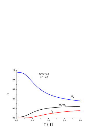
Figure 10: (color online) Temperature dependence of empty($n_{e}$), singly ($n_{a}$, $n_{s}$) and doubly ($n_{d}$) occupied double-well numbers at tunnellings $t_{2}/t_{1}=t_{3}/t_{1}=0.2$, $\lambda=-0.4$, and filling factor $\rho=1$.

Figure 11: Temperature dependence of heat capacity of hard-core bosonic atoms in the double-well lattice at tunnellings $t_{2}/t_{1}=t_{3}/t_{1}=0.1$, $\lambda=-0.4$, and filling factor $\rho=1$.

IV.3 Filling Factors Unequal to One

To study excitation spectra and thermodynamic properties of other phases appearing at filling factors unequal to one, it is necessary to mix the bases defined in section II. SU(4) rotation transformations can be employed to accomplish such mixing, the same as what is done in spin-dimer systems becker2001 ; vojta2013 ; penc2011 . The ground sate $\tilde{\Psi}$ can be obtained by minimizing the system energy $\langle\tilde{\Psi}|H|\tilde{\Psi}\rangle$, where $\tilde{\Psi}$ is the system wavefunction that is made up of double-well mixing bases determined by matrix elements of SU(4) transformations. When the transformation matrix for the lowest double-well basis is determined, the rest double-well bases corresponding to excited levels can also be obtained, as they are determined by the same set of variational parameters. Based on the mixing bases constructed, other phases beyond the fluid and checkbaord-like insulator phases studied in this work could be systematically investigated, too. As has been stressed becker2001 , the orthogonality of mixed bases must be guaranteed in order to correctly describe other ordered phases, such as $1/4$ or $1/8$ depleted commensurate or incommensurate insulator phases. Such generalized cases are quite interesting and will be regarded as our next work.

V Conclusions

In summary, a generalized coupled representation for bosonic atoms in double-well lattices has been obtained by exploiting the mapping relationship between atomic occupation state and coupled bases for spin-dimer systems. Then the coupled representation is applied to the hard-core case with filling factor one. The excitation spectra and thermodynamic properties of such systems are investigated. Starting with a variational ground state wavefunction made of singly occupied symmetric double-well bases, the excitation processes are described by creating pseudo-particles pairs $\tilde{d}$ and $\tilde{e}$, and pseudo-particles $\tilde{a}$. $\tilde{d}$, $\tilde{e}$ and $\tilde{a}$ correspond to doubly occupied and empty double wells and antisymmetric singly occupied double wells, respectively. It is demonstrated that hard-core statistics is required to precisely describe the equilibrium properties of bosonic atoms in double-well lattices at finite temperatures. The critical tunnelling amplitudes increase monotonically with temperature. This behaviour is qualitatively explained based on the effects of thermodynamic fluctuations on the quantum tunnelling. The heat capacity and particle numbers based on the hard-core statics are also calculated which need future experimental verifications.

References

- (1) M. Greiner, O. Mandel, T. Esslinger, T.W. Hänsch and I. Bloch, Nature 415, 39 (2002).
- (2) M. Lewenstein, A. Sanpera, V. Ahufinger, B. Damski, A. Sen and U. Sen, Adv. Phys. 56, 243 (2007).
- (3) I. Bloch, J. Dalibard and W. Zwerger, Rev. Mod. Phys. 80, 885 (2008).
- (4) V. I. Yukalov, Laser Phys. 19, 1 (2009).
- (5) L. Santos, M. A. Baranov, J. I. Cirac, H.-U. Everts, H. Fehrmann, and M. Lewenstein, Phys. Rev. Lett. 93, 030601 (2004).
- (6) S. Fölling, S. Trotzky, P. Cheinet, M. Feld, R. Saers, A. Widera, T. Müller, and I. Bloch, Nature 448, 1029 (2007).
- (7) J. Sebby-Strabley, M. Anderlini, P. S. Jessen and J. V. Porto, Phys. Rev. A 73, 033605 (2006).
- (8) I. Danshita, J. E. Williams, C. A. R. Sá de Melo, and C. W. Clark, Phys. Rev. A 76, 043606 (2007).
- (9) P.-B. He, Q. Sun, P. Li, S.-Q. Shen, and W. M. Liu, Phys. Rev. A 76, 043618 (2007).
- (10) S.-J. Jiang, X.-L. Yu, and W. M. Liu, Phys. Rev. A 84, 063608 (2011).
- (11) V. M. Stojanovi, C. Wu, W. V. Liu, and S. Das Sarma, Phys. Rev. Lett. 101, 125301 (2008).
- (12) V. I. Yukalov and E. P. Yukalova, Phys. Rev. A 78, 063610 (2008).
- (13) D. S. Petrov, and G. V. Shlyapnikov, Phys. Rev. A. 64, 012706 (2001).
- (14) M. Wouters, J. Tempere, and J. T. Devreese, Phys. Rev. A. 68, 053603 (2003).
- (15) L. M. Duan, E. Demler and M. D. Lukin, Phys. Rev. Lett. 91, 090402 (2003).
- (16) S. Trotzky, P. Cheinet, S. Fölling, M. Feld, U. Schnorrberger, A. M. Rey, A. Polkovnikov, E.A. Delmer, M.D. Lukin and I. Bloch, Science 319, 295 (2008).
- (17) Y. A. Chen, S. Nascimb´ene, M. Aidelsburger, M. Atala, S. Trotzky, and I. Bloch, Phys. Rev. Lett. 107, 210405 (2011).
- (18) J. Sebby-Strabley, B. L. Brown, M. Anderlini, P. J. Lee, W. D. Phillips, J. V. Porto and P. R. Johnson, Phys. Rev. Lett. 98, 200405 (2007).
- (19) M. Anderlini, P. J. Lee, B. L. Brown, J. Sebby-Strabley, W. D. Phillips and J. V. Porto, Nature 448, 452 (2007).
- (20) I. Bloch, Nature 453, 1016 (2008).
- (21) S. Sachdev and R. N. Bhatt, Phys. Rev. B 41, 9323 (1990).
- (22) B. Kumar, Phys. Rev. B 82, 054404 (2011).
- (23) T. Nikuni, M. Oshikawa, and H. Tanaka, Phys. Rev. Lett. 84, 5868 (2000).
- (24) Ch. Rüegg, N. Cavadin, A. Furrer, H. Güdel, K. Krämer, H. Mutka, A. Wildes, K. Habicht, and P. Vorderwisch, Nature 423, 62 (2003).
- (25) B. Xu, H. Wang and Y. Wang, Phys. Rev. B 77, 014401(2008).
- (26) T. Matsubara and H. Matsuda, Prog. Theor. Phys. 16, 569 (1956).
- (27) T. Giamarchi, C. Rüegg, and O. Tchernyshyov, Nature Phys. 4, 198 (2008).
- (28) J. C. Hubbard, Proc. Roy. Soc. A 276, 238 (1963).
- (29) V. M. Stojanovi, C. Wu, W. V. Liu, and S. Das Sarma, Phys. Rev. Lett. 101, 125301 (2008).
- (30) M. D. Girardeau, J. Math. Phys. (N.Y.) 1, 516 (1960).
- (31) D. Jaksch, C. Bruder, J. I. Cirac, C. W. Gardiner, and P. Zoller, Phys. Rev. Lett. 81, 3108 (1998).
- (32) V. W. Scarola, and S. Das Sarma, Phys. Rev. Lett. 95, 033003 (2005).
- (33) M. Troyer, H. Tsunetsugu and D. Würtz, Phys. Rev. B 50, 13515 (1994).
- (34) Ch. Rüegg, B. Normand, M. Matsumoto, Ch. Niedermayer, A. Furrer, K. W. Krämer, H.-U. Güdel, Ph. Bourges, Y. Sidis and H. Mutka, Phys. Rev. Lett. 95, 267201 (2005).
- (35) K. Jimenez-Garcia, R. L. Compton, Y.-J. Lin, W. D. Phillips, J. V. Porto, and I. B. Spielman, Phys. Rev. Lett. 105, 110401 (2010).
- (36) F. Gerbier, Phys. Rev. Lett. 99, 120405 (2007).
- (37) K. W. Mahmud, E. N. Duchon, Y. Kato, N. Kawashima, R. T. Scalettar, N. Trivedi, Phys. Rev. B 84, 054302 (2011).
- (38) T. Sommer, M. Vojta, and K.W. Becker, Eur. Phys. J. B 23,329 (2001).
- (39) M. Vojta, Phys. Rev. Lett. 111, 097202 (2013).
- (40) J. Romhányi, K. Totsuka, and K. Penc, Phys. Rev. B 83, 024413 (2011).