Metastability of Morse–Smale dynamical systems
perturbed by heavy-tailed Lévy type noise

Abstract

We consider a general class of finite dimensional deterministic dynamical systems with finitely many local attractors $K^{\iota}$ each of which supports a unique ergodic probability measure $P^{\iota}$, which includes in particular the class of Morse–Smale systems in any finite dimension. The dynamical system is perturbed by a multiplicative non-Gaussian heavy-tailed Lévy type noise of small intensity $\varepsilon>0$. Specifically we consider perturbations leading to a Itô, Stratonovich and canonical (Marcus) stochastic differential equation. The respective asymptotic first exit time and location problem from each of the domains of attractions $D^{\iota}$ in case of inward pointing vector fields in the limit of $\varepsilon\searrow 0$ was solved by the authors in [21]. We extend these results to domains with characteristic boundaries and show that the perturbed system exhibits a metastable behavior in the sense that there exits a unique $\varepsilon$-dependent time scale on which the random system converges to a continuous time Markov chain switching between the invariant measures $P^{\iota}$. As examples we consider $\alpha$-stable perturbations of the Duffing equation and a chemical system exhibiting a birhythmic behavior.

Keywords: hyperbolic dynamical system; Morse-Smale property; stable limit cycle; small noise asymptotic; $\alpha$-stable Lévy process; multiplicative noise; stochastic Itô integral; stochastic Stratonovich integral; stochastic canonical (Marcus) differential equation; multiscale dynamics; metastability; embedded Markov chain; randomly forced Duffing equation; birhythmic behavior.

2010 Mathematical Subject Classification: 60H10; 60G51; 37A20; 60J60; 60J75; 60G52.

1 Introduction

Consider a multivariate deterministic dissipative dynamical system given as the solution flow of a finite-dimensional ordinary differential equation $\dot{u}=f(u)$. We assume that it has finitely many local attractors $K^{\iota}$, each of which is contained in a domain of attraction $D^{\iota}$. By definition, for each initial condition in $D^{\iota}$ the trajectory never leaves $D^{\iota}$ and converges to $K^{\iota}$. We shall not impose specific conditions on the geometry of the attractors instead we assume that the time averages of the trajectories converge weakly to the unique invariant probability measure $P^{\iota}$ supported on $K^{\iota}$ as time tends to infinity. This convergence should be uniform w.r.t. the trajectory’s initial condition over compact subsets of the domain $D^{\iota}$. Dynamical systems with finitely many stable fixed points $K^{\iota}=\{\mathfrak{s}^{\iota}\}$ or stable limit cycles belong to the evident examples of systems under consideration.

The behavior of the system changes significantly in the presence of a perturbation by noise, however small its intensity $\varepsilon>0$ may be. In the generic situation, the perturbed solution relaxes from the initial position and remains — usually for a very long time — close to the attractor $K^{\iota}$ of the initial domain $D^{\iota}$. However with probability one, it exits from $D^{\iota}$ at some random time instant in an abrupt move and immediately enters another domain $D^{j}$, $j\neq\iota$, where the same performance starts anew. In this way, step by step and after possibly many repetitions the process visits all domains, not all of them of course with the same frequency and for an equally long period. In the literature, such a behavior of the trajectory is referred to as metastability.

In Galves et al. [17, p. 1288], the authors describe the metastable behavior of a deterministic dissipative dynamical system subject to small Gaussian perturbations as follows: “A stochastic process with a unique stationary invariant measure, which […] behaves for a very long time as if it were described by another “stationary” measure (metastable state), performing […] an abrupt transition to the correct equilibrium. In order to detect this behavior, it is suggested […] to look at the time averages along typical trajectories; we should see: apparent stability — sharp transition — stability.”

In any case, the transition times between different domains of attraction tends to infinity as the noise amplitude $\varepsilon$ goes to zero, however, the growth rate of the expected transition time as well as the probability to pass from $D^{\iota}$ to $D^{j}$ strongly depend on the nature of the noise and the properties of the underlying deterministic system.

In this article, we study the behavior of a dynamical system given as the solution flow of a rather generic finite-dimensional ordinary differential equation $\dot{u}=f(u)$ subject to a small noise perturbation by a multiplicative Lévy type noise with a discontinuous, non-Gaussian heavy-tailed component. Since its dynamics will differ strongly from the case of Gaussian perturbations, let us briefly discuss the underlying deterministic dynamical system and summarize the metastability results in the Gaussian case.

1.1 Generic dynamical systems under consideration

There is a large body of literature on the classification of deterministic dynamical systems and their stability properties, which we obviously cannot review here. Instead, we will restrict ourselves to the minimal necessary orientation of the reader about the systems we consider in this article. In the sequel we will mainly refer to the overview articles [2, 39], introductory books [19, 44], and the extensive list of references therein.

The class of dynamical systems we consider has finitely many well separated local attractors, with respective domains of attractions. We suppose that all trajectories starting in a compact set inside the a domain of attraction converge weakly and uniformly to a unique invariant probability measure concentrated on the local attractor. This invariant measure is assumed to be parametrized by the sojourn times of the dynamical system on the attractor. Since this class is not classical we briefly give a subsumption of its relation into well-known classes.

The simplest class of examples are gradient systems, where $f$ is given as the gradient $-\nabla U$ of a smooth non-degenerate multi-well potential function $U\colon\mathbb{R}^{d}\rightarrow\mathbb{R}$ with finitely many minima $\mathfrak{s^{\iota}}$, $\iota=1,\dots,\kappa$. In this case, the local invariant measure is given as a unit point mass $P^{\iota}=\delta_{\mathfrak{s}^{\iota}}$.

A finite-dimensional dynamical system is said to have the Morse–Smale property if the set of its non-wandering points consists of a union of finitely many periodic orbits (limit cycles), whose points are all hyperbolic and whose invariant manifolds meet transversally. For each of the non-trivial periodic stable orbits of the non-wandering sets of the Morse–Smale system, which parametrizes the corresponding limit cycle, say, $K^{\iota}$, we can define the invariant measure $P^{\iota}$ by

$$P^{\iota}(A):=\frac{1}{\mathcal{T}_{\iota}}\int_{0}^{\mathcal{T}_{\iota}}\mathbf{1}_{A}(u(s;x))\,ds,\quad A\mbox{ Borel },\quad u(0;x)=x\in K^{\iota},\ u(t+\mathcal{T}_{\iota};x)=u(t;x).$$

In the Appendix it is shown that a Morse–Smale dynamical system in any dimension over a compact domain satisfies the required property that for all initial conditions uniformly bounded from the separating manifold, the time average of the trajectory converges weakly to $P^{\iota}$. In dimensions $1$ and $2$ Morse–Smale systems coincide with the class of structurally stable systems which are generic in the sense of being an open dense subset of all dynamical systems generated by $\mathcal{C}^{2}$ vector fields, see [37, 40]. It is known for a long time that in higher dimensions $d\geqslant 3$, the Morse–Smale systems are a subclass of structurally stable systems but that the latter fail to be generic.

We emphasize, however, that our assumptions are not restricted to the Morse–Smale systems, since we require only the existence of finitely many local attractors satisfying the above mentioned statistical property on the convergence of the time averages.

Finally we remark, that from a slightly different perspective we can interpret the finitely many invariant measures $P^{\iota}$ as the ergodic components of the so-called Sinai–Bowen–Ruelle measure (SRB-measure, for short), sometimes referred to as the physical measure. For details we refer to the classical text [8] and for a more recent overview to [46].

1.2 The hierarchy of cycles and time scales in the generic Gaussian case

The small noise analysis and metastability results for randomly perturbed dynamical systems of the form $dX_{t}=f(X_{t})dt+\varepsilon\,dW$, $W$ being a Brownian motion (the noise term may be multiplicative as well) may be performed with the help of the large deviations theory by Freidlin and Wentzell [16]. It is well known that with any $D^{\iota}$ that contains a unique point attractor $K^{\iota}=\{\mathfrak{s}^{\iota}\}$ we can associate a positive number $V_{\iota}$ such that the expected exit time from $D^{\iota}$ is asymptotically proportional to $\exp(V_{\iota}/\varepsilon^{2})$ in the limit of $\varepsilon\searrow 0$. This result is a version of what is known as Kramers’ law [30] in the physics and chemistry literature. The constant $V_{\iota}$ can be interpreted as the height of the lowest “mountain pass” on the way from the attractor $\mathfrak{s}^{\iota}$ to the boundary $\partial D^{\iota}$ in the energy landscape given by the so-called quasi-potential determined by the vector field $f$. The same result would hold for an arbitrary attractors $K^{\iota}$ whose points are equivalent w.r.t. the quasi-potential, that is do not require any additional work for transitions between them (for example like in the case of a limit cycle).

Further, for any two domains $D^{i}$ and $D^{j}$, $i\neq j$, there is a number $V_{ij}\geqslant 0$ such that the expected transition time from $D^{i}$ to $D^{j}$ is asymptotically proportional to $\exp(V_{ij}/\varepsilon^{2})$. Note that in the generic case the constants $V_{ij}$ are different and the time scales $\exp(V_{ij}/\varepsilon^{2})$ are thus exponentially separated. This naturally leads to the hierarchy of consecutive transitions of the random trajectory staring in $D^{\iota}$, the so-called the hierarchy of cycles.

Indeed, starting in $D^{\iota}$, we determine the unique sequence of indices $j(0)=\iota$, $j(1),j(2),\dots$, defined such that $V_{j(k-1),j(k)}=\min_{j\neq j(k-1)}V_{j(k-1),j}$, $k\geqslant 0$. The sequence $\{j(k)\}$ is periodic with some period $p_{1}$ and the states $C(1)=\{\iota,j(1),\dots,j(p_{1}-1)\}$ constitute the cycle of the first rank. For $C(1)$ we can analogously define cycles of the higher orders, the last cycle containing all the states $\{1,\dots,\kappa\}$. Each cycle $C$ contains the main state $K(C)$, that is the index of the attractor, in the basin of which the random trajectory spends most of its time before leaving the set $\cup_{j\in C}D^{j}$. For a detailed exposition we refer to Freidlin and Wentzell [16] or to a recent work by Cameron [11].

It is a distinguishing property of a system perturbed by a small Gaussian noise that the hierarchy of cycles, their main states and the logarithmic rates of the associated exponentially large transition times are not random and are determined by the vector field $f$ with the help of the quasipotential.

Various refinements and generalizations of these results include the proof of the convergence of a small noise diffusion $X$ in a double-well potential to a two-state Markov chain [17, 27], a connection between the metastability and the spectrum of the diffusion’s generator [3, 6, 7, 28, 29], or the study of the infinite dimensional systems [4, 9, 10, 14, 15].

1.3 The unique time scale and total communication of states in the generic regularly varying Lévy case

In this paper we treat a $d$-dimensional dynamical system $\dot{u}=f(u)$ perturbed by a (multiplicative) Lévy noise with heavy-tailed jumps, that is a process whose Lévy measure possesses regularly varying tails with the index $-\alpha<0$. As an example of such a perturbation one can have in mind $\alpha$-stable Lévy noise, $\alpha\in(0,2)$.

To our best knowledge, the Markovian systems with heavy-tailed jumps were firstly studied by Godovanchuk [18]. The asymptotics of the first exit times an metastability results in the one-dimensional setting of systems represented by SDEs driven by additive heavy-tailed Lévy processes were obtained in [24, 24]. Further the theory was developed for multivariate systems with heavy-tail multiplicative noise in [26, 36] and for a class of stochastic reaction–diffusion equations in [12].

The behavior of a dynamical system perturbed by heavy jumps differs qualitatively from the Gaussian case. First, the behavior becomes non-local, that is by a single jumps of an arbitrary big magnitude the system may change its state instantly. Second, the power law jumps determining the heavieness of the jumps also determines the unique time scale on which the exits from domains $D^{i}$ and transitions between the domains $D^{i}$ and $D^{j}$ occur.

For simplicitiy let us sketch the case of a small additive perturbation by a stable Lévy process $\varepsilon Z$ with the jump measure $\nu(A)=\int_{A}\|z\|^{-d-\alpha}dz$ . Let $K^{i}=\{\mathfrak{s}^{i}\}$ be a stable point. In this situation, the first exit time from the domain $D^{i}$ has the mean value $Q_{i}/\varepsilon^{\alpha}$ with the prefactor $Q_{i}=\int_{\mathbb{R}^{d}\backslash D^{i}}\|z-\mathfrak{s}^{i}\|^{-d-\alpha}dz$. In other words, the prefactor $Q_{i}$ measures the set of all jump increments of the noise, whose result is the exit from the domain $D^{i}$ at a single jump. We refer to [12, 21, 24, 25] for detailed explanations.

To describe transitions between the different domains of attraction we will see that in contrast to the Gaussian hierarchy of cycles, all mean transition times from the domain $D^{i}$ to $D^{j}$ are asymptotically equivalent to $Q_{ij}/\varepsilon^{\alpha}$ in the limit of small $\varepsilon$ for $Q_{ij}=Q_{i}^{-1}\int_{D^{j}}\|z-\mathfrak{s}^{i}\|^{-d-\alpha}dz$. This means that the transition rates are not well separated for small $\varepsilon$. This generic picture in the heavy-tailed framework may be associated with the very degenerate Gaussian case when all logarithmic rates $V_{ij}$ are identical and the transition behavior is determined by the sub-exponential prefactors. For a very precise asymptotics of these prefactors in the Gaussian setting we refer to Kolokoltsov [29, 28] and Bovier et al. [6].

In [21], we generalize the exit time results to underlying deterministic generic dynamical systems with non-point attractors. The stable state $\mathfrak{s}^{i}$ as a geometric object appearing in the formulae for the mean transition times has to be replaced by a statistical quantity given as the ergodic invariant probability measure $P^{i}$ concentrated on the local attractor $K^{i}$ of the respective domain $D^{i}$. More precisely we prove that a transition time between domains $D^{i}$ and $D^{j}$ asymptotically grows as $\widetilde{Q}_{ij}/\varepsilon^{\alpha}$ with

$$\widetilde{Q}_{ij}=\frac{\int_{K^{i}}\int_{D^{j}}\|z-v\|^{-d-\alpha}dzP^{i}(dv)}{\int_{K^{i}}\int_{\mathbb{R}^{d}\backslash D^{i}}\|z-v\|^{-d-\alpha}dzP^{i}(dv)}.$$

The coefficient $\widetilde{Q}_{ij}$ weights the points on the attractor $K^{i}$ with respect to the corresponding ergodic invariant measure $P^{i}$. For details we refer to the introduction of [21].

We see that generically the expected transition time between any two domains of attraction is proportional to $1/\varepsilon^{\alpha}$. Moreover it is shown that the respectively renormalized transition times are asymptotically exponentially distributed. Let us consider the perturbed path $X^{\varepsilon}$ on the time scale $t/\varepsilon^{\alpha}$. On this time scale we would expect that the process $X^{\varepsilon}(\frac{t}{\varepsilon^{\alpha}})$ spends most of the time in the domains of attraction $D^{i}$ exhibiting instantaneous single jump transitions from the vicinity of the attractor $K^{i}$ to the domain $D^{j}$. Thus the first result of this paper will describe a Markov chain $m=(m_{t})_{t\geqslant 0}$ on the index set $\{1,\dots,\kappa\}$, which will specify the domain of attraction $D^{i}$ the process $X^{\varepsilon}_{\cdot/\varepsilon^{\alpha}}$ currently sojourns. Roughly speaking, this allows us to determine the probability for the process $X^{\varepsilon}_{\cdot/\varepsilon^{\alpha}}$ to visit domains $D^{i_{1}},\dots,D^{i_{n}}$ at prescribed deterministic times $0<t_{1}<\cdots<t_{n}$, $n\geqslant 1$.

In the second part, we prove a stronger result. Under the condition that $X^{\varepsilon}_{t/\varepsilon^{\alpha}}\in D^{i}$ for some $i\in\{1,\dots,\kappa\}$, the process $X^{\varepsilon}$ is naturally located in the vicinity of the attractor $K^{i}$. We will determine the location of $X^{\varepsilon}$ at a slightly randomized observation time $(t+\sigma r_{\varepsilon})\varepsilon^{-\alpha}$, $\sigma$ being an independent random variable uniformly distributed on $[-1,1]$ and $r_{\varepsilon}$ being an arbitrary rate characterizing the time measurement error such that $r_{\varepsilon}\to 0$ and $r_{\varepsilon}/\varepsilon^{\alpha}\to\infty$. We show that in the limit $\varepsilon\to 0$, the location $X^{\varepsilon}_{(t+\sigma r_{\varepsilon})\varepsilon^{-\alpha}}$ is distributed on the attractor $K^{i}$ according to the ergodic measure $P^{i}$, whereas the attractor index $i=m_{t}$ is itself distributed with the law of the Markov chain $m$. Essentially this means that within a given vanishing error bound on the time scale $t/\varepsilon^{\alpha}$ only the statistical aggregate of the behavior $X^{\varepsilon}$ can be perceived.

We can make the intuition presented above rigorous for a general class of additive and multiplicative Lévy noises with a regularly varying Lévy measure. In particular, our main result covers perturbations in the sense of Itô and Stratonovich, as well as in the sense of canonical (Marcus) equation, where jumps in general do not occur along straight lines, but follow the flow of the vector field which determines the multiplicative noise.

In the physics and other natural sciences, Gaussian perturbations of dynamical systems with limit cycle attractors have been considered since quite some time, see e.g. Epele et al. [13], Moran and Goldbeter [35], Hill et al. [20], Kurrer and Schulten [32], Liu and Crawford [34], and Saet and Viviani [42]. As an application of our main result we present two examples in detail: the Duffing equation with two point attractors and a planar system from [35] with two stable limit cycles which lie in one another.

2 Object of study and main result

2.1 Deterministic dynamics

We consider a globally Lipschitz continuous vector field $f\in\mathcal{C}^{2}(\mathbb{R}^{d},\mathbb{R}^{d})$. It is well-known that this assumption is sufficient to establish the existence and uniqueness of the dynamical system, given as the solution flow $\varphi$ of the autonomous ordinary differential equation

$$\dot{u}=f(u),\qquad u(0;x)=x\in\mathbb{R}^{d},$$ (1)

where we denote by $\varphi_{t}(x):=u(t;x)$. Note that the dynamical system can be prolonged to arbitrary negative times.

We assume the following properties of $\varphi$.

1. The set of non-wandering points of $\varphi$ contains finitely many local attractors $K^{\iota}$, $\iota=1,\dots,\kappa$, $\kappa\geqslant 1$, with corresponding open domains of attractions $D^{\iota}$. For definitions we refer to [2] and [19].

2. All non-wandering points of $\varphi$ are hyperbolic and the corresponding invariant manifolds meet transversally.

3. For any $R>0$ such that $\bigcup_{\iota}K^{\iota}\subset B_{R}(0)$, there exits a bounded, measurable, connected set $\mathcal{I}_{R}\subset B_{R}(0)$ with smooth boundary, such that $f\big{|}_{\partial\mathcal{I}_{R}}$ is uniformly inward pointing.

4. For each local attractor $K^{\iota}$ there exists a unique probability measure $P^{\iota}$ supported on $K^{\iota}$, $\operatorname{supp}(P^{\iota})=K^{\iota}$, such that such that for all non-negative, measurable and bounded functions $\psi\colon\mathbb{R}^{d}\rightarrow\mathbb{R}$, any $R>0$ defined in 3, and all closed subsets $A$ contained in the interior of $D^{\iota}\cap\mathcal{I}_{R}$ the limit

   $$\lim_{t\rightarrow\infty}\sup_{x\in A}\frac{1}{t}\int_{0}^{t}\psi(\varphi_{s}(x))ds=\int_{K^{\iota}}\psi(v)P^{\iota}(dv)$$ (2)

   holds true.

2.2 The random perturbation

On a filtered probability space $(\Omega,\mathcal{F},(\mathcal{F}_{t})_{t\geqslant 0},\mathbb{P})$, satisfying the usual hypotheses in the sense of Protter [38], we consider a Lévy process $Z=(Z_{t})_{t\geqslant 0}$ with values in $\mathbb{R}^{m}$, $m\geqslant 1$, and the characteristic function

$$\mathbb{E}e^{i\langle u,Z_{1}\rangle}=\exp\Big{(}-\frac{\langle Au,u\rangle}{2}+i\langle b,u\rangle+\int\Big{(}e^{i\langle u,z\rangle}-1-i\langle u,z\rangle\mathbf{1}_{B_{1}(0)}(z)\Big{)}\nu(dz)\Big{)},\ u\in\mathbb{R}^{m},$$

where $A$ is a symmetric nonnegative definite $m\times m$ (covariance) matrix, $b\in\mathbb{R}^{m}$, and $\nu$ a $\sigma$-finite measure on $\mathbb{R}^{m}$ satisfying $\nu(\{0\})=0$ and $\int_{\mathbb{R}^{m}}(1\wedge\|y\|^{2})\nu(dy)<\infty$. The measure $\nu$ is referred to as the Lévy measure of $Z$, and $(A,\nu,b)$ is called the generating triplet of $Z$.

Let us denote by $N(dt,dz)$ the associated Poisson random measure with the intensity measure $dt\otimes\nu(dz)$ and the compensated Poisson random measure $\widetilde{N}(dt,dz)=N(dt,dz)-dt\nu(dz)$. Consequently, by the Lévy–Itô theorem (see e.g. Applebaum [1, Chapter 2]) the Lévy process $Z$ given above has the following a.s. path-wise additive decomposition

$$Z_{t}=A^{\frac{1}{2}}B_{t}+bt+\int_{(0,t]}\int_{0<\|z\|\leqslant 1}z\widetilde{N}(ds,dz)+\int_{(0,t]}\int_{\|z\|>1}zN(ds,dz),\qquad t\geqslant 0,$$ (3)

with $B=(B_{t})_{t\geqslant 0}$ being a standard Brownian motion in $\mathbb{R}^{m}$. Furthermore, the random summands in (3) are independent. For further details on Lévy processes we refer to Applebaum [1] and Sato [43].

The following assumption about the big jumps of $Z$ is crucial for our theory.

(S.1) The Lévy measure $\nu$ of the process $Z$ is regularly varying at $\infty$ with index $-\alpha$, $\alpha>0$. Let $h\colon(0,\infty)\to(0,\infty)$ denote the tail of $\nu$

$$h(r):=\int_{\|y\|\geqslant r}\nu(dy).$$ (4)

We assume that there exist $\alpha>0$ and a non-trivial self-similar Radon measure $\mu$ on $\bar{\mathbb{R}}^{m}\backslash\{0\}$ such that $\mu(\bar{\mathbb{R}}^{m}\backslash\mathbb{R}^{m})=0$ and for any $a>0$ and any Borel set $A$ bounded away from the origin, $0\notin\overline{A}$, with $\mu(\partial A)=0$, the following limit holds true:

$$\mu(aA)=\lim_{r\rightarrow\infty}\frac{\nu(raA)}{h(r)}=\frac{1}{a^{\alpha}}\lim_{r\rightarrow\infty}\frac{\nu(rA)}{h(r)}=\frac{1}{a^{\alpha}}\mu(A).$$ (5)

In particular, following [5] there exists a positive function $\ell$ slowly varying at infinity such that

$$h(r)=\frac{1}{r^{\alpha}\ell(r)}\qquad\mbox{ for all}\quad r>0.$$

The self-similarity property of the limit measure $\mu$ implies that $\mu$ assigns no mass to spheres centered at the origin of $\mathbb{R}^{m}$ and has no atoms. For more information on multivariate heavy tails and regular variation we refer the reader to Hult and Lindskog [22] and Resnick [41]. The following set of assumptions deals with the multiplicative perturbation of the dynamical system $u$ by the Lévy process $Z$.

(S.2) Consider continuous maps $G\in\mathcal{C}(\mathbb{R}^{d}\times\mathbb{R}^{m},\mathbb{R}^{d})$ and $F,H\colon\mathbb{R}^{d}\rightarrow\mathbb{R}^{d}$ and fix the notation

$$a(x,y):=F(x)F(y)^{*}\qquad\mbox{ for }x,y\in\mathbb{R}^{d},$$

where $F(y)^{*}$ is the transposed (row) vector of $F(y)$. We assume that for any $R>0$ there exists $L=L_{R}>0$ such that $f$, $G$, $H$ and $F$ satisfy the following properties.

1. Local Lipschitz conditions: For all $x,y\in\mathcal{I}_{R}$

   $$\|f(x)-f(y)\|^{2}+\|a(x,x)-2a(x,y)+a(y,y)\|+\|H(x)-H(y)\|^{2}\\ +\|F(x)-F(y)\|^{2}+\int_{B_{1}(0)}\|G(x,z)-G(y,z)\|^{2}\nu(dz)\leqslant L^{2}\|x-y\|^{2}.$$

2. Local boundedness: For all $x\in\mathcal{I}_{R}$

   $$\|f(x)\|^{2}+\|a(x,x)\|+\|H(x)\|^{2}+\|F(x)\|^{2}+\int_{B_{1}(0)}\|G(x,z)\|^{2}\nu(dz)\leqslant L^{2}(1+\|x\|^{2}).$$

3. Large jump coefficient: For all $x,y\in\mathcal{I}_{R}$ and $z\in\mathbb{R}^{m}$

   $$\|G(x,z)-G(y,z)\|\leqslant Le^{L(\|z\|\wedge L)}\|x-y\|.$$

4. Local bound for $G$ in small balls: There exists $\delta^{\prime}>0$ such that for $z\in B_{\delta^{\prime}}(0)$

   $$\sup_{x\in B_{\delta^{\prime}}(K^{\iota})}\|G(x,z)\|\leqslant L.$$

Proposition 2.1.

Let the assumptions (S.2.1–3) be fulfilled. Then for any $\varepsilon,\delta\in(0,1)$, $R>0$ and $x\in\mathcal{I}_{R}$ the stochastic differential equation

$$X_{t,x}^{\varepsilon} =x+\int_{0}^{t}f(X^{\varepsilon}_{s,x})\,ds+\varepsilon\int_{0}^{t}H(X^{\varepsilon}_{s,x})b\,ds+\varepsilon\int_{0}^{t}F(X^{\varepsilon}_{s,x})\,d(A^{\frac{1}{2}}B_{s})$$ (6)

$$\qquad+\int_{0}^{t}\int_{\|z\|\leqslant 1}G(X^{\varepsilon}_{s-,x},\varepsilon z)\widetilde{N}(ds,dz)+\int_{0}^{t}\int_{\|z\|>1}G(X^{\varepsilon}_{s-,x},\varepsilon z)N(ds,dz)$$

has a unique strong solution $(X^{\varepsilon}_{t\wedge\mathbb{T},x})_{t\geqslant 0}$ with càdlàg paths in $\mathbb{R}^{d}$ which is a strong Markov process with respect to $(\mathcal{F}_{t})_{t\geqslant 0}$, where

$$\mathbb{T}=\mathbb{T}_{x}^{R}(\varepsilon) :=\inf\{t\geqslant 0\colon X^{\varepsilon}_{t,x}\notin\mathcal{I}_{R}\}.$$

is the first exit time from $\mathcal{I}_{R}$.

A proof can be found for instance in Ikeda and Watanabe [23], Theorem 9.1, or Chapter 6 in Applebaum [1]. The multiplicative perturbations in the sense of Itô, Fisk–Stratonovich or (canonical) Marcus equations could be of special interest for applications. We refer the reader to Applebaum [1], Ikeda Watanabe [23] and Protter [38] for a general theory of stochastic integration in the Itô and Fisk–Stratonovich sense and to Applebaum [1], Kurtz et al. [33] and Kunita [31] for a construction of the canonical Marcus equations. A brief comparison of these equations can be also found in Pavlyukevich [36].

For example, assume that $Z$ is a pure jump Lévy process with $A=0$, $b=0$, and let $\Phi\colon\mathbb{R}^{d}\to\mathbb{R}^{d\times m}$ be a globally Lipschitz continuous function. Taking

$$G(x,z):=x-\Phi(x)z$$

we yields the Itô SDE with the multiplicative noise

$$X_{t} =x+\int_{0}^{t}f(X_{s})dt+\varepsilon\int_{0}^{t}\Phi(X_{s-})dZ_{s},$$ (7)

To obtain a canonical (Marcus) equation with the multiplicative noise

$$X_{t}^{\diamond} =x+\int_{0}^{t}f(X_{s}^{\diamond})dt+\varepsilon\int_{0}^{t}\Phi(X_{s-}^{\diamond})\diamond dZ_{s}.$$ (8)

we denote by $\psi^{z}(x)=y(1;x,z)$ the solution of the nonlinear ordinary differential equation

$$\begin{cases}&\dot{y}(s)=\Phi(y(s))z,\\ &y(0)=x,\quad s\in[0,1].\end{cases}$$ (9)

and set

$$G(x,z):=\psi^{z}(x).$$

If $L$ is the Lipschitz constant of the matrix function $\Phi$ then the Gronwall lemma implies that

$$\|G(x,z)-G(y,z)\|\leqslant Le^{L\|z\|}\|x-y\|\qquad\forall x,y\in D,z\in\mathbb{R}^{m},$$

what justifies the assumption (S.2.3).

2.3 The main result and examples

For $x\in\mathbb{R}^{d}$, $U\in\mathfrak{B}(\mathbb{R}^{d})$ with $x\notin U$ we denote the set of jump increments $z\in\mathbb{R}^{m}$ which send $x$ into $U$ by

$$E^{U}(x) :=\{z\in\mathbb{R}^{m}\colon x+G(x,z)\in U\}.$$ (10)

We define the measure $Q^{\iota}$ on $\mathfrak{B}(\mathbb{R}^{d})$ assigning

$$Q^{\iota}(U) :=\int_{K^{\iota}}\mu(E^{U}(y))\leavevmode\nobreak\ dP^{\iota}(y),$$ (11)

where $P^{\iota}$ is a measure on $K^{\iota}$ defined in (D.1) and $\mu$ is a regularly varying limiting jump measure appearing in (5). For $\varepsilon>0$ denote

$$\lambda_{\varepsilon}^{\iota} :=\int_{K^{\iota}}\nu\Big{(}\frac{E^{(D^{\iota})^{c}}(y)}{\varepsilon}\Big{)}dP^{\iota}(y)\quad\mbox{ and }\quad h_{\varepsilon}:=h\Big{(}\frac{1}{\varepsilon}\Big{)}.$$

Then the equation (5) implies

$$\lim_{\varepsilon\rightarrow 0+}\frac{\lambda_{\varepsilon}^{\iota}}{h_{\varepsilon}}=Q^{\iota}((D^{\iota})^{c}).$$

The main result of this article is the following metastability result.

Theorem 2.2.

Let assumptions (D.1) and (S.1-2) be fulfilled and suppose that for all $\iota=1,\dots,\kappa$,

$$Q^{\iota}\Big{(}\mathbb{R}^{d}\setminus\bigcup_{\ell=1}^{\kappa}D^{\ell}\Big{)}=0.$$ (12)

Then there exists a continuous-time Markov chain $m=(m_{t})_{t\geqslant 0}$ with values in the set $\{1,\dots,\kappa\}$ and a generator matrix

$$\mathcal{Q}=\begin{pmatrix}-Q^{1}\left(\left(D^{1}\right)^{c}\right)&Q^{1}\left(D^{2}\right)&\dots&Q^{1}(D^{\kappa})\\ \vdots&&&\vdots\\ Q^{\kappa}\left(D^{1}\right)&\dots&Q^{\kappa}(D^{\kappa-1})&-Q^{\kappa}\left(\left(D^{\kappa}\right)^{c}\right)\end{pmatrix}.$$ (13)

such that the following statements hold.

1. Let $N\geqslant 1$, $\iota_{0},\dots,\iota_{N}\in\{1,\dots,\kappa\}$, $x\in D^{\iota_{0}}$, and $0<s_{1}<\dots<s_{N}$. Then

   $$\lim_{\varepsilon\rightarrow 0+}\mathbb{P}_{x}\Big{(}X^{\varepsilon}_{\frac{s_{1}}{h_{\varepsilon}}}\in D^{\iota_{1}},\dots,X^{\varepsilon}_{\frac{s_{N}}{h_{\varepsilon}}}\in D^{\iota_{N}}\Big{)}=\mathbb{P}_{\iota_{0}}(m_{s_{1}}=\iota_{1},\dots,m_{s_{N}}=\iota_{N}).$$

2. Let $\sigma$ be a random variable which is uniformly distributed on $[-1,1]$ and independent of $Z$. Let $r_{\varepsilon}\colon\mathbb{R}_{+}\to\mathbb{R}_{+}$ be such that $r_{\varepsilon}\searrow 0$ and $r_{\varepsilon}h_{\varepsilon}^{-1}\nearrow\infty$ as $\varepsilon\searrow 0$. Let $\psi\in\mathcal{C}_{b}(\mathbb{R}^{d},\mathbb{R})$, $\iota\in\{1,\dots,\kappa\}$, and $0<s<t$. Then

   $$\lim_{\varepsilon\rightarrow 0+}\mathbb{E}\Big{[}\psi\Big{(}X^{\varepsilon}_{\frac{t+\sigma r_{\varepsilon}}{h_{\varepsilon}},x}\Big{)}\Big{|}X^{\varepsilon}_{\frac{s}{h_{\varepsilon}},x}\in D^{\iota}\Big{]}=\mathbb{E}\Big{[}\int_{\mathbb{R}^{d}}\psi(v)\,dP^{m_{t}}(v)\Big{|}m_{s}=\iota\Big{]}.$$

Example 2.3.

We consider a damped low-friction Duffing equation

$$\ddot{x}_{t}+\delta\dot{x}_{t}-U^{\prime}(x_{t})=0,\qquad\delta>0,$$ (14)

where $U(x)=\frac{x^{4}}{4}-\frac{x^{2}}{2}$ is a standard quartic potential. We rewrite the equation (14) as a system of two ODEs and perturb it by the multiplicative two-dimensional $\alpha$-stable Lévy noise in the Marcus sense resulting in the two-dimensional SDE

$$X^{\varepsilon}_{t}=x+\int_{0}^{t}f(X_{s}^{\varepsilon})\,ds+\varepsilon\int_{0}^{t}G(X_{s}^{\varepsilon})\diamond dZ_{s},\\$$

where

$$f(u)=\begin{pmatrix}u_{2}\\ -\delta u_{2}+U^{\prime}(u_{1})\end{pmatrix},\quad G(u)=\begin{pmatrix}0&u_{2}\\ u_{1}&0\end{pmatrix}$$

The process $Z$ has the Lévy measure $\nu(dz)=\frac{\alpha}{2\pi}\|z\|^{-2-\alpha}\mathbf{1}(z\neq 0)dz$, where we choose the normalization in such a way that

$$h_{\varepsilon}=\frac{\alpha}{2\pi}\int_{\|z\|\geqslant\frac{1}{\varepsilon}}\frac{dz}{\|z\|^{2+\alpha}}=\varepsilon^{\alpha},\quad\varepsilon>0.$$

The unperturbed dynamical system $\dot{u}=f(u)$ has two stable point attractors $\mathfrak{s}_{\pm}=(\pm 1,0)$ with the domains of attraction $D_{\pm}$ separated by the separatrix consisting of two branches which are particular solutions of the ODE

$$dy_{\pm}(t)=-f(y_{\pm}(t))\,dt$$

with $y_{\pm}(0)=0$ and $\dot{y}_{\pm}(0)=(1,\pm\lambda)$, with

$$\lambda=\frac{\delta-\sqrt{\delta^{2}+4}}{2}.$$

The form of the supplementary Marcus flow $\psi^{z}(x)$, see (9), is found explicitly. For for the attractors $x=\mathfrak{s}_{\pm}=(\pm 1,0)$ we get

$$\psi^{z}(\mathfrak{s}_{\pm})=\begin{cases}&\begin{pmatrix}\pm\cosh\sqrt{z_{1}z_{2}}\\ \pm\operatorname{sign}z_{1}\sqrt{\frac{z_{1}}{z_{2}}}\sinh\sqrt{z_{1}z_{2}}\end{pmatrix},\quad z_{1}z_{2}>0;\\ &\begin{pmatrix}\pm\cos\sqrt{|z_{1}z_{2}|}\\ \pm\operatorname{sign}z_{1}\sqrt{\big{|}\frac{z_{1}}{z_{2}}\big{|}}\sin\sqrt{|z_{1}z_{2}|}\end{pmatrix},\quad z_{1}z_{2}<0;\\ &\begin{pmatrix}\pm 1\\ \pm z_{1}\end{pmatrix},\quad z_{2}=0.\end{cases}$$

We define the sets of jump increments which lead to a transition from $\mathfrak{s}_{\pm}$ to $D_{\mp}$ as

$$E^{\pm}:=\{z\in\mathbb{R}^{2}\colon\psi^{z}(\mathfrak{s}_{\pm})\in D_{\mp}\}$$

Then on the time scale $\frac{t}{\varepsilon^{\alpha}}$, the perturbed Duffing system $X^{\varepsilon}(\cdot/\varepsilon^{\alpha})$ converges to a Markov chain $m(\cdot)$ in the sense of finite dimensional distributions where $m=(m(t))_{t\geqslant 0}$ has the state space $\{\mathfrak{s}_{-},\mathfrak{s}_{+}\}$ and the generator

$$\mathcal{Q}=\begin{pmatrix}-Q^{-}&Q^{-}\\ Q^{+}&-Q^{+}\end{pmatrix}\quad\text{with}\quad Q^{\pm}:=\frac{\alpha}{2\pi}\int_{E^{\pm}}\frac{dz}{\|z-\mathfrak{s}_{\pm}\|^{2+\alpha}}.$$

Example 2.4.

In [35], Moran and Goldbeter considered a nonlinear model of a biochemical system with two oscillatory domains which includes two variables: the substrate and product concentrations $u_{1}$ and $u_{2}$. Those time evolution is governed by the equation $\dot{u}=f(u)$ which, for a particular choice of parameters, takes the form

$$f(u) =\begin{pmatrix}v+1.3\frac{(u_{2})^{4}}{K^{4}+(u_{2})^{4}}-10\varphi(u)\\ 10\varphi(u)-0.06u_{2}-1.3\frac{(u_{2})^{4}}{10^{4}+(u_{2})^{4}}\end{pmatrix},\quad v=0.255,$$ (15)

$$\varphi(u) =\frac{u_{1}(1+u_{1})(1+u_{2})^{2}}{5\cdot 10^{6}+(1+u_{1})^{2}(1+u_{2})^{2}}.$$

The parameter $v\in\mathbb{R}$ denotes the normalized input of substrate. It was shown in [35] that this system enjoys the property of birhythmicity, that is the coexistence of two nested stable limit cycles, see Fig. 1(a). The inner and outer cycles have periods $\mathcal{T}_{\text{i}}\approx 327$ and $\mathcal{T}_{\text{o}}\approx 338$ respectively. Domains of attraction $D_{\text{i}}$ and $D_{\text{o}}$ are separated by an unstable cycle. Denote the parametrizations of the cycles by $\varphi_{\text{i}}=(\varphi_{\text{i}}^{1}(s),\varphi_{\text{i}}^{2}(s))_{s\in[0,\mathcal{T}_{\text{i}})}$ and $\varphi_{\text{o}}=(\varphi_{\text{o}}^{1}(s),\varphi_{\text{o}}^{2}(s))_{s\in[0,\mathcal{T}_{\text{o}})}$.

An addition of a certain quantity of the substrate, i.e. an instant increase of $v$ causes a switch between two stable oscillatory regimes. Perturbations of the system (15) by additive Gaussian white noise were studied in [34].

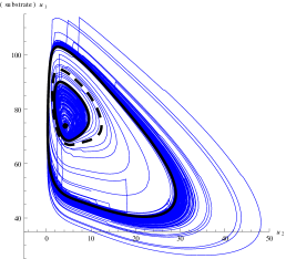
(a) (b)

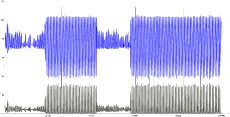
Figure 1: (a) Coexisting nested stable cycles in the model of an autocatalytic reaction by Moran and Goldbeter [35]. A heavy-tailed Lévy perturbation of the substrate input enables instant switchings between different ranges of substrate and product concentrations. (b) Random switching between periodic regimes of the substrate (blue) and the product (green) concentrations.

We perturb the parameter $v$ by a Lévy process $Z$ which is a compound Poisson process with the Pareto jump measure $\nu(dz)=\alpha z^{-1-\alpha}\mathbf{1}(z\geqslant 1)$, $\alpha>0$. We obtain the time scale rate

$$h_{\varepsilon}=\alpha\int_{z>\frac{1}{\varepsilon}}\frac{dz}{z^{1+\alpha}}=\varepsilon^{\alpha},\quad 0<\varepsilon<1.$$

and the limiting self-similar Radon measure

$$\mu(dz)=\alpha\frac{\mathbf{1}(z>0)}{z^{1+\alpha}}\,dz,\quad\alpha>0.$$

On the time scale $\frac{t}{\varepsilon^{\alpha}}$, transitions between the cycles occur according to a law of the Markov chain $m$ on the state space $\{\text{i},\text{o}\}$ with the generator

$$\mathcal{Q}=\begin{pmatrix}-Q^{\text{i}}&\leavevmode\nobreak\ Q^{\text{i}}\\ \leavevmode\nobreak\ Q^{\text{o}}&-Q^{\text{o}}\end{pmatrix}$$

where

$$Q^{\text{i}}:=\frac{\alpha}{\mathcal{T}_{\text{i}}}\int_{0}^{\mathcal{T}_{\text{i}}}\int_{1}^{\infty}\frac{\mathbf{1}_{D_{\text{o}}}(z-\varphi_{\text{i}}^{1}(s))}{|z-\varphi_{\text{i}}^{1}(s)|^{1+\alpha}}\,dz\,ds\quad\text{and}\quad Q^{\text{o}}:=\frac{\alpha}{\mathcal{T}_{\text{o}}}\int_{0}^{\mathcal{T}_{\text{o}}}\int_{1}^{\infty}\frac{\mathbf{1}_{D_{\text{i}}}(z-\varphi_{\text{o}}^{1}(s))}{|z-\varphi_{\text{o}}^{1}(s)|^{1+\alpha}}\,dz\,ds.$$

It is clear from the phase portrait of the system $\dot{u}=f(u)$ that the area of the attraction basin $D_{\text{i}}$ is much smaller than the area of $D_{\text{o}}$ and thus $Q^{\text{o}}\ll Q^{\text{i}}$. Consequently, the system will spend most of the time in the vicinity of one of the stable cycles, preferably near the outer one, see Fig. 1(b). Any concrete measurement of concentrations will yield a random variable with the law $P^{\text{i}}$ or $P^{\text{o}}$ supported on the cycles, see (2).

3 Proof

3.1 Preliminary results on the asymptotic first exit time

The proof of the main Theorem 2.2 is based on a result about the first exit times of a perturbed system from a domain $D$ around an attractor formulated in Theorem 2.1 in [21]. This result holds for deterministic vector fields $f$ which are inward pointing at the boundary of the bounded domain $D$. For general Morse–Smale systems this condition turn out to be too restrictive, since the boundary of domains of attraction $D^{\iota}$ is typically characteristic, that is the vector field close to the separating manifold acts tangentially. Hence there are trajectories in the domain $D^{\iota}$ which may stay close to the separatrix for an uncontrollably long time until they eventually converge to the attractor. The proof of the Theorem 2.1 in [21] does not use precisely that the vector field is inward pointing, but rather the implication that a small reduction of the domain of attraction is still positively invariant and that all trajectories starting in the reduced domain are close to the attractor all together in time.

Here we present another construction of the reduced domains of attraction which is applicable to our setting. It aims at avoiding the very slow dynamics near the characteristic boundary of the domain of attraction and will not change the essential behavior of the stochastic system. An analogous construction had been carried out in Chapter 2.2.1 of [12], for parabolic PDEs in the context of analysis of perturbed reaction-diffusion equations, with the additional difficulty that the latter do not have a backward flow.

We fix $R>0$ and $\delta>0$ and consider the $\delta$-tube around the boundary $\partial D^{\iota}$ intersected with $D^{\iota}\cap\mathcal{I}_{R}$, namely

$$\mathcal{M}^{\iota,R}_{\delta}:=\bigcup_{y\in\partial D^{\iota}}B_{\delta}(y)\cap D^{\iota}\cap\mathcal{I}_{R}.$$

Then the set

$$\mathbb{M}^{\iota,R}_{\delta}:=\bigcup_{t\geqslant 0}\varphi_{-t}(\mathcal{M}^{\iota,R}_{\delta})$$

denotes all initial values $x$ such that for some time $t\geqslant 0$ the forward flow $\varphi_{t}(x)$ enters $\mathcal{M}^{\iota,R}_{\delta}$. We define the flow-adapted reduced domain of attraction

$$D^{\iota,R}_{\delta}:=(D^{\iota}\cap\mathcal{I}_{R})\setminus\mathbb{M}^{\iota,R}_{\delta}.$$

For $\delta^{\prime}>0$, iterating this procedure by replacing $D^{\iota,R}$ by $D^{\iota,R}_{\delta}$ and obtain further reductions

$$\mathcal{M}^{\iota,R}_{\delta,\delta^{\prime}} :=\bigcup_{y\in\partial D^{\iota,R}_{\delta}}B_{\delta^{\prime}}(y)\cap D^{\iota,R}_{\delta},$$

$$\mathbb{M}^{\iota,R}_{\delta,\delta^{\prime}} :=\bigcup_{t\geqslant 0}\varphi_{-t}(\mathcal{M}^{\iota,R}_{\delta,\delta^{\prime}}),$$

$$D^{\iota,R}_{\delta,\delta^{\prime}} :=(D^{\iota}\cap\mathcal{I}_{R})\setminus\mathbb{M}^{\iota,R}_{\delta,\delta^{\prime}}.$$

The reduced domains $D^{\iota,R}_{\delta}$ and $D^{\iota,R}_{\delta,\delta^{\prime}}$ enjoy the following important properties.

Lemma 3.1.

Denote

$$\delta_{0}:=\frac{1}{2}\min_{1\leqslant\iota\leqslant\kappa}\operatorname{dist}\Big{(}K^{\iota},\displaystyle\bigcup_{\iota=1}^{\kappa}\partial D^{\iota}\Big{)},\quad\text{and}\quad\displaystyle R_{0}:=\inf\Big{\{}r>0\colon\bigcup_{\iota=1}^{\kappa}K^{\iota}\subset B_{r}(0)\Big{\}},$$

and let $\iota\in\{1,\dots,\kappa\}$ be fixed.

1. If $0<\delta<\delta_{0}$ and $R>R_{0}$, then $\varphi_{t}(D^{\iota,R}_{\delta})\subset D^{\iota,R}_{\delta}$ for all $t\geqslant 0$.

2. If $0<\delta<\delta_{0}$, $R>R_{0}$, and additionally $0<\gamma<\delta_{0}$, then there is $T^{*}=T^{*}_{\delta,R,\gamma}>0$ such that for all $x\in D^{\iota,R}_{\delta}$ and $t\geqslant T^{*}$

   $$u(t;x)\in B_{\gamma}(K^{\iota}).$$

   This property corresponds to Remark 2.1 in [21].

3. If $0<\delta<\delta^{\prime}<\delta_{0}$ and $R>R_{0}$, then $D^{\iota,R}_{\delta^{\prime}}\subset D^{\iota,R}_{\delta}$.

4. If $\delta,\delta^{\prime}>0$ such that $\delta+\delta^{\prime}<\delta_{0}$ and $R>R_{0}$, then $\varphi_{t}(D^{\iota,R}_{\delta,\delta^{\prime}})\subset D^{\iota,R}_{\delta,\delta^{\prime}}$ for all $t\geqslant 0$.

5. If $\delta,\delta^{\prime},\delta^{\prime\prime}>0$ with $\delta^{\prime}<\delta^{\prime\prime}$ and $\delta+\delta^{\prime\prime}<\delta_{0}$, then $D^{\iota,R}_{\delta,\delta^{\prime}}\subset D^{\iota,R}_{\delta,\delta^{\prime\prime}}$.

6. We have

   $$\bigcup_{\begin{subarray}{c}\delta,\delta^{\prime}>0\\ \delta+\delta^{\prime}<\delta_{0}\end{subarray}}D^{\iota,R}_{\delta,\delta^{\prime}}=D^{\iota}\cap\mathcal{I}_{R}.$$

The proof of the Lemma is rather straightforward and postponed to the Appendix.

Under an appropriate choice of parameters $R$, $\delta$, $\delta^{\prime}$, $x\in D^{\iota,R}_{\delta,\delta^{\prime}}$, $\varepsilon>0$ and $\iota\in\{0,\dots,\kappa\}$ we define the time

$$\mathbb{T}_{x}^{\iota,R}(\varepsilon):=\inf\{t>0\colon X^{\varepsilon}_{t,x}\notin D^{\iota,R}_{\delta}\}.$$

The next Theorem 3.2 is based on the Theorem 2.1 in [21] and deals with the behavior of $\mathbb{T}_{x}^{\iota,R}(\varepsilon)$ in the limit of small $\varepsilon$. We will use the following version of Theorem 2.1 in [21] slightly adapted to our setting.

Theorem 3.2 (The exit problem of $X^{\varepsilon}$).

Let Hypotheses (D.1) and (S.1-2) be fulfilled. Choose $R>R_{0}$, $\iota\in\{1,\dots,\kappa\}$ and $\delta,\delta^{\prime}>0$ with $\delta+\delta^{\prime}<\delta_{0}$. If $Q^{\iota}(\partial D^{\iota,R}_{\delta})=0$ and $Q^{\iota}((D^{\iota,R}_{\delta})^{c})>0$, then we have for any $\theta>0$ and $U\in\mathfrak{B}(\mathbb{R}^{d})$ satisfying $Q(\partial U)=0$ that

$$\lim_{\varepsilon\to 0}\sup_{y\in D^{\iota,R}_{\delta,\delta^{\prime}}}\Big{|}\mathbb{E}_{y}\Big{[}e^{-\theta Q((D^{\iota,R}_{\delta})^{c})h_{\varepsilon}\mathbb{T}^{\iota,R}(\varepsilon)}\mathbf{1}\{X^{\varepsilon}_{\mathbb{T}^{\iota,R}(\varepsilon)}\in U\}\Big{]}-\frac{1}{1+\theta}\frac{Q\big{(}U\cap(D^{\iota,R}_{\delta})^{c}\big{)}}{Q\big{(}(D^{\iota,R}_{\delta})^{c}\big{)}}\Big{|}=0.$$ (16)

This result implies that under the previous assumptions the first exit times and the first exit location behave as

$$h_{\varepsilon}\;Q^{\iota}((D^{\iota,R}_{\delta})^{c})\;\mathbb{T}_{x}^{\iota,R}(\varepsilon)\stackrel{{\scriptstyle d}}{{\longrightarrow}}\mbox{EXP}(1),$$

$$\mathbb{P}_{x}\Big{(}X_{\mathbb{T}^{\iota,R}(\varepsilon)}^{\varepsilon}\in U\Big{)}\to\frac{Q^{\iota}\big{(}U\cap(D^{\iota,R}_{\delta})^{c}\big{)}}{Q^{\iota}\big{(}(D^{\iota,R}_{\delta})^{c}\big{)}},$$

in the limit $\varepsilon\to 0$, where the convergence is uniform over all initial values $x\in D^{\iota,R}_{\delta,\delta^{\prime}}$. These results allow the construction of a jump process, which converges weakly to an approximating continuous time Markov chain $m$ with the generator (13).

3.2 Proof of Theorem 2.2

Fix the error constant $\delta^{*}>0$. In the first step we fix the parameters $R$, $\delta$ and $\delta^{\prime}$ accordingly and construct an approximating Markov chain.

1. Approximating Markov chains.

The limiting measure $\mu$ of the regularly varying Lévy measure $\nu$ given in (3) is a Radon measure. We recall the definition of $R_{0}$ in Lemma 3.1. We may fix a radius $R>R_{0}$, depending only on $\delta^{*}$, such that

$$\max_{\iota=1,\dots,\kappa}Q^{\iota}(\mathcal{I}_{R}^{c})<\frac{\delta^{*}}{2}.$$

In addition, by compactness of $\mathcal{I}_{R}$ we may fix one after the other, $\delta>0$ and $\delta^{\prime}>0$, with $\delta+\delta^{\prime}<\delta_{0}=\frac{1}{2}\min_{\iota=1,\dots,\kappa}\min\{\operatorname{dist}(K^{\iota},\partial D^{\iota}),\operatorname{dist}(x,\mathcal{D}^{\iota})\}$ such that

$$\max_{\iota=1,\dots,\kappa}Q^{\iota}\Big{(}\mathcal{I}_{R}\setminus\bigcup_{\ell=1}^{\kappa}D^{\ell,R}_{\delta,\delta^{\prime}}\Big{)}<\frac{\delta^{*}}{2},$$

where $\delta=\delta(R,\delta^{*})$ and $\delta^{\prime}=\delta^{\prime}(R,\delta^{*},\delta)$. Combining the previous two inequalities we obtain that

$$\max_{\iota=1,\dots,\kappa}Q^{\iota}\Big{(}\mathbb{R}^{d}\backslash\bigcup_{\ell=1}^{\kappa}D^{\ell,R}_{\delta,\delta^{\prime}}\Big{)}<\delta^{*}.$$ (17)

We lighten the notation. For $\delta^{*}>0$ and the dependent parameters $R$, $\delta$, and $\delta^{\prime}$ fixed we write shorthand $\widehat{D}^{\iota}=D^{\iota,R}_{\delta}$ and $\widetilde{D}^{\iota}=D^{\iota,R}_{\delta,\delta^{\prime}}$. Furthermore we use $A^{c}:=\mathbb{R}^{d}\setminus A$ for any $A\subset\mathbb{R}^{d}$.

Denote by $m^{\delta^{*}}=(m^{\delta^{*}})_{t\geqslant 0}$ a continuous time Markov chain with values in the set of indices $\{1,\dots,\kappa\}\cup\{0\}$ enlarged by the absorbing cemetery state $0$ with the generator $\mathcal{Q}^{\delta^{*}}$ given by

$$\mathcal{Q}^{\delta^{*}}:= \left(\begin{array}[]{ccccc}-Q^{1}\left(\big{(}\widehat{D}^{1}\big{)}^{c}\right)&Q^{1}\left(\widetilde{D}^{2}\right)&\dots&Q^{1}\left(\widetilde{D}^{\kappa}\right)&\displaystyle Q^{1}\Big{(}\big{(}\widehat{D}^{1}\cup\bigcup_{\iota=2}^{\kappa}\widetilde{D}^{\iota}\big{)}^{c}\Big{)}\\ \vdots&&&\vdots\\ Q^{\kappa}\left(\widetilde{D}^{1}\right)&\dots&Q^{\kappa}\left(\widetilde{D}^{\kappa-1}\right)&-Q^{\kappa}\Big{(}\big{(}\widehat{D}^{\iota_{\kappa}}\big{)}^{c}\Big{)}&\displaystyle Q^{\kappa}\Big{(}\big{(}\widehat{D}^{\kappa}\cup\bigcup_{\iota=1}^{\kappa-1}\widetilde{D}^{\iota}\big{)}^{c}\Big{)}\\[5.69054pt] 0&0&\dots&0&0\end{array}\right).$$

For $\mathcal{Q}$ defined in (13) we construct the matrix

$$\mathcal{Q}^{0}:=\begin{pmatrix}\mathcal{Q}&0\\ 0&0\end{pmatrix}$$

and denote by $m^{0}$ a continuous-time Markov chain on the state space $\{1,\dots,\kappa\}\cup\{0\}$ with the generator $\mathcal{Q}^{0}$. As a consequence of (17) we have

$$\max_{i,j}|\mathcal{Q}^{\delta^{*}}(i,j)-\mathcal{Q}^{0}(i,j)|<\delta^{*}.$$

This implies that $m^{\delta^{*}}\rightarrow m^{0}$ as $\delta^{*}\searrow 0$ in the sense of finite dimensional distributions. Note that the transition rate to the cemetery state $0$ tends to $0$ as $\delta^{*}\searrow 0$ due to (17).

2. Transition probabilities.

Let $N\geqslant 1$, $\iota_{0},\dots,\iota_{N}\in\{1,\dots,\kappa\}\cup\{0\}$, $x\in\widetilde{D}^{\iota}$ and $0<s_{1}<\dots<s_{N}$. Let us show that

$$\lim_{\varepsilon\rightarrow 0+}\mathbb{P}_{x}\Big{(}X^{\varepsilon}_{\frac{s_{1}}{h_{\varepsilon}}}\in\widetilde{D}^{\iota_{1}},\dots,X^{\varepsilon}_{\frac{s_{N}}{h_{\varepsilon}}}\in\widetilde{D}^{\iota_{N}}\Big{)}=\mathbb{P}_{\iota_{0}}(m^{\delta^{*}}_{s_{1}}=\iota_{1},\dots,m^{\delta^{*}}_{s_{N}}=\iota_{N}).$$ (18)

Since $0$ is an absorbing state, we can restrict ourselves to the states $\{1,\dots,\kappa\}$. We first construct an approximating jump process with the help of Theorem 3.2 and define recursively the arrival times $\{T_{n}^{\varepsilon}\}_{n\geqslant 0}$ and the random states $\{S_{n}^{\varepsilon}\}_{n\geqslant 0}$ taking values in $\{0,\dots,\kappa\}\cup\{0\}$. We fix the initial time and state

$$T_{0}^{\varepsilon}:=0,\qquad S_{0}^{\varepsilon}:=\sum_{\ell=1}^{\kappa}\ell\cdot\mathbf{1}_{\widetilde{D}^{\ell}}(x).$$

For $n\in\mathbb{N}$ we set

$$T_{n+1}^{\varepsilon}:=\begin{cases}\displaystyle\inf\Big{\{}t>T_{n}^{\varepsilon}\colon X^{\varepsilon}_{t,x}\in\bigcup_{\begin{subarray}{c}\ell=1\\ \ell\neq S_{n}\end{subarray}}^{k}\widetilde{D}^{\ell}\Big{\}},&\displaystyle\mbox{ if }S_{n}^{\varepsilon}\in\bigcup_{\ell=1}^{\kappa}\widetilde{D}^{\ell},\\ \infty,&\displaystyle\mbox{ if }S_{n}^{\varepsilon}\notin\bigcup_{\ell=1}^{\kappa}\widetilde{D}^{\ell},\end{cases}$$

$$S_{n+1}^{\varepsilon}:=\begin{cases}\displaystyle\sum_{\ell=1}^{\kappa}\ell\cdot\mathbf{1}_{\widetilde{D}^{\ell}}(X^{\varepsilon}_{T_{n+1},x}),&\displaystyle\mbox{ if }T_{n+1}^{\varepsilon}<\infty,\\ \displaystyle 0,&\displaystyle\mbox{ if }T_{n+1}^{\varepsilon}=\infty.\end{cases}$$

We define the approximating jump process

$$M^{\varepsilon,\delta^{*}}_{t}:=\sum_{n=0}^{\infty}S_{n}^{\varepsilon}\cdot\mathbf{1}\big{\{}T_{n}^{\varepsilon}\leqslant\frac{t}{h_{\varepsilon}}<T_{n+1}^{\varepsilon}\big{\}}.$$

The convergence in (18) can be expressed conveniently in terms of $M^{\varepsilon,\delta^{*}}$ as follows

$$\lim_{\varepsilon\rightarrow 0+}\mathbb{P}_{x}\Big{(}M^{\varepsilon,\delta^{*}}_{\frac{s_{1}}{h_{\varepsilon}}}=\iota_{1},\dots,M^{\varepsilon,\delta^{*}}_{\frac{s_{N}}{h_{\varepsilon}}}=\iota_{N}\Big{)}=\mathbb{P}_{\iota_{0}}(m^{\delta^{*}}_{s_{1}}=\iota_{1},\dots,m^{\delta^{*}}_{s_{N}}=\iota_{N}).$$ (19)

Following for instance Lemma 2.12 and Lemma 2.13 in Xia [45], the convergence

$$M^{\varepsilon,\delta^{*}}\to m^{\delta^{*}}\quad\mbox{ as }\varepsilon\to 0$$

in the sense of finite dimensional distributions it is equivalent to convergence

$$(T_{k}^{\varepsilon},S_{k}^{\varepsilon})_{0\leqslant k\leqslant n}\stackrel{{\scriptstyle d}}{{\longrightarrow}}(T_{k},S_{k})_{0\leqslant k\leqslant n},$$

for any $n\in\mathbb{N}$, where $T_{k}$ is the $k$-th arrival time for the Markov chain $m^{\delta^{*}}$ and $S_{k}=m^{\delta^{*}}_{\tau_{k}}$. This is equivalent to the following statement. For indices $\iota_{0},\iota_{1},\dots\iota_{n}\in\{1,\dots,\kappa\}$, with $\iota_{k}\neq\iota_{k+1}$, $k\in\{0,\dots,n-1\}$, $u_{1},\dots,u_{n}\geqslant 0$, and an initial value $x\in\widetilde{D}^{\iota_{0}}$ we have

$$\mathbb{E}_{x}\Big{[}e^{-u_{1}T_{1}^{\varepsilon}-\dots-u_{n}(T_{n}^{\varepsilon}-T_{n-1}^{\varepsilon})}\cdot \mathbf{1}\{S_{1}^{\varepsilon}=\iota_{1},\dots,S_{n}^{\varepsilon}=\iota_{n}\}\Big{]}$$

$$\qquad\stackrel{{\scriptstyle\varepsilon\to 0}}{{\longrightarrow}}\prod_{j=0}^{n-1}\frac{Q^{\iota_{j}}\big{(}(\widehat{D}^{\iota_{j}})^{c}\big{)}}{Q^{\iota_{j}}\big{(}(\widehat{D}^{\iota_{j}})^{c}\big{)}+u_{j+1}}\cdot\frac{Q^{\iota_{j}}\big{(}\widetilde{D}^{\iota_{j+1}}\big{)}}{Q^{\iota_{j}}\big{(}(\widehat{D}^{\iota_{j}})^{c}\big{)}}.$$ (20)

This implies the desired convergence of finite dimensional distributions (19). To prove the convergence in (20) we use the strong Markov property of $X^{\varepsilon}$ for the following recursive estimate

$$\mathbb{E}_{x}\Big{[}e^{-u_{1}T_{1}^{\varepsilon}-\dots-u_{n}(T_{n}^{\varepsilon}-T_{n-1}^{\varepsilon})}\cdot\mathbf{1}\{S_{1}^{\varepsilon}=\iota_{1},\dots,S_{n}^{\varepsilon}=\iota_{n}\}\Big{]}$$

$$=\mathbb{E}_{x}\Big{[}\mathbb{E}\Big{[}e^{-u_{1}T_{1}^{\varepsilon}-\dots-u_{n}(T_{n}^{\varepsilon}-T_{n-1}^{\varepsilon})}\cdot\mathbf{1}\{S_{1}^{\varepsilon}=\iota_{1},\dots,S_{n}^{\varepsilon}=\iota_{n}\}\Big{|}\mathcal{F}_{T_{1}^{\varepsilon}}\Big{]}\Big{]}$$

$$=\mathbb{E}_{x}\Big{[}e^{-u_{1}T_{1}^{\varepsilon}}\cdot\mathbf{1}\{S_{1}^{\varepsilon}=\iota_{1}\}\mathbb{E}\Big{[}e^{-u_{2}(T_{2}^{\varepsilon}-T_{1}^{\varepsilon})-\dots-u_{n}(T_{n}^{\varepsilon}-T_{n-1}^{\varepsilon})}\cdot\mathbf{1}\{S_{1}^{\varepsilon}=\iota_{2},\dots,S_{n}^{\varepsilon}=\iota_{n}\}\Big{|}\mathcal{F}_{T_{1}^{\varepsilon}}\Big{]}\Big{]}$$

$$=\mathbb{E}_{x}\Big{[}e^{-u_{1}T_{1}^{\varepsilon}}\cdot\mathbf{1}\{X^{\varepsilon}_{T_{1}^{\varepsilon}}\in\widetilde{D}^{\iota_{1}}\}\;\mathbb{E}_{X^{\varepsilon}_{T_{1}^{\varepsilon}}}\Big{[}e^{-u_{2}(T_{2}^{\varepsilon}-T_{1}^{\varepsilon})-\dots-u_{n}(T_{n}^{\varepsilon}-T_{n-1}^{\varepsilon})}\cdot\mathbf{1}\{S_{1}^{\varepsilon}=\iota_{2},\dots,S_{n}^{\varepsilon}=\iota_{n}\}\Big{]}\Big{]}$$

$$\leqslant\mathbb{E}_{x}\Big{[}e^{-u_{1}T_{1}^{\varepsilon}}\cdot\mathbf{1}\{X^{\varepsilon}_{T_{1}^{\varepsilon}}\in\widetilde{D}^{\iota_{1}}\}\Big{]}\sup_{y\in\widetilde{D}^{\iota_{1}}}\mathbb{E}_{y}\Big{[}e^{-u_{2}T_{1}^{\varepsilon}-\dots-u_{n}(T_{n-1}^{\varepsilon}-T_{n-2}^{\varepsilon})}\cdot\mathbf{1}\{S_{1}^{\varepsilon}=\iota_{2},\dots,S_{n}^{\varepsilon}=\iota_{n}\}\Big{]}.$$

We iterate the preceding argument $n-2$ times and obtain the estimate

$$\mathbb{E}_{x}\Big{[}e^{-u_{1}T_{1}^{\varepsilon}-\dots-u_{n}(T_{n}^{\varepsilon}-T_{n-1}^{\varepsilon})}\cdot\mathbf{1}\{S_{1}^{\varepsilon}=\iota_{1},\dots,S_{n}^{\varepsilon}=\iota_{n}\}\Big{]}$$

$$\leqslant\mathbb{E}_{x}\Big{[}e^{-u_{1}T_{1}^{\varepsilon}}\cdot\mathbf{1}\{X^{\varepsilon}_{T_{1}^{\varepsilon}}\in\widetilde{D}^{\iota_{1}}\}\Big{]}\prod_{\ell=1}^{n-1}\sup_{y\in\widetilde{D}^{\iota_{\ell}}}\mathbb{E}_{y}\Big{[}e^{-u_{\ell}T_{1}^{\varepsilon}}\cdot\mathbf{1}\{X^{\varepsilon}_{T_{1}^{\varepsilon}}\in\widetilde{D}^{\iota_{\ell+1}}\}\Big{]}.$$

The same reasoning holds true for the estimate from below if we change -mutatis mutandis- the supremum by the infimum. The limit (16) in Theorem 3.2 states that

$$\sup_{y\in\widetilde{D}^{\iota_{\ell}}}\mathbb{E}_{y}\Big{[}e^{-u_{\ell}T_{1}^{\varepsilon}}\cdot\mathbf{1}\{X^{\varepsilon}_{T_{1}^{\varepsilon}}\in\widetilde{D}^{\iota_{\ell+1}}\}\Big{]}\stackrel{{\scriptstyle\varepsilon\to 0}}{{\longrightarrow}}\frac{Q^{\iota_{j}}\big{(}(\widehat{D}^{\iota_{j}})^{c}\big{)}}{Q^{\iota_{j}}\big{(}(\widehat{D}^{\iota_{j}})^{c}\big{)}+u_{j+1}}\cdot\frac{Q^{\iota_{j}}(\widetilde{D}^{\iota_{j+1}})}{Q^{\iota_{j}}\big{(}(\widehat{D}^{\iota_{j}})^{c}\big{)}}.$$

This shows the desired convergence in (20) and finishes the proof of (19). Statement 1. of Theorem 2.2 is proved.

3. Location of $X^{\varepsilon}$ on the attractor.

We prove the second statement of the Theorem 2.2. Since $X^{\varepsilon}$ is a strong Markov process, it is enough to prove the result for $s=0$ and $x\in\widetilde{D}^{\iota}$, namely that

$$\lim_{\varepsilon\rightarrow 0+}\mathbb{E}_{x}\Big{[}\psi(X^{\varepsilon}_{\frac{t}{h_{\varepsilon}},x})\Big{]}=\mathbb{E}_{\iota}\Big{[}\int_{\mathbb{R}^{d}}\psi(v)\,dP^{m^{\delta}_{t}}(v)\Big{]}.$$

Indeed, the Markov property of $X^{\varepsilon}$ yields

$$\mathbb{E}_{x}\Big{[}\psi(X^{\varepsilon}_{\frac{t+\sigma r_{\varepsilon}}{h_{\varepsilon}}})\Big{]} =\mathbb{E}_{x}\Big{[}\frac{h_{\varepsilon}}{2r_{\varepsilon}}\int_{-\frac{r_{\varepsilon}}{h_{\varepsilon}}}^{\frac{r_{\varepsilon}}{h_{\varepsilon}}}\psi(X^{\varepsilon}_{\frac{t+s}{h_{\varepsilon}}})ds\Big{]}$$

$$=\mathbb{E}_{x}\Big{[}\mathbb{E}\Big{[}\frac{h_{\varepsilon}}{2r_{\varepsilon}}\int_{-\frac{r_{\varepsilon}}{h_{\varepsilon}}}^{\frac{r_{\varepsilon}}{h_{\varepsilon}}}\psi(X^{\varepsilon}_{\frac{t+s}{h_{\varepsilon}}})\,ds\Big{|}\mathcal{F}_{\frac{t-r_{\varepsilon}}{h_{\varepsilon}}}\Big{]}\Big{]}$$

$$=\mathbb{E}_{x}\Big{[}\mathbb{E}_{X^{\varepsilon}_{\frac{t-r_{\varepsilon}}{h_{\varepsilon}}}}\Big{[}\frac{h_{\varepsilon}}{2r_{\varepsilon}}\int_{0}^{\frac{2r_{\varepsilon}}{h_{\varepsilon}}}\psi(X^{\varepsilon}_{s})\,ds\Big{]}\Big{]}$$

$$\leqslant\sum_{\iota=1}^{\kappa}\mathbb{E}_{x}\Big{[}\mathbb{E}_{X^{\varepsilon}_{\frac{t-r_{\varepsilon}}{h_{\varepsilon}}}}\Big{[}\frac{h_{\varepsilon}}{2r_{\varepsilon}}\int_{0}^{\frac{2r_{\varepsilon}}{h_{\varepsilon}}}\psi(X^{\varepsilon}_{s})\,ds\Big{]}\cdot\mathbf{1}_{\widetilde{D}^{\iota}}(X^{\varepsilon}_{\frac{t-r_{\varepsilon}}{h_{\varepsilon}}})\Big{]}+\|\psi\|_{\infty}\delta^{*}$$

$$\leqslant\sum_{\iota=1}^{\kappa}\sup_{y\in\widetilde{D}^{\iota}}\mathbb{E}_{y}\Big{[}\frac{h_{\varepsilon}}{2r_{\varepsilon}}\int_{0}^{\frac{2r_{\varepsilon}}{h_{\varepsilon}}}\psi(X^{\varepsilon}_{s})\,ds\Big{]}\cdot\mathbb{P}_{x}\Big{(}X^{\varepsilon}_{\frac{t-r_{\varepsilon}}{h_{\varepsilon}}}\in\widetilde{D}^{\iota}\Big{)}+\|\psi\|_{\infty}\delta^{*}.$$ (21)

We treat the two factors of the summands separately.

Lemma 3.3.

Let $\delta^{*}$, $\delta^{\prime}$, $\delta>0$ and $R>R_{0}$ be chosen as above. If $0<\gamma<\delta_{0}$, $\psi\in\mathcal{C}_{b}(\mathbb{R}^{d},\mathbb{R})$ and $\iota\in\{1,\dots,\kappa\}$ then there is a constant $\varepsilon_{0}>0$ such that for any $\varepsilon\in(0,\varepsilon_{0}]$

$$\sup_{y\in D^{\iota,R}_{\delta,\delta^{\prime}}}\Big{|}\mathbb{E}_{y}\Big{[}\frac{h_{\varepsilon}}{2r_{\varepsilon}}\int_{0}^{\frac{2r_{\varepsilon}}{h_{\varepsilon}}}\psi(X^{\varepsilon}_{s})\,ds\Big{]}-\int_{K^{\iota}}\psi(v)\,dP^{\iota}(v)\Big{|}\leqslant\gamma.$$

Proof.

Fix $0<\gamma<\delta_{0}$. For convenience we return to the abbreviation $\widetilde{D}^{\iota}$. The local ergodicity condition (2) of the deterministic dynamical system ensures the existence of a constant $\mathcal{T}^{*}>0$ such that for all $\mathcal{T}\geqslant\mathcal{T}^{*}$

$$\max_{\iota\in\{1,\dots,\kappa\}}\sup_{y\in\overline{\widetilde{D}^{\iota}}}\Big{|}\frac{1}{\mathcal{T}}\int_{0}^{\mathcal{T}}\psi(\varphi_{s}(y))\,ds-\int_{K^{\iota}}\psi(v)\,dP^{\iota}(v)\Big{|}<\frac{\gamma}{3}.$$

According to Lemma 3.1.1.(b) there is a constant $T^{*}>0$ depending on $R,\delta$ and $\gamma$ which ensures that for all $y\in\widetilde{D}^{\iota}$ and $t\geqslant T^{*}$

$$\operatorname{dist}(\varphi_{t}(y),\partial\widetilde{D}^{\iota})>\delta_{0}.$$

We choose $\mathcal{T}^{*}\geqslant T^{*}$ without loss of generality. Denote by $\ell_{\varepsilon}:=\lfloor 2r_{\varepsilon}/h_{\varepsilon}\mathcal{T}^{*}\rfloor$ the maximal number of times how often $\mathcal{T}^{*}$ fits into $2r_{\varepsilon}/h_{\varepsilon}$. Then $\mathcal{T}_{\varepsilon}:=2r_{\varepsilon}/h_{\varepsilon}\ell_{\varepsilon}$ satisfies $\mathcal{T}^{*}\leqslant\mathcal{T}_{\varepsilon}<2\mathcal{T}^{*}$ for any $\varepsilon>0$. It is well-known that for any $\rho\in(0,1)$ and $\varepsilon>0$ the random variable

$$\tau:=\inf\{t>0\colon|\Delta_{t}Z|>\varepsilon^{-\rho}\}$$

is exponentially distributed with parameter $\nu(B_{\varepsilon^{-\rho}}^{c}(0))$ and that it is independent of the process of $(Z_{t})_{0\leqslant t<\tau}$ and hence $(X^{\varepsilon}_{t})_{0\leqslant t<\tau}$. Since by the regular variation of $\nu$ we have $\nu(B_{\varepsilon^{-\rho}}^{c}(0))/\varepsilon^{-\alpha\rho}\mu(B_{1}^{c}(0))\rightarrow 1$ as $\varepsilon\rightarrow 0$, there exists a constant $\rho_{0}\in(0,1)$ such that for any $\rho\in(0,\rho_{0}]$

$$\mathbb{P}\big{(}\tau>\frac{2r_{\varepsilon}}{h_{\varepsilon}}\big{)}=\exp\big{(}-\frac{2r_{\varepsilon}\nu(B_{\varepsilon^{-\rho}}^{c}(0))}{h_{\varepsilon}}\big{)}\to 1\quad\mbox{ as }\varepsilon\to 0.$$

In particular, we may choose the upper bounds $\rho_{0},\varepsilon_{0}\in(0,1)$ such that for all $\varepsilon\in(0,\varepsilon_{0}]$ and $\rho\in(0,\rho_{0}]$ we have $1-\exp(-2r_{\varepsilon}\nu(B_{\varepsilon^{-\rho}}^{c}(0))/h_{\varepsilon})<\gamma/3\|\psi\|_{\infty}$. For convenience we denote by $\widetilde{\mathbb{P}}$ and $\widetilde{\mathbb{E}}$ the probability measure $\mathbb{P}(\,\cdot\,|\tau>2r_{\varepsilon}/h_{\varepsilon})$ and its expectation. We may assume without loss of generality that $\psi$ is uniformly continuous on $\mathbb{R}^{d}$, we denote its modulus of continuity by $\varpi_{\psi}$. Since $\varphi_{\psi}(\beta)\rightarrow 0$ as $\beta\rightarrow 0$, we may choose $\beta_{0}\in(0,1)$ such that for all $\beta\in(0,\beta_{0}]$ we have $\varpi(\beta)\leqslant\gamma/3$. For fixed $\beta\in(0,\beta_{0}]$ we apply Corollary 3.1 in [21] for the upper bound $2\mathcal{T}^{*}$ of $\mathcal{T}_{\varepsilon}$, which provides the existence of constants $p_{0},\varepsilon_{0}\in(0,1)$ such that for all $p\in(0,p_{0}]$ and $\varepsilon\in(0,\varepsilon_{0}]$

$$\widetilde{\mathbb{E}}_{y}\Big{[}\frac{h_{\varepsilon}}{2r_{\varepsilon}}\int_{0}^{\ell_{\varepsilon}\mathcal{T}_{\varepsilon}}\psi(X^{\varepsilon}_{s})\,ds\Big{]}=\frac{h_{\varepsilon}}{2r_{\varepsilon}}\widetilde{\mathbb{E}}_{y}\Big{[}\int_{0}^{\mathcal{T}_{\varepsilon}}\psi(X^{\varepsilon}_{s})\,ds+\int_{\mathcal{T}_{\varepsilon}}^{\ell_{\varepsilon}\mathcal{T}_{\varepsilon}}\psi(X^{\varepsilon}_{s})\,ds\Big{]}$$ (22)

$$\leqslant\frac{h_{\varepsilon}}{2r_{\varepsilon}}\widetilde{\mathbb{E}}_{y}\Big{[}\Big{(}\int_{0}^{\mathcal{T}_{\varepsilon}}\psi(X^{\varepsilon}_{s})\,ds+\int_{\mathcal{T}_{\varepsilon}}^{\ell_{\varepsilon}\mathcal{T}_{\varepsilon}}\psi(X^{\varepsilon}_{s})\,ds\Big{)}\mathbf{1}\Big{\{}\sup_{s\in[0,\mathcal{T}_{\varepsilon}]}\|X^{\varepsilon}_{s}-\varphi_{s}(y)\|<\beta\Big{\}}\Big{]}+\|\psi\|_{\infty}e^{-\varepsilon^{-p}}$$

We continue with the first term. Recall that by construction $\ell_{\varepsilon}\mathcal{T}_{\varepsilon}=2r_{\varepsilon}/h_{\varepsilon}$. We are now in the position to apply the Markov property of $X^{\varepsilon}$ again and obtain the recursion

$$\frac{h_{\varepsilon}}{2r_{\varepsilon}}\widetilde{\mathbb{E}}_{y}\Big{[}\Big{(}\int_{0}^{\mathcal{T}_{\varepsilon}}\psi(X^{\varepsilon}_{s})\,ds+\int_{\mathcal{T}_{\varepsilon}}^{\ell_{\varepsilon}\mathcal{T}_{\varepsilon}}\psi(X^{\varepsilon}_{s})\,ds\Big{)}\mathbf{1}\Big{\{}\sup_{s\in[0,\mathcal{T}_{\varepsilon}]}\|X^{\varepsilon}_{s}-\varphi_{s}(y)\|<\beta\Big{\}}\Big{]}$$

$$=\frac{h_{\varepsilon}\mathcal{T}_{\varepsilon}}{2r_{\varepsilon}}\widetilde{\mathbb{E}}_{y}\Big{[}\frac{1}{\mathcal{T}_{\varepsilon}}\int_{0}^{\mathcal{T}_{\varepsilon}}\psi(X^{\varepsilon}_{s})\,ds\cdot\mathbf{1}\Big{\{}\sup_{s\in[0,\mathcal{T}_{\varepsilon}]}\|X^{\varepsilon}_{s}-\varphi_{s}(y)\|<\beta\Big{\}}\Big{]}$$

$$\qquad+\frac{h_{\varepsilon}}{2r_{\varepsilon}}\widetilde{\mathbb{E}}_{y}\Big{[}\widetilde{\mathbb{E}}_{X^{\varepsilon}_{\mathcal{T}_{\varepsilon}}}\Big{[}\int_{0}^{(\ell_{\varepsilon}-1)\mathcal{T}_{\varepsilon}}\psi(X^{\varepsilon}_{s})\,ds\Big{]}\cdot\mathbf{1}\{X^{\varepsilon}_{\mathcal{T}_{\varepsilon}}\in\widetilde{D}^{\iota}\}\Big{]}$$

$$\leqslant\frac{h_{\varepsilon}\mathcal{T}_{\varepsilon}}{2r_{\varepsilon}}\Big{(}\frac{1}{\mathcal{T}_{\varepsilon}}\int_{0}^{\mathcal{T}_{\varepsilon}}\psi(\varphi_{s}(y))\,ds+\varpi_{\psi}(\beta)\Big{)}+\frac{h_{\varepsilon}}{2r_{\varepsilon}}\sup_{z\in\widetilde{D}^{\iota}}\widetilde{\mathbb{E}}_{z}\Big{[}\int_{0}^{(\ell_{\varepsilon}-1)\mathcal{T}_{\varepsilon}}\psi(X^{\varepsilon}_{s})\,ds\Big{]}$$

$$\leqslant\frac{1}{\ell_{\varepsilon}}\Big{(}\int_{K^{\iota}}\psi(v)\,dP^{\iota}(dv)+\frac{\gamma}{3}\Big{)}+\sup_{z\in\widetilde{D}^{\iota}}\widetilde{\mathbb{E}}_{z}\Big{[}\frac{h_{\varepsilon}}{2r_{\varepsilon}}\int_{0}^{(\ell_{\varepsilon}-1)\mathcal{T}_{\varepsilon}}\psi(X^{\varepsilon}_{s})\,ds\Big{]}.$$

Iterating the step in (22) $\ell_{\varepsilon}-1$ times and choosing $\varepsilon_{0}\in(0,1)$ such that for all $\varepsilon\in(0,\varepsilon_{0}]$ we have $\ell_{\varepsilon}\|\psi\|_{\infty}\exp(-\varepsilon^{-p})<\gamma/3$ we obtain

$$\widetilde{\mathbb{E}}_{y}\Big{[}\frac{h_{\varepsilon}}{2r_{\varepsilon}}\int_{0}^{\ell_{\varepsilon}\mathcal{T}_{\varepsilon}}\psi(X^{\varepsilon}_{s})\,ds\Big{]} \leqslant\Big{(}\int_{K^{\iota}}\psi(v)\,dP^{\iota}(dv)+\frac{\gamma}{3}\Big{)}+\frac{\gamma}{3},$$

and eventually end up with

$$\mathbb{E}_{y}\Big{[}\frac{h_{\varepsilon}}{2r_{\varepsilon}}\int_{0}^{\frac{2r_{\varepsilon}}{h_{\varepsilon}}}\psi(X^{\varepsilon}_{s})\,ds\Big{]} \leqslant\widetilde{\mathbb{E}}_{y}\Big{[}\frac{h_{\varepsilon}}{2r_{\varepsilon}}\int_{0}^{\frac{2r_{\varepsilon}}{h_{\varepsilon}}}\psi(X^{\varepsilon}_{s})\,ds\Big{]}+\frac{\gamma}{3}$$

$$\leqslant\int_{K^{\iota}}\psi(v)\,dP^{\iota}(dv)+\gamma.$$

The lower estimate follows analogously. This finishes the proof. ∎

Lemma 3.4.

Let $\delta^{*}$, $\delta^{\prime}$, $\delta>0$ and $R>R_{0}$ be chosen as above. If $0<\gamma^{\prime}<\delta_{0}$ and $\iota\in\{1,\dots,\kappa\}$ then there is a constant $\varepsilon_{0}\in(0,1)$ such that for any $x\in D^{\iota}_{\delta,\delta^{\prime}}$ and $\varepsilon\in(0,\varepsilon_{0}]$

$$\mathbb{P}_{x}\Big{(}X^{\varepsilon}_{\frac{t-r_{\varepsilon}}{h_{\varepsilon}}}\in D^{\iota,R}_{\delta,\delta^{\prime}}\Big{)}\leqslant(1+\gamma^{\prime})\mathbb{P}_{x}\Big{(}X^{\varepsilon}_{\frac{t}{h_{\varepsilon}}}\in D^{\iota,R}_{\delta,\delta^{\prime}}\Big{)}.$$ (23)

Proof.

Fix $0<\gamma^{\prime}<\delta_{0}$. For convenience we return to the abbreviation $\widetilde{D}^{\iota}$. With the help of the Markov property we obtain

$$\mathbb{P}_{x}\Big{(}X^{\varepsilon}_{\frac{t}{h_{\varepsilon}}}\in\widetilde{D}^{\iota}\Big{)} =\sum_{\ell=1}^{\kappa}\mathbb{P}_{x}\Big{(}X^{\varepsilon}_{\frac{t-r_{\varepsilon}}{h_{\varepsilon}}}\in\widetilde{D}^{\ell}\Big{)}\mathbb{P}\Big{(}X^{\varepsilon}_{\frac{t}{h_{\varepsilon}}}\in\widetilde{D}^{\iota}\Big{|}X^{\varepsilon}_{\frac{t-r_{\varepsilon}}{h_{\varepsilon}}}\in\widetilde{D}^{\ell}\Big{)}$$

$$\leqslant\sum_{\ell=1}^{\kappa}\mathbb{P}_{x}\Big{(}X^{\varepsilon}_{\frac{t-r_{\varepsilon}}{h_{\varepsilon}}}\in\widetilde{D}^{\ell}\Big{)}\sup_{y\in\widetilde{D}^{\ell}}\mathbb{P}_{y}\Big{(}X^{\varepsilon}_{\frac{r_{\varepsilon}}{h_{\varepsilon}}}\in\widetilde{D}^{\iota}\Big{)}$$

$$\leqslant\sum_{\ell=1}^{\kappa}\mathbb{P}_{x}\Big{(}X^{\varepsilon}_{\frac{t-r_{\varepsilon}}{h_{\varepsilon}}}\in\widetilde{D}^{\ell}\Big{)}\sup_{y\in\widetilde{D}^{\ell}}\mathbb{P}_{y}\Big{(}X^{\varepsilon}_{\frac{r_{\varepsilon}}{h_{\varepsilon}}}\in\widetilde{D}^{\iota}\Big{)}.$$

For $\ell\neq\iota$, the first exit time $\mathbb{T}^{\iota,R}_{x}(\varepsilon)$ satisfies the following estimate. For any $C\in(0,1)$ there is a constant $\varepsilon_{0}\in(0,1)$ such that for $\varepsilon\in(0,\varepsilon_{0}]$

$$\sup_{y\in\widetilde{D}^{\ell}}\mathbb{P}_{y}\Big{(}X^{\varepsilon}_{\frac{r_{\varepsilon}}{h_{\varepsilon}}}\in\widetilde{D}^{\iota}\Big{)} =\sup_{y\in\widetilde{D}^{\ell}}\mathbb{P}_{y}\Big{(}\mathbb{T}^{\iota,R}(\varepsilon)\leqslant\frac{r_{\varepsilon}}{h_{\varepsilon}}\Big{)}$$

$$=\sup_{y\in\widetilde{D}^{\ell}}\mathbb{P}_{y}\Big{(}Q((\widehat{D}^{\ell})^{c})h_{\varepsilon}\mathbb{T}^{\iota,R}(\varepsilon)\leqslant Q((\widehat{D}^{\ell})^{c})r_{\varepsilon}\Big{)}$$

$$\leqslant(1+C)\big{(}1-e^{Q((\widehat{D}^{\ell})^{c})r_{\varepsilon}}\big{)}.$$

The last estimate in the preceding formula is a direct consequence of the convergence result in Corollary 2.1 of [21]. Reducing $\varepsilon_{0}$ further if necessary we obtain $(1+C)(1-\exp(Q((\widehat{D}^{\ell})^{c})r_{\varepsilon}))\leqslant\gamma^{\prime}/\kappa-1$ for $\varepsilon\in(0,\varepsilon_{0}]$ and the desired result holds, namely

$$\mathbb{P}_{x}(X^{\varepsilon}_{\frac{t}{h_{\varepsilon}}}\in\widetilde{D}^{\iota}) \leqslant\mathbb{P}_{x}(X^{\varepsilon}_{\frac{t-r_{\varepsilon}}{h_{\varepsilon}}}\in\widetilde{D}^{\ell})(1+\gamma^{\prime}).$$

∎

Conclusion of the Proof of Theorem 3.2:

We apply the Lemmas 3.3 and 3.4 with the choices $\gamma=\gamma^{\prime}=\delta^{*}$, as well as the minimal value of all $\varepsilon_{0}$ to the right-hand side of inequality (21) and obtain for $\varepsilon\in(0,\varepsilon_{0}]$

$$\mathbb{E}_{x}\Big{[}\psi(X^{\varepsilon}_{\frac{t+\sigma r_{\varepsilon}}{h_{\varepsilon}}})\Big{]} \leqslant\sum_{\iota=1}^{\kappa}\Big{(}\int_{K^{\iota}}\psi(v)\,dP^{\iota}(v)+\delta^{*}\Big{)}\;(1+\delta^{*})\mathbb{P}_{x}\Big{(}X^{\varepsilon}_{\frac{t}{h_{\varepsilon}}}\in\widetilde{D}^{\iota}\Big{)}+\|\psi\|_{\infty}\delta^{*}$$

$$\leqslant\sum_{\iota=1}^{\kappa}\Big{(}\int_{K^{\iota}}\psi(v)\,dP^{\iota}(v)\Big{)}\;\mathbb{P}_{x}\Big{(}X^{\varepsilon}_{\frac{t}{h_{\varepsilon}}}\in\widetilde{D}^{\iota}\Big{)}+\delta^{*}(1+\delta^{*})+\|\psi\|_{\infty}\delta^{*}$$

$$=\mathbb{E}_{\iota}\Big{[}\int_{\mathbb{R}^{d}}\psi(v)\,dP^{m^{\delta}_{t}}(v)\Big{]}+\delta^{*}\Big{(}(1+\delta^{*})+\|\psi\|_{\infty}\Big{)}.$$

With the analogous arguments we obtain

$$\mathbb{E}_{x}\Big{[}\psi(X^{\varepsilon}_{\frac{t+\sigma r_{\varepsilon}}{h_{\varepsilon}},x})\Big{]} \geqslant\mathbb{E}_{\iota}\Big{[}\int_{\mathbb{R}^{d}}\psi(v)\,dP^{m^{\delta}_{t}}(v)\Big{]}-\delta^{*}\Big{(}1+\delta^{*}+\|\psi\|_{\infty}\Big{)}.$$

This finishes the proof.

4 Appendix

4.1 Proof of Lemma 3.1

We fix the maximal distance $\delta_{0}:=\frac{1}{2}\min_{\iota}\operatorname{dist}(K^{\iota},\displaystyle\cup_{\iota=1}^{\kappa}\partial D^{\iota})$, the minimal cutoff for the domain $\displaystyle R_{0}:=\inf\{r>0\colon\cup_{\iota=1}^{\kappa}K^{\iota}\subset B_{r}(0)\}$ and an index $\iota\in\{1,\dots,\kappa\}$.

1. Fix $0<\delta<\delta_{0}$ and $R>R_{0}$. Claim: We have $\varphi_{t}(D^{\iota,R}_{\delta})\subset D^{\iota,R}_{\delta}$ for all $t\geqslant 0$.
   We use that $\varphi_{-t}=\varphi_{t}^{-1}$, the intersection compatibility of preimages, the definition of $D^{\iota,R}_{\delta}$, as well as iterated De Morgan’s rules to obtain

   $$D^{\iota,R}_{\delta} =(D^{\iota}\cap\mathcal{I}_{R})\setminus\bigcup_{t\geqslant 0}\varphi_{-t}\Big{(}B_{\delta}(\partial D^{\iota})\cap D^{\iota}\cap\mathcal{I}_{R}\Big{)}$$

   $$=(D^{\iota}\cap\mathcal{I}_{R})\cap\bigcap_{t\geqslant 0}\varphi_{-t}\big{(}(D^{\iota}\cap\mathcal{I}_{R})\setminus(B_{\delta}(\partial D^{\iota})\cap D^{\iota}\cap\mathcal{I}_{R})\big{)}.$$ (24)

   Using the positive invariance of $\mathcal{I}_{R}$ and the injectivity of the flow $x\mapsto\varphi_{t}(x)$ for all $x\in\mathbb{R}^{d}$ we obtain for $s\geqslant 0$ that

   $$\varphi_{s}(D^{\iota,R}_{\delta}) =\varphi_{s}(D^{\iota})\cap\varphi_{s}(\mathcal{I}_{R})\cap\bigcap_{t\geqslant 0}\varphi_{s}\Big{(}\varphi_{-t}\big{(}(D^{\iota}\cap\mathcal{I}_{R})\setminus(B_{\delta}(\partial D^{\iota})\cap D^{\iota}\cap\mathcal{I}_{R})\big{)}\Big{)}$$

   $$=\ D^{\iota}\cap\varphi_{s}(\mathcal{I}_{R})\cap\bigcap_{t\geqslant 0}\varphi_{s}\Big{(}\varphi_{-t}\big{(}(D^{\iota}\cap\mathcal{I}_{R})\setminus(B_{\delta}(\partial D^{\iota})\cap D^{\iota}\cap\mathcal{I}_{R})\big{)}\Big{)}$$

   $$=D^{\iota}\cap\varphi_{s}(\mathcal{I}_{R})\cap\bigcap_{t\geqslant 0}\varphi_{-t}\Big{(}(D^{\iota}\cap\mathcal{I}_{R})\setminus(B_{\delta}(\partial D^{\iota})\cap D^{\iota}\cap\mathcal{I}_{R})\Big{)}$$

   $$\qquad\cap\bigcup_{0<t\leqslant s}\Big{(}(D^{\iota}\cap\mathcal{I}_{R})\setminus(B_{\delta}(\partial D^{\iota})\cap D^{\iota}\cap\mathcal{I}_{R})\Big{)}$$

   $$\subset D^{\iota}\cap\mathcal{I}_{R}\cap\bigcap_{t\geqslant 0}\varphi_{-t}\Big{(}(D^{\iota}\cap\mathcal{I}_{R})\setminus(B_{\delta}(\partial D^{\iota})\cap D^{\iota}\cap\mathcal{I}_{R})\Big{)}=D^{\iota,R}_{\delta}.$$

2. Fix $0<\delta<\delta_{0}$, $R>R_{0}$ and in addition $0<\gamma<\delta_{0}$. Claim: there is a constant $T^{*}=T^{*}_{\delta,R,\gamma}>0$ such that for all $x\in D^{\iota,R}_{\delta}$ and $t\geqslant T^{*}$

   $$u(t;x)\in B_{\gamma}(K^{\iota}).$$

   Since $K^{\iota}$ is an attractor, it attracts all bounded closed sets in its domain of attraction. $\overline{D}^{\iota,R}_{\delta}$ is bounded closed set in $D^{\iota}$. That means for any $\gamma>0$ there is $T^{*}=T^{*}(\gamma)$ such that for all $t\geqslant T^{*}$

   $$\varphi_{t}\Big{(}D^{\iota,R}_{\delta}\Big{)}\subset\mathcal{B}_{\gamma}(K^{\iota}).$$

3. Claim: If $0<\delta<\delta^{\prime}<\delta_{0}$ and $R>R_{0}$, then $D^{\iota,R}_{\delta^{\prime}}\subset D^{\iota,R}_{\delta}$.
   This follows immediately from the representation (24) by the monotonicity with respect to inclusion of $\delta$, which is stable under preimages.

4. Claim: If $\delta,\delta^{\prime}>0$ such that $\delta+\delta^{\prime}<\delta_{0}$ and $R>R_{0}$ , then $\varphi_{t}(D^{\iota,R}_{\delta,\delta^{\prime}})\subset D^{\iota,R}_{\delta,\delta^{\prime}}$ for all $t\geqslant 0$.
   The proof is virtually identical to the proof of 1, with $D^{\iota}\cap\mathcal{I}_{R}$ replaced by $D^{\iota,R}_{\delta}$.

5. Claim: If $\delta,\delta^{\prime},\delta^{\prime\prime}>0$ with $\delta^{\prime}<\delta^{\prime\prime}$ and $\delta+\delta^{\prime\prime}<\delta_{0}$, then $D^{\iota,R}_{\delta,\delta^{\prime}}\subset D^{\iota,R}_{\delta,\delta^{\prime\prime}}$.
   This follows analogously to Claim 3.

6. Claim: We have

   $$\bigcup_{\begin{subarray}{c}\delta,\delta^{\prime}>0\\ \delta+\delta^{\prime}<\delta_{0}\end{subarray}}D^{\iota,R}_{\delta,\delta^{\prime}}=D^{\iota}\cap\mathcal{I}_{R}.$$

   We first prove that

   $$\bigcup_{\begin{subarray}{c}0<\delta<\delta_{0}\end{subarray}}D^{\iota,R}_{\delta}=D^{\iota}\cap\mathcal{I}_{R}.$$

   Recall that by Claim 3 the family $\big{(}D^{\iota,R}_{\delta}\big{)}_{\delta>0}$ is monotically decreasing as a function of $\delta$ with respect to the set inclusion. For any $x\in D^{\iota}\cap\mathcal{I}_{R}$, it is sufficient to find $\delta>0$ such that

   $$x\in\bigcap_{t\geqslant 0}\varphi_{-t}\big{(}(D^{\iota}\cap\mathcal{I}_{R})\setminus(B_{\delta}(\partial D^{\iota})\cap D^{\iota}\cap\mathcal{I}_{R})\big{)}$$

   Assume $\delta>0$ such that in addition $x\in(D^{\iota}\cap\mathcal{I}_{R})\setminus B_{\delta}(\partial D^{\iota})$. Then due to the continuity of $t\mapsto\varphi_{t}(x)$, there is $T_{\delta}=T_{\delta}(x)>0$ such that

   $$x\in\bigcap_{0\leqslant t<T_{\delta}}\varphi_{-t}\big{(}(D^{\iota}\cap\mathcal{I}_{R})\setminus(B_{\delta}(\partial D^{\iota})\cap D^{\iota}\cap\mathcal{I}_{R})\big{)}.$$

   Furthermore, $\delta\mapsto T_{\delta}$ is monotonically decreasing and continuous. We prove that $\lim_{\delta\rightarrow 0+}T_{\delta}=\infty$. Assume $T_{\infty}:=\sup_{\delta>0}T_{\delta}<\infty$, then for any $\delta>0$

   $$\varphi_{-(T_{\infty}+1)}(x)\in D^{\iota}\cap B_{\delta}(\partial D^{\iota})$$

   and hence

   $$\varphi_{-(T_{\infty}+1)}(x)\in\bigcap_{\delta>0}D^{\iota}\cap B_{\delta}(\partial D^{\iota})=\partial D^{\iota},$$

   which is a contradiction, since $\varphi_{t}(D^{\iota})=D^{\iota}$ for all $t\in\mathbb{R}$. Hence $T_{\infty}=\infty$ and we find $\delta>0$ such that $x\in D^{\iota,R}_{\delta}$. The same reasoning holds analogously for $D^{\iota,R}_{\delta}$ replaced by $D^{\iota,R}_{\delta,\delta^{\prime}}$ and $D^{\iota}\cap\mathcal{I}_{R}$ by $D^{\iota,R}_{\delta}$.

4.2 Local Morse–Smale flows satisfy the local ergodicity property

It suffice to prove the convergence result for a stable limit cycle $K$ and its domain of attraction $D$.

Lemma 4.1.

Consider a stable limit cycle $K$ and its domain of attraction $D$. Denote by $\mathcal{T}$ the period of $\varphi$ on $K$ and $x_{0}\in K$. Then for any compact subset $A\subset D$ and measurable set $B\in\mathcal{B}(\mathbb{R}^{d})$ the limit

$$\lim_{T\rightarrow\infty}\sup_{x\in A}\Big{|}\frac{1}{T}\int_{0}^{T}\mathbf{1}_{B}(\varphi_{s}(x))\,ds-\frac{1}{\mathcal{T}}\int_{0}^{\mathcal{T}}\mathbf{1}_{B}(\varphi_{s}(x_{0}))\,ds\Big{|}$$

holds true.

Sketch of the proof. First of all note that due to the compactness of $A$ and the openness of $D$ there is a minimal positive distance between $A$ and $\partial D$. Since $K$ is a global attractor in $D$, for any $\delta>0$ there is $T_{\delta,A}>0$ such that $x\in A$ and $t\geqslant T_{\delta,A}$ implies

$$\varphi_{t}(x)\in\mathcal{B}_{\delta}(K).$$

It is therefore sufficient to prove that

$$\lim_{T\rightarrow\infty}\sup_{x\in\mathcal{B}_{\delta}(K)}\Big{|}\frac{1}{T}\int_{0}^{T}\mathbf{1}_{B}(\varphi_{s}(x))\,ds-\frac{1}{\mathcal{T}}\int_{0}^{\mathcal{T}}\mathbf{1}_{B}(\varphi_{s}(x_{0}))\,ds\Big{|}.$$

Note further that the value $\frac{1}{\mathcal{T}}\int_{0}^{\mathcal{T}}\mathbf{1}_{B}(\varphi_{s}(x_{0}))\,ds$ is independent of $x_{0}\in K$ and trivially

$$\frac{1}{\mathcal{T}}\int_{0}^{\mathcal{T}}\mathbf{1}_{B}(\varphi_{s}(x_{0}))\,ds=\frac{1}{n\mathcal{T}}\int_{0}^{n\mathcal{T}}\mathbf{1}_{B}(\varphi_{s}(x_{0}))\,ds.$$

It is sufficient to check the case $T_{n}=n\mathcal{T}$. In this case it is therefore enough to show

$$\lim_{n\rightarrow\infty}\sup_{x\in\mathcal{B}_{\delta}(K)}\Big{|}\frac{1}{n\mathcal{T}}\int_{0}^{n\mathcal{T}}\mathbf{1}_{B}(\varphi_{s}(x))\,ds-\frac{1}{n\mathcal{T}}\int_{0}^{n\mathcal{T}}\mathbf{1}_{B}(\varphi_{s}(x_{0}))\,ds\Big{|}.$$

We calculate for $x\in\mathcal{B}_{\delta}(K)$ and $n\in\mathbb{N}$

$$\frac{1}{n\mathcal{T}}\int_{0}^{n\mathcal{T}}\mathbf{1}_{B}(\varphi_{s}(x))ds-\frac{1}{n\mathcal{T}}\int_{0}^{n\mathcal{T}}\mathbf{1}_{B}(\varphi_{s}(x_{0}))\,ds$$

$$=\frac{1}{n\mathcal{T}}\sum_{i=1}^{n}\int_{(i-1)\mathcal{T}}^{i\mathcal{T}}\big{(}\mathbf{1}_{B}(\varphi_{s}(x))-\mathbf{1}_{B}(\Pi_{K}(\varphi_{s}(x)))\big{)}\,ds,$$

where $\Pi_{K}$ is the (local) orthogonal projection of $x\in\mathcal{B}_{\delta}(K)$ onto the smooth curve $K$. The hyperbolicity of $K$ and the compactness of $K$ imply that for $\delta>0$ sufficiently small, there exist a constant $C_{\delta}$ and $\lambda>0$ such that the sequence

$$f_{n}:=\sup_{x\in K}\sup_{s\in[(n-1)\mathcal{T},n\mathcal{T}]}|\varphi_{s}(x)-\Pi_{K}\varphi_{s}(x)|,\quad n\in\mathbb{N},$$

satisfies $f_{n}\leqslant C_{\delta}e^{-\lambda n}\rightarrow 0$ for all $n\in\mathbb{N}$. This uniform convergence implies the convergence of the Lebesgue integral

$$\int_{(n-1)\mathcal{T}}^{n\mathcal{T}}\big{(}\mathbf{1}_{B}(\varphi_{s}(x))-\mathbf{1}_{B}(\Pi_{K}(\varphi_{s}(x)))\big{)}\,ds\rightarrow 0,\quad\mbox{ as }n\rightarrow\infty,$$

and hence the desired convergence

$$\frac{1}{n\mathcal{T}}\int_{0}^{n\mathcal{T}}\mathbf{1}_{B}(\varphi_{s}(x))\,ds\rightarrow\frac{1}{\mathcal{T}}\int_{0}^{\mathcal{T}}\mathbf{1}_{B}(\varphi_{s}(x_{0}))\,ds\quad\mbox{ as }n\rightarrow\infty.$$

$\square$

References

- [1] D. Applebaum, Lévy processes and stochastic calculus, vol. 116 of Cambridge Studies in Advanced Mathematics, Cambridge University Press, second ed., 2009.
- [2] V. Araújo and M. Viana, Hyperbolic dynamical dystems, in Encyclopedia of Complexity and Systems Science, Springer, 2009, pp. 4723–4737.
- [3] N. Berglund and B. Gentz, The Eyring–Kramers law for potentials with nonquadratic saddles.
- [4] , Sharp estimates for metastable lifetimes in parabolic SPDEs: Kramers’ law and beyond, Electronic Journal of Probability, 18 (2013), pp. no. 24, 58.
- [5] N. H. Bingham, C. M. Goldie, and J. L. Teugels, Regular variation, vol. 27 of Encyclopedia of Mathematics and its applications, Cambridge University Press, 1987.
- [6] A. Bovier, M. Eckhoff, V. Gayrard, and M. Klein, Metastability in reversible diffusion processes I: Sharp asymptotics for capacities and exit times, Journal of the European Mathematical Society, 6 (2004), pp. 399–424.
- [7] A. Bovier, V. Gayrard, and M. Klein, Metastability in reversible diffusion processes II: Precise asymptotics for small eigenvalues, Journal of the European Mathematical Society, 7 (2005), pp. 69–99.
- [8] R. Bowen, Equilibrium states and the ergodic theory of Anosov diffeomorphisms, vol. 470 of Lecture Notes in Mathematics, Springer, 1975.
- [9] S. Brassesco, Some results on small random perturbations of an infinite dimensional dynamical system, Stochastic Processes and their Applications, 38 (1991), pp. 33–53.
- [10] , Unpredictabililty of an exit time, Stochastic Processes and their Applications, 63 (1996), pp. 55–65.
- [11] M. K. Cameron, Computing Freidlin’s cycles for the overdamped Langevin dynamics. Application to the Lennard–Jones- cluster, Journal of Statistical Physics, 152 (2013), pp. 493–518.
- [12] A. Debussche, M. Högele, and P. Imkeller, Metastability of reaction diffusion equations with small regularly varying noise, vol. 2085 of Lecture Notes in Mathematics, Springer, 2013.
- [13] L. N. Epele, H. Fanchiotti, A. Spina, and H. Vucetich, Noise-driven self-excited oscillators: Diffusion between limit cycles, Physical Review A, 31 (1985), pp. 2631–2638.
- [14] G. W. Faris and G. Jona-Lasinio, Large fluctuations for a nonlinear heat equation with noise, Journal of Physics A: Mathematical and General, 15 (1982), p. 3025.
- [15] M. I. Freidlin, Random perturbations of reaction-diffusion equations: the quasideterministic approximation, Transactions of the American Mathematical Society, 305 (1988), pp. 665–697.
- [16] M. I. Freidlin and A. D. Wentzell, Random perturbations of dynamical systems, vol. 260 of Grundlehren der Mathematischen Wissenschaften, Springer, second ed., 1998.
- [17] A. Galves, E. Olivieri, and M. E. Vares, Metastability for a class of dynamical systems subject to small random perturbations, The Annals of Probability, 15 (1987), pp. 1288–1305.
- [18] V. V. Godovanchuk, Asymptotic probabilities of large deviations due to large jumps of a Markov process, Theory of Probability and its Applications, 26 (1982), pp. 314–327.
- [19] J. K. Hale and H. Koçak, Dynamics and bifurcations, vol. 3 of Texts in Applied Mathematics., Springer, 1991.
- [20] J. M. Hill, N. G. Lloyd, and J. M. Pearson, Limit cycles of a predator–prey model with intratrophic predation, Journal of mathematical analysis and applications, 349 (2009), pp. 544–555.
- [21] M. Högele and I. Pavlyukevich, The exit problem from a neighborhood of the global attractor for dynamical systems perturbed by heavy-tailed Lévy processes, Journal of Stochastic Analysis and Applications, 32 (2014), pp. 163–190.
- [22] H. Hult and F. Lindskog, Regular variation for measures on metric spaces, Publications de l’Institut Mathématique (Beograd). Nouvelle Série, 80(94) (2006), pp. 121–140.
- [23] N. Ikeda and S. Watanabe, Stochastic differential equations and diffusion processes, vol. 24 of North-Holland Mathematical Library, North-Holland, second ed., 1989.
- [24] P. Imkeller and I. Pavlyukevich, First exit times of SDEs driven by stable Lévy processes, Stochastic Processes and their Applications, 116 (2006), pp. 611–642.
- [25] P. Imkeller and I. Pavlyukevich, Metastable behaviour of small noise Lévy-driven diffusions, ESAIM: Probaility and Statistics, 12 (2008), pp. 412–437.
- [26] P. Imkeller, I. Pavlyukevich, and M. Stauch, First exit times of non-linear dynamical systems in perturbed by multifractal Lévy noise, Journal of Statistical Physics, 141 (2010), pp. 94–119.
- [27] C. Kipnis and C. M. Newman, The metastable behavior of infrequently observed, weakly random, one-dimensional diffusion processes, SIAM Journal on Applied Mathematics, 45 (1985), pp. 972–982.
- [28] V. N. Kolokoltsov, Semiclassical analysis for diffusions and stochastic processes, vol. 1724 of Lecture Notes in Mathematics, Springer, 2000.
- [29] V. N. Kolokol’tsov and K. A. Makarov, Asymptotic spectral analysis of a small diffusion operator and the life times of the corresponding diffusion process, Russian Journal of Mathematical Physics, 4 (1996), pp. 341–360.
- [30] H. A. Kramers, Brownian motion in a field of force and the diffusion model of chemical reactions, Physica, 7 (1940), pp. 284–304.
- [31] H. Kunita, Stochastic differential equations based on Lévy processes and stochastic flows of diffeomorphisms, in Real and stochastic analysis. New perspectives, M. M. Rao, ed., Trends in Mathematics, Birkhäuser, 2004, pp. 305–373.
- [32] C. Kurrer and K. Schulten, Effect of noise and perturbations on limit cycle systems, Physica D, 50 (1991), pp. 311–320.
- [33] T. G. Kurtz, É. Pardoux, and P. Protter, Stratonovich stochastic differential equations driven by general semimartingales., Annales de l’Institut Henri Poincaré, section B, 31 (1995), pp. 351–357.
- [34] J. Liu and J. W. Crawford, Stability of an autocatalytic biochemical system in the presence of noise perturbations, IMA Journal of Mathematics Applied in Medicine and Biology, 15 (1998), pp. 339–350.
- [35] F. Moran and A. Goldbeter, Onset of birhythmicity in a regulated biochemical system, Biophysical Chemistry, 20 (1984), pp. 149–156.
- [36] I. Pavlyukevich, First exit times of solutions of stochastic differential equations driven by multiplicative Lévy noise with heavy tails, Stochastics and Dynamics, 11 (2011), pp. 495–519.
- [37] M. M. Peixoto, Structural stability on two-dimensional manifolds, Topology, 1 (1962), pp. 101–120.
- [38] P. E. Protter, Stochastic integration and differential equations, vol. 21 of Applications of Mathematics, Springer, second ed., 2004.
- [39] C. Pugh and M. M. Peixoto, Structural stability, Scholarpedia, 3 (2008), p. 4008. revision #91834, http://dx.doi.org/10.4249/scholarpedia.4008.
- [40] C. C. Pugh, Structural stability on , Anais da Academia Brasileira de Ciências, 39 (1967), pp. 45–48.
- [41] S. Resnick, On the foundations of multivariate heavy-tail analysis, Journal of Applied Probability, 41A (2004), pp. 191–212.
- [42] Y. A. Saet and G. Viviani, The stochastic process of transitions between limit cycles for a special class of self-oscillators under random perturbations, IEEE Transactions on Circuits and Systems, CAS-34 (1987), pp. 691–695.
- [43] K. Sato, Lévy processes and infinitely divisible distributions, vol. 68 of Cambridge Studies in Advanced Mathematics, Cambridge University Press, 1999.
- [44] G. Teschl, Ordinary differential equations and dynamical systems, vol. 140 of Graduate Studies in Mathematics, American Mathematical Society, 2012.
- [45] A. H. Xia, Weak convergence of jump processes, in Séminaire de Probabilités, XXVI, vol. 1526 of Lecture Notes in Mathematics, Springer, Berlin, 1992, pp. 32–46.
- [46] L.-S. Young, What are SRB measures, and which dynamical systems have them?, Journal of Statistical Physics, 108 (2002), pp. 733–754.