Planetary host stars:
Evaluating uncertainties in cool model atmospheres

Abstract

M-dwarfs are emerging in the literature as promising targets for detecting low-mass, Earth-like planets. An important step in this process is to determine the stellar parameters of the M-dwarf host star as accurately as possible. Different well-tested stellar model atmosphere simulations from different groups are widely applied to undertake this task. This paper provides a comparison of different model atmosphere families to allow a better estimate of systematic errors on host-star stellar parameter introduced by the use of one specific model atmosphere family only. We present a comparison of the ATLAS9, MARCS, Phoenix and Drift-Phoenix model atmosphere families including the M-dwarf parameter space (T${}_{\rm eff}=2500$K$\,\ldots\,$4000K, log(g)=3.0$\,\ldots\,$5.0, [M/H]=$-2.5\,\ldots\,0.5$). We examine the differences in the (T_gas, p_gas)-structures, in synthetic photometric fluxes and in colour indices. Model atmospheres results for higher log(g) deviate considerably less between different models families than those for lower log(g) for all T${}_{\rm eff}=2500$K$\,\ldots\,$4000K examined. We compiled the broad-band synthetic photometric fluxes for all available model atmospheres (incl. M-dwarfs and brown dwarfs) for the UKIRT WFCAM ZYJHK, 2MASS JHKs and Johnson UBVRI filters, and calculated related colour indices. Synthetic colours in the IR wavelengths diverge by no more than 0.15 dex amongst all model families. For all spectral bands considered, model discrepancies in colour diminish for higher T_eff atmosphere simulations. We notice differences in synthetic colours between all model families and observed example data (incl. Kepler 42 and GJ1214).

1 Introduction

Ever since the discoveries of the first extra-solar planets (Wolszczan & Frail 1992, Mayor & Queloz 1995, Charbonneau D. et al. 2000), exoplanetary science has been one of the hot topics in astronomy in the past two decades. High-precision instruments and missions such as HARPS (Mayor et al., 2003), CoRoT (Auvergne et al., 2009), Kepler (Batalha et al., 2013) and the future PLATO-mission have allowed the number of known exoplanets to grow rapidly. Up to date, the Exoplanet Encyclopaedia (exoplanet.eu) lists a total of 1822 planets in 1137 planetary systems. Better instruments and enhanced observational techniques are pushing the boundaries of detectable planets down to the Super-Earth group. In order to achieve this goal, target host stars decrease in mass. M-dwarfs, and also brown dwarfs (Triaud et al., 2013), are suggested as they have smaller radii, masses and are less luminous, presenting opportunities for detecting smaller planets orbiting around them, possibly even within their respective habitable zones. The solar neighbourhood has been photometrically, spectroscopically and astrometrically studied by the RECONS team (Henry et al., 2006) in order to understand the distribution of stellar types nearby. Their latest finding (Dieterich et al., 2012) indicate that M and later type stars account for 60-70% of the stellar population within 10 pc of the Sun. The fact that they are so numerous additionally increases the chances of planet detections, making M-dwarfs and brown dwarfs even more desirable survey targets. On the other hand, habitability on planets around these stars will be limited by their magnetic activity (see Vidotto et al. 2013 for details).

The Exoplanet Encyclopaedia list a total of 36 confirmed planets around M-dwarfs with about 2/3 of them with masses under 0.2M_J. There are no detections of planets around brown dwarfs so far. Data from Kepler suggests that early M-dwarfs have an occurrence rate of, on average, 0.90${}^{+0.04}_{-0.03}$ planets per star with planet parameters in range 0.5-4R_Earth and P $\rm<$ 50days (Dressing & Charbonneau, 2013). Monet et al. (2013) combine radial velocity and adaptive optics direct imaging observations for a sample of 111 M stars. They report that 6.5 $\pm$ 3.0% of the M-dwarfs host a gas giant with mass between 1-13M_J and semi-major axes of less than 20AU, corresponding to 0.083 $\pm$ 0.019 planets per star in that parameter space. These results suggest that planets around M dwarfs are abundant, motivating future studies to characterize them in detail (e.g. Önehag et al. 2012; Mann et al. 2014; Rajpurohit et al. 2014; Newton et al. 2014).

The evaluation of planet parameters is tightly correlated with the host star’s parameters (e.g. Torres et al. 2012; Griffith 2013). Therefore our knowledge about extrasolar planets is limited by how well we can characterize the host stars. The challenge of determining fundamental stellar parameters is not new (see Rojas-Ayala et al. 2013) and not restricted to planetary host stars (e.g. Casagrande et al. 2013 and references therein). Burrows, Heng & Nampaisarn (2011) generate evolutionary tracks for brown dwarfs and very low mass stars (VLMs) for different atmospheric metallicities with and without clouds. By comparing observational data to these tracks, their study demonstrates a variety of plausible stellar radii, and narrowing down this range for a given mass depends on precise estimates of stellar age and metallicity. Lee, Heng & Irwin (2013) use inverse modelling of directly-imaged data for HR 8799B. Their results indicate that reasonable fits to the data can be obtained for both cloudy and cloud-free atmospheres but with different values for metallicities and element abundances. Such studies indicate the difficulty of inferring precise values for stellar parameters based on atmospheric models. Both, variations in underlying physical assumptions between models and different parameter values, within the same model can lead to a spread in estimates for stellar mass and radii. It is therefore important to be aware of the limitations of model atmospheres and how they compare to each other.

This paper focuses on the comparison of different model atmosphere families with some focus on the M-dwarf parameter space: effective temperature T${}_{\rm eff}=4000\,\ldots\,2500$K, surface gravity spans log(g)$=3.0\,\ldots\,5$ (included young M-dwarfs, log(g)$<$4.0, and Brown Dwarfs, log(g)=5.0), and metallicity [M/H]$=-2.5\,\ldots\,0.5$ (Appendix A). Not all parameter combinations are available for all model families. Section 2 gives a brief overview of the atmosphere models used in this study. In Sect. 3 we explore the similarities and differences in the atmospheric structure of the model families. In Sect. 4 we present the results for the synthetic photometry comparisons. Section 5 contains our discussion.

2 Atmosphere model families in comparison

The following model atmosphere families are included in the comparison study presented in this paper:

• ATLAS9 (Kurucz 1970, Castelli & Kurucz 2004),

• MARCS (Gustafsson et al., 2008),

• (cloud-free) PHOENIX-ACES-AGSS-COND-2011, version 16.01.00B (hereafter Phoenix) (Husser et al., 2013),

• Drift-Phoenix (Dehn 2007, Helling et al. 2008b,Witte et al. 2009, Witte et al. 2011).

All models assume LTE, hydrostatic and chemical equilibrium and obey radiative and convective flux conservation. They model a homogeneous, 1D oxygen-rich atmosphere in plane-parallel geometry. Phoenix models were available in spherical symmetry.

The grid of ATLAS models utilised spans the following range of stellar parameter: T_eff = 3500 K$\,\ldots\,$4000 K, log(g) = 3.0$\,\ldots\,$5.0, [M/H] = $0.5\,\ldots-2.5$. All ATLAS models were calculated with the convection option switched on but with the overshooting option switched off. The mixing length parameter $\alpha=l/H_{\rm p}=1.25$, ($H_{\rm p}={\rm p}/({\rm{g\rho}})$, $H_{\rm p}$ – local pressure scale height, ${\rm p}$ - local gas pressure, $\rho$ - local gas density, $g$ - local gravitational acceleration, where $d{\rm p}/dr=g\rho$), the micro-turbulence velocity v_turb = 2.0 km/s, and solar element abundances from Grevesse & Sauval 1998 are used in all ATLAS models considered here.

The MARCS models used span a grid of T_eff = 2500K$\,\ldots\,$4000K, log(g) = 3.0$\,\ldots\,$5.5, [M/H] = $0.5\,\ldots-2.5$. For all MARCS models, v_turb= 2 km/s, mixing length parameter with $l/H_{\rm p}=1.5$ and solar element abundances (Grevesse et al., 2007).

The Phoenix models considered are for T_eff = 2500K$\,\ldots\,$4000K, log(g) = 3.0$\,\ldots\,$5.5, [M/H] = 0.0 and $\alpha$-element abundance of [$\alpha$/M] = 0.0. Values for the mixing length parameter $l/H_{\rm p}\sim 3.0\,\ldots\,\sim 1.8$ depending on the stellar parameters as depicted in Fig. 2 in Husser et al. (2013). Figures 1 – 4 provide the detailed information regarding the model atmospheres compared. The micro-turbulence velocities v${}_{\rm turb}<1.5$ km/s according to Fig. 3 in Husser et al. (2013). The element abundances are solar (Asplund et al. 2009).

The Drift-Phoenix models are aimed specifically at late-type stars (M-dwarfs, brown dwarfs) and giant planet atmospheres as they also model dust cloud formation. The Drift module deals with dust treatment, calculating a consistent cloud structure and passing it to the main radiative transfer code (Phoenix). The subset of models used is for the solar metallicity models with 2500K $<$ T${}_{\rm eff}<$ 3000K and 3.0 $<$ log(g) $<$ 5.5. Mixing length is set to 2.0 scale heights and micro-turbulence velocity is 2.0 km/s. Solar elements abundances are those from (Grevesse et al., 2007)

The different model atmosphere families of models cover different parts of the M-dwarf regime, with ATLAS barely touching early-type M stars, Drift-Phoenix covering the late end of this spectral type and MARCS and Phoenix spanning the entire M-dwarf range. The different sets of element abundances applied for different model families are summarized in Table 1. All non-solar metalicities are derived from scaled solar values. More detailed information about the models, e.g. regarding the used opacity sources, are provided in the discussion Sect 5.1.

The model atmospheres under investigation do not contain one M-dwarf parameter set that is common to all of them. Therefore, we compare subsets of model families: the ATLAS$+$MARCS models for T_eff = 3500K and T_eff = 4000K and varying log(g) and [M/H] values, ATLAS$+$MARCS$+$Phoenix for for T_eff = 3500K and T_eff = 4000K, [M/H] = 0.0 and varying log(g), as well as the MARCS+Drift-Phoenix, MARCS+Phoenix and Phoenix+Drift-Phoenix models for solar metallicity and varying T_eff and log(g) values. A total of 141 models were examined. Appendix  A summarize the parameter values of all models used.

Table 1: Element abundances used in the model atmosphere families.

	Grevesse & Sauval 1998	Grevesse et al. 2007	Asplund et al. 2009
	(ATLAS)	(MARCS,	Phoenix
		Drift-Phoenix)
C	8.52 $\pm$ 0.06	8.39 $\pm$ 0.05	8.43 $\pm$ 0.05
N	7.92 $\pm$ 0.06	7.78 $\pm$ 0.06	7.83 $\pm$ 0.05
O	8.83 $\pm$ 0.06	8.66 $\pm$ 0.05	8.69 $\pm$ 0.05
Na	6.33 $\pm$ 0.03	6.17 $\pm$ 0.04	6.24 $\pm$ 0.04
Mg	7.58 $\pm$ 0.05	7.53 $\pm$ 0.09	7.60 $\pm$ 0.04
Al	6.47 $\pm$ 0.07	6.37 $\pm$ 0.06	6.45 $\pm$ 0.03
Si	7.55 $\pm$ 0.05	7.51 $\pm$ 0.04	7.51 $\pm$ 0.03
S	7.33 $\pm$ 0.11	7.14 $\pm$ 0.05	7.12 $\pm$ 0.03
K	5.12 $\pm$ 0.13	5.08 $\pm$ 0.07	5.03 $\pm$ 0.09
Ca	6.36 $\pm$ 0.02	6.31 $\pm$ 0.04	6.34 $\pm$ 0.04
Ti	5.02 $\pm$ 0.06	4.90 $\pm$ 0.06	4.95 $\pm$ 0.05
Fe	7.50 $\pm$ 0.05	7.45 $\pm$ 0.05	7.50 $\pm$ 0.04
V	4.00 $\pm$ 0.02	4.00 $\pm$ 0.02	3.93 $\pm$ 0.08
Cr	5.67 $\pm$ 0.03	5.64 $\pm$ 0.10	5.64 $\pm$ 0.04

3 Comparing the atmosphere structures

Model atmosphere simulations provide the numerical solution to energy transfer by radiation and convection, hydrostatic equilibrium and gas-phase equilibrium chemistry. The radiative energy transfer is likely to carry inconsistencies between the model families as it depends on element abundances, gas-phase number densities and line lists for those species taken into account as opacity sources in each of the atmosphere models. Other differences between model atmosphere results from different codes are caused by different numerical schemes used, difference in convergence criteria applied, maybe by differences in the machines where the code is run, or also by different hidden parameters like e.g. the outer integration boundary. This paper can only present the effect of the sum of all these factors on the results from different model families and showcase how and if the results differ. Without a dedicated benchmark study, like e.g. Helling et al. (2008a), a more detailed assessment of the differences between the model families is not possible.

The local gas temperatures and gas pressures affect number densities of chemical species, which in turn affects opacities and, hence, result in differences in the emergent spectral energy distribution (SED). We therefore start our investigation by examining the local (T_gas, p_gas) structures of model atmospheres for a given set of T_eff, log(g) and [M/H] values.

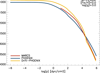
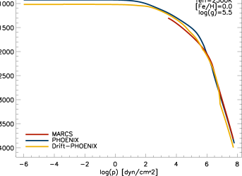
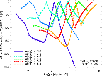
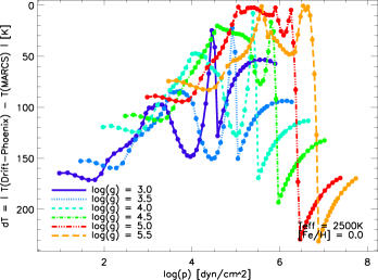
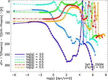
Figure 1: Top row: local gas temperature-pressure structures for T_eff = 2500K (log(g) = 3.0: top left; log(g) = 5.5: top right) for MARCS, Phoenix and Drift-Phoenix. Middle row: left - residual temperature values $dT_{\rm gas}$ between Phoenix and MARCS; right - $dT_{\rm gas}$ between Drift-Phoenix and MARCS. Bottom row: $dT_{\rm gas}$ between Drift-Phoenix and Phoenix model atmosphere results. Mixing length parameter: Phoenix - $l/H_{\rm p}$=2.79 for log(g) = 3.0 and $l/H_{\rm p}$=3.5 for log(g) = 5.5; MARCS - $l/H_{\rm p}$=1.5 for all models; Drift-Phoenix - $l/H_{\rm p}$=2.0 for all models.

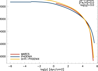
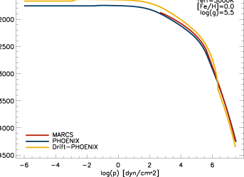
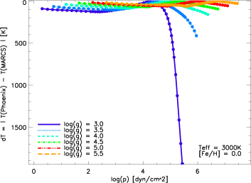
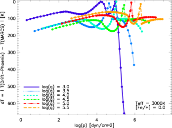
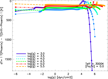
Figure 2: Top row: local gas temperature-pressure structures for T_eff = 3000K (log(g) = 3.0: top left; log(g) = 5.5: top right) for MARCS, Phoenix and Drift-Phoenix. Middle row: left - residual temperature values $dT_{\rm gas}$ between Phoenix and MARCS; right - $dT_{\rm gas}$ between Drift-Phoenix and MARCS. Bottom row: $dT_{\rm gas}$ between Drift-Phoenix and Phoenix model atmosphere results. Mixing length parameter: Phoenix - $l/H_{\rm p}$=2.3 for log(g) = 3.0 and $l/H_{\rm p}$=3.25 for log(g) = 5.5; MARCS - $l/H_{\rm p}$=1.5 for all models; Drift-Phoenix - $l/H_{\rm p}$=2.0 for all models.

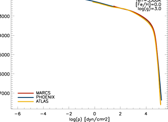
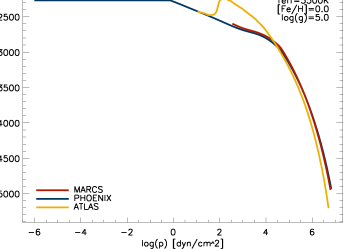
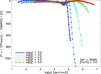
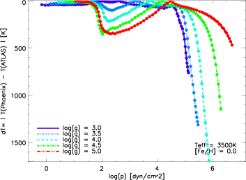
Figure 3: Top row: local gas temperature-pressure structures for T_eff = 3500K (log(g) = 3.0: top left; log(g) = 5.0: top right) for MARCS, Phoenix and ATLAS. Middle row: left - residual temperature values $dT_{\rm gas}$ between Phoenix and MARCS; right - $dT_{\rm gas}$ between ATLAS and MARCS. Bottom row: $dT_{\rm gas}$ between Phoenix and ATLAS model atmosphere results. Mixing length parameter: Phoenix - $l/H_{\rm p}$=1.99 for log(g) = 3.0 and $l/H_{\rm p}$=2.39 for log(g) = 5.0; ATLAS - $l/H_{\rm p}$=1.25 for all models; MARCS - $l/H_{\rm p}$=1.5 for all models.

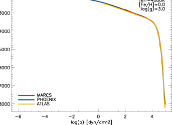
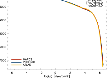
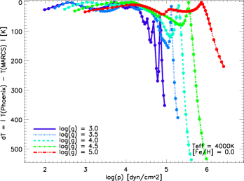
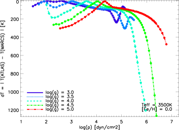
Figure 4: Top row: local gas temperature-pressure structures for T_eff = 4000K (log(g) = 3.0: top left; log(g) = 5.0: top right) for MARCS, Phoenix and ATLAS. Middle row: left - residual temperature values $dT_{\rm gas}$ between Phoenix and MARCS; right - $dT_{\rm gas}$ between ATLAS and MARCS. Bottom row: $dT_{\rm gas}$ between Phoenix and ATLAS model atmosphere results. Mixing length parameter: Phoenix - $l/H_{\rm p}$=1.82 for log(g) = 3.0 and $l/H_{\rm p}$=1.96 for log(g) = 5.0; ATLAS - $l/H_{\rm p}$=1.25 for all models; MARCS - $l/H_{\rm p}$=1.5 for all models.

Figures 1 – 4 present the comparison of the (T_gas, p_gas)-structures of MARCS, Phoenix, Drift-Phoenix and ATLAS for solar metallicity and T_eff = 2500, 3000, 3500 and 4000K, respectively. We observe better agreement between MARCS, Phoenix and Drift-Phoenix for T_eff = 2500K than for higher T_eff models. The 2500K sets of models do not vary by more than 300K (except for high pressure values). For all effective temperatures (T_eff=2500-4000K), the model atmospheres with higher surface gravity (brown dwarfs) agree better between different model families than those with lower surface gravity (giant gas planets, young brown dwarfs). Note these differences are hard to see in the top rows of Figs. 1 – 4 due to the scale of the plots. For this reason we provide plots of the calculated residuals in rows 2 and 3 of the figures.

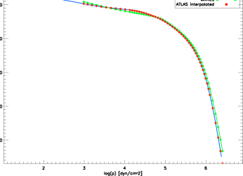
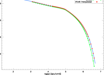
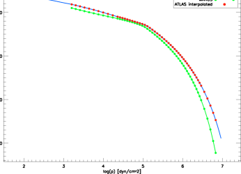
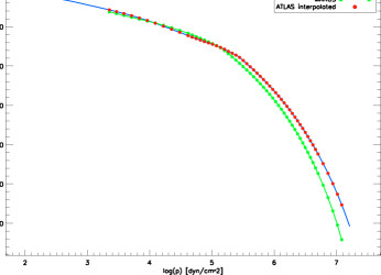
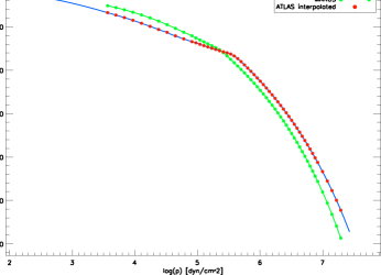
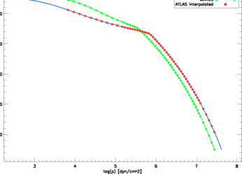
Figure 9: Local temperature-pressure structures of the ATLAS and MARCS models for T_eff = 4000K, log(g) = 5.0 and various metallicity values.

We compare the hot ATLAS and MARCS models for T_eff = 3500K and T_eff = 4000K. While the T_eff = 3500K models compare better in the low metallicity range -1.5 $<$ [M/H] $<$ -2.5, the T_eff = 4000K models display better agreement for higher metalicities [M/H] = +0.5 and [M/H] = 0.0. For both T_eff, the biggest discrepancies lie within the [M/H] = -1.0 models, with local gas temperature differences $dT_{\rm gas}>1500$K for the T_eff = 3500K and $dT_{\rm gas}>1200$K for the T_eff = 4000K case. All model families diverge with increasing local pressure, i.e. deeper in the atmosphere, regardless of T_eff, log(g) or metallicity [M/H]. The detailed plots for T_eff = 4000K, log(g) = 5.0 can be found in Appendix B, Figure 9.

In summary, we find that for the higher effective temperature values (3500K, 4000K) the ATLAS, Phoenix and MARCS (T_gas, p_gas)-structures diverge from each other with an average of $\sim$600K in local temperature and in extreme cases well over 1000K. The MARCS, Phoenix and Drift-Phoenix differ by an average of $\sim$300K for 2500K $<$ T_eff $<$ 4000K, with some extreme cases of over 1000K. Agreement improves as the surface gravity increases.

4 Comparing synthetic photometry

The (T_gas, p_gas)-structure determines the emergent spectral energy distribution for stars. In order to compare the SEDs of the different model atmosphere families, we perform synthetic photometry for all models considered. We convolve the model SEDs to the (UKIDSS) UKIRT WFCAM ZYHJK (Hewett et al., 2006), 2MASS JHKs (Cohen et al., 2003) and Johnson UBVRI (Johnson, 1965) filter systems, based on codes used in Sinclair et al. (2010). The wavelength ranges for these used filters are summarized in Table 6.

The convolved broad-band flux F_R is given by (Straizys, 1996)

$$F_{R}(\lambda)=\frac{\int_{\lambda_{1}}^{\lambda_{2}}F(\lambda)R(\lambda)d\lambda}{\int_{\lambda_{1}}^{\lambda_{2}}R(\lambda)d\lambda}$$ (1)

where R($\lambda$) is the throughput function (only filter transmission for the optical (UBVRI) bands, but filter transmission plus detector throughput for 2MASS/UKIDSS); and $\lambda_{\rm 1}$ and $\lambda_{\rm 2}$ are the limits of the filter wavelength range. Zero-point calibration is performed using the HST spectrum of Vega (Bohlin & Gilliland, 2004).

We proceed to calculate synthetic colour indices for each model atmosphere family. The colour indices are defines as

$$m_{1}-m_{2}=-2.5(\rm{log(\frac{F_{\rm R1}}{F_{\rm R1,Vega}})+log(\frac{F_{\rm R2}}{F_{\rm R2,Vega}})}).$$ (2)

A complete set of the synthetic photometry results is provided in Appendix C. In the following, we compare the ratios between the synthetic broad-band fluxes for all pairs of corresponding models in each filter. The closer the value to 1.0, the more similar the model atmosphere results are.

4.1 Optical bands (Johnson UBVRI filters)

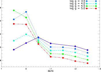
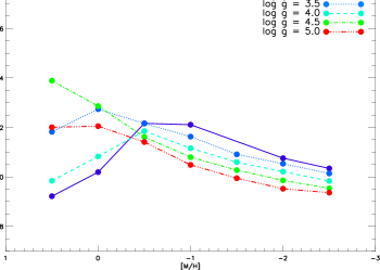
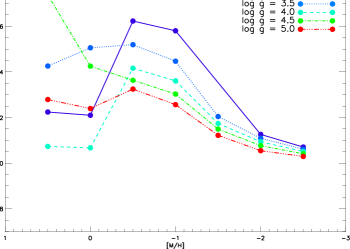
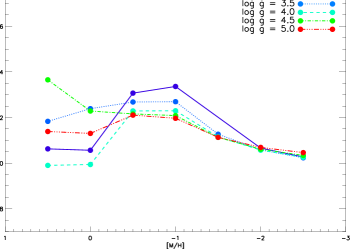
Figure 10: Synthetic flux ratios between for ATLAS/MARCS models in the optical Johnson UBVR bandpasses for T_eff = 3500 K

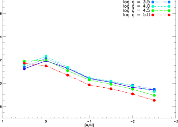
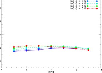
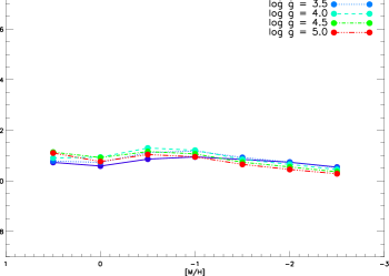
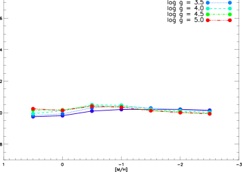
Figure 11: Synthetic flux ratios between for ATLAS/MARCS models in the optical Johnson UBVR bandpasses for T_eff = 4000 K

The broad-band fluxes of ATLAS and MARCS model atmospheres in the optical differ significantly more than those in the IR range. The flux ratios for T_eff = 3500K are deviating from 1.0 significantly more (as high as $\sim$1.8) than those for T_eff=4000K (less than $\sim$1.3). The ATLAS models predict more flux than MARCS in the U-band for metalicities above [M/H] = -1.0 and then drop to as low as about 20% less flux for [M/H] $>$ -1.0 for both effective temperatures. In the V-band, the ATLAS model predict systematically higher fluxes than MARCS. Corresponding plots are provided in Figures 10 and 11.

4.2 IR bands

Figures 5 and 6 represent the UKIDSS photometric flux ratios for Phoenix to MARCS and Phoenix to Drift-Phoenix. Phoenix and MARCS display a good agreement in the range T_eff = 3500$-$4000K. A possible explanation for the decreasing discrepancies in this T_eff range relative to T${}_{\rm eff}<$3000K is the lack of dust as effective temperature rises. Dust should not have an impact on the atmospheric structures in models with T${}_{\rm eff}>$3000K (Witte et al., 2009).

For decreasing effective temperature, the Phoenix models systematically predict more flux in the IR bands than the MARCS model atmospheres for higher log(g) values and less flux than MARCS for low log(g). The Y-band band is an exception to this trend, where, for T${}_{\rm eff}<$ 3500K all Phoenix models predict less flux than MARCS with the flux ratio dropping as low as 0.7. Both model families do not include cloud formation in the model atmospheres considered here, hence, the differences in fluxes may point to differences in the molecular opacities (line lists and/or gas-phase chemistry data).

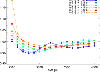
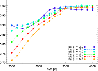
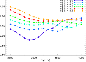
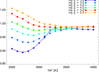
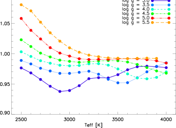
Figure 5: Convolved flux ratios for Phoenix and MARCS atmosphere models for the UKIDSS filter system. Curves are colour coded with respect to log(g) value: orange - 5.5, red - 5.0, green - 4.5, cyan - 4.0, blue - 3.5, dark blue - 3.0. All models here are of solar metallicity.

We compare the Phoenix and Drift-Phoenix model atmospheres (2500K $\leq$ T_eff $\leq$ 3000K) in order to check if the difference in dust treatment is sufficient to explain differences in synthetic fluxes (Fig. 6). Differences between these two families are generally smaller than in comparisons with the MARCS model atmospheres. For the H and J bands, all Phoenix atmosphere models predict less flux than Drift-Phoenix. This result is unexpected as these bands are heavily affected by dust and the Phoenix models are dust-free. Therefore, while still an important factor, the dust treatment alone cannot explain the observed trends in the comparison of the synthetic fluxes. All models produce very similar fluxes in the K band. For all bands, except in the Z band, the flux ratio is highest for the higher surface gravity values. This trend is reversed in the Z band, which also appears to vary the most with change in T_eff.

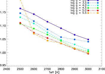
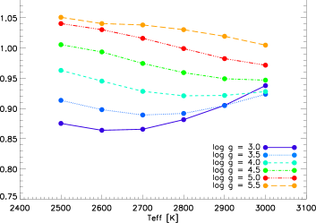
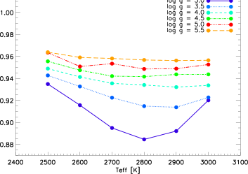
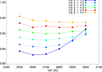
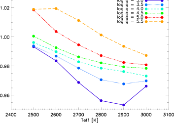
Figure 6: Convolved flux ratios for Phoenix and Drift-Phoenix atmosphere models for the UKIDSS filter system.

We also present the colour indices calculated for each model atmosphere family considered here (Figure 7 and Appendix C). All colours show considerable differences for model atmospheres T${}_{\rm eff}<3000$K. Dust starts to form in small amounts at T${}_{\rm eff}\approx 2700$K and the resulting element depletion of the gas-phase may contribute to the increasing differences with decreasing T_eff below 2700K (Witte et al., 2009). In particular, the B-V magnitudes differ by up to half a magnitude between the Drift-Phoenix and MARCS models in the low temperature half of the plot. The ATLAS models appear to differ significantly from all other model families considered here.

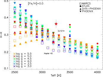
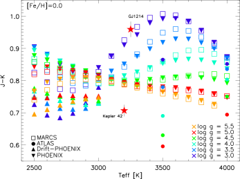
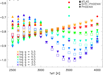
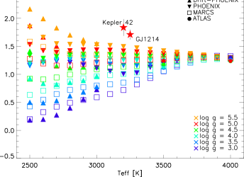
Figure 7: Colour indices versus effective temperature for all model atmosphere families (circles - ATLAS, squares - MARCS, lower triangles - Phoenix, upper triangles - Drift-Phoenix) of solar metallicity. The first three plots refer to the UKIDSS filter system. The two red stars are observed data for GJ 1214 and Kepler 42 (Anglada-Escude et al 2013; Muirhead et al. 2012; Cutri et al. 2003). The 2MASS measurements for these two stars have been shifted into the UKIDSS system using the transformations given in Hewett et al. 2006. Colour coding is used for different values for log(g) with a step of 0.5 dex. Top left: For lower T_eff, models with lower log(g) have higher H-K values than models with high log(g) . The trend inverses at higher temperatures. Top right: No clear trend with respect to log(g) is visible for lower T_eff. At higher temperatures models with lower log(g) show higher J-K values. Bottom left: No trend for lower T_eff. At higher temperatures models with higher log(g) have higher Z-J values. Bottom right: For low temperatures, models with high log(g) show a higher B-V value. The B-V difference with respect to log(g) diminishes for higher T_eff.

5 Discussion

5.1 Different model assumption

The differences in the atmospheric (T_gas, p_gas)-structures and the resulting SEDs arises from differences in input data (element abundances, opacity sources), physical assumptions (mixing length, overshooting, dust/ no dust), the choice of material values (equilibrium constants, line lists), but also from more technical details like convergence criteria and/or inner/outer boundary choices. It is outside the scope of this paper to identify in more detail why the model atmosphere results differ as this would require a dedicated benchmark study.

The ATLAS atmosphere models were developed for hotter stars and cover a wide range of metallicities, surface gravities and effective temperatures, from hot O and B down to early type M stars. The latest models use improved opacity distribution functions (ODFs) as described in Castelli & Kurucz (2004). The atomic and molecular line lists for the new ODFs are from the old Kurucz (1990) ODFs with some changes. A new TiO list from Schwenke (1998) is used. Additionally H₂O lines are adopted from Partridge & Schwenke (1997). Furthermore extra bands have been added for some molecules such as CN, OH and SiO. Linelest and ODFs can be found on Kurucz and Castelli’s webpages. Element abundances are solar and adopted from Grevesse & Sauval (1998). The models are calculated assuming mixing-length theory without overshooting, with a mixing length parameter l$/H_{\rm p}$ = 1.25 and line-broadening by a micro-turbulent velocity of v_turb = 2.0 km$/$s.

The MARCS models (Gustafsson et al., 2008) have focused on F, G and K stars extending into the M-dwarf regime. The opacity sampling method is used. Models are available for micro-turbulence velocities of v_turb = 0, 1, 2 and 5 km$/$s (for comparison purposes with ATLAS, we have only considered a value of 2 km$/$s). The mixing length parameter value is $1/H_{\rm p}$=1.5. The models are also divided in several metal abundance groups, out of which we consider the one with abundances from Grevesse et al. (2007). Molecular opacity sources include HCN, H₂O, C₂, C₃, C₂H₂, CH, CN, CaH, FeH, MgH, NH, OH, SiH, SiO, TiO, VO and ZrO. Continuous absorption sources are H I, H^-, H${}_{\rm 2}^{-}$, H${}_{\rm 2}^{+}$, He I, He^-, C I, C II, C^-, N I, N II, N^-, O I, O II, O^-, Mg I, Mg II, Al I, Al II, Si I, Si II, Ca I, Ca II, Fe I, Fe II, CH, OH, CO^- and H₂O^-. The codes also include collision-induces absorption from H I + H I, H I + He I, H₂ + H I, H₂ + H₂, H₂ + He I; continuous electron scattering and Rayleigh scattering for H I, H₂ and He I. The authors suggest that the only significant difference using different molecular opacity sources comes from CO, H₂O and TiO. CO sources adopted by (Gustafsson et al., 2008) (Table 2) are from Goorvitch (1994) and Kurucz (1995), H₂O from Barber et al. (2006) and TiO from Plez (1998).

The Phoenix models (Husser et al., 2013) are based on the Hauschildt & Baron (1999) stellar atmosphere code. The gas-phase chemistry is treated with the Astrophysical Chemical Equilibrium Solver (ACES, Witte et al. 2011). Husser et al. note that while condensation is included as element sink in the equation of state, it is omitted from opacity calculations and additionally no dust settlement is included in any of the models. The gas opacity species (line and continuum) are the same like in Drfit-Phoenix (see below). The code uses mixing length theory, with $1/H_{\rm p}\sim 1.8\ldots 3.5$ for the M-dwarf parameter space. The micro-turbulent velocity is linked to the convective velocity that results from mixing-lenth theory (MLT). However, the micro-turbulent velocity it is only considered in the calculations of the high-resolution spectra, but not used for the computation of the atmospheric structure. Based on this assumption, v${}_{\rm turb}<$ 1 km$/$s for Phoenix model atmospheres in the M-dwarf parameter range.

The Drift-Phoenix models are aimed at brown dwarf and planet atmospheres. They are a combination of the Phoenix atmosphere code (Hauschildt & Baron, 1999), version 16.00.02A, and the Drift module (Witte et al. 2009, Helling, Woitke & Thi 2008) that models cloud formation. Drift solves a system of element conservation and dust moment equations in phase non-equilibrium including the processes of dust nucleation, growth and/or evaporation. The influence of gravitational settling and element replenishment by convective overshooting is considered in relation to the formation processes. Six main elements are considered in these processes - Ti, O, Al, Fe, Si and Mg, together with the seven most important solids consisting of these elements - TiO₂[s], Al₂O₃[s], Fe[s], SiO₂[s], MgO[s], MgSiO₃[s] and Mg₂SiO₄[s]. The line opacity sources considered include H₂, CH, NH, OH, MgH, SiH, CN, SiO, CO₂, O₃, N${}_{\rm 2}^{\rm-}$O, CH₄, SO₂, NH₃, HCl, N₂, VO, CaH, CrH and FeH. Collision induced absorption sources include H₂ - H₂, H₂ - He, H₂ - CH₄, H₂ - N₂, N₂ - CH₄, N₂ - N₂, CH₄ - CH₄, CO₂ - CO₂, Ar - H₂ and Ar - CH₄. CO lines are adopted from Goorvitch (1994), H₂O from Barber & Tennyson (2008) and TiO from Schwenke (1998). Mie and effective medium theory are applied to calculate the cloud opacity of mixed grains including the above mentioned solid materials.

Only the Phoenix and Drift-Phoenix model families use the same line lists for gas opacity sources, and only MARCS and Drift-Phoenix use the same values for the element abundances (Grevesse et al., 2007). It is therefore not surprising that the model fluxes differ particular for low T_eff, where the influence of molecular and dust opacity is most prominent. In addition, there are differences in input parameter values such as the mixing length parameter. Husser et al. 2013 (their Sect. 2.3.3) suggest that the micro-turbulent velocities does have no noticeable effect on the atmospheric structure computation results.

We further note that (Gustafsson et al., 2008) presented a comparison of the Marcs model atmospheres to ATLAS and Phoenix (NextGen) model atmospheres as available at the time. Their comparison of the ($T_{\rm gas}$, $p_{\rm gas}$)-structures of Marcs andATLAS model atmospheres for giants and supergiants for log(g)=4.5 and T${}_{\rm eff}=4000,5000,6000,7000$K did show a respectiable agreement between the models. The same holds for their test of varying metalicities, and for a comparison to NextGen Phoenix models with (log(g), T_eff)= (0.0, 3000K), (3.0, 5000K). No radiation fluxes were compared. Plez (2011) presented comparison of synthetic Johnson-Cousins UBVRIJHK photometry and colours of Marcs, ATLAS and Phoenix (NextGen) model atmospheres for T${}_{\rm eff}=3500\,\ldots\,8000$K. Plez (2011) demonstrate that differences do increase with decreasing T_eff particulare for T${}_{\rm eff}<4000$K. Our study presented in this paper does support these findings and extend these early model comparisons into the M-dwarf regime.

5.2 Comparing synthetic photometry and observations

We compare the synthetic photometry for all three model atmosphere families with two observations:

• We compare the synthetic photometry results with observations for the M stars published in Koen et al. (2010)

• The B-V, J-K and H-K colours of two observed M-dwarf planet host stars (Kepler 42, Muirhead et al. 2012; GJ1214, Anglada-Escude et al 2013) are included in Fig. 7 for comparison.

All objects of spectral type M, and for which optical and infrared photometry was available, were selected from Tables 2 & 4 Koen et al. (2010) for our comparison. The majority of this sample of objects are early M stars with T${}_{\rm eff}\approx$4000K and log(g)$\approx$4.5. Table 13 lists the names, associated photometric magnitudes and spectral types of all stars used for this comparison. Only the MARCS and the Phoenix model families cover the respective parameter range. Figure 8 presents a colour plot of the photometry that compares the MARCS and Phoenix model results with the sample of observed M stars.

Early M dwarfs are represented by model atmospheres with T${}_{\rm eff}\approx 4000$K, and the sample of observed M dwarfs does not contain examples with T${}_{\rm eff}<3500$K. Therefore, the upper half of the plot is empty, hence, it does not imply the models are giving incorrect predictions for these effective temperatures. The spectral type of the observed targets explains the lack of objects in the upper half of the plots and is not a mismatch between models and observations. For log(g)$=4.5$ the median of the observed colours is well reproduced by the atmosphere models. For higher log(g), the observed colours are redder than predicted by atmosphere models. However, the scatter in the observations is larger than the differences in the models would suggest. The measurement uncertainties $\sim$ 0.01 mag (Koen et al. (2010)) are not big enough to account for the scatter in the observed data.

The reason for the differences between models and observations is not obvious. One reason could be a mismatch between the metallicities of the stars and the (solar) metallicity in the models. Note that not all objects in Fig. 8 have reliably measured metallicities, hence, the scatter of the observed data could be partly due to varying stellar metallicities. The comparison between the exoplanet host stars strengthens this hypothesis. While GJ1214 has approximately solar metallicity, Kepler-42 is reported to have sub-solar metallicity ( [Fe/H]$=-0.48\pm 0.17$ and [M/H]$=-0.33\pm 0.12$, Muirhead et al. 2012). GJ1214 is significantly redder in near-infrared colours than Kepler-42, but still only marginally consistent with the H-K colour predicted from atmosphere models. Both objects are redder in B-V than all predictions from the models.

Alternatively, the mismatch could be caused by physical processes not included in the models considered here, for example, effects related to the presence of strong magnetic fields (e.g. Vidotto et al. 2013). It has been shown that strong magnetic fields can alter the fundamental properties of cool stars, in particular, suppress the temperature and inflate the radius. A temperature suppression of up to 200-400 K is realistic for early M-type stars, see Stassun et al. 2012). This could possibly explain an increase of up to 0.1 mag in the J-K colour (see Figs. 7). In summary, the best explanation for the scatter in the observed datapoints in Fig. 8 is probably a combination of a range of metallicities and the presence of magnetic fields, whereas the contribution from measurement uncertainties is only minor.

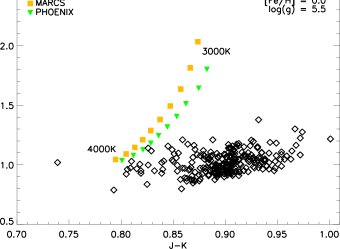
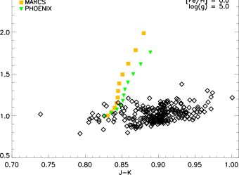
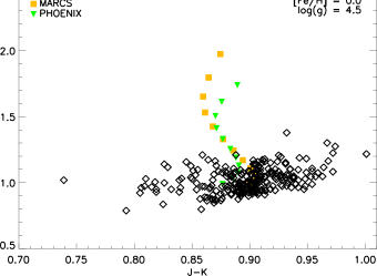
Figure 8: Colour-colour plot for a set of observed M stars (black diamonds, 13) and synthetic photometry of MARCS (yellow sqaures) and Phoenix (green triangles) models for T_eff = 3000 - 4000K, [M/H] = 0.0 and log(g) = 5.5 - 4.5. Each panel contains sets of models for a particular value of log(g). The model T_eff changes from 3000K for higher y-axis values to 4000K for lower y-axis values in each panel. Observed sample is adopted from the UBVRI, JHK photometry of Koen et al. (2010). It contains stars with various temperatures, surface gravity and metalicity values. The entire sample is plotted in all three panels. Typical observational uncertainty for the sample is $\sim$0.01mag for both, optical and ifrared. The median of the observed colours is well reproduced by the log(g) = 4.5 atmosphere models. Scatter in the observations is larger than the differences in the models would suggest.

5.3 Implications of host-star’s uncertainties for exoplanets

Estimating exoplanetary mass and radius directly depends on knowledge of the host star’s mass and radius. Most often, they are derived by comparison to evolutionary models which, however, already carry the uncertainties in model atmospheres discussed in the previous sections. Stellar atmosphere models can provide values for surface gravity, log(g), but there is still a degeneracy in possible values for stellar mass and radius.

An important property for a star-planet(s) system is the habitable zone (HZ). The habitable zone refers to the distance away from the star where liquid water could exist on the surface of a planet, provided sufficient atmospheric pressure. Detailed calculations for the extent of the HZ have been conducted by Kasting et al. (1993), Jones & Sleep (2010) and Kopparapu et al. (2013). Kane (2014) uses their methods to estimate the uncertainty of the habitable zones location (resulting from stellar parameter (effective temperature, radius, surface gravity, mass) uncertainties) for confirmed exoplanetary host stars and Kepler candidate hosts. The author demonstrates that $\sim$ 5% uncertainties in T_eff result in $\sim$ 10% uncertainty in the HZ location. Furthermore, the HZ distance is shown to have a linear dependence on the stellar radius R_∗ and hence proportional to $\sqrt{1/\rm{g}}$ and $\sqrt{\rm{M_{*}}}$, where g and M_∗ are the stellar surface gravity and mass. The system Kepler-27 is used as an example where the host star’s parameters have large uncertainties. The associated error in the HZ region is demonstrated to be large enough, so that a planet in habitable zone may very well lie outside of it on a 1-$\sigma$ level. The author further states that this is the case for the majority of Kepler candidates.

Plavchan et al. (2014) compare transit durations of Kepler targets to a synthetic distribution crated based on eccentricities of exoplanets discovered by the radial velocity method. The authors find an over-abundance of Kepler targets with transit durations longer than expected and a median transit duration of $\sim$25% longer than predicted. These effects are both attributed to under-estimates of the stellar radii. In addition, a statistically significant trend is found in the average transit duration as a function of stellar mass and radius which is explained by errors in determination of stellar radii as a function of spectral type.

A particularly underestmated factor for M-dwarfs is their strong magnetic field activity. The magnetic activity of the host star can have strong implications for the habitability of a planet. Vidotto et al. (2013), Vidotto et al. (2014) address planetary magnetoshpere size in relation to the stellar magnetic fields and show that for non-axisymmetric stellar magnetic field topologies, the size of the planetary magnetosphere can expand/shrink by up to 20% along its orbit. In addition the authors argue that planets in systems around host stars with such magnetic field topologies will be better shielded against galactic cosmic rays even in the absence of a thick planetary atmosphere or a large planetary magnetosphere.

6 Summary

We compared ATLAS9, MARCS, Phoenix and Drift-Phoenix atmosphere models in the M-dwarf parameter range that includes young M-dwarfs and also brown dwarfs. Our study has been inspired by the first model atmosphere comparsion in Gustafsson et al. (2008) and in Plez (2011) which focused on T${}_{\rm eff}>3500$K, and by extensive studies for space missions as in Sarro et al. (2013). Our comparison of (T_gas, p_gas) structures for T${}_{\rm eff}<3500$K reveals difference in local temperatures between the MARCS, Phoenix, and Drift-Phoenix model atmosphere families of, on average, less than 300K. Such a variation becomes significant for low T_eff models, where dust condensation plays a major role for the shape of the SED.

We compiled UKIDSS ZYJHK, 2MASS JHKs and Johnson UBVRI synthetic photometric data for the ATLAS, MARCS, Phoenix, and Drift-Phoenix model families. Colour indices differ between models by no more than 0.15 dex in the IR range. Both, atmospheric structure and synthetic photometry data, suggests that model atmospheres with higher surface gravity agree better between different models regardless of their T_eff. Comparing to observational data, the difference in the models is smaller than the typical observational errors of 0.01 mag. However a spread in the data is present which is not account for by the models, which may suggest a mismatch between model and stellar metallicities.

The present paper demonstrated differences and similarities between various model atmosphere families which allows a better estimate of systematic uncertainty values that may result from our limitted capacity of modelling every aspect of atmosphere physics and chemistry in the best possible way, and from the tentativeness of the ’best possible way’. Optimally, more than one model family should be used when working with observational data. The need for model atmosphere diversity has been demonstrated, for example, with respect to disk detection (Sinclair et al., 2010) or determining planetary parameter (Southworth, 2012). Such studies suggest that a similar multi-model approach could be beneficial for studies as for example performed in Sarro et al. (2013) who present a module that will be used to detect and characterise ultra-cool dwarfs in the Gaia database.

7 Acknowledgments

We thank the authors of the ATLAS9, MARCS, Phoenix and Drift-Phoenix model atmosphere grids to allow us to use their model results for this comparison study, and for their helpful suggestions. We thank Dr Tim-Oliver Husser (Institut für Astrophysik, Georg-August-Universitat Göttingen) for his support with the Phoenix models. We also thank Sören Witte and our referee for constructive feedback. ChH highlights financial support of the European Community under the FP7 by an ERC starting grant. IB thanks the Physics Trust of the University of St Andrews for supporting her summer placement. Most literature search was performed using the ADS. Our local computer support is highly acknowledged.

Appendix A Parameter values of models used

Tables A1 - A4 indicate availability of models of different families for various parameter value combinations.

The tables below describe the parameter values for all the models used in this work. Empty cells indicate that a given set of parameter values was not used as the corresponding model was missing in some model family.

Table 2: Common models between ATLAS and MARCS for T_eff = 3500K

	-2.5	-2.0	-1.5	-1.0	-0.5	0.0	+0.5
3.0	X	X		X	X	X	X
3.5	X	X	X	X	X	X	X
4.0	X	X	X	X	X	X	X
4.5	X	X	X	X	X	X	X
5.0	X	X	X	X	X	X	X

Table 3: Common models between ATLAS and MARCS for T_eff = 4000K

	-2.5	-2.0	-1.5	-1.0	-0.5	0.0	+0.5
3.0	X	X	X	X	X	X	X
3.5	X	X	X	X	X	X	X
4.0	X	X	X	X	X	X	X
4.5	X	X	X	X	X	X	X
5.0	X	X	X	X	X	X	X

Table 4: Common models between MARCS, Phoenix and Drift-Phoenix for [M/H] = 0.0

	2500	2600	2700	2700	2800	2900	3000
3.0	X	X	X	X	X	X	X
3.5	X	X	X	X	X	X	X
4.0	X	X	X	X	X	X	X
4.5	X	X	X	X	X	X	X
5.0	X	X	X	X	X	X	X
5.5	X	X	X	X	X	X	X

Table 5: Additional common models between MARCS, Phoenix for [M/H] = 0.0

	3100	3200	3300	3400	3500	3600	3700	3800	3900	4000
3.0	X	X	X	X	X	X	X	X	X	X
3.5	X	X	X	X	X	X	X	X	X	X
4.0	X	X	X	X	X	X	X	X	X	X
4.5	X	X	X	X	X	X	X	X	X	X
5.0	X	X	X	X	X	X	X	X	X	X
5.5	X	X	X	X	X	X	X	X	X	X

Appendix B Complementary T-p structure and flux ration plots

Figure B1 presents a sample of plots illustrating the difference in temperature-pressure structures between ATLAS and MARCS models in the metallicity parameter space. Figure B2 gives synthetic flux ratios in the optical bands fro the ATLAS and MARCS models.

Appendix C Synthetic flux and colour data

Table 6 summarises the filter wavelength ranges where throughput values are above 1% for the systems used in this study. 7-12 provide a complete set of synthetic fluxes for all models discussed in this work. Table 13 contains photometric data for the sample M-dwarfs used for the comparison with synthetic colours in Section 5.2.

Table 6: Wavelength range for filters used for synthetic photometry. The range is given for throughput values above 1%

Filter	Wavelength range
UKIDSS Z	0.82$-$0.94 $\mu$m
UKIDSS Y	0.96$-$1.10 $\mu$m
UKIDSS J	1.15$-$1.35 $\mu$m
UKIDSS H	1.45$-$1.82 $\mu$m
UKIDSS K	1.96$-$2.44 $\mu$m
2MASS J	1.08$-$1.41 $\mu$m
2MASS H	1.48$-$1.82 $\mu$m
2MASS Ks	1.95$-$2.36 $\mu$m
Johnson U	3050$-$4100 $\AA$
Johnson B	3700$-$5500 $\AA$
Johnson V	4700$-$7300 $\AA$
Johnson R	5250$-$9450 $\AA$
Johnson I	6900$-$11800 $\AA$

Table 7: Complete set of Phoenix synthetic fluxes for models of solar metalicity. The values in the filter columns correspond to $-2.5\rm{log({F_{\rm R1}}/{F_{\rm R1,Vega}}})$, where R1 is the corresponding filter. Column 3-7 refer to the Johnson and columns 11-15 to the UKIDSS filters.

Teff	log(g)	U	B	V	R	I	2MASS H	2MASS J	2MASS Ks	H	J	K	Y	Z
2500	3.0	11.50	10.99	9.83	7.32	5.05	2.51	3.10	2.12	2.57	2.97	2.07	2.97	2.07
2500	3.5	11.74	11.03	9.88	7.32	5.02	2.47	3.08	2.10	2.53	2.95	2.05	2.95	2.05
2500	4.0	12.14	11.14	9.95	7.32	5.01	2.43	3.05	2.08	2.49	2.93	2.03	2.93	2.03
2500	4.5	12.72	11.33	9.99	7.30	5.00	2.39	3.03	2.07	2.45	2.90	2.02	2.90	2.02
2500	5.0	13.46	11.52	9.99	7.24	4.96	2.34	3.00	2.06	2.40	2.87	2.03	2.87	2.03
2500	5.5	14.43	11.63	9.79	7.03	4.83	2.33	2.98	2.11	2.38	2.85	2.08	2.85	2.08
2600	3.0	10.97	10.44	9.23	6.89	4.77	2.37	2.96	2.00	2.43	2.83	1.96	2.83	1.96
2600	3.5	11.15	10.44	9.23	6.87	4.74	2.34	2.94	1.98	2.40	2.82	1.94	2.82	1.94
2600	4.0	11.46	10.52	9.29	6.87	4.72	2.30	2.92	1.96	2.36	2.80	1.92	2.80	1.92
2600	4.5	11.94	10.68	9.40	6.89	4.71	2.26	2.89	1.95	2.32	2.77	1.91	2.77	1.91
2600	5.0	12.59	10.91	9.48	6.89	4.70	2.22	2.87	1.94	2.27	2.75	1.90	2.75	1.90
2600	5.5	13.43	11.14	9.48	6.84	4.66	2.19	2.85	1.96	2.24	2.72	1.93	2.72	1.93
2700	3.0	10.50	9.96	8.73	6.53	4.53	2.24	2.82	1.89	2.29	2.70	1.85	2.70	1.85
2700	3.5	10.62	9.89	8.65	6.46	4.48	2.21	2.81	1.87	2.26	2.69	1.83	2.69	1.83
2700	4.0	10.86	9.94	8.67	6.45	4.45	2.18	2.79	1.86	2.23	2.67	1.81	2.67	1.81
2700	4.5	11.25	10.07	8.75	6.47	4.44	2.14	2.77	1.84	2.19	2.65	1.80	2.65	1.80
2700	5.0	11.79	10.26	8.87	6.50	4.43	2.10	2.74	1.83	2.15	2.62	1.79	2.62	1.79
2700	5.5	12.53	10.52	8.97	6.51	4.41	2.07	2.72	1.83	2.12	2.60	1.80	2.60	1.80
2800	3.0	10.06	9.51	8.30	6.22	4.30	2.08	2.68	1.77	2.13	2.56	1.73	2.56	1.73
2800	3.5	10.12	9.39	8.13	6.10	4.24	2.08	2.68	1.76	2.13	2.56	1.72	2.56	1.72
2800	4.0	10.31	9.39	8.10	6.06	4.20	2.06	2.67	1.75	2.11	2.55	1.71	2.55	1.71
2800	4.5	10.62	9.48	8.14	6.07	4.19	2.03	2.65	1.73	2.08	2.54	1.70	2.54	1.70
2800	5.0	11.08	9.65	8.23	6.09	4.18	1.99	2.63	1.72	2.04	2.52	1.69	2.52	1.69
2800	5.5	11.71	9.87	8.34	6.12	4.16	1.95	2.61	1.72	2.00	2.49	1.69	2.49	1.69
2900	3.0	9.68	9.10	7.94	5.94	4.09	1.92	2.54	1.64	1.96	2.42	1.60	2.42	1.60
2900	3.5	9.68	8.94	7.69	5.78	4.01	1.94	2.54	1.65	1.99	2.43	1.61	2.43	1.61
2900	4.0	9.81	8.90	7.60	5.72	3.98	1.94	2.54	1.64	1.98	2.43	1.60	2.43	1.60
2900	4.5	10.06	8.95	7.59	5.70	3.96	1.92	2.54	1.63	1.96	2.43	1.60	2.43	1.60
2900	5.0	10.44	9.07	7.64	5.71	3.94	1.88	2.52	1.62	1.93	2.41	1.59	2.41	1.59
2900	5.5	10.96	9.27	7.73	5.74	3.93	1.85	2.50	1.61	1.89	2.39	1.58	2.39	1.58
3000	3.0	9.33	8.72	7.61	5.69	3.90	1.73	2.41	1.49	1.78	2.30	1.46	2.30	1.46
3000	3.5	9.27	8.52	7.30	5.50	3.81	1.79	2.41	1.52	1.83	2.30	1.49	2.30	1.49
3000	4.0	9.35	8.45	7.15	5.40	3.76	1.81	2.42	1.53	1.85	2.31	1.50	2.31	1.50
3000	4.5	9.54	8.46	7.10	5.37	3.74	1.80	2.42	1.53	1.84	2.31	1.50	2.31	1.50
3000	5.0	9.85	8.55	7.12	5.36	3.73	1.78	2.41	1.52	1.82	2.30	1.49	2.30	1.49
3000	5.5	10.30	8.71	7.18	5.38	3.72	1.75	2.40	1.51	1.79	2.29	1.48	2.29	1.48
3100	3.0	9.02	8.35	7.30	5.46	3.71	1.54	2.29	1.33	1.59	2.18	1.30	2.18	1.30
3100	3.5	8.92	8.13	6.95	5.24	3.61	1.63	2.29	1.39	1.67	2.19	1.36	2.19	1.36
3100	4.0	8.94	8.04	6.76	5.12	3.57	1.67	2.30	1.42	1.71	2.20	1.39	2.20	1.39
3100	4.5	9.08	8.03	6.68	5.06	3.55	1.69	2.31	1.43	1.73	2.20	1.40	2.20	1.40
3100	5.0	9.33	8.09	6.66	5.04	3.53	1.68	2.30	1.43	1.72	2.20	1.40	2.20	1.40
3100	5.5	9.69	8.20	6.69	5.05	3.52	1.65	2.30	1.42	1.69	2.19	1.39	2.19	1.39
3200	3.0	8.73	8.00	7.00	5.23	3.54	1.36	2.17	1.18	1.41	2.06	1.15	2.06	1.15
3200	3.5	8.60	7.77	6.62	5.00	3.44	1.47	2.18	1.25	1.52	2.08	1.23	2.08	1.23
3200	4.0	8.58	7.66	6.40	4.86	3.39	1.54	2.19	1.30	1.58	2.09	1.27	2.09	1.27
3200	4.5	8.67	7.63	6.29	4.79	3.36	1.57	2.20	1.33	1.61	2.09	1.30	2.09	1.30
3200	5.0	8.86	7.66	6.25	4.75	3.35	1.57	2.20	1.33	1.61	2.10	1.30	2.10	1.30
3200	5.5	9.15	7.75	6.25	4.74	3.34	1.56	2.19	1.33	1.60	2.09	1.30	2.09	1.30
3300	3.0	8.51	7.68	6.66	5.00	3.39	1.22	2.08	1.05	1.27	1.97	1.03	1.97	1.03
3300	3.5	8.34	7.45	6.30	4.77	3.28	1.33	2.08	1.13	1.37	1.98	1.10	1.98	1.10
3300	4.0	8.27	7.32	6.07	4.62	3.22	1.41	2.09	1.19	1.45	1.99	1.16	1.99	1.16
3300	4.5	8.30	7.27	5.94	4.53	3.19	1.45	2.10	1.22	1.49	1.99	1.20	1.99	1.20
3300	5.0	8.44	7.28	5.88	4.48	3.18	1.47	2.10	1.24	1.51	2.00	1.21	2.00	1.21
3300	5.5	8.67	7.34	5.87	4.46	3.17	1.47	2.10	1.24	1.50	2.00	1.22	2.00	1.22
3400	3.0	8.34	7.34	6.22	4.70	3.23	1.11	2.01	0.94	1.16	1.91	0.93	1.91	0.93
3400	3.5	8.12	7.15	5.97	4.53	3.14	1.21	1.99	1.01	1.25	1.89	0.99	1.89	0.99
3400	4.0	8.00	7.01	5.75	4.38	3.07	1.29	1.99	1.08	1.33	1.89	1.05	1.89	1.05
3400	4.5	7.99	6.94	5.62	4.29	3.04	1.34	2.00	1.12	1.38	1.90	1.10	1.90	1.10
3400	5.0	8.07	6.93	5.55	4.24	3.02	1.37	2.00	1.15	1.40	1.90	1.12	1.90	1.12
3400	5.5	8.24	6.97	5.53	4.21	3.01	1.38	2.00	1.16	1.41	1.91	1.13	1.91	1.13

Table 8: continued

Teff	log(g)	U	B	V	R	I	2MASS H	2MASS J	2MASS Ks	H	J	K	Y	Z
3500	3.0	8.14	6.99	5.81	4.42	3.07	1.01	1.93	0.84	1.05	1.83	0.83	1.83	0.83
3500	3.5	7.92	6.84	5.61	4.28	3.00	1.09	1.91	0.91	1.13	1.81	0.90	1.81	0.90
3500	4.0	7.76	6.71	5.43	4.14	2.93	1.18	1.91	0.98	1.22	1.81	0.96	1.81	0.96
3500	4.5	7.71	6.64	5.31	4.06	2.90	1.24	1.91	1.03	1.27	1.81	1.00	1.81	1.00
3500	5.0	7.73	6.62	5.25	4.01	2.88	1.27	1.91	1.06	1.31	1.81	1.03	1.81	1.03
3500	5.5	7.85	6.64	5.22	3.98	2.87	1.29	1.91	1.08	1.32	1.82	1.05	1.82	1.05
3600	3.0	7.93	6.63	5.39	4.12	2.93	0.92	1.85	0.76	0.96	1.75	0.75	1.75	0.75
3600	3.5	7.72	6.53	5.27	4.03	2.86	0.99	1.84	0.82	1.03	1.74	0.81	1.74	0.81
3600	4.0	7.54	6.42	5.13	3.92	2.80	1.07	1.83	0.88	1.11	1.73	0.87	1.73	0.87
3600	4.5	7.45	6.35	5.02	3.84	2.77	1.14	1.82	0.94	1.17	1.73	0.92	1.73	0.92
3600	5.0	7.44	6.32	4.97	3.79	2.74	1.18	1.82	0.97	1.21	1.73	0.95	1.73	0.95
3600	5.5	7.51	6.34	4.95	3.77	2.73	1.20	1.82	1.00	1.23	1.73	0.97	1.73	0.97
3700	3.0	7.69	6.28	5.00	3.84	2.78	0.85	1.77	0.69	0.89	1.67	0.69	1.67	0.69
3700	3.5	7.50	6.23	4.94	3.79	2.73	0.89	1.75	0.74	0.93	1.66	0.73	1.66	0.73
3700	4.0	7.33	6.15	4.84	3.70	2.68	0.97	1.75	0.80	1.01	1.65	0.78	1.65	0.78
3700	4.5	7.21	6.08	4.76	3.63	2.64	1.04	1.74	0.85	1.08	1.65	0.84	1.65	0.84
3700	5.0	7.16	6.05	4.71	3.58	2.62	1.09	1.74	0.89	1.12	1.64	0.87	1.64	0.87
3700	5.5	7.19	6.05	4.69	3.56	2.60	1.12	1.74	0.92	1.15	1.64	0.90	1.64	0.90
3800	3.0	7.42	5.96	4.66	3.58	2.65	0.79	1.69	0.64	0.83	1.60	0.64	1.60	0.64
3800	3.5	7.26	5.93	4.64	3.56	2.61	0.81	1.67	0.66	0.85	1.58	0.66	1.58	0.66
3800	4.0	7.11	5.88	4.58	3.50	2.57	0.87	1.66	0.72	0.91	1.57	0.71	1.57	0.71
3800	4.5	6.98	5.82	4.51	3.43	2.53	0.95	1.66	0.77	0.98	1.57	0.76	1.57	0.76
3800	5.0	6.90	5.79	4.46	3.39	2.50	1.01	1.66	0.81	1.04	1.56	0.80	1.56	0.80
3800	5.5	6.90	5.79	4.45	3.37	2.48	1.04	1.66	0.84	1.07	1.56	0.82	1.56	0.82
3900	3.0	7.12	5.64	4.35	3.34	2.52	0.74	1.61	0.60	0.77	1.52	0.60	1.52	0.60
3900	3.5	7.01	5.64	4.36	3.33	2.49	0.74	1.60	0.60	0.78	1.50	0.60	1.50	0.60
3900	4.0	6.88	5.62	4.33	3.30	2.45	0.79	1.59	0.64	0.82	1.49	0.64	1.49	0.64
3900	4.5	6.75	5.58	4.28	3.25	2.42	0.86	1.58	0.70	0.89	1.49	0.68	1.49	0.68
3900	5.0	6.65	5.55	4.24	3.21	2.39	0.92	1.58	0.74	0.95	1.48	0.73	1.48	0.73
3900	5.5	6.62	5.54	4.22	3.19	2.37	0.96	1.57	0.77	0.99	1.48	0.76	1.48	0.76
4000	3.0	6.82	5.37	4.09	3.13	2.39	0.69	1.53	0.56	0.73	1.44	0.56	1.44	0.56
4000	3.5	6.72	5.36	4.10	3.13	2.37	0.68	1.52	0.56	0.72	1.42	0.55	1.42	0.55
4000	4.0	6.62	5.35	4.10	3.11	2.34	0.71	1.51	0.58	0.74	1.41	0.57	1.41	0.57
4000	4.5	6.51	5.34	4.07	3.08	2.31	0.77	1.50	0.62	0.80	1.41	0.62	1.41	0.62
4000	5.0	6.41	5.31	4.03	3.04	2.28	0.83	1.50	0.67	0.86	1.40	0.66	1.40	0.66

Table 9: Complete set of MARCS synthetic fluxes for models of solar metalicity. The values in the filter columns correspond to $-2.5\rm{log({F_{\rm R1}}/{F_{\rm R1,Vega}}})$, where R1 is the corresponding filter. Column 3-7 refer to the Johnson and columns 11-15 to the UKIDSS filters.

Teff	log(g)	U	B	V	R	I	2MASS H	2MASS J	2MASS Ks	H	J	K	Y	Z
2500	3.0	11.19	11.16	10.96	7.61	5.03	2.43	3.00	2.09	2.49	2.87	2.04	2.87	2.04
2500	3.5	11.64	11.32	10.90	7.57	5.02	2.42	3.03	2.08	2.49	2.89	2.04	2.89	2.04
2500	4.0	12.26	11.60	10.97	7.59	5.02	2.41	3.03	2.08	2.47	2.90	2.04	2.90	2.04
2500	4.5	13.14	12.00	11.08	7.64	5.03	2.39	3.04	2.09	2.45	2.91	2.05	2.91	2.05
2500	5.0	14.30	12.43	11.16	7.70	5.02	2.38	3.04	2.13	2.44	2.91	2.09	2.91	2.09
2500	5.5	15.53	12.78	11.20	7.77	4.99	2.38	3.04	2.20	2.43	2.91	2.17	2.91	2.17
2600	3.0	10.66	10.55	10.23	7.16	4.74	2.28	2.85	1.97	2.34	2.72	1.92	2.72	1.92
2600	3.5	11.02	10.65	10.11	7.10	4.72	2.28	2.88	1.96	2.34	2.75	1.92	2.75	1.92
2600	4.0	11.51	10.85	10.14	7.10	4.71	2.27	2.89	1.96	2.33	2.76	1.91	2.76	1.91
2600	4.5	12.21	11.16	10.25	7.14	4.72	2.25	2.89	1.96	2.31	2.77	1.92	2.77	1.92
2600	5.0	13.18	11.54	10.35	7.20	4.71	2.24	2.90	1.98	2.29	2.77	1.94	2.77	1.94
2600	5.5	14.32	11.90	10.41	7.26	4.70	2.23	2.90	2.04	2.29	2.77	2.00	2.77	2.00
2700	3.0	10.20	10.02	9.60	6.77	4.47	2.12	2.70	1.84	2.18	2.57	1.80	2.57	1.80
2700	3.5	10.47	10.04	9.39	6.67	4.44	2.15	2.74	1.85	2.20	2.61	1.80	2.61	1.80
2700	4.0	10.85	10.17	9.37	6.65	4.43	2.14	2.75	1.84	2.19	2.63	1.80	2.63	1.80
2700	4.5	11.40	10.40	9.45	6.68	4.43	2.12	2.76	1.84	2.18	2.64	1.80	2.64	1.80
2700	5.0	12.20	10.72	9.56	6.73	4.43	2.11	2.76	1.85	2.16	2.64	1.81	2.64	1.81
2700	5.5	13.20	11.06	9.65	6.79	4.42	2.10	2.76	1.89	2.15	2.64	1.85	2.64	1.85
2800	3.0	9.81	9.56	9.07	6.43	4.24	1.95	2.56	1.71	2.00	2.44	1.67	2.44	1.67
2800	3.5	9.99	9.49	8.77	6.29	4.19	2.00	2.60	1.73	2.06	2.48	1.69	2.48	1.69
2800	4.0	10.28	9.55	8.68	6.24	4.17	2.01	2.62	1.73	2.06	2.51	1.69	2.51	1.69
2800	4.5	10.71	9.72	8.72	6.25	4.16	2.00	2.63	1.73	2.05	2.52	1.69	2.52	1.69
2800	5.0	11.34	9.97	8.81	6.29	4.16	1.98	2.63	1.73	2.03	2.52	1.70	2.52	1.70
2800	5.5	12.19	10.28	8.91	6.34	4.16	1.97	2.64	1.76	2.02	2.52	1.72	2.52	1.72
2900	3.0	9.49	9.16	8.62	6.14	4.04	1.77	2.44	1.57	1.82	2.32	1.53	2.32	1.53
2900	3.5	9.57	9.01	8.24	5.96	3.96	1.86	2.47	1.61	1.91	2.36	1.57	2.36	1.57
2900	4.0	9.77	9.01	8.08	5.88	3.93	1.88	2.50	1.62	1.93	2.38	1.58	2.38	1.58
2900	4.5	10.10	9.11	8.06	5.86	3.92	1.88	2.51	1.62	1.93	2.40	1.58	2.40	1.58
2900	5.0	10.60	9.30	8.12	5.88	3.92	1.87	2.51	1.62	1.91	2.40	1.59	2.40	1.59
2900	5.5	11.30	9.56	8.21	5.92	3.92	1.86	2.51	1.64	1.90	2.40	1.60	2.40	1.60
3000	3.0	9.21	8.81	8.22	5.88	3.86	1.58	2.33	1.42	1.64	2.22	1.39	2.22	1.39
3000	3.5	9.20	8.59	7.79	5.66	3.76	1.70	2.35	1.49	1.75	2.24	1.45	2.24	1.45
3000	4.0	9.33	8.53	7.56	5.55	3.72	1.75	2.38	1.51	1.80	2.27	1.48	2.27	1.48
3000	4.5	9.57	8.57	7.48	5.51	3.71	1.76	2.39	1.52	1.81	2.28	1.48	2.28	1.48
3000	5.0	9.96	8.70	7.50	5.51	3.70	1.76	2.40	1.52	1.80	2.29	1.48	2.29	1.48
3000	5.5	10.52	8.91	7.57	5.54	3.70	1.75	2.40	1.53	1.79	2.29	1.49	2.29	1.49
3100	3.0	8.98	8.47	7.83	5.63	3.70	1.41	2.23	1.27	1.47	2.12	1.24	2.12	1.24
3100	3.5	8.89	8.22	7.40	5.40	3.58	1.55	2.24	1.36	1.60	2.13	1.32	2.13	1.32
3100	4.0	8.94	8.10	7.11	5.25	3.53	1.62	2.26	1.40	1.66	2.16	1.37	2.16	1.37
3100	4.5	9.11	8.10	6.98	5.18	3.51	1.65	2.28	1.42	1.69	2.17	1.38	2.17	1.38
3100	5.0	9.40	8.18	6.95	5.16	3.50	1.65	2.29	1.42	1.69	2.18	1.39	2.18	1.39
3100	5.5	9.84	8.34	6.99	5.18	3.50	1.64	2.29	1.42	1.68	2.19	1.39	2.19	1.39
3200	3.0	8.76	8.15	7.43	5.38	3.54	1.26	2.14	1.13	1.32	2.03	1.11	2.03	1.11
3200	3.5	8.62	7.88	7.03	5.15	3.42	1.40	2.14	1.22	1.45	2.04	1.19	2.04	1.19
3200	4.0	8.61	7.72	6.72	4.98	3.36	1.49	2.16	1.28	1.53	2.05	1.25	2.05	1.25
3200	4.5	8.70	7.68	6.54	4.89	3.33	1.53	2.17	1.31	1.57	2.07	1.28	2.07	1.28
3200	5.0	8.92	7.72	6.48	4.85	3.32	1.54	2.18	1.32	1.58	2.08	1.29	2.08	1.29
3200	5.5	9.26	7.84	6.48	4.85	3.31	1.54	2.19	1.33	1.58	2.09	1.30	2.09	1.30
3300	3.0	8.56	7.81	6.99	5.11	3.38	1.14	2.06	1.00	1.19	1.95	0.99	1.95	0.99
3300	3.5	8.39	7.57	6.66	4.91	3.27	1.25	2.05	1.09	1.30	1.95	1.07	1.95	1.07
3300	4.0	8.31	7.38	6.35	4.73	3.20	1.36	2.06	1.17	1.40	1.96	1.14	1.96	1.14
3300	4.5	8.35	7.31	6.16	4.63	3.17	1.42	2.07	1.21	1.46	1.97	1.18	1.97	1.18
3300	5.0	8.49	7.32	6.06	4.57	3.15	1.44	2.08	1.23	1.48	1.98	1.20	1.98	1.20
3300	5.5	8.75	7.40	6.04	4.55	3.15	1.45	2.09	1.24	1.48	1.99	1.21	1.99	1.21
3400	3.0	8.36	7.44	6.51	4.81	3.22	1.04	1.98	0.89	1.09	1.88	0.88	1.88	0.88
3400	3.5	8.19	7.26	6.28	4.67	3.14	1.12	1.97	0.96	1.16	1.87	0.95	1.87	0.95
3400	4.0	8.06	7.06	5.98	4.48	3.05	1.24	1.97	1.05	1.28	1.87	1.03	1.87	1.03
3400	4.5	8.04	6.97	5.80	4.37	3.02	1.31	1.98	1.11	1.35	1.88	1.08	1.88	1.08
3400	5.0	8.12	6.96	5.70	4.31	3.00	1.34	1.99	1.14	1.38	1.89	1.11	1.89	1.11
3400	5.5	8.30	7.01	5.66	4.28	2.99	1.35	1.99	1.15	1.39	1.89	1.12	1.89	1.12

Table 10: continued

Teff	log(g)	U	B	V	R	I	2MASS H	2MASS J	2MASS Ks	H	J	K	Y	Z
3500	3.0	8.14	7.05	6.00	4.48	3.05	0.96	1.90	0.80	1.00	1.80	0.80	1.80	0.80
3500	3.5	7.99	6.94	5.88	4.40	3.00	1.00	1.89	0.85	1.05	1.79	0.84	1.79	0.84
3500	4.0	7.83	6.77	5.63	4.24	2.92	1.12	1.89	0.95	1.16	1.79	0.93	1.79	0.93
3500	4.5	7.76	6.66	5.46	4.13	2.88	1.21	1.89	1.01	1.24	1.79	0.99	1.79	0.99
3500	5.0	7.79	6.64	5.36	4.07	2.86	1.25	1.89	1.05	1.28	1.80	1.02	1.80	1.02
3500	5.5	7.91	6.67	5.32	4.03	2.85	1.27	1.90	1.07	1.30	1.80	1.04	1.80	1.04
3600	3.0	7.92	6.67	5.51	4.16	2.90	0.89	1.83	0.73	0.93	1.73	0.72	1.73	0.72
3600	3.5	7.78	6.61	5.47	4.13	2.86	0.91	1.81	0.76	0.95	1.71	0.75	1.71	0.75
3600	4.0	7.62	6.48	5.29	4.00	2.80	1.01	1.81	0.84	1.05	1.71	0.83	1.71	0.83
3600	4.5	7.51	6.38	5.14	3.90	2.75	1.11	1.81	0.92	1.14	1.71	0.90	1.71	0.90
3600	5.0	7.49	6.34	5.06	3.84	2.73	1.16	1.81	0.96	1.19	1.71	0.94	1.71	0.94
3600	5.5	7.56	6.35	5.02	3.80	2.71	1.18	1.81	0.99	1.21	1.71	0.96	1.71	0.96
3700	3.0	7.67	6.32	5.07	3.85	2.75	0.83	1.75	0.67	0.87	1.65	0.67	1.65	0.67
3700	3.5	7.56	6.28	5.08	3.85	2.73	0.83	1.73	0.69	0.87	1.64	0.68	1.64	0.68
3700	4.0	7.42	6.21	4.98	3.78	2.68	0.90	1.73	0.75	0.94	1.63	0.74	1.63	0.74
3700	4.5	7.28	6.12	4.84	3.67	2.63	1.01	1.73	0.83	1.05	1.63	0.82	1.63	0.82
3700	5.0	7.22	6.07	4.77	3.62	2.60	1.07	1.72	0.88	1.10	1.63	0.86	1.63	0.86
3700	5.5	7.24	6.07	4.74	3.59	2.59	1.10	1.72	0.91	1.13	1.63	0.89	1.63	0.89
3800	3.0	7.42	5.99	4.68	3.57	2.62	0.77	1.67	0.62	0.81	1.57	0.62	1.57	0.62
3800	3.5	7.31	5.97	4.71	3.59	2.60	0.77	1.66	0.63	0.81	1.56	0.63	1.56	0.63
3800	4.0	7.20	5.94	4.68	3.56	2.57	0.81	1.65	0.67	0.85	1.55	0.66	1.55	0.66
3800	4.5	7.06	5.87	4.58	3.47	2.52	0.91	1.65	0.75	0.95	1.55	0.73	1.55	0.73
3800	5.0	6.96	5.82	4.51	3.42	2.49	0.98	1.64	0.80	1.02	1.55	0.79	1.55	0.79
3800	5.5	6.95	5.81	4.48	3.39	2.47	1.02	1.64	0.84	1.05	1.55	0.82	1.55	0.82
3900	3.0	7.15	5.69	4.36	3.33	2.49	0.72	1.59	0.57	0.76	1.49	0.57	1.49	0.57
3900	3.5	7.05	5.68	4.39	3.34	2.48	0.72	1.58	0.58	0.76	1.48	0.58	1.48	0.58
3900	4.0	6.97	5.67	4.40	3.34	2.46	0.73	1.57	0.60	0.77	1.48	0.59	1.48	0.59
3900	4.5	6.84	5.63	4.34	3.28	2.41	0.81	1.57	0.66	0.85	1.47	0.65	1.47	0.65
3900	5.0	6.72	5.58	4.27	3.23	2.37	0.90	1.56	0.73	0.93	1.47	0.71	1.47	0.71
3900	5.5	6.68	5.56	4.25	3.20	2.35	0.94	1.56	0.77	0.97	1.47	0.75	1.47	0.75
4000	3.0	6.86	5.41	4.08	3.11	2.37	0.67	1.51	0.53	0.71	1.41	0.54	1.41	0.54
4000	3.5	6.77	5.40	4.11	3.12	2.36	0.67	1.50	0.54	0.71	1.40	0.54	1.40	0.54
4000	4.0	6.71	5.40	4.13	3.14	2.34	0.67	1.49	0.54	0.71	1.40	0.54	1.40	0.54
4000	4.5	6.62	5.39	4.11	3.11	2.31	0.72	1.49	0.59	0.76	1.39	0.58	1.39	0.58
4000	5.0	6.49	5.35	4.06	3.06	2.27	0.81	1.48	0.65	0.84	1.39	0.64	1.39	0.64

Table 11: Complete set of Drift-Phoenix synthetic fluxes for models of solar metalicity. The values in the filter columns correspond to $-2.5\rm{log({F_{\rm R1}}/{F_{\rm R1,Vega}}})$, where R1 is the corresponding filter. Column 3-7 refer to the Johnson and columns 11-15 to the UKIDSS filters.

Teff	log(g)	U	B	V	R	I	2MASS H	2MASS J	2MASS Ks	H	J	K	Y	Z
2500	3.0	10.97	11.16	10.97	7.85	5.10	2.43	2.93	2.10	2.49	2.79	2.06	2.79	2.06
2500	3.5	11.41	11.35	10.85	7.76	5.08	2.40	2.93	2.08	2.47	2.79	2.04	2.79	2.04
2500	4.0	12.11	11.68	10.76	7.68	5.07	2.37	2.93	2.07	2.43	2.80	2.03	2.80	2.03
2500	4.5	12.98	12.05	10.64	7.59	5.05	2.33	2.94	2.06	2.40	2.80	2.02	2.80	2.02
2500	5.0	13.95	12.40	10.53	7.51	5.03	2.30	2.93	2.08	2.36	2.80	2.05	2.80	2.05
2500	5.5	14.88	12.58	10.41	7.44	4.99	2.28	2.94	2.13	2.34	2.80	2.11	2.80	2.11
2600	3.0	10.47	10.61	10.42	7.43	4.82	2.27	2.77	1.98	2.33	2.63	1.94	2.63	1.94
2600	3.5	10.81	10.73	10.24	7.31	4.78	2.26	2.79	1.96	2.32	2.65	1.92	2.65	1.92
2600	4.0	11.39	10.99	10.15	7.24	4.77	2.23	2.79	1.95	2.29	2.66	1.91	2.66	1.91
2600	4.5	12.18	11.33	10.09	7.17	4.76	2.20	2.79	1.94	2.26	2.66	1.90	2.66	1.90
2600	5.0	13.11	11.71	10.04	7.12	4.74	2.16	2.79	1.94	2.22	2.65	1.91	2.65	1.91
2600	5.5	14.03	11.96	9.97	7.07	4.71	2.14	2.79	1.98	2.20	2.66	1.95	2.66	1.95
2700	3.0	10.06	10.13	9.86	7.03	4.56	2.10	2.63	1.85	2.17	2.50	1.81	2.50	1.81
2700	3.5	10.29	10.16	9.63	6.88	4.50	2.12	2.65	1.85	2.18	2.52	1.81	2.52	1.81
2700	4.0	10.74	10.34	9.52	6.80	4.48	2.10	2.66	1.83	2.16	2.53	1.79	2.53	1.79
2700	4.5	11.41	10.62	9.46	6.75	4.47	2.07	2.66	1.82	2.13	2.54	1.78	2.54	1.78
2700	5.0	12.22	10.93	9.42	6.70	4.45	2.04	2.66	1.82	2.10	2.54	1.78	2.54	1.78
2700	5.5	13.14	11.27	9.45	6.69	4.44	2.02	2.66	1.84	2.07	2.54	1.81	2.54	1.81
2800	3.0	9.73	9.70	9.30	6.66	4.33	1.94	2.51	1.72	2.00	2.38	1.68	2.38	1.68
2800	3.5	9.85	9.63	9.02	6.48	4.24	1.98	2.52	1.73	2.03	2.40	1.69	2.40	1.69
2800	4.0	10.17	9.73	8.87	6.39	4.21	1.98	2.54	1.72	2.03	2.42	1.68	2.42	1.68
2800	4.5	10.72	9.94	8.83	6.35	4.20	1.96	2.54	1.71	2.01	2.42	1.68	2.42	1.68
2800	5.0	11.43	10.21	8.80	6.31	4.19	1.93	2.54	1.70	1.98	2.42	1.67	2.42	1.67
2800	5.5	12.28	10.55	8.85	6.30	4.18	1.90	2.54	1.72	1.95	2.42	1.69	2.42	1.69
2900	3.0	9.47	9.30	8.74	6.30	4.11	1.78	2.41	1.59	1.84	2.28	1.55	2.28	1.55
2900	3.5	9.48	9.18	8.50	6.14	4.02	1.83	2.41	1.61	1.89	2.29	1.57	2.29	1.57
2900	4.0	9.70	9.20	8.31	6.03	3.97	1.85	2.42	1.61	1.90	2.30	1.58	2.30	1.58
2900	4.5	10.11	9.31	8.18	5.95	3.95	1.85	2.43	1.61	1.90	2.32	1.57	2.32	1.57
2900	5.0	10.71	9.53	8.17	5.92	3.94	1.82	2.43	1.60	1.87	2.32	1.57	2.32	1.57
2900	5.5	11.49	9.83	8.21	5.91	3.94	1.80	2.43	1.60	1.84	2.32	1.57	2.32	1.57
3000	3.0	9.25	8.92	8.19	5.95	3.91	1.63	2.32	1.45	1.69	2.20	1.42	2.20	1.42
3000	3.5	9.16	8.77	7.99	5.81	3.81	1.69	2.30	1.49	1.74	2.18	1.45	2.18	1.45
3000	4.0	9.29	8.70	7.74	5.67	3.75	1.73	2.31	1.50	1.77	2.20	1.47	2.20	1.47
3000	4.5	9.60	8.78	7.64	5.61	3.73	1.73	2.32	1.50	1.78	2.21	1.47	2.21	1.47
3000	5.0	10.05	8.90	7.56	5.55	3.71	1.72	2.33	1.50	1.77	2.22	1.47	2.22	1.47
3000	5.5	10.74	9.16	7.61	5.55	3.71	1.70	2.33	1.50	1.74	2.22	1.47	2.22	1.47

Table 12: Complete set of ATLAS synthetic fluxes for models of solar metalicity. The values in the filter columns correspond to $-2.5\rm{log({F_{\rm R1}}/{F_{\rm R1,Vega}}})$, where R1 is the corresponding filter. Column 3-7 refer to the Johnson and columns 11-15 to the UKIDSS filters.

Teff	log(g)	U	B	V	R	I	2MASS H	2MASS J	2MASS Ks	H	J	K	Y	Z
3500	3.0	7.99	6.85	5.70	4.34	2.98	1.00	1.85	0.90	1.17	1.74	0.87	1.74	0.87
3500	3.5	7.76	6.70	5.58	4.25	2.92	1.06	1.83	0.97	1.24	1.72	0.94	1.72	0.94
3500	4.0	7.57	6.56	5.43	4.13	2.85	1.16	1.82	1.06	1.34	1.71	1.02	1.71	1.02
3500	4.5	7.45	6.45	5.28	4.01	2.80	1.25	1.82	1.13	1.43	1.71	1.08	1.71	1.08
3500	5.0	7.46	6.42	5.18	3.92	2.77	1.31	1.84	1.18	1.49	1.73	1.13	1.73	1.13
4000	3.0	6.77	5.38	4.08	3.12	2.37	0.65	1.50	0.54	0.76	1.40	0.55	1.40	0.55
4000	3.5	6.66	5.35	4.09	3.12	2.36	0.66	1.49	0.55	0.77	1.39	0.55	1.39	0.55
4000	4.0	6.58	5.33	4.10	3.11	2.34	0.67	1.48	0.57	0.79	1.38	0.57	1.38	0.57
4000	4.5	6.49	5.31	4.08	3.08	2.30	0.73	1.47	0.62	0.85	1.37	0.62	1.37	0.62
4000	5.0	6.38	5.28	4.04	3.03	2.26	0.80	1.47	0.68	0.92	1.36	0.67	1.36	0.67

Table 13: List of stars and associated broad-band photometric magnitudes used for comparison with synthetic colours of models. Data taken from Koen et al. (2010), tables 2 and 4

HIP	J	K	V-R	Spec. Type
439	5.344	4.535	0.973	M1.5
523	8.517	7.616	1.068	M2.5
1276	8.026	7.113	1.04	M2.5
1463	7.672	6.771	0.995	M1.5
1532	7.404	6.579	0.836	M0V
1720	8.395	7.479	1.104	M3.0
1734	7.749	6.815	1.009	M1.5
1842	8.348	7.425	1.045	M2.5
4569	7.832	6.926	1.138	M3V
4845	7.456	6.585	0.862	M0V
4927	7.7	6.796	1.072	M2
5215	8.096	7.142	0.988	M2
5410	8.532	7.607	1.084	M3
5496	6.067	5.16	1.094	M2.5V
5643	7.37	6.438	1.378	M4.5
6005	7.899	6.964	1.02	M2.5V
6008	7.84	6.918	0.942	M1
6069	7.916	7.04	0.88	M0.5
6097	8.427	7.513	1.008	M2
6351	7.435	6.578	0.877	M0V
6365	8.224	7.322	0.977	M1.0
7170	8.015	7.121	0.976	M1.5V
7646	8.264	7.322	1.019	M2.5V
8051	7.429	6.543	1.036	M2
8382	8.6	7.673	1.061	M2.5
8691	8.445	7.627	1.005	M2
9724	6.62	5.707	1.048	M2.5
9749	8.073	7.174	0.899	M1+V
9786	8.429	7.55	1.12	M2.5+V
10279	6.921	6.089	0.95	M1.5
10395	7.02	6.112	1.001	M2Vk
10617	8.036	7.132	1.142	M3V
10812	7.975	7.052	1.068	M2.5+V
11439	7.831	6.929	0.959	M2V
12097	7.285	6.377	1.017	M2
12261	8.437	7.526	1.173	M3V
12749	8.754	7.939	0.967	M1.5
12781	6.852	5.972	1.073	M3

Table 14: continued

12961	7.632	6.765	0.877	M0
13218	7.427	6.536	1.003	M1.5
13389	7.763	6.862	1.064	M2.5
14165	8.284	7.327	1.046	M2.5V
14555	7.297	6.391	0.926	M0V
14731	8.408	7.485	1.025	M2
15332	8.557	7.703	0.996	M2.5V
15360	8.032	7.127	0.944	M1V
15439	8.293	7.424	1.062	M2+V
15844	7.203	6.276	0.984	M1
15973	8.337	7.518	0.929	M0.5V
16445	8.804	7.919	1.053	M2
16536	7.88	6.993	1.079	M2.5V
17743	8.005	7.12	0.958	M0.5
18115	8.193	7.287	1.005	M2V
19394	8.024	7.148	1.077	M3.5
19948	7.585	6.681	1.003	M1.5+V
21086	8.016	7.053	1.047	M2.5V
21556	7.021	6.122	1.004	M1.5
21932	6.563	5.635	1.02	M2
22627	7.923	6.955	1.164	M3.5
23512	7.885	6.98	1.141	M3.5
24472	8.423	7.547	0.972	M0.5
25578	8.413	7.568	1.157	M3.5
26081	7.831	6.872	1.074	M2.5
28035	7.252	6.314	1.04	M2.5V
29295	5.062	4.162	0.961	M0.5
30920	6.459	5.492	1.301	M4.5
31126	7.596	6.682	0.938	M0V
31300	7.995	7.061	1.058	M2.5
31862	6.927	6.036	0.926	M0V
31878	7.408	6.55	0.798	M1V
33499	6.948	6.077	1.129	M3.0
34104	7.389	6.425	1.116	M3.5
34361	7.709	6.815	0.989	M2V
35943	7.729	6.861	0.871	M0V
36208	5.747	4.883	1.173	M3.5
36349	6.681	5.753	0.974	M1V
37217	7.959	7.067	1.096	M3
39987	8.058	7.152	1.071	M3.0

Table 15: continued

40239	6.719	5.849	0.874	M0V
40501	6.708	5.808	1.02	M2
41802	8.115	7.212	0.935	M2V
42762	8.169	7.263	1.066	M2.5
45908	6.495	5.589	0.948	M0.0
46655	7.759	6.851	1.127	M3.5
47103	7.39	6.51	1.048	M2.5V
47425	6.964	6.07	1.077	M2.0
47513	7.041	6.135	0.999	M1.5
47619	8.384	7.5	1.051	M2.5V
48336	7.038	6.167	0.938	M0.5
48659	8.079	7.155	1.159	M3V
48904	7.221	6.29	1.142	M3.5
49091	7.668	6.719	1.077	M3.0
49376	8.558	7.65	1.025	M2+V
49969	7.103	6.206	1.048	M2.5
49986	5.962	5.029	0.998	M1.5
51317	6.233	5.349	1.019	M2
52190	7.329	6.387	1.098	M2.5V
52296	6.92	6.023	0.948	M0.5
52596	7.906	7.008	1.009	M1.5V
53767	6.412	5.503	1.068	M2.5
55042	7.85	7.111	1.019	M3.5
55625	8.041	7.148	0.965	M0.5
56244	7.474	6.556	1.151	M3.5
56284	8.369	7.433	0.963	M1.5V
56466	8.142	7.277	0.955	M0
56528	6.525	5.637	0.992	M1.5
57459	8.008	7.076	1.061	M3
57959	8.354	7.444	1.046	M2.5
58688	7.598	6.696	0.914	M0V
59406	7.974	7.075	1.09	M3
60475	7.596	6.683	0.909	M0.5V
60559	7.809	6.999	1.029	M2
61495	7.748	6.85	1.003	M1.0
61629	6.955	6.035	1.077	M2.0
61706	7.645	6.691	1.108	M3
61874	8.253	7.383	1.164	M3.0
62452	7.29	6.377	1.16	M3.5
63510	6.556	5.608	0.975	M0.5

Table 16: continued

65520	7.748	6.856	0.996	M1
65669	8.452	7.561	0.998	M1.5V
65859	5.949	5.053	0.959	M0.5
67164	7.835	6.925	1.147	M3.5
67761	8.519	7.613	0.984	M2V
67960	6.594	5.686	0.92	M0Vk
68469	6.581	5.688	0.962	M1.5V
69285	7.613	6.712	0.977	M2V
69454	7	6.109	0.985	M2V
70308	7.486	6.625	0.891	M1V
70865	7.321	6.406	1.002	M2
70956	6.715	5.825	0.875	M0.5-V
70975	7.888	6.957	1.152	M3.5
71253	6.957	5.985	1.224	M4
72509	8.733	7.907	0.998	M1.5
72511	8.48	7.619	0.97	M1
72944	6.693	5.771	1.034	M2
74190	7.792	6.873	1.068	M3
74995	6.762	5.859	1.106	M3
76074	5.705	4.779	1.046	M2.5
76901	7.983	7.154	1.117	M3
77349	7.637	6.754	1.066	M2.5V
78353	7.275	6.335	0.99	M1
79431	7.608	6.636	1.083	M3V
80018	6.796	5.887	1.091	M2.0
80229	8.537	7.67	0.979	M1.5
80268	7.304	6.415	0.932	M0
80612	7.779	6.866	0.959	M1V
80817	8.487	7.608	1.086	M2.5V/M3V
80824	6.009	5.102	1.158	M3.5
82256	8.114	7.212	0.985	M0.5
82283	7.715	6.806	0.974	M1.5V
82817	5.279	4.406	1.086	M3V
82926	7.386	6.477	1.111	M3V
83405	7.893	6.999	0.94	M0
83599	6.859	6	0.972	M2
84051	6.933	6.045	0.961	M1-V
84123	7.554	6.668	1.107	M3-V
84212	8.688	7.883	0.922	M1V
84277	8.181	7.275	1.098	M3.5

Table 17: continued

84521	8.015	7.118	1.049	M2
84652	7.663	6.769	0.928	M0
85523	5.758	4.872	1.07	M2+V
85647	6.787	5.88	0.91	M0.0
85665	6.373	5.487	0.945	M0
86057	6.689	5.785	1.026	M1.5V
86214	6.642	5.641	1.217	M3.5
86287	6.468	5.586	0.978	M1
86707	7.542	6.651	0.976	M1
86961	7.048	6.145	0.986	M2V
86963	7.474	6.619	1.098	M2V
87322	7.453	6.561	0.898	M0
88574	6.237	5.358	0.975	M1
91430	7.736	6.829	1.041	M2.5
91608	7.495	6.575	0.975	M1
92451	7.603	6.722	0.969	M3
92573	7.237	6.347	0.93	M0
92871	6.375	5.44	1.104	M3
93101	6.329	5.424	0.931	M0.5
93206	7.608	6.704	1.038	M2.0
93873	7.372	6.522	1.029	M1.5
93899	7.371	6.53	1.032	M2
94349	7.182	6.333	1.127	M3.5
94557	7.664	6.813	1.091	M3.5
94739	6.482	5.583	0.924	M0V
94761	5.591	4.663	1.039	M2.5
96710	7.567	6.674	0.921	M1V
97051	7.66	6.867	0.788	M0
99150	8.275	7.416	1.21	M3.0
99764	7.649	6.78	0.847	M0V
100923	7.773	6.88	1.059	M3
102235	7.645	6.764	0.943	M1.5
102357	7.429	6.545	0.918	M0
103039	7.137	6.212	1.207	M4V
103388	7.856	6.924	1.059	M2.5
103393	7.893	7.067	1.14	M4
103441	8.512	7.659	1.058	M2
103800	7.634	6.708	1.052	M3
103910	8.786	7.883	1.17	M4
104059	8.373	7.533	0.962	M1

Table 18: continued

104137	8.651	7.72	1.038	M2.5
104432	7.74	6.934	0.962	M1
104644	8.55	7.701	1.04	M1
105336	7.793	6.851	0.964	M1.5V
105533	7.358	6.483	0.865	M0
105932	8.079	7.213	0.962	M0.5
106106	6.365	5.462	1.14	M3.5
106255	7.376	6.402	1.275	M4
106440	5.364	4.473	1.007	M1.5
106803	7.551	6.633	0.951	M0.0
107317	8.352	7.434	1.083	M3
107705	6.576	5.663	0.942	M0.5
107711	7.761	6.826	1.1	M2.5
107772	8.007	7.144	0.863	M0
108159	8.468	7.584	1.045	M2.5
108380	7.801	6.869	0.975	M1.5
108405	6.827	5.91	1.071	M2.5
108569	6.694	5.795	0.953	M0.5
108752	7.136	6.208	1.043	M2
108782	6.257	5.355	0.933	M0
108890	8.728	7.86	1.02	M1.5
109084	7.281	6.413	0.906	M0
109388	6.57	5.616	1.087	M3.5
109555	6.793	5.845	1.028	M2
110400	8.554	7.645	1.043	M1.0
110534	7.681	6.776	0.96	M1-V
110951	7.891	6.999	0.919	M1V
110980	7.674	6.796	0.922	M1V
111313	7.265	6.371	0.974	M1
111391	7.808	6.905	1.03	M2+V
111766	7.358	6.445	1.179	M3.5V
111932	8.758	7.919	0.929	M0V
112120	8.139	7.201	1.05	M2.5
112312	7.886	6.943	1.188	M3
112388	8.982	8.097	0.953	M1V
112774	7.021	6.146	0.914	M0.5-V
113020	5.993	5.044	1.182	M4
113201	8.42	7.401	0.981	M0.5
113229	6.722	5.829	1.065	M3-V
113244	8.199	7.289	0.945	M1

Table 19: continued

113602	8.343	7.445	0.993	M1
113850	7.742	6.851	0.932	M0.0
114233	7.924	7.07	0.947	M0
114252	7.997	7.113	0.908	M0
114411	7.939	7.032	1.017	M2V
114719	7.444	6.497	0.95	M0.5V
114954	8.141	7.278	0.887	M0V
115332	7.469	6.542	1.196	M4
116003	7.292	6.37	1.102	M3
116317	7.7	6.861	1.019	M2.5
116645	8.441	7.488	1.044	M2.0
117473	5.887	5.068	0.95	M1
117966	7.681	6.743	1.031	M2.5V
118200	7.964	7.064	1.085	M3

References

- Anglada-Escude et al (2013) Anglada-Escude G., Rojas-Ayala, B., Boss A. P., Weinberger A. J., Lloyd, J. P. 2013, A&A, 551, A48
- Asplund et al. (2009) Asplund M., Grevesse N., Sauval A. J., Scott, P. 2009, ARA&A, 47, 481
- Auvergne et al. (2009) Auvergne M., Bodin P., Boisnard L., Buey J.-T., Chaintreuil S. et al. 2009, A&A 506, 411
- Barber et al. (2006) Barber, R. J., Tennyson, J., Harris,G. J., & Tolchenov, R. N. 2006, MNRAS, 368, 1087
- Barber & Tennyson (2008) Barber, R. J., & Tennyson, J. 2008, European Planetary Science Congress 2008, 870
- Baron et al. (2003) Baron, E., Hauschildt, P. H., Allard, F., Lentz E. J., Aufdenberg J. et al. 2003, IAU Symp., 210, 19
- Batalha et al. (2013) Batalha N., Rowe J.F., Bryson T., Burje C. Caldwell D.A. et al. 2013, ApJS 204, 24
- Berta et al. (2012) Berta, Z. K., Irwin, J., Charbonneau. D., Burke, C. J., & Falco, E. E. 2012b, AJ 144, 145
- Berta, Irwin & Charbonneau (2013) Berta, Z. K., Irwin, J. & Charbonneau D. 2013, ApJ, in press
- Bohlin & Gilliland (2004) Bohlin R., Gilliland R., 2004, AJ, 127, 3508
- Burrows, Heng & Nampaisarn (2011) Burrows, A., Heng, K., & Nampaisarn, Th. 2011, ApJ, 736, 47
- Castelli & Kurucz (2004) Castelli, F., & Kurucz, R. L. 2004, arXiv:astro-ph/0405087
- Casagrande et al. (2013) Casagrande L., Portinari L., Glass I.S., Laney D., Silva Aguirre V. et al. 2013, MNRAS, in press
- Charbonneau D. et al. (2000) Charbonneau D., Brown T., Latham D., Mayor M, 2000, ApJ, 529, L45
- Cohen et al. (2003) Cohen M., Wheaton Wm. & Megeath S., 2003, AJ, 126, 1090
- Cutri et al. (2003) Cutri, R. M., Skrutskie, M. F., van Dyk, S., et al. 2003, VizieR Online Data Catalog, 2246, 0
- Dehn (2007) Dehn, M. 2007, Ph.D. thesis, Universität Hamburg
- Dieterich et al. (2012) Dieterich S., Henry T., Golimowski D., Krist J., Tanner A. 2012, ApJ, 144:64
- Dressing & Charbonneau (2013) Dressing, C. D. & Charbonneau D. 2013, ApJ, 767, 95
- Forgan (2013) Forgan D., 2013, MNRAS, in press
- Goorvitch (1994) Goorvitch, D., 1994, ApJS, 95, 535