Integrability on generalized $q$-Toda equation and hierarchy

Abstract

In this paper, we construct a new integrable equation which is a generalization of $q$-Toda equation. Meanwhile its soliton solutions are constructed to show its integrable property. Further the Lax pairs of the generalized $q$-Toda equation and a whole integrable generalized $q$-Toda hierarchy are also constructed. To show the integrability, the Bi-hamiltonian structure and tau symmetry of the generalized $q$-Toda hierarchy are given and this leads to the tau function.

2000 Mathematics Subject Classification: 37K05, 37K10, 37K20

1 Introduction

The Toda lattice equation is a completely integrable system which has many important applications in mathematics and physics including the theory of Lie algebra representation, orthogonal polynomials and random matrix model [19, 20, 23, 24, 3]. Toda system has many kinds of reduction or extension, for example extended Toda hierarchy (ETH)[2], bigraded Toda hierarchy (BTH)[1]-[8] and so on. These generalized Toda hierarchies have important application in Gromov-Witten theory on $\mathbb{C}P^{1}$ and orbiford.

The $q$-calculus ( also called quantum calculus) traces back to the early 20th century and attracted important works in the area of $q$-calculus[6, 7] and $q$-hypergeometric series. The $q$-deformation of classical nonlinear integrable system started in 1990’s by means of $q$-derivative $\partial_{q}$ instead of usual derivative with respect spatial variable in the classical system. Several $q$-deformed integrable systems have been presented, for example the $q$-deformed Kadomtsev-Petviashvili ($q$-KP) hierarchy is a subject of intensive study in the literatures [16]-[14]. The $q$-Toda equation was also studied in [21, 17] but not for a whole hierarchy. This paper will be devoted to the further studies on a generalized $q$-Toda equation(GQTE) and generalized $q$-Toda hierarchy(GQTH).

To show the complete integrability of nonlinear evolution, it is necessary to test whether the equation has Hirota bilinear equation, three-soliton solution, Lax pair, Bi-hamiltonian structure and even tau symmetry. This paper will show the integrability on the Generalized $q$-Toda hierarchy from the above several directions.

2 $q$-difference operator and its generalization

As we all know, in common sense an integrable equation can always be rewritten in form of a Hirota bilinear equation using Hirota direct method. Therefore firstly we introduce some basic notation including Hirota derivatives as a preparation for introducing the Hirota bilinear equation of the generalized $q$-Toda equation.

Let $F$ be a space of differentiable functions $f,g:\mathbb{R}^{n}\rightarrow\mathbb{R}$. The Hirota $D$-operator $D:F\times F\rightarrow F$ is defined as

$$[D^{m_{1}}_{x}D^{m_{2}}_{t}...]f\cdot g=[(\partial_{x}-\partial_{x^{\prime}})^{m_{1}}(\partial_{t}-\partial_{t^{\prime}})^{m_{2}}...]f(x,t,...)g(x^{\prime},t^{\prime},...)|_{x^{\prime}=x,t^{\prime}=t,...}.$$ (1)

Then one can find the following standard statement holds. Let $P(D)$ be an arbitrary polynomial in D acting on two differentiable functions $f(x,t,...)$ and $g(x,t,...)$,then the following equations hold

$$\qquad P(D)f\cdot g=P(-D)g\cdot f,$$ (2)

$$\qquad P(D)f\cdot 1=P(\partial)f;\ \ P(D)1\cdot f=P(-\partial)f,$$ (3)

where $\partial$ is the usual differential operator with respect to spatial variable $x$. The virtue of exponential identity can appropriately be as following form in terms of the Hirota D-operator

$$e^{\epsilon D_{x}}f(x)g(x)=f(x+\epsilon)g(x-\epsilon).$$ (4)

If $\epsilon$ is parameter and $f,g$ belong to continuously differentiable functions, like in [17], then define

$$\sigma_{\epsilon}(x)=e^{\epsilon\mathbf{x}(x)\partial_{x}}x.$$ (5)

then

$$e^{\epsilon\mathbf{x}(x)\partial_{x}}u(x)=u(e^{\epsilon\mathbf{x}(x)\partial_{x}}x)=u(\sigma_{\epsilon}(x)),\ \ \epsilon>0.$$ (6)

If $\sigma_{\epsilon}(u(x))=e^{\epsilon\partial_{x}}u(x)=u(x+\epsilon)$, the system introduced later will lead to original Toda lattice. If $\sigma_{\epsilon}(x)=e^{\epsilon x\partial_{x}}x=e^{\epsilon}x,$ which implies $e^{\epsilon x\partial_{x}}u(x)=u(e^{\epsilon}x).$ Then the system will lead to $q$-Toda lattice in [17]. Considering that the vector field of the form $\mathbf{x}(x)\partial_{x}=x^{n}\partial_{x}$ on $\mathbb{R}$, it will be the general generalized $q$-Toda lattice. In this paper, we only give the case $n=2$, and we just name the leading system later the generalized $q$-Toda equation.

Proposition 2.1.

The $q$-exponential identity acts on arbitrary continuous differentiable functions $f(x),g(x)$ as the rule

$$e^{\epsilon x^{2}D_{x}}f(x)g(x)=\Lambda_{\epsilon}f(x)\Lambda_{\epsilon}^{-1}g(x),x\in\mathbb{R}$$ (7)

where the forward and backward shift operators are separately represented by $\Lambda_{\epsilon}$ and $\Lambda_{\epsilon}^{-1}$, respective acting as

$$\Lambda_{\epsilon}f(x)=f(\frac{x}{1-x\epsilon}),\qquad\Lambda_{\epsilon}^{-1}g(x)=g(\frac{x}{1+x\epsilon}).$$ (8)

Proof 2.2.

Making use of the change of variable $x^{2}D_{x}$=$D_{x^{\prime}},\ x^{\prime}=-\frac{1}{x}$ is the idea to prove the identity, i.e.

$$e^{\epsilon x^{2}D_{x}}f(x)g(x)=e^{\epsilon D_{x^{\prime}}}f(-\frac{1}{x^{\prime}})g(-\frac{1}{x^{\prime}}).$$ (9)

Using eq.(4) for the right hand side of eq.(9), we end up the proof with

$e^{\epsilon x^{2}D_{x}}f(x)g(x)=f(-\frac{1}{x^{\prime}+\epsilon})g(-\frac{1}{x^{\prime}-\epsilon})=f(\frac{1}{\frac{1}{x}-\epsilon})g(\frac{1}{\frac{1}{x}+\epsilon})=\Lambda_{\epsilon}f(x)\Lambda_{\epsilon}^{-1}g(x).$

To give the definition of the generalized $q$-Toda equation, we need the following cental generalized difference operator.

Definition 2.3.

The central q-difference operator $\triangle_{x}^{2}$ acts on an arbitrary function $f(x),x\in\mathbb{R}$,as

$$\triangle_{x}^{2}f(x)=f(\frac{x}{1-x\epsilon})+f(\frac{x}{1+x\epsilon})-2f(x).$$ (10)

which is easily rewritten as $\triangle_{x}^{2}f(x)=(\Lambda_{\epsilon}+\Lambda_{\epsilon}^{-1}-2)f(x)$.

In the next section, we will try to use the above defined generalize $q$-shift operator to define the generalized $q$-Toda equation.

3 The  generalized $q$-Toda equation

The well-known Toda equation eq.(17) represents the motion of the one-dimensional particles by

$$\frac{d^{2}y_{n}}{dt^{2}}=e^{y_{n-1}-y_{n}}-e^{y_{n}-y_{n+1}}.$$ (11)

By introducing the force

$$U_{n}=e^{y_{n-1}-y_{n}}-1.$$ (12)

the Toda equation eq.(11) turns out to be

$$\frac{d^{2}}{dt^{2}}\log(1+U_{n})=U_{n+1}+U_{n-1}-2U_{n}.$$ (13)

Similarly as Toda equation, we define the generalized $q$-Toda equation(GQTE) as follows

$$\epsilon^{2}\frac{d^{2}\phi(x)}{dt^{2}}=e^{\phi(\frac{x}{1+x\epsilon})-\phi(x)}-e^{\phi(x)-\phi(\frac{x}{1-x\epsilon})},$$ (14)

By introducing the force

$$V=e^{\phi(\frac{x}{1+x\epsilon})-\phi(x)}-1,$$ (15)

then the GQTE becomes

$$\epsilon^{2}\frac{d^{2}}{dt^{2}}\log(1+V(x,t))=\triangle_{x}^{2}V(x,t)=V(\frac{x}{1-x\epsilon},t)+V(\frac{x}{1+x\epsilon},t)-2V(x,t).$$ (16)

It is necessary to introduce the dependent variable transformation as

$$V(x,t)=\frac{d^{2}}{dt^{2}}\log f(x,t).$$ (17)

Then the bilinear form for $f(x,t)$ is evolved as

$$V(x,t)=\frac{f_{tt}f-f_{t}^{2}}{f^{2}}=\frac{f(\frac{x}{1-x\epsilon},t)f(\frac{x}{1+x\epsilon},t)}{f^{2}}-1.$$ (18)

Then the generalized $q$-Toda equation can be rewritten as a Hirota bilinear form in terms of Hirota D-operator as

$$P(D)f(x,t)\cdot f(x,t)=[D_{t}^{2}-(e^{\epsilon x^{2}D_{x}}+e^{-\epsilon x^{2}D_{x}})-2)]f(x,t)\cdot f(x,t)=0,$$ (19)

by multiplying eq.(18) by $2f^{2}(x,t)$ and using the q-exponential identity eq.(7). Supposing function $f$ has finite perturbation expansion around a formal perturbation parameter $\varepsilon$ as

$$f(x,t)=1+\varepsilon f^{(1)}(x,t)+\varepsilon^{2}f^{(2)}(x,t)+...$$ (20)

Substituting eq.(20) into generalized $q$-Toda equation

$$P(D)f(x,t)\cdot f(x,t)=0,$$ (21)

we have

$$\begin{split}&P(D)f(x,t)\cdot f(x,t)\\ &=P(D)[1\cdot 1+\varepsilon 1(\cdot f^{(1)}+f^{(1)}\cdot 1)+\varepsilon^{2}(1\cdot f^{(2)}+f^{(2)}\cdot 1+f^{(1)}\cdot f^{(2)})\\ &+\varepsilon^{3}(1\cdot f^{(3)}+f^{(3)}\cdot 1+f^{(1)}\cdot f^{(2)}+f^{(2)}\cdot f^{(1)})\\ &+\varepsilon^{4}(1\cdot f^{(4)}+f^{(4)}\cdot 1+f^{(1)}\cdot f^{(3)}+f^{(3)}\cdot f^{(1)}+f^{(2)}\cdot f^{(2)})+...].\end{split}$$ (22)

The coefficient of the first term $\varepsilon^{0}$ is trivial. For the coefficient of $\varepsilon^{1}$, we get

$$P(D)1\cdot f^{(1)}+f^{(1)}\cdot 1=2P(\partial)f^{(1)}=2[\partial_{t}^{2}-(e^{\epsilon x^{2}\partial_{x}}+e^{-\epsilon x^{2}\partial_{x}}-2)]f^{(1)}=0.$$ (23)

Then the equation $f^{(1)}$ has exponential type solution as

$$f^{(1)}(x,t)=e^{-\frac{\alpha}{x}+\beta t+\eta},$$ (24)

where $\alpha,\beta,\eta$ are arbitrary constants with the dispersion relation as

$$\beta^{2}=e^{\alpha\epsilon}+e^{-\alpha\epsilon}-2.$$ (25)

Comparing the coefficients of $\varepsilon^{2}$ in eq.(22) will yield

$$P(D)1\cdot f^{(2)}+f^{(2)}\cdot 1+f^{(1)}\cdot f^{(1)}=2P(\partial)f^{(2)}+P(D)f^{(1)}\cdot f^{(1)}=0,$$ (26)

which implies exactly

$$[D_{t}^{2}-(e^{\epsilon x^{2}D_{x}}+e^{-\epsilon x^{2}D_{x}})-2)]f^{(1)}(x,t)\cdot f^{(1)}(x,t)$$ (27)

$$=-2[\partial_{t}^{2}-(e^{\epsilon x^{2}\partial_{x}}+e^{-\epsilon x^{2}\partial_{x}}-2)]f^{(2)}(x,t).$$

Since $f^{(1)}$ given in eq.(24) satisfies the form of eq.(27) by considering eq.(25), it is logical to take all order terms as zero, i.e.$f^{(j)}=0,j\geq 2$. Therefore without loss of generality, we let $\varepsilon=1$. Then one-q-soliton is constructed by the virtue of eq.(24) and eq.(25) as

$$V(x,t)=\frac{\beta^{2}e^{-\frac{\alpha}{x}+\beta t+\eta}}{(1+e^{-\frac{\alpha}{x}+\beta t+\eta})^{2}}.$$ (28)

The solution of one-q-soliton $V$ can be seen from Figure 1.

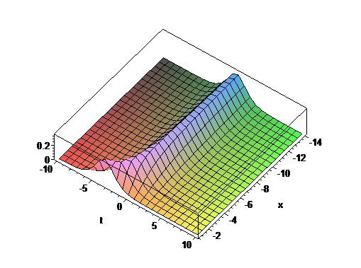
Figure 1: One-q-soliton solution $V$ of generalized $q$-Toda equation with $e^{\epsilon}=1.25,\alpha_{1}=-5,\beta_{1}=-1.1745$.

We pick the starting solution of eq.(23) as the assumption of two-soliton solutions.

$$f^{(1)}=2\cosh(-\frac{\alpha_{1}}{x}+\beta_{1}t+\eta_{1}),$$ (29)

where $\alpha_{i},\eta_{i},i=1,2$ are arbitrary constants with the related dispersion relation

$$\beta_{i}^{2}=e^{\alpha_{i}\epsilon}+e^{-\alpha_{i}\epsilon}-2,i=1,2.$$ (30)

Apparently the use of vector notation

$$p_{1}\pm p_{2}=(\beta_{1}\pm\beta_{2},\alpha_{1}\pm\alpha_{2},\eta_{1}\pm\eta_{2}),$$ (31)

can lead to dispersion relation eq.(30) as $P(p_{i})=0,i=1,2....$ Then we get

$$-P(\partial)f^{(2)}=[(\beta_{1}-\beta_{2})^{2}-(e^{(\alpha_{1}-\alpha_{2})\epsilon}+e^{(\alpha_{2}-\alpha_{1})\epsilon}-2)]e^{-\frac{\alpha_{1}+\alpha_{2}}{x}+(\beta_{1}+\beta_{2})t+\eta_{1}+\eta_{2}}.$$ (32)

Therefore, the form of $f^{(2)}$ can be

$$f^{(2)}=A(1,2)e^{-\frac{\alpha_{1}+\alpha_{2}}{x}+(\beta_{1}+\beta_{2})t+\eta_{1}+\eta_{2}}.$$ (33)

Substituting such $f^{(2)}$ into eq.(32) will help us determine the position of two-q-soliton as

$$A(1,2)=-\frac{(\beta_{1}-\beta_{2})^{2}-(e^{(\alpha_{1}-\alpha_{2})\epsilon}+e^{(\alpha_{2}-\alpha_{1})\epsilon}-2)}{(\beta_{1}+\beta_{2})^{2}-(e^{(\alpha_{1}+\alpha_{2})\epsilon}+e^{-(\alpha_{1}+\alpha_{2})\epsilon}-2)}=-\frac{P(p_{1}-p_{2})}{P(p_{1}+p_{2})}.$$ (34)

Supposing $f^{(3)}=0$, by the use of the dispersion relation eq.(30) the coefficient of $\varepsilon^{3}$ vanishes trivially and so do the rest of $\varepsilon^{j},j>3$. That means we have a good truncation up to $\varepsilon^{3}$ which leads to the two-q-soliton solution as

$$f(x,t)=1+e^{-\frac{\alpha_{1}}{x}+\beta_{1}t+\eta_{1}}+e^{-\frac{\alpha_{2}}{x}+\beta_{2}t+\eta_{2}}+A(1,2)e^{-\frac{\alpha_{1}+\alpha_{2}}{x}+(\beta_{1}+\beta_{2})t+\eta_{1}+\eta_{2}}.$$ (35)

Therefore, we illustrate the collision of two-q-solitons as Figure 2.

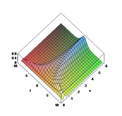
Figure 2: Two-q-soliton solution $V$ of generalized $q$-Toda equation with $e^{\epsilon}=1.25,\alpha_{1}=-5,\alpha_{2}=6.$

To further derive three-soliton solution, we choose the starting solution of eq.(23) as the assumption as

$$f^{(1)}=\sum\limits^{3}_{i=1}e^{-\frac{\alpha_{i}}{x}+\beta_{i}t+\eta_{i}},$$ (36)

where $\alpha_{i}$,$\eta_{i}$ are arbitrary constants for $i=1,2,3$. Similarly to the precious arguments, the coefficient of $\varepsilon^{0}$ vanishes trivially. From the coefficient of $\varepsilon^{1}$, we have the corresponding dispersion relation

$$\beta_{i}^{2}=e^{\alpha_{i}\epsilon}+e^{-\alpha_{i}\epsilon}-2,i=1,2,3.$$ (37)

From the coefficient of $\varepsilon^{2}$, we can obtain

$$-P(\partial)f^{(2)}=\sum\limits^{(3)}_{i<j}[(\beta_{i}-\beta_{j})^{2}-(e^{(\alpha_{i}-\alpha_{j})\epsilon}+e^{(\alpha_{i}-\alpha_{j})\epsilon}-2)]e^{-\frac{\alpha_{i}+\alpha_{j}}{x}+(\beta_{i}+\beta_{j})t+\eta_{i}+\eta_{j}}.$$ (38)

The equation eq.(38) implies the explicit form of $f^{(2)}$

$$f^{(2)}=\sum\limits^{(3)}_{i<j}A(i,j)e^{-\frac{\alpha_{i}+\alpha_{j}}{x}+(\beta_{i}+\beta_{j})t+\eta_{i}+\eta_{j}},$$ (39)

with

$$A(i,j)=-\frac{P(p_{i}-p_{j})}{P(p_{i}+p_{j})}=-\frac{(\beta_{i}-\beta_{j})^{2}-(e^{(\alpha_{i}-\alpha_{j})\epsilon}+e^{(\alpha_{i}-\alpha_{j})\epsilon}-2)}{(\beta_{i}+\beta_{j})^{2}-(e^{(\alpha_{i}+\alpha_{j})\epsilon}+e^{-(\alpha_{i}+\alpha_{j})\epsilon}-2)}.$$ (40)

For the coefficient of $\varepsilon^{3}$, we have

$$P(D)1\cdot f^{(3)}+f^{(3)}\cdot 1+f^{(1)}\cdot f^{(2)}+f^{(2)}\cdot f^{(1)}=0.$$

We can also rewrite them as

$$-P(\partial)f^{(3)} = (A(1,2)P(p_{3}-p_{1}-p_{2})+A(1,3)P(p_{2}-p_{1}-p_{3})+A(2,3)P(p_{1}-p_{2}-p_{3}))$$ (41)

$$\times e^{-\frac{\alpha_{1}+\alpha_{2}+\alpha_{3}}{x}+(\beta_{1}+\beta_{2}+\beta_{3})t+\eta_{1}+\eta_{2}+\eta_{3}}.$$

Suppose that $f^{(3)}$ is of the form

$$f^{(3)}=A(1,2,3)e^{-\frac{\alpha_{1}+\alpha_{2}+\alpha_{3}}{x}+(\beta_{1}+\beta_{2}+\beta_{3})t+\eta_{1}+\eta_{2}+\eta_{3}},$$ (42)

then one can find

$$A(1,2,3)=-\frac{A(1,2)P(p_{3}-p_{1}-p_{2})+A(1,3)P(p_{2}-p_{1}-p_{3})+A(2,3)P(p_{1}-p_{2}-p_{3})}{P(p_{1}+p_{2}+p_{3})}.$$ (43)

Following the steps, one can find we can suppose the vanishing of $f^{(4)}$ and it is a reasonable truncation to terms of $\varepsilon^{4}$, i.e. the from the equation eq.(22) becomes

$$2P(D)f^{(1)}\cdot f^{(3)}+P(Df^{(2)}\cdot f^{(2)}=0.$$ (44)

which means the following condition holds

$$A(1,2,3)=A(1,2)A(1,3)A(2,3).$$ (45)

Then we can express the solution of three-q-soliton(see Figure 3) as

$$\begin{split}f(x,t)=1+\sum\limits^{3}_{i=1}e^{-\frac{\alpha_{i}}{x}+\beta_{i}t+\eta_{i}}+\sum\limits^{3}_{i<j}A(i,j)e^{-\frac{\alpha_{i}+\alpha_{j}}{x}+(\beta_{i}+\beta_{j})t+\eta_{i}+\eta_{j}}\\ +A(1,2)A(1,3)A(2,3)e^{-\frac{\alpha_{1}+\alpha_{2}+\alpha_{3}}{x}+(\beta_{1}+\beta_{2}+\beta_{3})t+\eta_{1}+\eta_{2}+\eta_{3}}.\end{split}$$ (46)

 

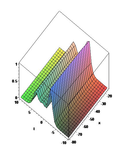
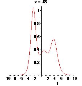
Figure 3: Three-q-soliton solution $V$ of generalized $q$-Toda equation with $e^{\epsilon}=1.25,\alpha_{1}=-5,\alpha_{2}=6.\alpha_{3}=-7.9141,\beta_{1}=-1.1745,\beta_{2}=-1.4411,\beta_{3}=2.0045$

The above three-soliton solutions show the great integrable possibility in a certain sense. To deeply prove the integrability, we will give the Lax pair of the generalized $q$-Toda hierarchy and further generalize it to a whole integrable hierarchy in the next section.

4 The  generalized $q$-Toda hierarchy

Now we will consider that the algebra of the shift operator $\Lambda_{\epsilon}:=e^{\epsilon x^{2}\partial_{x}}$. A Left multiplication by $X$ is as $X\Lambda_{\epsilon}^{j}$, $(X\Lambda_{\epsilon}^{j})(g)(x):=X(x)\circ g(\frac{x}{1-j\epsilon x})$ with defining the product $(X(x)\Lambda_{\epsilon}^{i})\circ(Y(x)\Lambda_{\epsilon}^{j}):=X(x)Y(\frac{x}{1-i\epsilon x})\Lambda_{\epsilon}^{i+j}.$

Now we introduce the following free operators $W_{0},\bar{W}_{0}$

$$W_{0} :=e^{\sum_{j=0}^{\infty}t_{j}\frac{\Lambda_{\epsilon}^{j}}{\epsilon j!}},$$ (47)

$$\bar{W}_{0} :=e^{-\sum_{j=0}^{\infty}t_{j}\frac{\Lambda_{\epsilon}^{-j}}{\epsilon j!}},$$ (48)

where $t_{j}\in\mathbb{R}$ will play the role of continuous times.

We define the dressing operators $W,\bar{W}$ as follows

$$W :=S\circ W_{0},\ \ \bar{W}:=\bar{S}\circ\bar{W}_{0},$$ (49)

where $S,\bar{S}$ have expansions as

$$\begin{aligned} S&=1+\omega_{1}(x)\Lambda_{\epsilon}^{-1}+\omega_{2}(x)\Lambda_{\epsilon}^{-2}+\cdots,\\ \bar{S}&=\bar{\omega}_{0}(x)+\bar{\omega}_{1}(x)\Lambda_{\epsilon}+\bar{\omega}_{2}(x)\Lambda_{\epsilon}^{2}+\cdots.\end{aligned}$$ (50)

The inverse operators $S^{-1},\bar{S}^{-1}$ of operators $S,\bar{S}$ have expansions of the form

$$\begin{aligned} S^{-1}&=1+\omega^{\prime}_{1}(x)\Lambda_{\epsilon}^{-1}+\omega^{\prime}_{2}(x)\Lambda_{\epsilon}^{-2}+\cdots,\\ \bar{S}^{-1}&=\bar{\omega}^{\prime}_{0}(x)+\bar{\omega}^{\prime}_{1}(x)\Lambda_{\epsilon}+\bar{\omega}^{\prime}_{2}(x)\Lambda_{\epsilon}^{2}+\cdots.\end{aligned}$$ (51)

The Lax operator $\mathcal{L}$ of the generalized $q$-deformed Toda hierarchy is defined by

$$\mathcal{L} :=W\circ\Lambda_{\epsilon}\circ W^{-1}=\bar{W}\circ\Lambda_{\epsilon}^{-1}\circ\bar{W}^{-1},$$ (52)

and have the following expansions

$$\begin{aligned} \mathcal{L}&=\Lambda_{\epsilon}+U(x)+V(x)\Lambda_{\epsilon}^{-1}.\end{aligned}$$ (53)

In fact the Lax operators $\mathcal{L}$ are also be equivalently defined by

$$\mathcal{L} :=S\circ\Lambda_{\epsilon}\circ S^{-1}=\bar{S}\circ\Lambda_{\epsilon}^{-1}\circ\bar{S}^{-1}.$$ (54)

4.1 Lax equations of the GQTH

In this section we will give the Lax equations of the GQTH. Let us firstly introduce some convenient notation such as the operators $B_{j}$ defined as $B_{j}:=\frac{\mathcal{L}^{j}}{j!}.$ Now we give the definition of the generalized $q$-Toda hierarchy(GQTH).

Definition 4.1.

The generalized $q$-Toda hierarchy is a hierarchy in which the dressing operators $S,\bar{S}$ satisfy following Sato equations

$$\epsilon\partial_{t_{j}}S =-(B_{j})_{-}S, \epsilon\partial_{t_{j}}\bar{S} =(B_{j})_{+}\bar{S}.$$ (55)

Then one can easily get the following proposition about $W,\bar{W}.$

Proposition 4.2.

The dressing operators $W,\bar{W}$ are subject to following Sato equations

$$\epsilon\partial_{t_{j}}W =(B_{j})_{+}W, \epsilon\partial_{t_{j}}\bar{W} =-(B_{j})_{-}\bar{W}.$$ (56)

From the previous proposition one can derive the following Lax equations for the Lax operators.

Proposition 4.3.

The Lax equations of the GQTH are as follows

$$\epsilon\partial_{t_{j}}\mathcal{L} =[(B_{j})_{+},\mathcal{L}].$$ (57)

To see this kind of hierarchy more clearly, the generalized $q$-Toda equations as the $t_{1}$ flow equations will be given in the next subsection.

4.2 The generalized $q$-Toda equations

As a consequence Sato equations, after taking into account that $S$ and $\bar{S}$, the $t_{1}$ flow of $\mathcal{L}$ in the form of $\mathcal{L}=\Lambda_{\epsilon}+U+V\Lambda_{\epsilon}^{-1}$ is as

$$\begin{aligned} \epsilon\partial_{t_{1}}\mathcal{L}&=[\Lambda_{\epsilon}+U,V\Lambda_{\epsilon}^{-1}],\end{aligned}$$ (58)

which lead to generalized $q$-Toda equation

$$\epsilon\partial_{t_{1}}U = V(\frac{x}{1-\epsilon x})-V(x),$$ (59)

$$\epsilon\partial_{t_{1}}V = U(x)V(x)-V(x)U(\frac{x}{1+\epsilon x}).$$ (60)

From Sato equation we deduce the following set of nonlinear partial differential-difference equations

$$\left\{\begin{aligned} \omega_{1}(x)-\omega_{1}(\frac{x}{1+\epsilon x})&=\epsilon\partial_{t_{1}}(e^{\phi(x)})\cdot e^{-\phi(x)},\\ \epsilon\partial_{t_{1}}\omega_{1}(x)&=-e^{\phi(x)}e^{-\phi(\frac{x}{1-\epsilon x})}.\end{aligned}\right.$$ (61)

Observe that if we cross the two first equations, then we get the generalized $q$-Toda equation (15). To give a linear description of the GQTH, we introduce wave functions $\psi,\bar{\psi}$ defined by

$$\begin{aligned} \psi&=W\cdot\chi,&\bar{\psi}&=\bar{W}\cdot\bar{\chi},\end{aligned}$$ (62)

where

$$\chi(z):=z^{-\frac{1}{x\epsilon}},\ \ \bar{\chi}(z):=z^{\frac{1}{x\epsilon}},\$$ (63)

and the $``\cdot"$ means the action of an operator on a function. Note that $\Lambda_{\epsilon}\cdot\chi=z\chi$ and the following asymptotic expansions can be defined

$$\begin{aligned} \psi&=(1+\omega_{1}(x)z^{-1}+\cdots)\,\psi_{0}(z),&\psi_{0}&:=z^{-\frac{1}{x\epsilon}}e^{\sum_{j=1}^{\infty}t_{j}\frac{z^{j}}{\epsilon j!}},\\ \bar{\psi}&=(\bar{\omega}_{0}(x)+\bar{\omega}_{1}(x)z+\cdots)\,\bar{\psi}_{0}(z),&\bar{\psi}_{0}&:=z^{\frac{1}{x\epsilon}}e^{-\sum_{j=0}^{\infty}t_{j}\frac{z^{-j}}{\epsilon j!}}.\end{aligned}$$ (64)

We can further get linear equations of the GQTH in the following proposition.

Proposition 4.4.

The wave functions $\psi,\bar{\psi}$ are subject to following Sato equations

$$\mathcal{L}\cdot\psi =z\psi,\ \ \ \mathcal{L}\cdot\bar{\psi}=z\bar{\psi},$$ (65)

$$\epsilon\partial_{t_{j}}\psi =(B_{j})_{+}\cdot\psi, \epsilon\partial_{t_{j}}\bar{\psi} =-(B_{j})_{-}\cdot\bar{\psi}.$$ (66)

5 Bi-Hamiltonian structure and tau symmetry

To describe the integrability of the GQTH, we will construct the Bi-Hamiltonian structure and tau symmetry of the GQTH in this section. In this section, we will consider the GQTH on Lax operator

$$\mathcal{L}=\Lambda_{\epsilon}+u+e^{v}\Lambda_{\epsilon}^{-1}.$$ (67)

Then for $\bar{f}=\int fdx,\bar{g}=\int gdx,$ we can define the hamiltonian bracket as

$$\{\bar{f},\bar{g}\}=\int\sum_{w,w^{\prime}}\frac{\delta f}{\delta w}\{w,w^{\prime}\}\frac{\delta g}{\delta w^{\prime}}dx,\ \ w,w^{\prime}=u\ or\ v.$$ (68)

The bi-Hamiltonian structure for the GQTH can be given by the following two compatible Poisson brackets similar as [2, 8]

$$\{v(x),v(y)\}_{1}=\{u(x),u(y)\}_{1}=0,$$

$$\{u(x),v(y)\}_{1}=\frac{1}{\epsilon}\left[e^{\epsilon\,x^{2}\partial_{x}}-1\right]\delta(x-y),$$ (69)

$$\{u(x),u(y)\}_{2}={1\over\epsilon}\left[e^{\epsilon\,x^{2}\partial_{x}}e^{v(x)}-e^{v(x)}e^{-\epsilon x^{2}\partial_{x}}\right]\delta(x-y),$$

$$\{u(x),v(y)\}_{2}={1\over\epsilon}u(x)\left[e^{\epsilon\,x^{2}\partial_{x}}-1\right]\delta(x-y),$$ (70)

$$\{v(x),v(y)\}_{2}={1\over\epsilon}\left[e^{\epsilon\,x^{2}\partial_{x}}-e^{-\epsilon x^{2}\partial_{x}}\right]\delta(x-y).$$

For any difference operator $A=\sum_{k}A_{k}\Lambda_{\epsilon}^{k}$, define residue $ResA=A_{0}$. In the following theorem, we will prove the above Poisson structure can be as the the Bi-Hamiltonian structures of the GQTH.

Theorem 5.1.

The flows of the GQTH are Hamiltonian systems of the form

$$\frac{\partial u}{\partial t_{j}} = \{u,H_{j}\}_{1},\ \ j\geq 0.$$ (71)

They satisfy the following bi-Hamiltonian recursion relation

$$\{\cdot,H_{n-1}\}_{2}=n\{\cdot,H_{n}\}_{1}.$$

Here the Hamiltonians have the form

$$H_{j}=\int h_{j}(u,v;u_{x},v_{x};\dots;\epsilon)dx,\quad\ j\geq 1,$$ (72)

with

$$h_{j} = \frac{1}{j!}Res\,\mathcal{L}^{j}.$$ (73)

Proof 5.2.

The proof is similar as the proof in [2, 8]. Here we will prove that the flows $\frac{\partial}{\partial t_{n}}$ are also Hamiltonian systems with respect to the first Poisson bracket.

Suppose

$$B_{n}=\sum_{k}a_{n;k}\,\Lambda_{\epsilon}^{k},$$ (74)

and from

$$\frac{\partial\mathcal{L}}{\partial t_{n}}=[(B_{n})_{+},\mathcal{L}]=[-(B_{n})_{-},\mathcal{L}],$$ (75)

we can derive equation

$$\epsilon\frac{\partial u}{\partial t_{n}} = a_{n;1}(\frac{x}{1-\epsilon x})-a_{n;1}(x),$$ (76)

$$\epsilon\frac{\partial v}{\partial t_{n}} = a_{n;0}(\frac{x}{1+\epsilon x})e^{v(x)}-a_{n;0}(x)e^{v(\frac{x}{1-\epsilon x})}.$$ (77)

By the following calcuation

$$d\tilde{h}_{n}=\frac{1}{n!}\,d\,Res\left[\mathcal{L}^{n}\right]=\frac{1}{n!}\,Res\left[\mathcal{L}^{n}d\mathcal{L}\right]$$

$$=Res\left[a_{n;0}(x)du+a_{n;1}(\frac{x}{1+\epsilon x})e^{v(x)}dv\right],$$ (78)

it yields the following identities

$$\frac{\delta H_{n}}{\delta u}=a_{n;0}(x),\quad\frac{\delta H_{n}}{\delta v}=a_{n;1}(\frac{x}{1+\epsilon x})e^{v(x)}.$$ (79)

This agree with Lax equation

$$\frac{\partial u}{\partial t_{n}} = \{u,H_{n}\}_{1}={1\over\epsilon}\left[e^{\epsilon\,x^{2}\partial_{x}}-1\right]\frac{\delta H_{n}}{\delta v}={1\over\epsilon}(a_{n;1}(\frac{x}{1-\epsilon x})-a_{n;1}(x)),$$ (80)

$$\ \frac{\partial v}{\partial t_{n}} = \{v,H_{n}\}_{1}=\frac{1}{\epsilon}\left[1-e^{\epsilon\,x^{2}\partial_{x}}\right]\frac{\delta H_{n}}{\delta u}=\frac{1}{\epsilon}\left[a_{n;0}(\frac{x}{1+\epsilon x})e^{v(x)}-a_{n;0}(x)e^{v(\frac{x}{1-\epsilon x})}\right].$$ (81)

From the above identities we see that the flows $\frac{\partial}{\partial t_{n}}$ are Hamiltonian systems with the first Hamiltonian structure. The recursion relation follows from the following trivial identities

$$n\,\frac{1}{n!}\mathcal{L}^{n}=\mathcal{L}\,\frac{1}{(n-1)!}\mathcal{L}^{n-1}=\frac{1}{(n-1)!}\mathcal{L}^{n-1}\mathcal{L}.$$

Then we get,

$$na_{n;1}(x)=a_{n-1;0}(\frac{x}{1-\epsilon x})+ua_{n-1;1}(x)+e^{v}a_{n-1;2}(\frac{x}{1+\epsilon x})$$

$$=a_{n-1;0}(x)+u(\frac{x}{1-\epsilon x})a_{n-1;1}(x)+e^{v(\frac{x}{1-2\epsilon x})}a_{n-1;2}(x).$$

This further leads to

$$\{u,H_{n-1}\}_{2}=\{\left[\Lambda_{\epsilon}e^{v(x)}-e^{v(x)}\Lambda_{\epsilon}^{-1}\right]a_{n-1;0}(x)+u(x)\left[\Lambda_{\epsilon}-1\right]a_{n-1;1}(\frac{x}{1+\epsilon x})e^{v(x)}\}$$

$$=n\left[a_{n;1}(x)e^{v(\frac{x}{1-\epsilon x})}-a_{n;1}(\frac{x}{1+\epsilon x})e^{v(x)}\right].$$

This is exactly the recursion relation on flows for $u$. The similar recursion flow on $v$ can be similarly derived. Theorem is proved till now.

Similarly as [2], the tau symmetry of the GQTH can be proved in the following theorem.

Theorem 5.3.

The GQTH has the following tau-symmetry property:

$$\frac{\partial h_{m}}{\partial t_{n}}=\frac{\partial h_{n}}{\partial t_{m}},\quad\ m,n\geq 1.$$ (82)

Proof 5.4.

Let us prove the theorem in a direct way

$$\frac{\partial h_{m}}{\partial t_{n}}=\frac{1}{m!\,n!}\,Res[-(\mathcal{L}^{n})_{-},\mathcal{L}^{m}]$$

$$=\frac{1}{m!\,n!}\,Res[(\mathcal{L}^{m})_{+},(\mathcal{L}^{n})_{-}]$$

$$=\frac{1}{m!\,n!}\,Res[(\mathcal{L}^{m})_{+},\mathcal{L}^{n}]=\frac{\partial h_{n}}{\partial t_{m}}.$$ (83)

Theorem is proved.

This property justifies the definition of the tau function for the GQTH as in the following proposition.

Proposition 5.5.

The $tau$ function of the GQTH can also be defined by the following expressions in terms of the densities of the Hamiltonians:

$$h_{n}=\epsilon(\Lambda_{\epsilon}-1)\frac{\partial\log\tau}{\partial t_{n}},\quad\ n\geq 0.$$ (84)

References

[1]
G. Carlet, The extended bigraded Toda hierarchy, J. Phys. A39
(2006) 9411–9435.
[2]
G. Carlet, B. Dubrovin, Y. Zhang, The Extended Toda Hierarchy,
Moscow Mathematical Journal4 (2004) 313–332,.
[3] B. A.
Dubrovin, Geometry of 2D topological field theories, in
Integrable systems and quantum groups (Montecatini Terme,
1993) 120–348, Lecture Notes in Math.1620 (Springer, Berlin,
1996).
[4]J. S. He, Y. H. Li, Y. Cheng, -deformed KP hierarchy and -deformed constrained KP hierarchy. SIGMA2(2006) 060.
[5] P. Iliev, Tau function solutions to a -deformation of the KP hierarchy,
Lett. Math. Phys.44(1998), 187-200.
[6] H. F. Jackson, -Difference equations, Am. J. Math.32(1910) 305–314.
[7] V. G. Kac and J. W. van de Leur, The n-component KP hierarchy and representation theory, J. Math. Phys.44 (2003) 3245.
[8] C. Z. Li, Sato theory on the -Toda hierarchy and its extension, submitted.
[9] C. Z. Li, Solutions of bigraded Toda hierarchy,
Journal of Physics A44(2011) 255201.
[10] C. Z. Li, J. S. He, On the extended -Toda hierarchy, arXiv:1403.0684.
[11]
C. Z. Li, J. S. He, Dispersionless bigraded Toda hierarchy and its additional symmetry, Reviews in Mathematical Physics24(2012) 1230003.
[12]
C. Z. Li, J. S. He, Y. C. Su, Block type symmetry of bigraded Toda hierarchy,
J. Math. Phys.53(2012) 013517.
[13]
C. Z. Li, J. S. He, K. Wu, Y. Cheng, Tau function and Hirota bilinear equations for the extended bigraded Toda
Hierarchy, J. Math. Phys.51(2010) 043514.
[14] C. Z. Li, T. T. Li, Virasoro symmetry of the -component q-constrained KP hierarchy, submitted.
[15]R. Lin, X. Liu, Y. Zeng, A new extended q-deformed KP hierarchy, Journal of Nonlinear Mathematical Physics, 15(2008) 333–347.
[16]J. Mas, M. Seco, The algebra of -pseudodifferential symbols and the - algebra,
J. Math. Phys.37(1996) 6510–6529.
[17]B. Silindir, Soliton solutions of -Toda lattice by Hirota
direct method, Advances in Difference Equations (2012) 2012:121.
[18]K. L. Tian, J. S. He, Y. C. Su, Y. Cheng, String equations of the -KP
hierarchy, Chinese Annals of Mathematics, Series B32(2011) 895–904.
[19]
M. Toda, Vibration of a chain with nonlinear interaction, J. Phys. Soc.
Jpn.22(1967) 431–436.
[20]
M. Toda, Nonlinear waves and solitons(Kluwer Academic Publishers,
Dordrecht, Holland, 1989).
[21]
Z. Tsuboi, A. Kuniba, Solutions of a discretized Toda field equation
for from analytic Bethe ansatz, J. Phys. A29(1996) 7785–7796.
[22]M. H. Tu, -deformed KP hierarchy: its additional
symmetries and infinitesimal Bäcklund transformations, Lett.
Math. Phys.49(1999) 95–103.
[23]K. Ueno, K. Takasaki, Toda lattice hierarchy,
In “Group representations and systems of differential
equations” (Tokyo, 1982) 1–95, Adv. Stud. Pure Math. 4,
(North-Holland, Amsterdam, 1984).
[24]
E. Witten, Two-dimensional gravity and intersection theory on moduli
space, Surveys in differential geometry1(1991) 243–310.