Systematic Shifts for Ytterbium-ion Optical Frequency Standards

Abstract

The projected systematic uncertainties of single trapped Ytterbium-ion optical frequency standards are estimated for the quadrupole and octupole transitions which are at wavelengths 435.5 nm and 467 nm, respectively. Finite temperature of the ion and its interaction with the external fields introduce drift in the measured frequency compared to its absolute value. Frequency shifts due to electric quadrupole moment, induced polarization and excess micromotion of the ion depend on electric fields, which are estimated in this article. Geometry of the trap electrodes also result in unwanted electric fields which have been considered in our calculation. Magnetic field induced shift and Stark shifts due to electro-magnetic radiation at a surrounding temperature are also estimated. At CSIR-NPL, we are developing a frequency standard based on the octupole transition for which the systematic uncertainties are an order of magnitude smaller than that using the quadrupole transition, as described here.

I Introduction

Recent advances in trapping and laser control of single ion has started a new era for frequency standards Wineland_RMP_2013 in optical frequency region, which can achieve 2-3 orders higher accuracy and lower systematic uncertainty Chou_PRL_2010 than current microwave clocks based on Cesium fountains Guena_IEEE_2012 ; PArora_IEEE_2013 . Realization of more accurate frequency standards will open up possibilities of vastly higher speed communication systems and more accurate satellite navigation systems besides enabling more precise verification of fundamental physical theories, in particular related to general relativity Chou_Science_2010 , cosmology SGTuryshev_Cosmology , and unification of the fundamental interactions SGKarshenboim_EPJ_2008 . So far a number of different ion species have been studied as promising optical frequency standards at several research institutes worldwide. These are ¹⁹⁹Hg⁺ at NIST, USA Rosenband_Science_2008 ; ¹⁷¹Yb⁺ at NPL, UK Gill_IEEE_2003 $\&$ PTB, Germany Tamm_PRA_2009 ; Huntemann_PRL_2012 ; ¹¹⁵In⁺ at MPQ, Germany Wang_OC_2007 ; ⁸⁸Sr⁺ at NRC, Canada Madej_PRA_2013 $\&$ NPL, UK Margolis_Science_2004 ; ⁴⁰Ca⁺ at CAS, China Gao_CSB_2013 $\&$ NICT, Japan Kajita_PRA_2005 and ²⁷Al⁺ at NIST, USA Chou_PRL_2010 . The accuracy of a frequency standard is decided by that of the measured atomic transition frequency, which may shift due to inter-species collisions and their interactions with external fields. Therefore, it is important to determine these systematic shifts precisely in order to improve the accuracy of the realized frequency standard.

At CSIR-NPL, India we are presently developing an optical frequency standards using Ytterbium-ion SDe_currentsc_2014 . It has a narrow $|^{2}\rm{S_{1/2};F=0,m_{F}=0}\rangle$-$|^{2}\rm{D_{3/2};F=2,m_{F}=0}\rangle$ quadrupole transition (E2) and an ultra-narrow $|^{2}\rm{S_{1/2};F=0,m_{F}=0}\rangle$-$|^{2}\rm{F_{7/2};F=3,m_{F}=0}\rangle$ octupole transition (E3) at wavelengths 435.5 nm and 467 nm, respectively OurNotation . These E2 and E3-transitions are at frequencies $\nu_{o}=688\,358\,979\,309\,306.62$ Hz Tamm_PRA_2009 and $642\,121\,496\,772\,645.15$ Hz Huntemann_PRL_2012 with natural line-widths 3.02 Hz and 1 nHz, respectively. We shall be probing the E3-transition in our frequency standards. The nuclear spin $I$=1/2 of ¹⁷¹Yb⁺ allows to eliminate the first-order Zeeman shift. The states associated with the E3-transition have the highest sensitivity to measure temporal constancy of fine structure constant and electron-to-proton mass ratio Margolis_ConPhys_2010 . In this article we have estimated five major sources of systematic uncertainties which are due to the electric quadrupole shift, Doppler shift, dc Stark shift, black-body radiation shift and Zeeman shift.

II Trapping of The Ytterbium-ion

A Paul trap Paul_Rev_1990 of end cap geometry Schrama_Optcomm_1993 as shown in Fig.1(a) will be employed for trapping single ¹⁷¹Yb⁺ ion SDe_currentsc_2014 . For a pure harmonic trapping potential $\Phi^{(k=2)}(x,y,z)$ the time dependent trajectory of the ions Werth_springer_2010 can be approximated as

$$u(t)\approx C\cos\bigg{(}\beta_{u}\frac{\omega_{rf}}{2}t\bigg{)}[1-\frac{q_{u}}{2}\cos(\omega_{rf}t)]$$ (1)

where $u\in\{x,y,z\}$, $C$ is the amplitude of the motion, $\omega_{rf}$ is the applied rf, $\beta_{u}=\sqrt{a_{u}+q_{u}^{2}/2}$, for $a_{u}$ and $q_{u}\ll 1$. The stability parameters, $a_{u}$ and $q_{u}$ depend on the applied dc and ac voltages, respectively. For precision measurements, in a real trap the anharmonic potential $\Phi^{(k>2)}(x,y,z)$ SDe_currentsc_2014 are non-negligible. Only the even order multipoles contribute in the case of a cylindrically symmetric end cap trap and the dominating perturbation arise from the octupole term $\Phi^{(k=4)}(x,y,z)$. Neglecting the asymmetries, which may arise from misalignment of the electrodes and machining inaccuracies, the trapping potential can be written as,

$$\Phi(x,y,z) = \frac{V_{T}(t)}{2{R}^{2}}\bigg{[}c_{2}(2z^{2}-x^{2}-y^{2})-\frac{c_{4}}{{R}^{2}}(3x^{4}+3y^{4}$$ (2)

$$+ 8z^{4}-24x^{2}z^{2}-24y^{2}z^{2}+6x^{2}y^{2})\bigg{]}$$

where, $R=\sqrt{{{r_{0}}^{2}}/2+{z_{0}}^{2}}$, $V_{T}(t)=U+V\cos(\omega_{rf}t)$ in terms of the dc component $U$, ac component $V$ of the trapping voltage and the dimensionless coefficients $c_{2}$, $c_{4}$ depend on electrode geometry. We have simulated geometry dependent trap potential using a commercial software CPO_USA_2013 and characterized its nature for several trap geometries as given by Eq.(2). For the trap geometry shown in Fig. 1 the coefficients $c_{2}$ and $c_{4}$ have been estimated to be 0.93 and 0.11, respectively. The restoring force for trapping ions due to $\Phi^{(k=2)}$ produces an axial trap depth, $D_{z}(U,V,\omega_{rf})=U/2+m{z_{o}}^{2}{\omega}^{2}_{rf}{q_{z}}^{2}/16Q$ Werth_springer_2010 where $Q$ and $m$ are charge and mass of the ion, respectively. Figure 1 (b-d) shows variation of the axial trap depth, $D_{z}$ as a function of the control parameters $U$, $V$ $\&$ $\omega_{rf}$ such that $q_{z}=-16QVc_{2}/m{\omega}^{2}_{rf}$ and $a_{z}=32QUc_{2}/m{\omega}^{2}_{rf}$ lie in the stability region Werth_springer_2010 . Throughout this article we have considered radial coordinate $r$ in the $xy$-plane instead of $x,\,y$ coordinates, since the trap is axially symmetric.

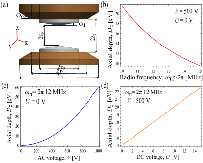
Figure 1: (a) The electrode assembly of our end-cap type Paul trap, where $2z_{0}\approx 0.6$ mm, $2z_{2}\approx 1.0$ mm, $2r_{1}=1$ mm, $2r_{2}=1.4$ mm, $2r_{3}=2$ mm, $\Theta_{i}=10^{\circ}$ and $\Theta_{o}=45^{\circ}$. (b), (c) and (d) show axial trap depth with respect to radio-frequency $\omega_{rf}$, ac $V$ and dc $U$ voltages respectively.

III Electric Quadrupole Shift

Electric quadrupole shift $\Delta\nu_{Q}$ of the atomic energy levels is one of the dominating systematic uncertainties for the precision frequency measurement. It arises due to the interaction of the atomic quadrupole moment $\Theta(\gamma,J)$ of a state having spectroscopic notation $\gamma$ and total angular momentum quantum number $J$ with the external electric field gradient $\nabla E$, giving a Hamiltonian as

$$H_{Q}=\nabla E\cdot\Theta=\sum^{2}_{q=-2}(-1)^{q}\nabla E_{q}\Theta_{-q}.$$ (3)

The quadrupole moment operator $\Theta$ and electric field gradient $\nabla E$ are tensors of rank two Ramsey_oxford_1956 . A non-zero atomic angular momentum results in a non-spherical charge distribution and the atom acquires a quadrupole moment. The ground state $\rm{|^{2}S_{1/2};0,0\rangle}$ of ${}^{171}\rm{Yb}^{+}$ has $\Theta(\rm{S},1/2)=0$, but the excited states $\rm{|^{2}D_{3/2};2,0\rangle}$ and $\rm{|^{2}F_{7/2};3,0\rangle}$ contributes to $\Delta\nu_{Q}$. The expectation value of $H_{Q}$ in reduced form, as given in Ref. Itano_Nist_2000 , is

$$\langle\gamma JFm_{F}|H_{Q}|\gamma JFm_{F}\rangle = \Theta(\gamma,J)\,\mathcal{F}_{Q}(I,J,F,m_{F})$$ (4)

$$\sum_{q=-2}^{2}\nabla E_{q}D_{0q},$$

where $D_{0q}$ are rotation matrix elements for projecting components of $\nabla E$ from the principle axes frame that is defined by the trap axes to the lab frame which is defined by the quantization direction Edmonds_princeton_1974 and

$$\mathcal{F}_{Q}=(-1)^{I+J+F}(2F+1)\left(\begin{array}[]{ccc}F&2&F\\ -m_{F}&0&m_{F}\\ \end{array}\right)$$ (7)

$${\left(\begin{array}[]{ccc}J&2&J\\ -J&0&J\\ \end{array}\right)}^{-1}\left\{\begin{matrix}{}J&2&J\\ F&I&F\\ \end{matrix}\right\}.$$ (10)

Here the quantities within $(\,)$, $\{\,\}$ are $3j$, $6j$-coefficients, respectively and $F$ is total angular momentum with its projection along the quantization axes $m_{F}$. The calculated $\mathcal{F}_{Q}$ for both $\rm{|^{2}D_{3/2};2,0\rangle}$ and $\rm{|^{2}F_{7/2};3,0\rangle}$ states is 1. Due to axial symmetry of the trap potential the contributions from $D_{0\pm 1}$ cancel with each other and $D_{00}=(3\cos^{2}\theta-1)/2$, $D_{0\pm 2}=\sqrt{3/8}\sin^{2}\theta(\cos 2\phi\mp i\sin 2\phi)$ contribute to Eq. 4, where $\theta$ and $\phi$ are Euler’s angles that rotates the principle axes frame and overlaps with the lab frame. The tensor components of $\nabla E$ can be calculated from $E_{x,y,z}$ produced by $\Phi(x,y,z)$ as described in Ref. Ramsey_oxford_1956 , which gives $\sum_{q}\nabla E_{q}D_{0q}=2V_{T}c_{2}[D_{00}-D_{02}/\sqrt{6}]$ and $12V_{T}c_{4}[4z^{2}(D_{00}-D_{02}/\sqrt{6})-x^{2}(2D_{00}-\sqrt{3/2}D_{02})]$ for harmonic and anharmonic potentials, respectively. The measured values of $\Theta(\gamma,J)$ for the $\rm{|^{2}D_{3/2};2,0\rangle}$ and $\rm{|^{2}F_{7/2};3,0\rangle}$ states of $\rm{{}^{171}Yb^{+}}$ are $2.08(11)ea_{o}^{2}$ Barwood_PRL_2004 and $-0.041(5)ea_{o}^{2}$ Huntemann_PRL_2012 respectively, where $e$ is electronic charge and $a_{o}$ is Bohr radius.

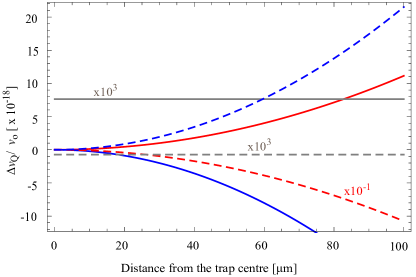
Figure 2: (Color online) Spatial dependence of the fractional electric quadrupole shifts $\Delta\nu_{Q}/\nu_{o}$ at the E2 and E3-clock transitions of $\rm{{}^{171}Yb^{+}}$, which are distinguished by solid and dashed lines, respectively. The quadrupole trapping potential produces a constant shift (gray) and the spatial dependence along the radial (red) and axial (blue) directions arise from the anharmonic components Figure .

The harmonic component of the trapping potential gives a constant electric field gradient however a spatial dependence comes from the anharmonic component, which introduces an uncertainty in the measured $\Delta\nu_{Q}$ due to motion of the ion. We estimate the quadrupole shift due to $U$ since the contribution from the $\rm{rf}$ averages to zero for first order electric quadrupole shift and for second order it is zero in case of $\rm{{}^{171}Yb^{+}}$ Schneider_PRL_2005 . Figure 2 shows the estimated fractional quadrupole shifts $\Delta\nu_{Q}/\nu_{0}$ due to $\Phi^{(2)}$ and $\Phi^{(4)}$ for the E2 and E3 - transitions of $\rm{{}^{171}Yb^{+}}$ respectively as a function of the radial and axial distance from the trap center. The shifts due to $\Phi^{(4)}$ computed for $\emph{U}=10$ V and $\theta=0^{\circ}$ are found to be three orders of magnitude smaller than the contribution due to $\Phi^{(2)}$, which are $\approx~{}5.25$ Hz and $\approx-0.51$ Hz for E2 and E3-transitions respectively and have no spatial dependence. The frequency shift can be cancelled in different ways as described in Ref. Madej_PRA_2013 , which could be opted depending on the system. The magnitude of the quadrupole shift is twice along the $z$-axis than they are along the $x,\,y$-axes but in opposite directions, respectively. We shall measure $\Delta\nu_{Q}$ separately by quantizing the ion along three mutually orthogonal directions of the principle axes, i. e. $\theta=0^{\circ}$, using magnetic fields of equal amplitude. Averaging these three would eliminate the total quadrupole shift Itano_Nist_2000 .

IV Doppler Shift

The relative motion between the laboratory and the ionic frames of reference introduces a shift in the observed frequency. The absorbed or emitted radiation $E_{o}\cos(\omega_{o}t)$ at frequency $\omega_{o}=2\pi\nu_{o}$ (wavelength $\lambda_{o}$) experiences a phase modulation $\eta\sin\omega_{s}t$ due to secular motion of the trapped ion at frequency $\omega_{s}$. The modulation depth $\eta=\Delta\omega_{o}/\omega_{s}$ depends on the Doppler shift $\Delta\omega_{o}=2\pi v/\lambda_{o}$ due to ion’s velocity $v=\omega_{s}r$. A modulated spectrum $E_{o}\cos(\omega_{o}t)\pm\eta E_{o}\cos(\omega_{o}\pm\omega_{s})t$ is expected when the ion is confined within $r<\lambda_{o}$ Dicke_PR_1953 , which is generally observed in an absorption spectroscopy for a narrow transition Berguist_PRA_1987 . This allows accurate determination of the first order Doppler unshifted $\nu_{o}$ for a laser cooled ion. However the second order Doppler effect introduces a frequency shift, which is given by

$$\frac{\Delta\nu_{D2}}{\nu_{o}}=-\frac{v^{2}}{2c^{2}}=\frac{2\varepsilon_{k}}{mc^{2}}$$ (11)

for kinetic energy $\varepsilon_{k}$ of the ion; $c$ is speed of light. For a laser cooled ion at 1 mK the fractional frequency uncertainty due to the temperature dependent second order Doppler effect is $\approx 10^{-19}$.

Figure 3: (Color online)Variation of the second order Doppler shifts with respect to the trap parameters - radio-frequency $\omega_{rf}$ (red), ac $V$ (blue) and dc $U$ (orange) voltages resulting from (a) temperature of the ion $T=1$ mK, (b) patch potential that ion experiences $E_{p}=1$ V/mm and (c) relative phase difference $\phi_{o}=1^{\circ}$ of the rf at two electrodes Figure .

Velocity of the trapped ion can be calculated from its trajectory, which gets deviated from Eq.(1) due to slowly varying stray electric fields. This can result from the patches of unwanted atoms on the electrode surface and relative phase differences of the rf on them. Over the time, Tantalum electrodes get coated with ${}^{171}\rm{Yb}$ atoms coming out of the oven. The differential work-function of Ytterbium and the Tantalum results in an electric field $\vec{E}_{p}$, which varies slowly with the deposition of atoms. As a result of an extra force, $Q\vec{E}_{p}$, the minimum of the confining potential shifts by an amount $C_{o}=Q\vec{E}_{p}\cdot\hat{u}/(m\omega_{s}^{2})$ and the micromotion increases Berkeland_JAP_1998 . A difference in path lengths and non-identical dimensions of the electrodes introduce a phase difference $\phi_{o}$ between the rf on the electrodes as $V\cos(\omega_{rf}t\pm\phi_{o}/2)$. For small $\phi_{o}$, i. e., $\sin\phi_{o}=\phi_{o}$ one can approximate this as two parallel plates separated by $2z_{o}/\alpha$ and at potentials $\pm V\phi_{o}\sin(\omega_{r}ft)/2$ which are subjected in addition to the rf, where the geometric factor $\alpha\approx 0.8$ for trap geometries satisfying $r_{o}^{2}=2z_{o}^{2}$ Gabrielse_PRA_1984 ; Beaty_PRA_1986 . For our trap geometry this generates an extra ac electric field $V\phi_{o}\alpha/2z_{o}\times\sin(\omega_{rf}t)\hat{z}$ which increases micromotion along the axial direction.

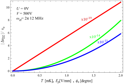
Figure 4: (Color online) Fractional second order Doppler shift $\Delta\nu_{2D}/\nu_{o}$ with: temperature $T$ (red); patch potential generated electric field $E_{p}$ (green) and phase difference $\phi_{o}$ of rf at the electrodes (blue) Figure .

Additional electric fields subject ion to excess force hence the ion trajectory gets modified as

$$u(t) \cong [C_{0}+C\cos(\omega_{rf}t)]\bigg{[}1+\frac{q_{u}}{2}\cos(\omega_{rf}t)\bigg{]}$$ (12)

$$- \frac{1}{4}q_{u}z_{0}\alpha\phi_{0}\sin(\omega_{rf}t)\delta_{u,z}.$$

where $\delta_{u,z}$ is Kronecker delta. This gives excess kinetic energy to the ion as described in Ref. Berkeland_JAP_1998 . The average kinetic energy of the ion is

$$\varepsilon_{k,u} = \frac{1}{4}mC^{2}\bigg{[}\omega_{s}^{2}+\frac{1}{8}q_{u}^{2}{\omega_{rf}}^{2}\bigg{]}+\frac{4}{m}\bigg{[}\frac{Qq_{u}\vec{E}_{p}\cdot\hat{u}}{(2a_{u}+q_{u}^{2})\omega_{rf}}\bigg{]}^{2}$$ (13)

$$+ \bigg{[}\frac{m(q_{u}z_{0}\alpha\phi_{o}\omega_{rf})^{2}}{64}\bigg{]}\delta_{u,z}$$

where the first term depends on temperature of the ion and remaining two terms are due to the $\vec{E}_{p}$ and $\phi_{o}$, respectively. The fractional frequency shift which is independent of $\nu_{o}$ can be calculated using Eq.(11). Each component of $\Delta\nu_{D2}/\nu_{o}$ depends on the trap parameters $\omega_{rf}$, $V$ and $U$ which are shown in Fig. 3. Figure 4 shows that $\Delta\nu_{2D}/\nu_{o}$ due to the patch potentials and ac phase difference at the two counteracting electrodes can produce orders of magnitude larger frequency shift than any other systematic effects. These are also discussed by Berkeland et. al. in Ref. Berkeland_JAP_1998 and by P. Gill in Ref. Gill_Metrologia_2005 . This concludes in order to build a frequency standard with fractional accuracy $~{}10^{-17}$, one has to control $\phi_{o}$ at a level $\approx 0.5$ milli-degree and $E_{p}<20$ mV/mm respectively. We shall employ two additional pairs of counteracting electrodes in the radial plane for cancelling stray potentials that ion experiences and the accurate machining will be essential for maintaining nearly zero path difference of the applied rf to the electrodes.

V DC Stark shift

Interaction of electric dipole moment (EDM) of an atom with an electric field results in Stark shift stark ; Itano_Nist_2000 of the atomic energy levels. The interaction energy is given as

$$H_{I}=-\vec{E}\cdot\vec{d},$$ (14)

where $\vec{E}$ is the electric field and $\vec{d}$ is the electric-dipole operator. As describe in Sec. IV in a real experiment the patch potentials lead to non zero dc electric fields at ion’s location and can introduce dc Stark shift. The electro-magnetic (EM) radiations at the non-zero temperature of the apparatus also introduces dc Stark shift which is known as black body radiation (BBR) shift. For ¹⁷¹Yb⁺ the first order Stark shift is zero because ion acquires a zero permanent EDM. The coupling of the ${}^{2}\rm{S}_{1/2}$, ${}^{2}\rm{D}_{3/2}$ and ${}^{2}\rm{F}_{7/2}$ states in ¹⁷¹Yb⁺ to all the other states via electric dipole interaction results to a non-zero second-order Stark shift which is not negligible. An induced EDM produces second order Stark shift stark as

$$\Delta\nu_{dc}=-\frac{1}{2h}\alpha E_{p}^{2},$$ (15)

where $h$ is the Plank constant, polarizability $\alpha$ has both scalar ($\alpha_{0}$) and tensor ($\alpha_{2}$) contributions. The effective $\Delta\nu_{dc}$ is calculated as the difference between the shifts of the states involved in the clock transition Itano_Nist_2000 ; fieqst as

$$\Delta\nu_{dc}=\frac{1}{4h}\left[2\Delta\alpha_{0}+\Delta\alpha_{2}(3\cos^{2}\theta-1)\right]E_{p}^{2},$$ (16)

where $\Delta\alpha_{0}$ and $\Delta\alpha_{2}$ are the polarizability differences of the states associated with the clock transition. The Stark shift becomes independent of $\Delta\alpha_{2}$ at $\theta=54.73^{\circ}$ but in our experiment $\theta\approx 0^{\circ}$ fixed by geometry of the apparatus. Here we estimate the second order Stark shifts resulting from dc electric field and EM-radiation.

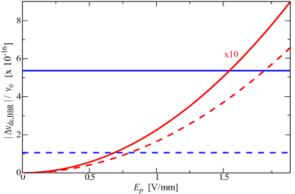
Figure 5: (Color online) Variation of the fractional dc Stark shift $\Delta\nu_{dc}/\nu_{o}$ with electric field $E_{p}$ (red) and the fractional BBR shift $\Delta\nu_{BBR}/\nu_{o}$ at 300 K (blue). E2 and E3-transitions are distinguished by solid and dashed lines, respectively Figure .

The Stark shift due to the $\Delta\alpha_{2}$ vanishes at the ground state because of its symmetric nature but not for the ²D_3/2 and ²F_7/2 states. Using the measured polarizibilities of the ²S_1/2, ²D_3/2 Schneider_PRL_2005 and ²F_7/2 Huntemann_PRL_2012 states variation of $\Delta\nu_{dc}/\nu_{o}$ with $E_{p}$ for the E2 and E3-transitions are shown in Fig. 5.

The electric field associated with the EM-radiation produced due to finite temperature of the apparatus and particularly the oven producing an atomic beam gives rise to BBR shift. The temperature dependent electric and magnetic fields are given by the Planck’s law bbr3 as

$$E^{2}(\omega)d\omega=B^{2}(\omega)d\omega=\frac{8\alpha^{3}}{\pi}\frac{\omega^{3}d\omega}{\exp(\frac{\omega}{k_{B}T})-1},$$ (17)

where $B$ is magnetic field, $\alpha$ is emissivity of the material and $\omega$ is frequency of EM-radiation. The wavelength corresponding to the maximum of the spectral energy density at 300 K is 9.7 $\mu$m microm , which is large compared to the longest transition wavelength $\approx$ 2.4 $\mu$m in ¹⁷¹Yb⁺. Therefore to a good approximation the BBR generated RMS amplitude of $E$ and $B$ fields are written as $\langle E^{2}\rangle=E_{o}^{2}\times(T/300)^{4}$ and $\langle B^{2}\rangle=B_{o}^{2}\times(T/300)^{4}$, where $E_{o}=831.9$ V/m and $B_{o}=2.775\times 10^{-6}$ T, respectively bbreq . The magnetic field contributes to a Zeeman shift, which will be discussed in the section VI. The contribution due to $\alpha_{2}$ can be neglected for an isotropic EM-radiation and the effective BBR shift can be written as

$$\Delta\nu_{BBR}=-\frac{1}{2h}\Delta\alpha_{0}\,E_{o}^{2}\left(\frac{T}{300}\right)^{4}.$$ (18)

At room temperature a shift of about 0.36 Hz and 0.068 Hz are estimated for the E2 and E3-transitions, respectively.

VI Zeeman Shift

Zeeman shift arises due to the interaction of atomic and nuclear magnetic moments $\mu_{J}$ and $\mu_{I}$ with an external magnetic field. In an experiment, magnetic field appears from the BBR, geomagnetic and stray fields. The E2 and E3-clock transitions are insensitive to the linear Zeeman effect since ground and excited states have $m_{F}=0$ states associated with them. Since the nuclear $g$-factor $g_{I}$ is much smaller than the electronic $g$-factor $g_{J}$, the second order Zeeman shift zeeman of the sublevels can be approximated only in terms of $g_{J}$ as

$$\Delta\nu_{\rm{QZ}}=-\left(\frac{g_{J}eB}{4\pi m}\right)^{2}\sum_{F^{\prime}}\frac{|\mathcal{F}_{Z}(I,J,F,F^{\prime},m_{F})|^{2}}{\Delta\nu_{HFS}},$$

where $\Delta\nu_{HFS}$ is the hyperfine splitting of the states and the matrix element $\mathcal{F}_{Z}=\langle F^{\prime},m^{\prime}_{F}|J_{z}|F,m_{F}\rangle$ zeeman1 is given as

$$\mathcal{F}_{Z} = \sqrt{I(I+1)(2I+1)(2F+1)(2F^{\prime}+1)}$$ (24)

$$\left(\begin{array}[]{ccc}F&1&F^{\prime}\\ -m_{F}&0&m_{F}\end{array}\right)\left\{\begin{array}[]{ccc}I&F&J\\ F^{\prime}&I&1\end{array}\right\}.$$

The calculated $|\mathcal{F}_{Z}|^{2}=1/4$ for the ²S_1/2, ²D_3/2 and ²F_7/2 states in ¹⁷¹Yb⁺. Their $g_{J}$ values are 1.998, 0.8021, 1.1429 and $\Delta\nu_{HFS}$ are 12.643 GHz, 0.86 GHz, 3.62 GHz, respectively NIST_database . The geomagnetic field in New Delhi, India is approximately $50~{}\mu$T which produces $\Delta\nu_{\rm{QZ}}$ of 38.75 Hz, 91.15 Hz, and 44.19 Hz at the ²S_1/2, ²D_3/2 and ²F_7/2 states, respectively. This results in a net second order Zeeman shift of 52.40 Hz and 5.44 Hz for the E2 and E3-clock transition, respectively. These are much larger than the shift produced by the magnetic field of the BBR at the room temperature whose values are $0.16$ Hz and $0.017$ Hz for the E2 and E3-transitions, respectively.

VII Conclusion

Table 1: Fractional shifts due to the systematic effects for the E2 and E3-transitions. The shifts are estimated at the room temperature $T=300$ K, rf phase difference $\phi_{o}=0.5$ mili-degree, stray electric and magnetic fields $E_{p}=20$ mV/mm and $B=1$ $\mu$T. Numerical values of $\phi_{o}$, $E_{p}$ and $B$ which are used here are typical values that can be achieved with proper minimization techniques.

Systematic	E2-transition	E3-transition
effect	[$\times 10^{-17}$]	[$\times 10^{-18}$ ]
Electric quadrupole	$762$	$-789$
Second order Doppler	$-1$	$-1$
dc Stark	$-0.09$	$-0.07$
BBR: dc Stark	$-52.3$	$-106$
Second order Zeeman	$-3.04$	$-3.39$
BBR: second order Zeeman	$-23.2$	$-26.4$

The systematic shifts from different source have been estimated for the E2 and E3-transitions of ¹⁷¹Yb⁺ and summarized in Tab. 1. Even though the electric quadrupole shift is the largest, averaging the measured frequency along three orthogonal directions effectively cancels $\Delta\nu_{Q}$. Three pairs of Helmholtz coils will be installed for defining the quantization axes. These coils will be used to cancel the static stray magnetic fields as well, for minimizing the quadratic Zeeman shift. The thermal part of $\Delta\nu_{D2}(T)$ is an order of magnitude smaller compared to the frequency standard that we aim for. Careful wiring for supplying rf and accurate machining of the electrodes is very important for making $\phi_{o}\approx 0^{\circ}$. Two pairs of electrodes will be installed in the radial plane for compensating the local electric fields that a trapped ion feels, which is required for minimizing $\Delta\nu_{D2}(E_{p})$ and $\Delta\nu_{dc}$. Surrounding temperature at the position of ion needs to be measured accurately Bloom_Nature_2014 for estimating the Stark and Zeeman shifts produced by BBR, which is the dominating systematic effect (Tab. 1). From our estimation, the E3-transition can provide an order of magnitude accurate frequency standards than the E2-transition of ¹⁷¹Yb⁺.

References

- (1) D. J. Wineland, Rev. Mod. Phys. 85, 1103 (2013) and references therein.
- (2) C. W. Chou, D. B. Hume, J. C. J. Koelemeij, D. J. Wineland, and T. Rosenband, Phys. Rev. Lett., 104, 070802 (2010).
- (3) J. Guena, M. Abgrall, D. Rovera, P. Laurent, B. Chupin, M. Lours, G. Santarelli, P. Rosenbusch, M. E. Tobar, R. Li, K. Gibble, A. Clairon, and S. Bize, IEEE Transactions on Ultrasonics, Ferroelectrics and Frequency Control 59, 391 (2012).
- (4) P. Aroroa, S. B. Purnapatra, A. Acharya, A. Agarwal, S. Yadav, K. Pant, A. Sen Gupta, IEEE Trans. Instrum. and Measurement 62, 2037 (2013).
- (5) C. W. Chou, D. B. Hume, T. Rosenband, and D. J. Wineland, Science 329, 1630 (2010).
- (6) From Quantum to Cosmos: Fundamental Physics Research in Space, S. G. Turyshev, World Scientific, Singapore (2009).
- (7) S. G. Karshenboim, and E. Peik, Eur. Phys. J. Special Topics 163, 1 (2008).
- (8) T. Rosenband, D. B. Hume, P. O. Schmidt, C. W. Chou, A. Brusch, L. Lorini, W. H. Oskay, R. E. Drullinger, T. M. Fortier, J. E. Stalnaker, S. A. Diddams, W. C. Swann, N. R. Newbury, W. M. Itano, D. J. Wineland, and J. C. Bergquist, Science 319, 1808 (2008).
- (9) P. Gill, G. P. Barwood, H. A. Klein, G. Huang, S. A. Webster, P. J. Blythe, K. Hosaka, S. N. Lea, and H. S Margolis, IEEE Meas. Sci. Technol. 14, 1174 (2003).
- (10) Chr. Tamm, S. Weyers, B. Lipphardt, and E. Peik, Phys. Rev. A, 80, 043403 (2009).
- (11) N. Huntemann, M. Okhapkin, B. Lipphardt, S. Weyers, Chr. Tamm, and E. Peik, Phys. Rev. Lett. 108, 090801 (2012).
- (12) Y. H. Wanga, R. Dumkea, T. Liua, A. Stejskala, Y. N. Zhaoa, J. Zhanga, Z. H. Lua, L. J. Wanga, Th. Beckerc, H. Waltherc, Opt. Comm. 273, 526 (2007).
- (13) P. Dube, A. A. Madej, Z. Zhou, and J. E. Bernard, Phys. Rev. A 87, 023806 (2013).
- (14) H. S. Margolis, G. P. Barwood, G. Huang, H. A. Klein, S. N. Lea, K. Szymaniec, and P. Gill, Science 306, 1355 (2004).
- (15) G. KeLin, Chinese Science Bulletin, 58, 853 (2013).
- (16) M. Kajita, Y. Li, K. Matsubara, K. Hayasaka, and M. Hosokawa, Phys. Rev. A 72, 043404 (2005).
- (17) S. De, N. Batra, S. Chakraborty, and S. Panja, A. Sen Gupta, accepted in Current Science (2014).
- (18) Throughout this manuscript, the atomic energy state total angular momentum and projection of it along the quantization axes defined by the applied magnetic field are contained within the ket.
- (19) H. S. Margolis, Contemp. Phys. 51, 37 (2010).
- (20) W. Paul, Rev. of Mod. Phys. 62, 531 (1990).
- (21) C. A. Schrama, E. Peik, W. W. Smith, and H. Walther, Opt. Com. 101, 32 (1993).
- (22) Charged Particle Traps, F. G. Major, V. N. Gheorghe, and G. Werth, Springer (2010).
- (23) 3D Charged Particle Optics program (CPO-3D), CPO Ltd., USA.
- (24) Molecular Beams, N. F. Ramsey, Oxford Univ. Press, London (1956).
- (25) W. M. Itano, J. Res. Nat. Inst. Stand. Tech., USA 105, 829 (2000).
- (26) Angular Momentum in Quantum Mechanics, A. R. Edmonds, Princeton Univ. Press (1974).
- (27) G. P. Barwood, H. S. Margolis, G. Huang, P. Gill, and H. A. Klein. Phys. Rev. Lett. 93, 133001 (2004).
- (28) T. Schneider, E. Peik, and Chr. Tamm, Phys. Rev. Lett. 94, 230801 (2005).
- (29) Multiplication factors, as indicated in the fugures, are used for accomodating multiple plots in a single figure.
- (30) R. H. Dicke, Phys. Rev. 89, 472 (1953).
- (31) J. C. Bergquist, Wayne M. Itano, and D. J. Wineland, Phys. Rev. A 36, 428 (1987).
- (32) D. J. Berkeland, J. D. Miller,J. C. Bergquist, W. M. Itano and D. J. Wineland, J. Appl. Phys. 83, 10 (1998).
- (33) G. Gabrielse, Phys. Rev. A 29, 462 (1984).
- (34) E. C. Beaty, Phys. Rev. A 33, 3645 (1986).
- (35) P. Gill, Metrologia 42, S125 (2005).
- (36) J. R. P. Angel and P. G. H. Sandars, Proc. Roy. Soc. A 305, 125 (1967).
- (37) J. R. P. Angel, P. G. H. Sandars, and G. K. Woodgate, J. Chem. Phys. 47, 1552 (1967).
- (38) E. J. Angstmann, V. A. Dzuba, and V. V. Flambaum, Phys. Rev. Lett. 97, 040802 (2006).
- (39) R. B. Warrington, Private communication.
- (40) J. W. Farley, and W. H. Wing, Phys. Rev. A 23, 2397 (1981).
- (41) Elementary Atomic Structure, G. K. Woodgate, 2nd ed. Oxford University Press, Oxford (1983).
- (42) Atomic Spectra and Radiative Transitions, I. I. Sobelman, Springer-Verlag, Berlin (1979).
- (43) NIST atomic spectra database, version 5, National Institute of Standards and Technology, USA.
- (44) B. J. Bloom, T. L. Nicholson, J. R. Williams, S. L. Campbell, M. Bishof, X. Zhang, W. Zhang, S. L. Bromley, and J. Ye, Nature 506, 71 (2014).