Dirac Structures in Vakonomic Mechanics
Abstract
In this paper, we explore dynamics of the nonholonomic system called vakonomic mechanics in the context of Lagrange-Dirac dynamical systems using a Dirac structure and its associated Hamilton-Pontryagin variational principle. We first show the link between vakonomic mechanics and nonholonomic mechanics from the viewpoints of Dirac structures as well as Lagrangian submanifolds. Namely, we clarify that Lagrangian submanifold theory cannot represent nonholonomic mechanics properly, but vakonomic mechanics instead. Second, in order to represent vakonomic mechanics, we employ the space , where a vakonomic Lagrangian is defined from a given Lagrangian (possibly degenerate) subject to nonholonomic constraints. Then, we show how implicit vakonomic Euler-Lagrange equations can be formulated by the Hamilton-Pontryagin variational principle for the vakonomic Lagrangian on the extended Pontryagin bundle . Associated with this variational principle, we establish a Dirac structure on to define an intrinsic vakonomic Lagrange-Dirac system. Furthermore, we establish another construction for the vakonomic Lagrange-Dirac system using a Dirac structure on , where we introduce a vakonomic Dirac differential. Lastly, we illustrate our theory of vakonomic Lagrange-Dirac systems by some examples such as the vakonomic skate and the vertical rolling coin.
Keywords and phrases: Dirac structures, vakonomic mechanics, nonholonomic mechanics, variational principles, implicit Lagrangian systems.
2000 Mathematics Subject Classification: 70H45, 70F25, 70Hxx, 70H30.
1 Introduction
Some Backgrounds.
In conjunction with optimal control design, much effort has been concentrated upon exploring geometric structures and variational principles of constrained systems (see, for instance, Lanczos [1949]; Arnold [1988]; Giaquinta and Hildebrandt [1996]; Jurdjevic [1997]; Marsden and Ratiu [1999]; Bloch [2003]). The motion of such constrained systems may be subject to a nontrivial distribution on a configuration manifold. For the case in which the given distribution is integrable in the sense of Frobenius’s theorem, the constraint is called holonomic, otherwise nonholonomic. It is well known that equations of motion for Lagrangian systems with holonomic constraints can be formulated by Hamilton’s variational principle by incorporating holonomic constraints into an original Lagrangian through Lagrange multipliers. On the other hand, Hamilton’s variational principle does not yield correct equations of motion for mechanical systems with nonholonomic constraints, but induces different mechanics instead. The correct equations of motion for nonholonomic mechanics can be developed from the Lagrange-d’Alembert principle. In other words, there are two different mechanics associated with systems with nonholonomic constraints. The first one is based on the Lagrange-d’Alembert principle and the corresponding equations of motion are called nonholonomic mechanics. The second one is called vakonomic mechanics (mechanics of variational axiomatic kind), which is purely variational and was developed by Kozlov [1983]; the name of vakonomic mechanics was coined by Arnold [1988]. Needless to say, both approaches are essentially different from the other: interesting comparisons between both of them can be found in Lewis and Murray [1995]; Cortés, de León, Martín de Diego, and Martínez [2003].
Nonholonomic mechanics has been studied from the viewpoints of Hamiltonian, Lagrangian as well as Poisson dynamics (see Koon and Marsden [1997]). Indeed, nonholonomic mechanics has many applications to engineering, robotics, control of satellites, etc., since it seems to be appropriate to model the dynamical behavior of phenomena such as rolling rigid-body, etc. (see Neimark and Fufaev [1972]). On the other hand, vakonomic mechanics appears in some problems of optimal control theory (related to sub-Riemannian geometry) (Bloch and Crouch [1993]; Brockett [1982]), economic growth theory (de León and Martín de Diego [1998]), motion of microorganisms at low Reynolds number (Koiler and Delgado [1998]), etc. A geometric unified approach was developed in de León, Marrero and Martín de Diego [2000].
In mechanics, one usually starts with a configuration manifold ; Lagrangian mechanics deals with the tangent bundle , while Hamiltonian mechanics with the cotangent bundle . It is known that nonholonomic and vakonomic mechanics can be described on extended spaces because of the presence of Lagrange multipliers. An interesting geometric approach to Lagrangian vakonomic mechanics on may be found in Benito and Martín de Diego [2005], while an approach on may be found in Martínez, Cortés and de León [2000]. In particular, since an extended Lagrangian on or is clearly degenerate, we have to explore its dynamics by using Dirac’s theory of constraints (see Dirac [1950]). Another interesting approach may be found in Cortés, de León, Martín de Diego, and Martínez [2003], where the authors depart from , and its submanifold , where , in order to develop an intrinsic description of vakonomic mechanics.
As shown in Yoshimura and Marsden [2006a], degenerate Lagrangian systems with nonholonomic constraints may be described, in general, by a set of implicit differential-algebraic equations, where a key point in the formulation of such implicit systems is to make use of the Pontryagin bundle , namely the fiber product (or Whitney) bundle . To the best of our knowledge, the Pontryagin bundle was first investigated in Skinner and Rusk [1983] to aid in the study of the degenerate Lagrangian systems, which is the case that we also treat in the present paper. The iterated tangent and cotangent spaces , , and and the relationships among these spaces were investigated by Tulczyjew [1977] in conjunction with the generalized Legendre transform, where a symplectic diffeomorphism plays an essential role in understanding Lagrangian systems in the context of Lagrangian submanifolds. The relation between these iterated spaces and the Pontryagin bundle was also discussed in Cendra, Holm, Hoyle and Marsden [1998]. Furthermore, Courant [1990b] investigated the iterated spaces , , and in conjunction with the tangent Dirac structures.
The notion of Dirac structures was developed by Courant and Weinstein [1998]; Dorfman [1987] as a unified structure of pre-symplectic and Poisson structures, where the original aims of these authors were to formulate the dynamics of constrained systems, including constraints induced from degenerate Lagrangians, as in Dirac [1950, 1964], where we recall that Dirac was concerned with degenerate Lagrangians, so that the image of the Legendre transformation, called the set of primary constraints in the language of Dirac, need not be the whole space. The canonical Dirac structures can be given by the graph of the bundle map associated with the canonical symplectic structure or the graph of the bundle map associated with the canonical Poisson structure on the cotangent bundle, and hence it naturally provides a geometric setting for Hamiltonian mechanics. It was already shown by Courant [1990a] that Hamiltonian systems can be formulated in the context of Dirac structures, however, its application to electric circuits and mechanical systems with nonholonomic constraints was studied in detail by van der Schaft and Maschke [1995], where they called the associated Hamiltonian systems with Dirac structures implicit Hamiltonian systems. On the other hand, Yoshimura and Marsden [2006a] explored on the Lagrangian side to clarify the link between an induced Dirac structure on and a degenerate Lagrangian system with nonholonomic constraints and they developed a notion of implicit Lagrangian systems as a Lagrangian analogue of implicit Hamiltonian systems. Moreover, the associated variational structure with implicit Lagrangian systems was investigated in Yoshimura and Marsden [2006b], where it was shown that the Hamilton-Pontryagin principle provides the standard implicit Lagrangian system. Another recent development that may be relevant with the Dirac theory of constraints was explored by Cendra, Etchechouryb and Ferraro [2011] by emphasizing the duality between the Poisson-algebraic and the geometric points of view, related to Dirac’s and of Gotay and Nester’s work.
Goals of the Paper.
The main purpose of this paper is to explore vakonomic mechanics, in the Lagrangian setting, both in the context of the Dirac structure and its associated variational principle called the Hamilton-Pontryagin principle. Another important point that we will clarify is the link between Dirac structures and Lagrangian submanifolds for the case of vakonomic mechanics. The organization of the paper is given as follows:
In §2, we will briefly introduce the geometric setting of the iterated tangent and cotangent bundles as well as the Pontryagin bundle. In §3, we will shortly review the Lagrangian submanifold theory for mechanics and will show that nonholonomic mechanics cannot be formulated on Lagrangian submanifolds, since the pullback of a symplectic two-form to the submanifold does not vanish. In §4 we will review Dirac structures in nonholonomic mechanics, by using the induced Dirac structure on the cotangent bundle and we will show how a degenerate Lagrangian system can be developed in the context of Dirac structures, together with the associated Lagrange-d’Alembert principle. In §5, we will consider the extended tangent bundle , where an extended Lagrangian , called vakonomic Lagrangian, is defined in association with a given Lagrangian on and with nonholonomic constraints. Then we will show that the vakonomic dynamics on can be obtained by the Hamilton-Pontryagin principle for , which yields the implicit vakonomic Euler-Lagrange equations. In parallel with this variational setting, taking advantage of the presymplectic structures constructed on , we will illustrate how the vakonomic analogue of the Lagrange-Dirac systems can be intrinsically developed by making use of the Dirac structure on . We shall also show another construction of the vakonomic Lagrange-Dirac system by employing a Dirac structure on . To do this, we make use of the Dirac differential of , where we introduce two maps and among the iterated bundles , and . It will be proved that the vakonomic Lagrange-Dirac system leads to the implicit vakonomic Euler-Lagrange equations. The section is closed with the main result of this paper, Theorem 5.11, where we summarize vakonomic mechanics can be formulated by Dirac structures as well as the Hamilton-Pontryagin variational principle. In §6, we will demonstrate our theory by some examples such as the vakonomic particle, the vakonomic skate and the vertical rolling disk on a plane. In §7, we will give some concluding remarks and future works.
Hamilton’s Principle for Holonomic Lagrangian Systems.
Before going into details, let us briefly recall the variational principle for constrained Lagrangian systems. First consider the case in which holonomic constraints are given. Let be a smooth dimensional manifold. Let be a Lagrangian and let be a constraint distribution on given for each as
where are independent one-forms that form the basis for the annihilator . In this paper, we assume that every distribution is regular, namely, it has constant rank at each point and is smooth unless otherwise stated. It follows from Frobenius’s theorem that is integrable or holonomic if for any vector fields on with values in , is a vector field that takes values in . Then, the submanifold may be described by a foliation such that, for each ,
where there exist smooth local functions as
and at each point in .
Let us define an extended Lagrangian by
where are the local coordinates of and are the Lagrange multipliers, which may be regarded as new variables. It follows from Hamilton’s principle that the stationarity condition for the action integral
induces equations of motion for the holonomic Lagrangian mechanical systems (see Giaquinta and Hildebrandt [1996]; Yoshimura [2008]):
Regarding the repeated indices such as in the above equations, we will employ Einstein’s summation convention in this paper unless otherwise noted.
Conventional Setting for Vakonomic Systems.
Let be a set of smooth functions, where , by which the constraints define a dimensional submanifold .
As in holonomic Lagrangian systems, let us define an extended Lagrangian by
| (1.1) |
Now, it is known that Hamilton’s principle for the action functional in the above does not provide correct equations of motion for the nonholonomic Lagrangian mechanical system, but some other dynamics called vakonomic mechanics (see Arnold [1988]). The correct equations of motion for nonholonomic Lagrangian mechanics can be given by Lagrange-d’Alembert principle.
Again, let be local coordinates for and consider the action functional given by
Keeping fixed the endpoints of the curve , i.e., and fixed, whereas and of are allowed to be free, the stationary condition of the above action functional provides the vakonomic Euler-Lagrange equations
which induce the usual equations of motion of vakonomic dynamics:
| (1.2) |
Now, let us illustrate the vakonomic setting with several applications.
Optimal Control Theory.
An optimal control problem is described by the following data (see de León, Martín de Diego, and A. Santamaría-Merino [2007]; Jiménez, Kobilarov and Martín de Diego [2013]): a configuration space giving the state variables of the system, a fiber bundle where fibers describe the control variables, a vector field along the projection , and a cost function . We consider the solutions of the optimal control problem the curves such that has fixed endpoints (that is, if is a curve, then and have fixed values), extremize the action functional
and satisfy the differential equation
which rules the evolution of the state variables.
It is easy to show that this is indeed a vakonomic problem on the manifold . The constraint submanifold , given by the above-mentioned differential equation, is defined by
The previous description of an optimal control problem determines the following commutative diagram:
In the above, is the canonical projection. Notice that plays the role of , the role of and the role of the Lagrangian function in the setting of vakonomic mechanics.
In conjunction with optimal control, we remark that Pontryagin’s maximum principle is the machinery that gives necessary conditions for solutions of optimal control problems (see Pontryagin, Boltyanskiĭ, Gamkrelidze and Mishchenko [1962]; Sussmann [1998]), which is relevant with variational principles for vakonomic dynamics in this paper.
Sub-Riemannian Geometry.
A sub-Riemannian structure on a manifold is a generalization of a Riemannian structure, where the metric is only defined on a vector subbundle of the tangent bundle. In such a case, the notion of length is only assigned to a subclass of curves, namely, curves with tangent vectors belonging to the vector subbundle at each point (see Langerock [2003]; Montgomery [2002]). More precisely, consider an -dimensional manifold equipped with a smooth distribution with constant rank at each point . A sub-Riemannian metric on consists of giving a positive definite quadratic form on smoothly varying in . We will say that a piecewise smooth curve is admissible if for all . Using the metric , it is possible to define the length
for admissible curves . From this definition, we can define the distance between two points as
if there exists admissible curves connecting and . A curve which realizes the distance between two points is called a minimizing sub-Riemannian geodesic. Let be a basis of one-forms for the annihilator . Then, an admissible path must verify the nonholonomic constraints
| (1.3) |
Therefore, it is clear that the problem to minimize sub-Riemannian geodesics is exactly the same as the vakonomic problem determined by the Lagrangian and with the nonholonomic constraints (1.3).
2 Iterated Tangent and Cotangent Bundles
In this section we recall some basic geometry of the spaces , and , as well as the Pontryagin bundle . These spaces are needed for the construction of Lagrangian mechanics on the tangent bundle and Hamiltonian mechanics on the cotangent bundle in the context of Lagrangian submanifold theory. In particular, there are two diffeomorphisms among , and that were originally developed by Tulczyjew [1977] for the generalized Legendre transform.
Diffeomorphism between and .
Now, we are going to define a natural diffeomorphism
In a local trivialization, is represented by an open set in a linear space , so that is represented by , while is locally given by . In this local representation, the map will be given by
where are local coordinates of and are the corresponding coordinates of , while are the local coordinates of induced by .
Consider the following two maps:
which are the obvious maps and recall that is the cotangent projection. The commutative condition used to define is the following diagram:
Namely,
Local Representation.
In a natural local trivialization, these maps are readily checked to be given by
Diffeomorphism between and .
Let be the canonical symplectic form on the cotangent bundle . There exists a natural diffeomorphism given by
which is the unique map that also intertwines two sets of maps:
Let be the tangent projection and the commutative condition for is given by the following diagram:
Namely,
Local Representations of Maps.
As before, in a local trivialization, is represented by , while is represented by . The map is locally represented by
Thus, the commutative diagram is verified in a local trivialization since one has
The Diffeomorphism between and .
With the elements previously defined, we can define a diffeomorphism between and , namely:
Using the local representation of and of , the map is locally given by
The Symplectic Form on .
The manifold is a symplectic manifold with a special symplectic form , which can be defined by two distinct ways as the exterior derivative of two intrinsic but different one-forms.
Now, there exist two one-forms and given by
where denotes the canonical one-form on and the canonical one-form on .
Using the local coordinates and of and , these two one-forms are denoted by
Thus, the symplectic form on associated with and can be defined by
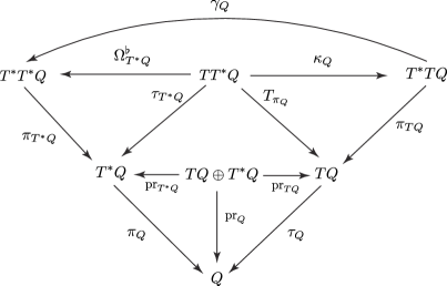
Pontryagin Bundle .
Consider the bundle over , that is, the Whitney sum of the tangent bundle and the cotangent bundle over , whose fiber at is the product . The bundle is called the Pontryagin bundle, see Yoshimura and Marsden [2006a]. Again, using a model space for and a chart domain, which is an open set , then is locally denoted by and by . In this local trivialization, the local coordinates of are written
Then, the following three projections are naturally defined:
All the previous developments may be summarized into the following diagram:
3 Lagrangian Submanifolds in Mechanics
As introduced in 2, the spaces , , are interrelated with each other by two symplectomorphisms and , which play essential roles in the construction of the generalized Legendre transformation originally developed by Tulczyjew [1977]. In this section, we shall see the theory of Lagrangian submanifolds using the geometry of these spaces. For the details, see, for instance, Weinstein [1971]; Abraham and Marsden [1978]; Weinstein [1979]; Liberman and Marle [1987]; Tulczyjew and Urbański [1999]; Yoshimura and Marsden [2006b].
Lagrangian Submanifolds.
Given a finite-dimensional symplectic manifold , and a submanifold with canonical inclusion , then is a Lagrangian submanifold if and only if and dimdim. If, locally, , then . So, it follows that there exists a function (defined locally) such that . We call a generating function of the Lagrangian submanifold . By the Poincaré lemma, locally this is always the case.
It is well known that the cotangent bundle of a given finite-dimensional smooth manifold , equipped with the symplectic two-form , is a symplectic manifold . Let be a closed one-form on . Then, the image of , namely , is a Lagrangian submanifold of , since . Thus, we obtain a submanifold diffeomorphic to and transverse to the fibers of . As to the details, see Abraham and Marsden [1978].
A useful extension of the previous construction is given by Tulczyjew [1977] in the following theorem.
Theorem 3.1 (Tulczyjew).
Let be a smooth manifold, and its tangent and cotangent bundle projections respectively. Let be a submanifold and a function. Then
is a Lagrangian submanifold of .
Here, we shall prove this theorem in a different way from Tulczyjew [1977]. Later, we will show the essential difference in geometry between vakonomic and nonholonomic mechanics by making use of this proof.
Proof.
Assume that , , are local coordinates for . Assume also that , , are adapted local coordinates for . Using these local coordinates, it is easily shown that is a submanifold of with dimension equal to dim. On the other hand, the submanifold shall be defined by a set of constraints in the following way
| (3.1) |
To finish the proof, we need to show that , i.e., the symplectic two-form on , vanishes when we restrict it to . With this purpose, we take the Lie derivative of (3.1), which provides
| (3.2) |
where . Since for all , where , it follows from (3.2) that
where are Lagrange multipliers. From the previous equation it follows
Let us introduce the inclusion map . Using Darboux’s coordinates for , one has . By a direct computation, we arrive to
since . This finishes the proof. ∎
Vakonomic Lagrangian Submanifolds.
Next, we see how the vakonomic mechanics introduced in 1 may be fit into the context of the Lagrangian submanifold theory. Particularly, in Tulczyjew’s theorem, setting , and , we can develop a submanifold of as
Consider the submanifold defined by the vanishing of the local constraints as
Hence
Note that the above constraints allow us to consider nonlinear nonholonomic constraints. Let be the inclusion of the submanifold; one can take an arbitrary extension such that . Applying theorem 3.1 we obtain
| (3.3) |
By definition this is a Lagrangian submanifold. Recall the local expression of the diffeomorphism ; namely,
we can construct the Lagrangian submanifold as
| (3.4) |
The solution curve for the dynamics determined by is given by such that
It is apparent that this verifies the set of differential-algebraic equations in (1.2).
Thus, the Lagrangian submanifold encloses the vakonomic mechanics, which we shall call the vakonomic Lagrangian submanifold. An analogous discussion can be found in Jiménez, de León and Martín de Diego [2012].
The Lagrange-d’Alembert Principle for Nonholonomic Mechanics.
Let us now formulate the nonholonomic mechanics by using the Lagrange-d’Alembert Principle. Let be a regular distribution given by
| (3.5) |
where the one-forms are nonintegrable. Note that we consider the case of linear constraints. Given a Lagrangian function , the dynamics of the nonholonomic mechanical system is determined by the Lagrange-d’Alembert principle, which states that a curve is an admissible motion of the system if
where we choose variations that satisfy at each and with the endpoints of fixed. Assume that at each point . Since the annihilator is generated by a set of independent one-forms as
the equations of motion of the nonholonomic mechanics are locally given by
| (3.6) |
where are Lagrange multipliers.
Nonholonomic Dynamical Submanifolds.
The dynamics of a mechanical system with nonholonomic constraints (3.5) may be represented by a submanifold
The main difference with the previous case is that the lifted distribution is given by
Recall at this point that the input data defining the nonholonomic dynamics is a Lagrangian function and a regular distribution , whose annihilator is spanned by the independent one-forms . Similar to the definition of the vakonomic Lagrangian submanifold (3.4), we can define the nonholonomic dynamical submanifold as
| (3.7) |
The solution curve for the dynamics represented by is given by such that
and the induced curve defined by verifies that
where is the Legendre transformation associated with . Locally, must satisfy equations (3.6). Therefore, encloses the nonholonomic dynamics (see also Jiménez, de León and Martín de Diego [2012]).
Now, we have the following proposition for the nonholonomic dynamical submanifold.
Proposition 3.2.
The nonholonomic dynamical submanifold is not a Lagrangian submanifold of .
Proof.
To prove this proposition, recall that the iterated tangent bundle has a symplectic structure defined by , which has the local form , where are local coordinates for .
Using local coordinates, it is clear to see that dim dim. Let
be the inclusion defined in (3.7) and we have to check if does not hold in order to accomplish the proof. By direct computations, it leads to
It follows from symmetric properties that this reduces to
Thus we conclude since in general . ∎
This last result implies that nonholonomic dynamics cannot be described in terms of Lagrangian submanifolds as we claimed.
Remark.
Poisson and almost-Poisson manifolds have been widely used in the geometrical description of nonholonomic mechanics (see for instance Cantrijn, de León and Martín de Diego [1999], Ibort, de León, Marrero and Martín de Diego [1998], Koon and Marsden [1998]). A different notion of Lagrangian submanifold (based in Liberman and Marle [1987] and Vaisman [1994]) has been developed in de León, Martín de Diego and Vaquero [2012] in the context of almost-Poisson geometry in order to construct a universal Hamilton-Jacobi theory including nonholonomic mechanics.
Remark.
As shown in equations (1.2) and (3.6), dynamical equations of both vakonomic and nonholonomic mechanics are clearly different, which comes from the fact that vakonomic mechanics can be a Lagrangian submanifold while nonholonomic mechanics cannot. This difference is clarified from the viewpoint of variational principles; namely, vakonomic mechanics is purely variational since we impose the constraints on the class of curves before applying the variations, while the nonholonomic mechanics is not variational since we impose the constraints to variations of curves after taking variations for the action integral. In other words, for the vakonomic mechanics, the admissible trajectories must lie in and the admissible variations must be tangent to , while for the nonholonomic mechanics, the admissible variations are generated by infinitesimal variations such that their vertical lift takes values in . Of course, this reflects the fact that nonholonomic mechanics is the one describing the actual motion of the mechanical systems with nonholonomic constraints, while vakonomic mechanics is not. For this perspective, see also Gracia, Martin-Solano, Munoz-Lecanda [2003] and Jozwikowski and Respondek [2013] and references therein. For a historical review on this topic, see de León [2012].
4 Dirac Structures in Nonholonomic Mechanics
As shown in the previous section, nonholonomic mechanics cannot be represented by Lagrangian submanifolds. In this section, we shall show how nonholonomic mechanics can be described in the context of induced Dirac structures and associated implicit Lagrangian systems, following Yoshimura and Marsden [2006a].
Dirac Structures.
We first recall the definition of a Dirac structure on a vector space , say finite dimensional for simplicity (see Courant [1990a] and Courant and Weinstein [1998]). Let be the dual space of , and be the natural paring between and . Define the symmetric paring on by
for . A Dirac structure on is a subspace such that , where is the orthogonal of relative to the pairing .
Now let be a given manifold and let denote the Pontryagin bundle over . A subbundle is called a Dirac structure on the bundle , when is a Dirac structure on the vector space at each point . A given two-form on together with a distribution on determines a Dirac structure on as follows111Precisely speaking, is called an almost Dirac structure, while for the case in which the distribution is integrable, is called a Dirac structure. In this paper, however, we simply call the Dirac structure unless otherwise stated..
Proposition 4.1.
The two-form determines a Dirac structure on whose fiber is given for each as
| (4.1) |
where and is the restriction of to .
Proof.
The orthogonal of at the point is given by
In order to prove that , let belong to . Then
since is skew-symmetric. Therefore, .
To conclude the proof we shall check that . Let . By definition of , we have that
for all and for all . Choose arbitrary vectors. From and the fact that is an arbitrary vector we have that
that is due to the skew-symmetry of . Thus, and hence , as required. Consequently, and the claim holds. ∎
Remark.
Of course, the proof above is also valid when and, furthermore, either for pre-symplectic or symplectic two-forms since the key property to accomplish the result is their skew-symmetry. On the other hand, throughout this work we shall define the Dirac structures in a different but equivalent way to proposition 4.1. Namely, each two-form on defines a bundle map by . Consequently, we may equivalently define in (4.1) as
We call a Dirac structure integrable if the condition
is satisfied for all pairs of vector fields and one-forms , , that take values in , where denotes the Lie derivative along the vector field on .
Induced Dirac Structures.
One of the most important and interesting Dirac structures in mechanics is the one that is induced from kinematic constraints, either holonomic or nonholonomic. This Dirac structure plays an essential role in the definition of implicit Lagrangian systems (or, alternatively, Lagrange-Dirac systems).
Let be a regular distribution on and define a lifted distribution on by
where is the canonical projection so that its tangent is a map . Let be the canonical two-form on . The induced Dirac structure on , is the subbundle of , whose fiber is given for each as
| (4.2) |
Local Representation of the Dirac Structure.
Let be local coordinates on so that locally, is represented by an open set . The constraint set defines a subspace of , which we denote by at each point . If we let the dimension of the constraint space be , then we can choose a basis of .
It is also common to represent constraint sets as the simultaneous kernel of a number of constraint one-forms; that is, the annihilator of , which is denoted by , is spanned by such one-forms, that we write as . Now writing the projection map locally as , its tangent map is locally given by . Thus, we can locally represent as
Let us denote a point in by , where is a covector and is a vector, notice that the annihilator of is locally,
Recall the symplectomorphism is given in local by
Thus, it follows from equation (4.2) that the local expression of the induced Dirac structure is given by
| (4.3) |
Lagrange-Dirac Dynamical Systems.
Following Yoshimura and Marsden [2006a, b], we shall briefly see the theory of Lagrange-Dirac systems. Let be a Lagrangian, possibly degenerate. The differential of is the one-form on locally given by
Using the canonical diffeomorphism , we define the Dirac differential of by
which is locally given by
where are local coordinates for , for and for .
Definition 4.2 (Lagrange-Dirac dynamical systems).
The equations of motion of a Lagrange-Dirac dynamical system (or an implicit Lagrangian system) are given by
| (4.4) |
Any curve satisfying (4.4) is called a solution curve of the Lagrange-Dirac dynamical system.
It follows from (4.3) and (4.4) that , is a solution curve if and only if it satisfies the implicit Lagrange-d’Alembert equations
| (4.5) |
Notice that the equations (4.5) are equal to the nonholonomic equations in (3.6).
Remark.
Note that the equation arises from the equality of the base points and in (4.4).
Energy Conservation for Implicit Lagrangian Systems.
Let be a Lagrange-Dirac dynamical system. Define the generalized energy function on by
If in is a solution curve of the Lagrange-Dirac system , then the energy is constant along the solution curve. This is shown as follows:
which vanishes since and since .
The Lagrange-d’Alembert-Pontryagin Principle.(Yoshimura and Marsden [2006b])
Let us see how the Lagrange-Dirac dynamical system can be developed from the Lagrange-d’Alembert-Pontryagin principle for a curve , in , which is given by
| (4.6) |
for chosen variations and with the constraint . Keeping the endpoints of fixed, we have
| (4.7) |
for variations , for all and , and with .
Thus, we obtain the local expression of the Lagrange-Dirac dynamical system in (4.5) from the Lagrange-d’Alembert-Pontryagin principle in (4.7).
For the case in which , this recovers the Hamilton-Pontryagin principle, which induces the implicit Euler-Lagrange equations.
Dirac Structures in Hamiltonian Systems.
In general, the standard Dirac structure on a manifold is given by the graph of a skew-symmetric bundle map over as shown above. The Hamilton-Dirac system can be given by a pair that satisfies, for each ,
| (4.8) |
where denotes a Hamiltonian. The idea was shown by van der Schaft and Maschke [1995] to the case of a nontrivial distribution on a Poisson manifold , which is called implicit Hamiltonian systems.
For the case , using the usual local coordinates leads to the canonical Dirac structure and the standard Hamiltonian system. The standard Hamiltonian equations can be also formulated by Hamilton’s phase space principle (see Yoshimura and Marsden [2006b]):
with the fixed endpoint conditions .
Intrinsically, Hamilton’s phase space principle is described by
where is a one-form on , which may induce under the condition of the variation of the curves fixed at the endpoints:
where . The above construction is clearly consisted with the construction using the canonical Dirac structure as in (4.8).
5 Lagrange-Dirac Systems in Vakonomic Mechanics
The Hamilton-Pontryagin Principle for Vakonomic Lagrangians.
Let us consider the Hamilton-Pontryagin principle for vakonomic Lagrangians. To do this, let be a Lagrangian, possibly degenerate, and consider the following nonholonomic constraints:
where are the local coordinates of .
Definition 5.1.
Define a vakonomic Lagrangian by
| (5.1) |
where is the usual Lagrangian and we consider as the local coordinates of the dual vector space . Define also the vakonomic Lagrangian energy by
where are local coordinates of the vakonomic Pontryagin bundle .
Proposition 5.2.
Let be a (possibly degenerate) Lagrangian function. Define the action functional
| (5.2) |
Keeping the endpoints of fixed, whereas the endpoints of , and are allowed to be free, the stationary condition for this action functional induces the local implicit vakonomic Euler-Lagrange equations:
| (5.3) |
which are restated by
| (5.4) |
Notice that the above equations are equivalent with (1.2).
Proof.
By direct computations, the variation of the action functional (5.2) is given by
where integration by parts has been taken into account. Keeping the endpoints of fixed, namely, , the stationarity condition for the action functional with free variations provides the set of equations (5.3), which lead to (5.4) straightforwardly from the definition of . ∎
We call the above variational principle as the Hamilton-Pontryagin principle for the vakonomic Lagrangian .
The Intrinsic Implicit Vakonomic Euler-Lagrange Equations.
Our next purpose is to develop an intrinsic form for the vakonomic Euler-Lagrange equations.
Let be the canonical one-form on and thus is the canonical two-form on . Define the projections
One can define a pre-symplectic form on by
| (5.5) |
In the above, notice that holds since is the one-form on . Thus, it follows
Definition 5.3.
Let be a curve in . Let us define the action functional for by
| (5.6) |
which is the intrinsic expression of (5.2).
Proposition 5.4.
Under the endpoints of fixed, the stationarity condition of the action functional (5.6) singles out a critical curve that satisfies the intrinsic implicit vakonomic Euler-Lagrange equations:
| (5.7) |
Proof.
The stationarity condition of the action functional is given by
for all variations with the endpoints of fixed. Thus, one obtains equation (5.7)
We call the above variational principle the Hamilton-Pontryagin principle for the vakonomic Lagrangian.
The Lagrange-Dirac Dynamical System on .
Recall that we can naturally define a presymplectic form on as in (5.5). Then, we can also define the associated bundle map
by, for ,
Definition 5.5.
Define the Dirac structure on by using the pre-symplectic two-form (5.5) as
Proposition 5.6.
The Vakonomic Dirac Differential Operator.
In the previous paragraph we have defined the vakonomic Lagrange-Dirac dynamical system in terms of the pair . Here, by analogy with the construction of implicit Lagrangian systems, we shall define an alternative notion of vakonomic Lagrange-Dirac system. To do this, we introduce the following isomorphisms:
and
where . Then, we define a diffeomorphism between and as
| (5.10) |
where is the identity map.
Given a vakonomic Lagrangian on , its differential is a one-form , which may be locally described by
Using the diffeomorphism in (5.10), we can define a differential operator called the vakonomic Dirac Differential of by
| (5.11) |
Namely, the map is locally given by
| (5.12) |
Pre-symplectic Form on
Using the natural projection
we can define a pre-symplectic structure on by
| (5.13) |
which is given in local form, for each , by
Associated with , we have the bundle map
which is locally denoted by
Dirac Structure on .
Before constructing the Lagrange-Dirac system for the vakonomic mechanics, we shall define a Dirac structure on as in the below.
Definition 5.7.
Define a Dirac structure on by using the pre-symplectic form in (5.13) as
Proposition 5.8.
The Dirac structure on is locally denoted, for each , by
| (5.14) |
where we denote
Proof.
Again, the claim follows from the particular local form of given by (5.13), namely . Therefore, if it follows that
which finishes the proof. ∎
The Vakonomic Lagrange-Dirac Systems on .
We give the definition of vakonomic Lagrange-Dirac systems on as follows:
Definition 5.9.
Let be a given Lagrangian function (possibly degenerate). Let , be a curve in . The equations of motion for the vakonomic Lagrange-Dirac system are given by
| (5.15) |
Proposition 5.10.
Proof.
By definition, we have
and hence it follows from (5.15) that, for the solution curve ,
Since on the left-hand side of the above equation, we obtain the implicit vakonomic Euler-Lagrange equations (5.16).
Locally, we have
while we recall that
such that the base point holds:
Therefore, we arrive to
which are equations (5.3). ∎
Needless to say, equations (5.16) are equal to the implicit vakonomic Euler-Lagrange equations in (5.7).
Now we have described the vakonomic dynamics from several points of view; namely, the Hamilton-Pontryagin variational principle as well as the intrinsic Lagrange-Dirac dynamical systems using Dirac structures. Our results may be summarized in the following theorem:
Theorem 5.11.
The following statements are equivalent:
-
1.
The Hamilton-Pontryagin principle for the following action integral
holds for any variations of with fixed endpoints.
-
2.
The curve , satisfies the implicit vakonomic Euler-Lagrange equations
which are locally given by
-
3.
The curve is a solution curve of the vakonomic Lagrange-Dirac dynamical system which satisfies
-
4.
The curve is a solution curve of the vakonomic Lagrange-Dirac dynamical system which satisfies
which is equivalent to
6 Examples
The Vertical Rolling Disk.
Let us consider the following problem for a disk of radius and unit mass which rolls on a horizontal plane. The configuration space for this system can be identified with . By we denote the coordinates of the point of contact of the disk with the plane and give, respectively, the angle between the disk and the axis, and the angle of rotation between a fixed diameter in the disk and the axis. Therefore, we will use the coordinate notation .
Given the endpoints of fixed, we want to find the trajectories of the disk connecting such points that minimize the energy consumption. Assume that the disk rolls on a plane without slipping, which is given by the following nonholonomic constraints:
As in 1, this is considered as an optimal control problem by setting , and . Using local coordinates , the cost function is given by the following Lagrangian :
where and denote the momenta of inertia.
In fact, in this framework we regard the velocities as the control variables. Solving this optimal control problem is precisely the same as the vakonomic problem associated to the vertical rolling disk for the vakonomic Lagrangian on by incorporating the nonholonomic constraints as
In the above, are Lagrange multipliers, where we set .
For each point , we employ the local coordinates
Then the Hamilton-Pontryagin principle for yields the equations of motion:
| (6.1) |
together with the nonholonomic constraints:
Next, we shall see how the vakonomic Lagrange-Dirac system can be constructed by using a Dirac structure on . Associated with the vakonomic Lagrangian on , its differential is a one-form , which may be locally described by
Then, the vakonomic Dirac differential of is denoted by
It follows from the condition of the vakonomic Lagrange-Dirac system, namely
that
where
Needless to say, the above matrix equation are equivalent with the implicit vakonomic Euler-Lagrange equations given in (6.1).
The Vakonomic Particle.
A particle of unit mass evolving in subject to the nonholonomic constraint . Using local coordinates the Lagrangian is given by , while the vakonomic Lagrangian is
For each point we employ the local coordinates
The Hamilton-Pontryagin principle for the vakonomic Lagrangian, we obtain the implicit vakonomic Euler-Lagrange equations are given by
together with the nonholonomic constraints
Now we construct the implicit vakonomic Lagrangian system using the Dirac structure . Noting
it follows from the condition
that the implicit vakonomic Euler-Lagrange equations are obtained as
where
The Vakonomic Skate.
Consider a plane with Cartesian coordinates of the contact point of the skate with the plane, and slanted at an angle (which is fixed). Let be an angle which denotes the orientation of the skate measured from the axis. Thus, we shall consider as the configuration manifold of this system. Suppose that the skate is moving under the gravitational force, where we denote by the acceleration due to gravity. Let and be the mass and the moment inertia of the skate about a vertical axis through its contact point respectively. The nonholonomic constraint is given by
while the mechanical Lagrangian reads
Using coordinates ,
the vakonomic Lagrangian reads
The Hamilton-Pontryagin principle for the vakonomic Lagrangian induces the implicit vakonomic Euler-Lagrange equations given by the following set of differential-algebraic equations:
together with the constraints
Now we construct the implicit vakonomic Lagrangian system using the Dirac structure . In this case, one has
and it follows from
that the implicit vakonomic Euler-Lagrange equations are obtained as
where
7 Conclusions and Future Works
We have explored vakonomic mechanics in the context of Dirac structures and its associated Lagrange-Dirac systems. First, we have shown that the Lagrangian submanifold theory cannot represent nonholonomic mechanics, but vakonomic mechanics can be properly described on a Lagrangian submanifold. Second, we have shown the Lagrange-Dirac dynamical formalism, especially, employing the symplectomorphisms among the iterated tangent and cotangent bundles , and . Then, we have defined a vakonomic Lagrangian on by incorporating nonholonomic constraints into a given Lagrangian on . Moreover, we have introduced its associated energy on the vakonomic Pontryagin bundle . Employing this energy, we have shown that the Hamilton-Pontryagin principle provides the implicit Euler-Lagrange equations for the vakonomic Lagrangian. We have also shown that one can develop a Dirac structure on and its associated vakonomic Lagrange-Dirac system, which yields the implicit vakonomic Euler-Lagrange equations. Furthermore, we have established another Dirac structure on by extending the formula given in Yoshimura and Marsden [2006a]. To do this, we have introduced the bundle maps and in order to define the Dirac differential for the vakonomic Lagrangian on . Finally, we have illustrated our theory by some examples such as the vakonomic particle, the vakonomic skate and the vertical rolling coin.
We hope that the framework of vakonomic Lagrange-Dirac mechanics proposed in this paper can be explored further. In particular, the following researches are of our concern for future work:
-
•
Symmetry reduction: We are interested in the vakonomic Lagrange-Dirac systems with symmetry (see for instance Martínez, Cortés and de León [2001]) and is our intention to establish a Dirac reduction theory for this.
-
•
Discrete vakonomic Lagrange-Dirac mechanics: In parallel with what we have done in the continuous setting of the vakonomic Lagrange-Dirac systems in this paper, its discrete analogue shall be developed.
-
•
Applications to optimal control problems: Due to the relationship of vakonomic mechanics and optimal control theory, and the applications of the latter to vehicles, space missions design, etc.; it is our aim to explore further vakonomic Lagrange-Dirac systems in this direction.
Acknowledgements.
We are very grateful to David Martin de Diego, Frans Cantrijn, Tom Mestdag and Franços Gay-Balmaz for useful remarks and suggestions. We also greatly appreciate Yoshihiro Shibata for his hearty supporting at Institute of Nonlinear Partial Differential Equations of Waseda University.
The research of F. J. was supported in its first part by Institute of Nonlinear Partial Differential Equations at Waseda University and was partially developed during his staying there in 2012 as a visiting Postdoctoral associate. In its second stage, the research of F. J. was supported by the DFG Collaborative Research Center TRR 109, ‘Discretization in Geometry and Dynamics’. The research of H. Y. is partially supported by JSPS Grant-in-Aid 26400408, JST-CREST, Waseda University Grant for SR 2012A-602 and IRSES project Geomech-246981.
References
- Abraham and Marsden [1978] Abraham, R. and J. E. Marsden [1978], Foundations of Mechanics. Benjamin-Cummings Publ. Co, Updated 1985 version, reprinted by Persius Publishing, second edition.
- Arnold [1988] Arnold, V. I.[1988], Dynamical Systems: Vol III. Springer-Verlag, New York.
- Benito and Martín de Diego [2005] Benito, R. and D. Martín de Diego [2005], Discrete vakonomic mechanics. J. Math. Phys., 46, 083521.
- Bloch [2003] Bloch, A. M. [2003], Nonholonomic Mechanics and Control, volume 24 of Interdisciplinary Applied Mathematics. Springer-Verlag, New York. With the collaboration of J. Baillieul, P. Crouch and J. Marsden, and with scientific input from P. S. Krishnaprasad, R. M. Murray and D. Zenkov.
- Bloch and Crouch [1993] Bloch, A. M. and P. E. Crouch [1993], Nonholonomic and vakonomic control systems on Riemannian manifolds, Dynamics and Control of Mechanical Systems. Fields Institute Communication 1. American Mathematical Society, Providence, RI, 25–52.
- Brockett [1982] Brockett, R. W. [1982], Control theory and singular Riemannian geometry. New Directions in Applied Mathematics, edited by P. J. Hilton and G. S. Young. Springer, New York, pp. 11–27.
- Cantrijn, de León and Martín de Diego [1999] Cantrijn F., de León M. and Martín de Diego D. [1999], On almost-Poisson structures in nonholonomic mechanics. Nonlinearity, 12, pp. 721-737.
- Cendra, Holm, Hoyle and Marsden [1998] Cendra, H., Holm, D. D., Hoyle, M. J. W. and J. E. Marsden [1998], The Maxwell-Vlasov equations in Euler-Poincaré form. J. Math, Phys. 39, pp. 3138–3157.
- Cendra, Etchechouryb and Ferraro [2011] Cendra, H., Etchechouryb, M., and S. J. Ferraro [2011], The Dirac theory of constraints, the Gotay-Nester theory and Poisson geometry. Preprint, arXiv: 1106.3354v1.
- Cortés, de León, Martín de Diego, and Martínez [2003] Cortés, J., de León, M., Martín de Diego, D. and Martínez, S. [2003], Geometric description of vakonomic and nonholonomic dynamics. Comparison of solutions. SIAM J. Control Optim. 41(5), pp. 1389–1412.
- Courant [1990a] Courant, T. J. [1990a], Dirac manifolds. Trans. Amer. Math. Soc. 319, pp. 631–661.
- Courant [1990b] Courant, T. J. [1990b], Tangent Dirac structures. J. Phys. A: Math. Gen. 23, pp. 5153–5168.
- Courant and Weinstein [1998] Courant, T. and A. Weinstein [1988], Beyond Poisson structures. In Action hamiltoniennes de groupes. Troisieme theoréme de Lie (Lyon, 1986), volume 27 of Travaux en Cours, pp. 39–49. Hermann, Paris.
- Dirac [1950] Dirac, P. A. M. [1950], Generalized Hamiltonian dynamics. Canadian J. Math. 2, pp. 129–148.
- Dirac [1964] Dirac P. A. M. [1964], Lectures on Quantum Mechanics, Belfer Graduate School of Science, Yeshiva University, New York.
- Dorfman [1987] Dorfman, I. [1987], Dirac structures of integrable evolution equations. Physics Letters A. 125(5), pp. 240-246.
- Giaquinta and Hildebrandt [1996] Giaquinta, M. and S. Hildebrandt [1996], Calculus of Variations I, volume 310 in Series of Comprehensive Studies in Mathematics, Springer-Verlag, Berlin Heidelberg.
- Gracia, Martin-Solano, Munoz-Lecanda [2003] Gracia, X., Martin-Solano, J. and Munoz-Lecanda, M. [2003], Some geometric aspects of variational calculus in constrained systems. Rep. Math. Phys. 51(1), pp. 127–148.
- Ibort, de León, Marrero and Martín de Diego [1998] Ibort A., de León M., Marrero J.C. and Martín de Diego D. [1998], A Dirac bracket for nonholonomic Lagrangian systems. Proc. V Fall Workshop: Geometry and Physics (Jaca, September 1996). Memorias de la Real Academia de Ciencias: Serie de Ciencias Exactas XXXII, pp. 85–101.
- Jiménez, de León and Martín de Diego [2012] Jiménez, F., de León, M. and D. Martín de Diego [2012], Hamiltonian dynamics and constrained variational calculus: continuous and discrete settings. J. Phys. A, 45, 205204 (29 pages).
- Jiménez, Kobilarov and Martín de Diego [2013] Jiménez, F., Kobilarov, K. and D. Martín de Diego [2013], Discrete variational optimal control. Journal of Nonlinear Science, 23(3), pp. 393–426.
- Jozwikowski and Respondek [2013] Jozwikowski, M. and Respondek, W. [2013], A comparison of vakonomic and nonholonomic variational problems with applications to systems on Lie groups. Preprint: arXiv:1310.8528v1.
- Jurdjevic [1997] Jurdjevic, V. [1997], Geometric Control Theory, Cambridge Studies in Advanced Mathematics, 52. Cambridge University Press.
- Koiler and Delgado [1998] Koiler, J. and Delgado, J.[1998], On efficiency calculations for nonholonomic locomotion problems: An application to microswimming. Rep. Math. Phys., 42, pp. 165–183.
- Koon and Marsden [1997] Koon, W. S. and Marsden,J. E. [1997], The Hamiltonian and Lagrangian approaches to the dynamics of nonholonomic systems. Rep. Math. Phys. 40, pp. 21–62.
- Koon and Marsden [1998] Koon, W. S. and Marsden, J. E. [1998], Poisson reduction of nonholonomic mechanical systems with symmetry. Proc. Workshop on Non-Holonomic Constraints in Dynamics (Calgary, August 1997). Rep. Math. Phys. 42, pp. 101–134.
- Kozlov [1983] Kozlov, V. V. [1983], Realization of nonintegrable constraints in classical mechanics. Dokl. Akad. Nauk. SSSR 271, 550–554 (Russian): English translation: Sov. Phys. Dokl., 28, pp. 735–737.
- Lanczos [1949] Lanczos, C. [1949], The Variational Principles of Mechanics, University of Toronto Press.
- Langerock [2003] Langerock, B. [2003] A connection theoretic approach to sub-Riemannian geometry. J. Geom. Phys. 46, pp. 203–230.
- de León [2012] de León, M. [2012], A historical review of nonholonomic mechanics. RACSAM, 106, pp. 191–224.
- de León, Marrero and Martín de Diego [2000] de León, M., Marrero, J. C. and Martín de Diego, D. [2000], Vakonomic mechanics versus non-holonomic mechanics: A unified geometrical approach. J. Geo. Phys., 35, pp. 126–144.
- de León and Martín de Diego [1998] de León, M. and D. Martín de Diego [1998], Conservation laws and symmetry in economic growth models: A geometrical approach. Extracta Mathematicae, 13, pp. 335–348.
- de León, Martín de Diego, and A. Santamaría-Merino [2007] de León, M., Martín de Diego, D. and A. S-M. [2007], Discrete variational integrators and optimal control theory. Advances in Computational Mathematics, 26(1-3), pp. 251-268.
- de León, Martín de Diego and Vaquero [2012] de León, M., Martín de Diego D. and Vaquero M. [2012], A Universal Hamilton-Jacobi theory. Preprint, arXiv:1209.5351v1.
- Lewis and Murray [1995] Lewis, A. D. and R. M. Murray [1995], Variational principles for constrained systems: Theory and experiment. Int. J. Nonlinear Mech. 30, pp. 793-815.
- Liberman and Marle [1987] Libermann, P. and Ch. M. Marle [1987], Symplectic Geometry and Analytical Mechanics, Mathematics and its Applications, 35. D. Reidel Publishing Co., Dordrecht.
- Marsden and Ratiu [1999] Marsden, J. E. and T. S. Ratiu [1999], Introduction to Mechanics and Symmetry. Texts in Applied Mathematics 17. Springer-Verlag, second edition.
- Martínez, Cortés and de León [2000] Martínez, S., Cortés, J. and M. de León [2000], The geometrical theory of constraints applied to the dynamics of vakonomic mechanical systems: The vakonomic bracket. J. Math. Phys. 41, 2090.
- Martínez, Cortés and de León [2001] Martínez, S., Cortés, J. and M. de León [2001], Symmetries in vakonomic dynamics. Applications to optimal control. J. Geom. Phys. 38(3-4), pp. 343–365.
- Montgomery [2002] Montgomery, R. [2002], A Tour of Subriemannian Geometries, Their Geodesics and Applications, Mathematical Surveys and Monographs 91, AMS, Providence, RI.
- Neimark and Fufaev [1972] Neimark, J. I. and N. A. Fufaev [1972], Dynamics of Nonholonomic Systems, Translations of Mathematical Monographs, AMS, 33.
- Pontryagin, Boltyanskiĭ, Gamkrelidze and Mishchenko [1962] Pontryagin, L. S, Boltyanskiĭ, V. G., Gamkrelidze, R. V., and E. F. Mishchenko [1962], Mathematical Theory of Optimal Processes, translated by Trirogoff, K. N. Wiley-Interscience, New York.
- Skinner and Rusk [1983] Skinner, R. and R. Rusk [1983], Generalized Hamiltonian dynamics. I: Formulation on . J. Math. Phys. 24, pp. 2589–2594. (See also the same issue, pp. 2581–2588 and pp. 2595–2601).
- Sussmann [1998] Sussmann, H. J.[1998], An introduction to the coordinate-free maximum principle. Geometry of Feedback and Optimal Control (B. Jackubczyk and W. Respondek, eds.), Monographs Textbooks Pure. Appl. Math. 207, pp. 463–557.
- Tulczyjew [1976a] Tulczyjew, W. M.[1976], Les sous-variétés lagrangiennes et la dynamique hamiltonienne. C. R. Acad. Sc. Paris, 283 Série A, pp. 15–18.
- Tulczyjew [1976b] Tulczyjew, W. M.[1976], Les sous-variétés lagrangiennes et la dynamique lagrangienne. C. R. Acad. Sc. Paris, 283 Série A, pp. 675–678.
- Tulczyjew [1977] Tulczyjew, W. M. [1977], The Legendre transformation. Ann. Inst. H. Poincaré, Sect. A, 27(1), pp. 101–114.
- Tulczyjew and Urbański [1999] Tulczyjew, W. M. and P. Urbański [1999], A slow and careful Legendre transformation for singular Lagrangians. Acta Physica Polonica, B, 30, pp. 2909–2978.
- van der Schaft and Maschke [1995] van der Schaft, A. J. and B. M. Maschke [1995], The Hamiltonian formulation of energy conserving physical systems with external ports. Archiv für Elektronik und Übertragungstechnik, 49, pp. 362–371.
- Vaisman [1994] Vaisman, I. [1994], Lectures on the Geometry of Poisson Manifolds. Progress in Mathematics, Birkhuser Verlag, Based, 118.
- Weinstein [1971] Weinstein, A. [1971], Symplectic manifolds and their Lagrangian submanifolds. Advances in Mathematics. 6, pp. 329–346.
- Weinstein [1979] Weinstein, A. [1979], Lectures on Symplectic Manifolds, CBMS Regional Conference Series in Mathematics, 29. American Mathematical Society, Providence, R.I.
- Yoshimura and Marsden [2006a] Yoshimura, H. and J. E. Marsden [2006a], Dirac structures in Lagrangian mechanics Part I: Implicit Lagrangian systems. J. Geom. and Phys., 57, pp. 133–156.
- Yoshimura and Marsden [2006b] Yoshimura, H. and J. E. Marsden [2006b], Dirac structures in Lagrangian mechanics Part II: Variational structures. J. Geom. and Phys., 57, pp. 209–250.
- Yoshimura [2008] Yoshimura, H. [2008], Induced Symplectic Structures and Holonomic Lagrangian Mechanical Systems. J. System Design and Dynamics, 2(3), pp. 684–693.