Network analysis of the performance of organic photovoltaic cells: The open circuit voltage and the zero current efficiency

Abstract

Photovoltaic energy conversion in photovoltaic cells has been analyzed by the detailed balance approach or by thermodynamic arguments. Here we introduce a network representation to analyze the performance of such systems once a suitable kinetic model (represented by a master equation in the space of the different system states) has been constructed. Such network representation allows one to decompose the steady state dynamics into cycles, characterized by their cycle affinities. The maximum achievable efficiency of the device is obtained in the zero affinity limit. This method is applied to analyze a microscopic model for a bulk heterojunction organic solar cell that includes the essential optical and interfacial electronic processes that characterize this system, leading to an explicit expression for the theoretical efficiency limit in such system. In particular, the deviation from Carnot’s efficiency associated with the exciton binding energy is quantified.

I Introduction

The quest to improve the efficiency of solar energy conversion is the focus of intensive current research. Nelson (2003); Würfel (2009); Nayak et al. (2012) In particular, considerable attention has focused recently on organic solar cells, where advantageous low manufacturing cost is still counterbalanced by a relatively low energy conversion yield, associated with the fact that light absorption in such low dielectric permittivity materials forms excitons, that is electron-hole pairs,Brütting and Adachi (2012) that require extra energy for dissociation.Dennler et al. (2009); Chen et al. (2009); Bredas et al. (2009); Deibel and Dyakonov (2010); Nicholson and Castro (2010); Thompson et al. (2011); Nelson (2011); Camaioni and Po (2013); Seki et al. (2013)

Such energy conversion studies naturally involve question concerning efficiency,Nelson (2011); Potscavage et al. (2009); Wagenpfahl et al. (2010); Koster et al. (2012); Gruber et al. (2012) in particular the possible existence of fundamental limits on this efficiency.Shockley and Queisser (1961); Henry (1980); Landsberg and Tonge (1980); Giebink et al. (2011); Scharber and Sariciftci (2013); Green (2012) Obviously, the efficiency of any individual photovoltaic system intimately depends on its structure, but much as is done for heat engines, it is of interest to understand it on the generic level which starts with the determination of the maximum efficiency and follows by identifying and analyzing processes that reduce it. The seminal work of Shockley and Queisser (SQ)Shockley and Queisser (1961) is a prominent example. In that work, a thermodynamic analysis of semiconductor (SC)-based solar cells is carried out under the assumptions that (a) all photons with energies larger than the SC band gap are absorbed, and (b) the only source of loss is the radiative recombination of e-h pairs (an unavoidable process whose existence follows from the principle of detailed balance). With these model assumptions, and using thermodynamic considerations formulated in terms of the detailed balance principle, SQ has provided a simple analysis of the maximal ensuing cell efficiency. Several works, see for example Refs. Sylvester-Hvid et al., 2004; Rau, 2007; Kirchartz and Rau, 2008; Kirchartz et al., 2009; Vandewal et al., 2009, have extended the SQ analysis to more complex models, e. g., organic photovoltaic (OPV) cells.Seki et al. (2013); Koster et al. (2012); Giebink et al. (2011); Scharber and Sariciftci (2013); Sylvester-Hvid et al. (2004); Kirchartz et al. (2009); Vandewal et al. (2009); Miyadera et al. (2014) Others have formulated abstractions of the SQ model (sometimes with generalizations that account for carrier non-radiative recombination) in order to study its kinetics and thermodynamics foundation.Nelson et al. (2004); Markvart (2008); Rutten et al. (2009); Einax et al. (2011, 2013); Wang and Wu (2012) Recent works have also studied the possible implications of quantum coherence in the quantum analogues of such kinetic models.Scully (2010); Kirk (2011); Scully (2011); Goswami and Harbola (2013)

At the core of many of these generic approaches is the use of thermodynamics to analyze energy exchange and conversion processes in the limit of vanishing rates. Such analysis can provide generic results for maximal efficiencies at the cost of being limited to zero power processes. Consideration of such systems under finite power operation requires more detailed information about the underlying rate processes. This has been done for specific model systems, see e. g. Ref. Rutten et al., 2009, however it is of interest to find a general formulation and generic principles that underline the analysis of such situations. Obviously, such an analysis should reduce to its thermodynamic counterpart in the limit of zero rates (that is, equilibrium) and power.

In this paper we formulate this task in the framework of network theory as applied to steady state systems.Hill (1966); Schnakenberg (1976); Zia and Schmittmann (2007); Andrieux and Gaspard (2007); Gaspard (2010); Altaner et al. (2012); Seifert (2012) Inspired by the Kirchoff laws,Kirchhoff (1847) applications of this theory to the performance analysis of chemical reaction networks are well known in diverse areas such as chemical engineeringAndrieux and Gaspard (2004) and chemical biology,Gerritsma and Gaspard (2010) but we are not aware of such work on photovoltaic systems. We will limit ourselves to the open circuit (OC), reversible operation limit, leaving dynamic considerations to a subsequent publication. When applied (Section II) to the simplest $2$-level model of Refs. Nelson et al., 2004 and Rutten et al., 2009 this framework yields a formalism similar to that considered in these papers. The strength of this approach becomes apparent in more complex models as we show in the subsequent consideration (Section III) of the thermodynamic efficiency limit in the simplest ($6$-level) kinetic modelEinax et al. (2011, 2013) for an organic bulk heterojunction (BHJ) solar cell. (While we consider this model in detail, it is made evident that this description can be applied in far more complex situations.) The system dynamics is described by a kinetics scheme derived using a lattice gas approach,Einax et al. (2010a, b); Dierl et al. (2011, 2012) similar in spirit to previous workWagenpfahl et al. (2010); Sylvester-Hvid et al. (2004); Burlakov et al. (2005); Rühle et al. (2011) that use a master equation approach to analyze cell dynamics. In the graph theory approach this kinetic scheme is represented by a graph that comprises nodes (corresponding to states) and edges (representing transitions between states), on which fluxes associated with the non-equilibrium dynamics flow along interconnected linear and cyclical paths. In this scheme, the observed macroscopic currents (average currents of macroscopic variables) through the systems, are linked through their circular counterparts to the microscopic transitions between individual states. It has been shown by SchnakenbergSchnakenberg (1976) that for each cycle an associated entropy production (called affinity of cycle) can be obtained as the ratio between the product of all transition rates in the forward direction and the corresponding product of transition rates in the reversed direction. Then, the upper efficiency limit of a large class of systems follows straightforwardly by setting the cycle affinity of a basic cycle (that contains the photovoltaic operation of the device) to zero. Specifying to BHJ-OPV cells, this analysis shows that when exciton binding energies are non-negligible the molecular heat engines operates with an efficiency which is fundamentally lower than the Carnot efficiency. This finding recovers the numerical observation in Ref. Einax et al., 2011 and is compatible with the result obtained from the second law of thermodynamics in Ref. Giebink et al., 2011. As expected, in the limit of zero exciton binding the theoretical limit approaches the universal upper bound given by the Carnot efficiency.

II The 2-level photovoltaic model

As in Refs. Nelson et al., 2004; Rutten et al., 2009; Baruch, 1985, we consider a photovoltaic device comprising a two level system situated between two external contacts, $L$ and $R$ [see Fig.1(a)], so that level $1$ is coupled only to the left electrode while level $2$ sees only the right electrode. For simplicity we disregard the electron spin and exclude double occupancy of the $2$-level system. This device can thus be in three states: $0$-vacant, $1$-electron in level $1$ and $2$-electron in level $2$, that constitute a simple cyclical network [Fig.1(b)] in which each vortex represent a state and each edge connecting two vortices corresponds to a pair of forward and back rates

$$0 \xrightleftharpoons[k_{01}]{k_{10}}1\xrightleftharpoons[k_{12}]{k_{21}}2\xrightleftharpoons[k_{20}]{k_{02}}0$$ (1)

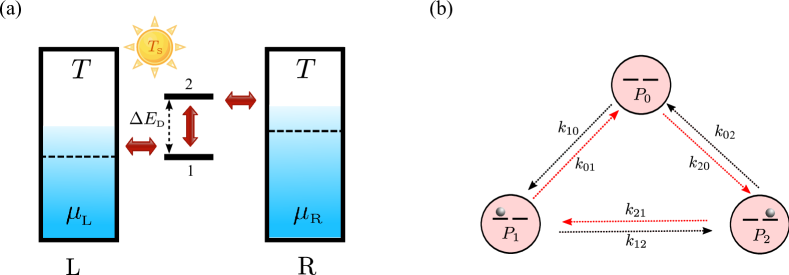
Figure 1: A spinless two-levels, $3$-state model of a solar device that comprises two metal electrodes and a two-level molecule. Levels $1$ and $2$ are coupled to the left and right electrodes, respectively. The molecule can be in states $0=|0,0\rangle$, $1=|1,0\rangle$ and $2=|0,1\rangle$ where $|n_{1},n_{2}\rangle$ is a state with $n_{1}$ electrons in level $1$ and $n_{2}$ electrons in level $2$ (double occupancy is not allowed).

Under conditions that lead to equilibrium at long time, the ratios between these rates are determined by the ambient temperature $T$ , the level energies $E_{1}$, $E_{2}$ and the chemical potential $\mu$ that characterizes electrons in the metal electrodes, and are given by the detailed balance relations

$$\frac{k_{10}}{k_{01}} =e^{-\beta(E_{1}-\mu)}\,;\quad\frac{k_{21}}{k_{12}}=e^{-\beta(E_{2}-E_{1})}\,;\quad\frac{k_{20}}{k_{02}}=e^{-\beta(E_{2}-\mu)}\,,$$ (2)

where $\beta=1/k_{\rm\scriptscriptstyle B}T$ is the inverse thermal energy and $k_{\rm\scriptscriptstyle B}$ is the Boltzmann constant. Note that the rates $k_{21}$ and $k_{12}$ can originate from radiative transition (thermal radiation) as well as non-radiative processes, both characterized by the ambient temperature $T$. At equilibrium all fluxes vanish, $J_{ji}=k_{ji}P_{i}^{\rm eq}-k_{ij}P_{j}^{\rm eq}$, where $P_{j}$ is the probability that the system is in state $j$. A cyclical network of this property is characterized by the identity

$$\frac{k_{02}k_{21}k_{10}}{k_{20}k_{12}k_{01}}=1$$ (3)

that is satisfied by the ratio between forward and backward rates in a reaction loop, provided that these rates sustain a state of zero loop current.

In an operating photovoltaic cell the system is taken out of this equilibrium in two ways: (a) Radiative pumping (an damping) is affected on the $1$-$2$ transition. In standard models of photovoltaic cells this pumping is represented by an effective temperature $T_{\rm\scriptscriptstyle S}=1/k_{\rm\scriptscriptstyle B}\beta_{\rm\scriptscriptstyle S}$ (“sun temperature”not (a)). With the coupling scheme (1) this leads to electron current from the left to the right electrode, however this short circuit current does not perform any useful work unless (b) an opposing voltage bias $V=\Delta\mu/e$ is set between the two electrodes ($\Delta\mu$ is the corresponding chemical potential difference) so that the photocurrent works against this bias. The kinetic rates now satisfy

$$\frac{k_{10}}{k_{01}} =e^{-\beta(E_{1}-\mu)}\,;\quad\frac{k_{21}}{k_{12}}=e^{-\beta_{\rm\scriptscriptstyle S}(E_{2}-E_{1})}\,;\quad\frac{k_{20}}{k_{02}}=e^{-\beta(E_{2}-\mu)}\,,$$ (4)

where $\mu_{2}=\mu_{1}+\Delta\mu$ and $T=1/k_{\rm\scriptscriptstyle B}\beta$ is the ambient temperature. At steady state, the current $J$ is the same on all segments of the graph of Fig. 1(b)

$$J =k_{10}P_{0}-k_{01}P_{1}=k_{21}P_{1}-k_{12}P_{2}=k_{02}P_{2}-k_{20}P_{0}$$ (5)

The open circuit (OC) voltage is the bias for which this current vanish. The existence of such a state again implies that these rates satisfy Eq. (3). Equations (3) and (4) then lead to

$$\frac{\Delta\mu^{\rm OC}}{E_{2}-E_{1}} =1-\frac{T}{T_{\rm\scriptscriptstyle S}}$$ (6)

Viewed as the zero current limit of the efficiency $J\Delta\mu/[J(E_{2}-E_{1})]$ (ratio between the work per unit time, $\dot{W}=J\Delta\mu$ extracted from the device and the heat per unit time, $\dot{Q}=(E_{2}-E_{1})J$ absorbed from sun), Eq. (6) simply identifies the efficiency in this reversible (zero current) limit as the Carnot efficiency. Remarkably, this result does not depend on the relative alignment of the molecular levels with respect to the electrodes Fermi levels. It does rely on the assumption that all input “sun heat” enters at the resonance energy $E_{2}-E_{1}$, and identifies the inability of this system to efficiently extract energy from photons of different energies as an important source of loss.

This simple example demonstrates the use of kinetic schemes that incorporate rate information in the analysis of photovoltaic device performance, as well as its relationship to thermodynamics. Naturally, Carnot efficiency is realized in the OC limit. In the following two sections we apply a similar analysis to a simple model of bulk heterojunction organic photovoltaic (BHJ-OPV) cell, where essential internal losses leads to a maximum efficiency that is lower than the Carnot result.

III BHJ-OPV Model

The BHJ-OPV cell model considered here is comprised of two effective sites $l=\rm D,\,A$ representing the donor (D) and the acceptor (A) molecules, in contact with two electrodes, $L$ and $R$ (see Fig. 2). Each of the sites is described as a two-state system with energy levels $\varepsilon_{\rm\scriptscriptstyle D1},\varepsilon_{\rm\scriptscriptstyle D2}$) and ($\varepsilon_{\rm\scriptscriptstyle A1},\varepsilon_{\rm\scriptscriptstyle A2}$) corresponding to the highest occupied and lowest unoccupied molecular orbitals (HOMO, LUMO) levels of the donor and acceptor species, respectively. The electrodes are represented by free-electron reservoirs at chemical potentials $\mu_{K}$ ($K=L,R$) that are set to $\varepsilon_{\rm\scriptscriptstyle F}=\varepsilon_{\rm\scriptscriptstyle D1}+\Delta E_{\rm\scriptscriptstyle D}/2$ ($\Delta E_{\rm\scriptscriptstyle D}=\varepsilon_{\rm\scriptscriptstyle D2}-\varepsilon_{\rm\scriptscriptstyle D1}$) in the zero-bias junction. The electrochemical potential difference corresponds to a bias The electrochemical potential difference corresponds to a bias voltage $U=(\mu_{\rm\scriptscriptstyle R}-\mu_{\rm\scriptscriptstyle L})/|e|$ where $|e|$ is the electron charge. In what follows we use the notation $\Delta E_{l}=\varepsilon_{l2}-\varepsilon_{l1}$ ($l=\rm D,\,A$), for the energy differences that represent the donor and acceptor band gaps, and refer to $\Delta\varepsilon=\varepsilon_{\rm\scriptscriptstyle D2}-\varepsilon_{\rm\scriptscriptstyle A2}$ as the interface or donor-acceptor LUMO-LUMO gap.not (b) The different system states are described by occupation numbers $n_{\rm\scriptscriptstyle K_{j}}=0,1$, where $K=D,A$ and $j=1,2$.

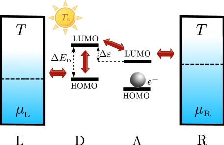
Figure 2: Schematic representation of energetics in BHJ solar cells. The system consists of a donor and acceptor, each characterized by their HOMO and LUMO levels.

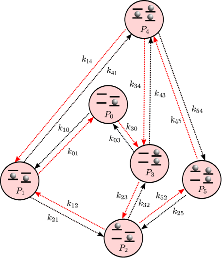
Figure 3: (Network representation of the underlying master equation associated with the six accessible microstates. The graph is composed of six vertices (shown as circles). The interconnected vertices represent the probabilities $P_{N}$ to find the system in a microstate $N$ ($N=0,...,5$) and the edges connecting some pairs of vertices stand for transitions between the states. The edges are drawn as arrows that indicate transitions with rate $k_{N^{\prime}\,N}=k_{N^{\prime}\leftarrow N}$ from a state (vertex) $N$ to $N^{\prime}$.

To further assign realistic contents to this model we introduce the restrictions $n_{\rm\scriptscriptstyle D1}n_{\rm\scriptscriptstyle D2}=0$ (i.e., the donor cannot be double occupied) and $n_{\rm\scriptscriptstyle A1}=1$. The second condition implies that the acceptor can only receive (and subsequently release) an additional electron. Because of this restriction, the energy $\varepsilon_{\rm\scriptscriptstyle A2}$ can be taken as the corresponding single electron energy given that level $A_{1}$ is occupied. The resulting microscopic description then consists of six states with respect to the occupations $(n_{\rm\scriptscriptstyle D1},\,n_{\rm\scriptscriptstyle D2},\,n_{\rm\scriptscriptstyle A1},\,n_{\rm\scriptscriptstyle A2})$, that we denote by the integers $N=0,\,...,\,5$, (see Fig. 3). Within this six-state representation, the probability to find the system in state $N$ is denoted by $P_{N}$. The system dynamics is modeled by a master equation accounting for the time evolution of the probabilities $P_{N}(t)$ ($N=0,\,...,\,5$) fulfilling normalization $\sum_{N}P_{N}(t)=1$ at all times (for details, see Ref. Einax et al., 2011). The steady state is evaluated by setting $dP_{N}(t)/dt=0$.

In what follows, we assume that the transition rates $k_{N^{\prime}\,N}=k_{N^{\prime}\leftarrow N}$ from state $N$ to state $N^{\prime}$ obey (local) detailed balance condition, i. e. their ratios are given by $k_{N^{\prime}\,N}/k_{N\,N^{\prime}}=\exp(-\beta_{\nu}\Delta E_{N^{\prime}\,N})$, where $\Delta E_{N^{\prime}\,N}=E_{N^{\prime}}-E_{N}$. Note that in general $\Delta E_{N^{\prime}\,N}$ is determined by intrinsic energy differences as well as external driving forces.Einax et al. (2010a) $\beta_{\nu}=1/k_{\rm\scriptscriptstyle B}T_{\nu}$ is the inverse thermal energy associated with a thermal bath at temperature $T_{\nu}$. As in the $2$-level example addressed in Section II, some of the rates processes are governed by the ambient temperature $T$, while others reflect external driving force. In the present model the latter are the $1\rightleftharpoons 2$ and $4\rightleftharpoons 5$ transitions, which are governed by the effective temperature $T_{\rm\scriptscriptstyle eff}$ defined below.

Because the heterojunction architecture entails an intrinsic energy loss associated with the exciton dissociation, the energetics is determined by both the interfacial gap energy $\Delta\varepsilon$ and the exciton binding energy. In what follows we will define the exciton binding energy $V_{\rm\scriptscriptstyle C}$ as the difference between the energy needed to move the electron from donor upper level $D2$ to the acceptor level $A2$, and the same energy evaluated in the fictitious case in which the Coulombic electron-hole interaction is disregarded. It is important to note the difference between this many body energy and the essentially single electron energies $\varepsilon_{\rm\scriptscriptstyle K_{j}}$, $K=D,A$, $j=1,2$. The latter are properties of the single electron levels depicted in Fig. 2, and their differences enter in evaluating the transition energies between the corresponding levels. In contrast, $V_{\rm\scriptscriptstyle C}$ is a property of a transition between states $2$ and $3$ (see Fig. 3) and does not enter any other transition energy. (This assumes, as we do here, that the exciton binding energy is fully realized in this transition, i. e., that the corresponding electron-hole Coulomb attraction does not extend beyond the nearest neighbor $D$-$A$ distance). Thus $E_{3}-E_{2}=\varepsilon_{\rm\scriptscriptstyle A2}-\varepsilon_{\rm\scriptscriptstyle D2}+V_{\rm\scriptscriptstyle C}$, however (for example) $E_{1}-E_{0}=E_{4}-E_{3}=\varepsilon_{\rm\scriptscriptstyle D1}-\mu_{L}$ and $E_{3}-E_{0}=E_{5}-E_{2}=\varepsilon_{\rm\scriptscriptstyle A2}-\mu_{R}$ do not depend on $V_{\rm\scriptscriptstyle C}$. With this understanding, the energy differences $\Delta E_{N^{\prime}\,N}=E_{N^{\prime}}-E_{N}$ between any two molecular states depicted in Fig. 3 can be written and used as described below.

IV Thermodynamic efficiency limit from a cycle representations

The six system states shown in Fig. 3 are connected by rate processes, forming a graph in which the states are represented by nodes while the rate processes corresponds to the links between them. This graph can be decomposed into cycles, as detailed in Table 1.

Let us focus on the fundamental cycle associated with the path $C_{1}$: $P_{0}\rightarrow P_{1}\rightarrow P_{2}\rightarrow P_{3}\rightarrow P_{0}$. This cycle represents the photovoltaic operation of the considered minimal model for a BHJ-OPV solar cell. In the “forward direction” it starts with electron transfer from the left electrode into level $D1$ ($P_{0}\rightarrow P_{1}$), followed by light induced promotion of the electron to level $D2$ ($P_{1}\rightarrow P_{2}$), exciton dissociation, that is electron transfer from $D2$ to $A2$ ($P_{2}\rightarrow P_{3}$) and, finally, transfer of the excess electron on level $A2$ of the acceptor to the right electrode. These processes are of course accompanied by their reverse counterparts. The energies associated with these transitions are $\Delta E_{10}=\varepsilon_{\rm\scriptscriptstyle D1}-\mu_{\rm\scriptscriptstyle L}$, $\Delta E_{21}=\varepsilon_{\rm\scriptscriptstyle D2}-\varepsilon_{\rm\scriptscriptstyle D1}=\Delta E_{D}$, $\Delta E_{32}=\varepsilon_{\rm\scriptscriptstyle A2}-\varepsilon_{\rm\scriptscriptstyle D2}+V_{\rm\scriptscriptstyle C}=V_{\rm\scriptscriptstyle C}-\Delta\varepsilon$, and $\Delta E_{03}=\mu_{\rm\scriptscriptstyle R}-\varepsilon_{\rm\scriptscriptstyle A2}$. The corresponding rates satisfy detailed balance conditions that are determined by these energies and the corresponding temperatures. The processes $0\rightleftharpoons 1$, $2\rightleftharpoons 3$, and $3\rightleftharpoons 0$ are governed by the ambient temperature $T$. Consequently

$$\frac{k_{10}}{k_{01}} =e^{-(\varepsilon_{\rm\scriptscriptstyle D1}-\mu_{\rm\scriptscriptstyle L})/k_{\rm\scriptscriptstyle B}T}\,,$$ (7)

$$\frac{k_{32}}{k_{23}} =e^{-(V_{\rm\scriptscriptstyle C}-\Delta\varepsilon)/k_{\rm\scriptscriptstyle B}T}\,,$$ (8)

and

$$\frac{k_{03}}{k_{30}} =e^{-(\mu_{\rm\scriptscriptstyle R}-{\varepsilon}_{\rm\scriptscriptstyle A2})/k_{\rm\scriptscriptstyle B}T}\,.$$ (9)

Consider now the photoinduced $1\rightleftharpoons 2$ process. In general, both the forward and reverse transitions are associated with radiative and non-radiative excitation and recombination

$$k_{12} =k_{12}^{\rm R}+k_{12}^{\rm NR}\,;\quad k_{21}=k_{21}^{\rm R}+k_{21}^{\rm NR}\,.$$ (10)

The radiative rates are photoinduced by sunlight and satisfy a detailed balance condition associated with the sun temperature $T_{\rm\scriptscriptstyle S}$, while the non- radiative rates are determined by interaction with the environment and obey a detailed balance relation governed by the ambient temperature

$$\frac{k_{21}^{R}}{k_{12}^{R}} =e^{-\Delta E_{\rm\scriptscriptstyle D}/k_{\rm\scriptscriptstyle B}T_{\rm\scriptscriptstyle S}}\,;\quad\frac{k_{21}^{NR}}{k_{12}^{NR}}=e^{-\Delta E_{\rm\scriptscriptstyle D}/k_{\rm\scriptscriptstyle B}T}\,.$$ (11)

Table 1: Cycles associated with the network of the systems states given in Fig. 2.

CYCLE	PATH
C1	$P_{0}\rightarrow P_{1}\rightarrow P_{2}\rightarrow P_{3}\rightarrow P_{0}$
C2	$P_{0}\rightarrow P_{1}\rightarrow P_{4}\rightarrow P_{5}\rightarrow P_{2}\rightarrow P_{3}\rightarrow P_{0}$
C3	$P_{1}\rightarrow P_{2}\rightarrow P_{3}\rightarrow P_{4}\rightarrow P_{1}$
$C_{4}$	$P_{2}\rightarrow P_{3}\rightarrow P_{4}\rightarrow P_{5}\rightarrow P_{2}$
C5	$P_{1}\rightarrow P_{2}\rightarrow P_{5}\rightarrow P_{4}\rightarrow P_{1}$
C6	$P_{0}\rightarrow P_{1}\rightarrow P_{4}\rightarrow P_{3}\rightarrow P_{0}$

Consequently

$$\frac{k_{21}}{k_{12}} \equiv\frac{k_{21}^{\rm R}+k_{21}^{\rm NR}}{k_{12}^{\rm R}+k_{12}^{\rm NR}}=e^{-\Delta E_{\rm\scriptscriptstyle D}/k_{\rm\scriptscriptstyle B}T_{\rm\scriptscriptstyle eff}}\,,$$ (12)

where the effective temperature $T_{\rm\scriptscriptstyle eff}$ is defined by

$$T_{\rm\scriptscriptstyle eff} =\frac{\Delta E_{\rm\scriptscriptstyle D}}{k_{\rm\scriptscriptstyle B}}\frac{1}{\ln\big{[}\frac{k_{12}^{\rm R}+k_{12}^{\rm NR}}{k_{21}^{\rm R}+k_{21}^{\rm NR}}\big{]}}\,.$$ (13)

In the absence of radiationless loss ($k_{12}^{\rm NR}=k_{21}^{\rm NR}=0$) $T_{\rm\scriptscriptstyle eff}=T_{\rm\scriptscriptstyle S}$. In the presence of such loss, Eq. (13) implies that (since $T<T_{\rm\scriptscriptstyle S}$) $T_{\rm\scriptscriptstyle eff}<T_{\rm\scriptscriptstyle S}$ . Note that the absolute magnitude of $T_{\rm\scriptscriptstyle eff}$ is determined not only by the temperatures $T$ and $T_{\rm\scriptscriptstyle eff}$ but also by the kinetic rates themselves: faster non-radiative recombination implies lower effective temperature.

Next, suppose that the cycle $C_{1}$ represents the entire energy conversion device. Consider the ratio of products of forward and backward, rates, $k_{10}k_{21}k_{32}k_{03}$ and $k_{01}k_{12}k_{23}k_{30}$ in cycle $C_{1}$. From Eqs. (7)-(9) and (12) we get

$$\frac{k_{10}k_{21}k_{32}k_{03}}{k_{01}k_{12}k_{23}k_{30}} =e^{-(\Delta\mu-\Delta E_{\rm\scriptscriptstyle D}+V_{\rm\scriptscriptstyle C})/k_{\rm\scriptscriptstyle B}T}e^{-\Delta E_{\rm\scriptscriptstyle D}/k_{\rm\scriptscriptstyle B}T_{\rm\scriptscriptstyle eff}}\equiv e^{-A(C_{1})/k_{\rm\scriptscriptstyle B}T}\,,$$ (14)

where $\Delta\mu=\mu_{\rm\scriptscriptstyle R}-\mu_{\rm\scriptscriptstyle L}$. The quantity $A(C_{1})$ defined by (14) is the affinity of the cycle $C_{1}$. It can be recast in the form

$$A(C_{1}) =\frac{\Delta\mu+V_{\rm\scriptscriptstyle C}-\Delta E_{\rm\scriptscriptstyle D}\eta_{\rm\scriptscriptstyle eff}^{\rm\scriptscriptstyle C}}{k_{\rm\scriptscriptstyle B}T}\,,$$ (15)

where

$$\eta_{\rm\scriptscriptstyle eff}^{\rm\scriptscriptstyle C} =1-\frac{T}{T_{\rm\scriptscriptstyle eff}}$$ (16)

is the Carnot efficiency of a reversible machine operating between temperatures $T$ and $T_{\rm\scriptscriptstyle eff}$. As discussed in Sec. II, the cycle affinity vanishes when the cycle carries no current. In this reversible case Eq. (15) yields

$$\frac{\Delta\mu^{\rm OC}}{\Delta E_{\rm\scriptscriptstyle D}} =\eta_{\rm\scriptscriptstyle eff}^{\rm\scriptscriptstyle C}-\frac{V_{\rm\scriptscriptstyle C}}{\Delta E_{\rm\scriptscriptstyle D}}\,.$$ (17)

As discussed in Sec. II [see Eq. (6)], the left hand side of this equation represents the energy conversion efficiency of our device. When $T_{\rm\scriptscriptstyle eff}=T_{\rm\scriptscriptstyle S}$ (i. e. in the absence of nonradiative recombination) and $V_{\rm\scriptscriptstyle C}=0$ (vanishing exciton binding energy), this device operates, in this open circuit limit, at the Carnot efficiency associated with the sun temperature. Equation (17) shows explicitly the two sources of efficiency reduction in this reversible (open voltage) situation: The presence of non-radiative recombination which renders an effective temperature lower than $T_{\rm\scriptscriptstyle S}$ and the exciton binding energy that needs to be overcome during the operation at the cost of useful work.

The result (17) is an expression for the maximal efficiency of a device operating along cycle $C_{1}$. However, it is easily checked that the same condition for vanishing affinity is obtained for any of the cycles in Table 1 that contains the exciton dissociation ($2\rightleftharpoons 3$) step, namely cycles $C_{1}$,$C_{2}$,$C_{3}$, and $C_{4}$. (To verify this note that $k_{43}/k_{34}=k_{10}/k_{01}$, and $k_{14}/k_{41}=k_{25}/k_{52}=k_{03}/k_{30}$). Furthermore, for the both cycles $C_{5}$ and $C_{6}$ we find $A(C_{5})=A(C_{6})=0$. Therefore the result (17) is valid for the original $6$-state system depicted in Figs. 2 and 3. Note that in the absence of non-radiative recombination, Eq. (17) becomes

$$\frac{\Delta\mu^{\rm OC}}{\Delta E_{\rm\scriptscriptstyle D}} =\eta^{\rm\scriptscriptstyle C}-\frac{V_{\rm\scriptscriptstyle C}}{\Delta E_{\rm\scriptscriptstyle D}}\,;\quad\eta^{\rm\scriptscriptstyle C}=1-\frac{T}{T_{\rm\scriptscriptstyle S}}\,,$$ (18)

which is compatible with the result of Ref. Giebink et al., 2011.

Equations (13), (16), and (17) provide a simple and transparent view of the sources of OC voltage reduction and reversible efficiency loss in BHJ-OPV cells. We have checked this result by solving the underlying master equation given inEinax et al. (2010a). To this end we have adapted the energetics and the transitions rates used in this previously work:Einax et al. (2010a) $\mu_{\rm\scriptscriptstyle L}=0.0\,\rm eV$, $\mu_{\rm\scriptscriptstyle R}=\mu_{\rm\scriptscriptstyle L}+\Delta\mu$, $\varepsilon_{\rm\scriptscriptstyle D1}=-0.1\,\rm eV$, $\varepsilon_{\rm\scriptscriptstyle D2}=1.4\,\rm eV$, $\varepsilon_{\rm\scriptscriptstyle A2}=1.15\,\rm eV$ and $V_{\rm\scriptscriptstyle C}=0.15\,\rm eV$, and have set the temperatures to $T=300\rm K$ and $T_{\rm\scriptscriptstyle S}=6000\rm K$ so the Carnot efficiency is $\eta^{\rm\scriptscriptstyle C}=0.95$. For simplicity we neglect radiationless losses on the donor.not (c) The numerical calculation gives the open circuit voltage $\Delta\mu^{\rm OC}=1.275$  eV, which agrees exactly with that value predicted by Eq. (18), i. e., $\Delta\mu^{\rm OC}=0.95\Delta E_{\rm\scriptscriptstyle D}-0.15\,{\rm eV}=1.275$  eV. For $V_{\rm\scriptscriptstyle C}=0.15$  eV, the maximal achievable thermodynamic efficiency is $\eta^{\rm\scriptscriptstyle th}=0.85$.

V Conclusion and Perspectives

We have presented a novel concept for performance analysis of photovoltaic cells and have applied it to the simplest $2$-level device model as well as a generic model for an organic photovoltaic cell. The starting point is the modelling of the energy conversion process by a set of kinetic (master) equations with rate coefficients that incorporate the system energy level structure as well as the relevant energetic, thermal and optical constraints and driving forces. Further analysis is facilitated by describing the resulting master equation as a graph in which the rates are represented by edges that link between vortices representing states. This makes it possible to exploit the decomposition of the network into cycles to get better insight on the interrelations between the physical fluxes. Such a kinetic scheme can be used to analyze the system performance at and away from equilibrium, however in this paper we have focused on open circuit (OC) situations, in particular the simplest subclass of those in which all internal currents, therefore all cycle affinities, vanish. The performance of such systems does not depends on individual rates, only on ratios between backward and forward rates that are determined by detailed balance conditions. For the $2$-level/$3$-state device model of references 30 and 32 this analysis yields the Carnot value for the maximum OC efficiency. A similar calculation for a generic model of a bulk heterojunction organic photovoltaic (BHJ-OPV) cell that incorporates the exciton dissociation energy as well as non-radiative recombination in the donor-subsystem leads to a maximum OC efficiency and OC voltage that are lower than the limiting Carnot value. For example, with our choice of (reasonable) parameters the maximum available efficiency is found to be $0.85$ , which $\sim 10\%$ lower than the corresponding Carnot value ($\sim 0.95$). This approach can be generalized in several ways. Operation under finite overall current can be analyzed to yield efficiency at maximum power.Einax and Nitzan Even under OC conditions, loss due to the presence of cycles with nonvanishing currents can be encountered in more complex models and should be accounted for. Finally, extending such approach to the quantum-mechanical regime may be of interest. These will be subjects of future efforts.