Gravitational quantum effects on power spectra and spectral indices with higher-order corrections

Abstract

The uniform asymptotic approximation method provides a powerful, systematically-improved, and error-controlled approach to construct accurate analytical approximate solutions of mode functions of perturbations of the Friedmann-Robertson-Walker universe, designed especially for the cases where the relativistic linear dispersion relation is modified after gravitational quantum effects are taken into account. These include models from string/M-Theory, loop quantum cosmology and Hořava-Lifshitz quantum gravity. In this paper, we extend our previous studies of the first-order approximations to high orders for the cases where the modified dispersion relation (linear or nonlinear) has only one-turning point (or zero). We obtain the general expressions for the power spectra and spectral indices of both scalar and tensor perturbations up to the third-order, at which the error bounds are $\lesssim 0.15\%$. As an application of these formulas, we calculate the power spectra and spectral indices in the slow-roll inflation with a nonlinear power-law dispersion relation. To check the consistency of our formulas, we further restrict ourselves to the relativistic case, and calculate the corresponding power spectra, spectral indices and runnings to the second-order. Then, we compare our results with the ones obtained by the Green function method, and show explicitly that the results obtained by these two different methods are consistent within the allowed errors.

I Introduction

The cosmological inflation not only solves most problems of the standard big bang cosmology, but also provides the simplest and most elegant mechanism to produce the primordial density perturbations and primordial gravitational waves (PGWs) Guth ; InfGR . The former grows to produce the observed large-scale structure of the universe, and meanwhile creates the cosmic microwave background (CMB) temperature anisotropy, which was already detected by various CMB observations COBE ; WMAP ; PLANCK and galaxy surveys GSs . PGWs, on the other hand, produce not only a temperature anisotropy, but also a distinguishable signature in CMB polarization - the B mode polarization, which has been observed recently by the ground based BICEP2 experiment BICEP2 . These observations have unprecedented precisions in the measurement of the power spectra and spectral indices, and together with the forthcoming ones, provide unique opportunities for us to get deep insight on the physics of the very early universe. More important, they could provide an unique window to explore gravitational quantum effects, which otherwise cannot be studied in the near future by any man-made lab experiments.

On the other hand, as is well known, the inflationary scenario is conceptually incomplete in serval respects Brandenberger1999 ; Martin2001 . For example, in most of the inflation models, the energy scale of quantum fluctuations, which relate to the present observations, were not far from the Planck scale at the beginning of inflation. Thus, questions immediately arise as to whether the usual predictions of the scenario in the framework of semi-classical approximations still remain robust due to the ignorance of gravitational quantum physics at such high energy and, more interestingly, whether they could leave imprints for future observations. Further problems of inflationary scenario include the existence of the initial singularities sing , and the particular initial conditions Burgess . Yet, a large tensor-to-scalar ratio $r\sim 0.16$, measured recently by BICEP2 BICEP2 , leads to the so-called Planckian excursion of the inflaton field, which makes the effective theory of inflation questionable ZW14 .

All the problems mentioned above are closely related to the high energy physics that the usual classical general relativity (GR) and effective field theory of inflation are known to break down. It is widely expected that new physics in this regime — quantum theory of gravity, will provide a complete description of the early universe. Although such a theory has not been properly formulated, gravitational quantum effects on inflation have already been studied extensively by various approaches. See, for example, Brandenberger1999 ; Martin2001 ; Ashtekar ; Burgess ; ZW14 ; eff ; Brandenberger2013CQG , and references therein. In most of these considerations, both the scalar and tensor perturbations produced during the inflationary epoch are governed by the equation

$$\mu_{k}^{\prime\prime}(\eta)+\left(\omega_{k}^{2}(\eta)-\frac{z^{\prime\prime}(\eta)}{z(\eta)}\right)\mu_{k}(\eta)=0,$$ (1.1)

where $\mu_{k}(\eta)$ denotes the mode function, a prime the differentiation with respect to the conformal time $\eta$. $k$ is the comoving wavenumber, and $z(\eta)$ depends on the background and the types of perturbations (scalar and tensor). The modified dispersion relation $\omega_{k}^{2}(\eta)$ depends on both the specified quantum gravity models and scenarios of inflation. For example, in the Hořava-Lifshitz quantum gravity Horava , $\omega_{k}^{2}(\eta)$ takes the form HL

$$\omega_{k}^{2}(\eta)=k^{2}\left[1-\hat{b}_{1}\left(\frac{k}{aM_{*}}\right)^{2}+\hat{b}_{2}\left(\frac{k}{aM_{*}}\right)^{4}\right],$$ (1.2)

where $M_{*}$ is the relevant energy scale of the trans-Planckian physics, $a=a(\eta)$ is the scalar factor of the background universe, $\hat{b}_{1}$ and $\hat{b}_{2}$ are dimensionless constants. When $\hat{b}_{1}=0=\hat{b}_{2}$, it reduces to that of GR,

$$\omega_{k}^{2}(\eta)=k^{2}.$$ (1.3)

The dispersion relation is also modified in models of string/M-theory. For example, in the DBI inflation DBI it takes the form

$$\omega_{k}^{2}(\eta)=c_{s}^{2}(\eta)k^{2},$$ (1.4)

where $c_{s}(\eta)$ is the effective sound speed. Interestingly, $c_{s}^{2}(\eta)$ could be very close to zero in the far UV regime Martin_K1 ; Martin_K2 .

In the framework of loop quantum cosmology, $\omega_{k}^{2}(\eta)$ is also modified. For example, with the holonomy corrections holonomy ; loop_corrections , $\omega_{k}^{2}(\eta)$ becomes

$$\omega_{k}^{2}(\eta)=\left(1-\frac{2\rho(\eta)}{\rho_{c}}\right)k^{2},$$ (1.5)

where $\rho(\eta)$ denotes the energy density of the universe, and $\rho_{c}$ the critical energy density at which a big bounce occurs, whereby the classical initial singularity of the universe is removed. On the other hand, the inverse-volume corrections loop_corrections ; Bojowald2008b lead to

$$\omega_{k}^{2}(\eta)=\begin{cases}s^{2}(\eta)k^{2},&\mbox{ scalar},\cr(1+2\hat{\alpha}_{0}\delta_{\text{PL}})k^{2},&\mbox{tensor},\cr\end{cases}$$ (1.6)

with

$$s^{2}(\eta)=1+\left[\frac{\sigma\nu_{0}}{3}\left(\frac{\sigma}{6}+1\right)+\frac{\hat{\alpha}_{0}}{2}\left(5-\frac{\sigma}{3}\right)\right]\delta_{PL}(\eta),$$

where $\hat{\alpha}_{0},\;\nu_{0},\;\text{and}\;\sigma$ encode the specific features of the model.

In addition to the above mentioned models, mode functions with other modified dispersion relations have also been studied phenomenologically to mimic quantum gravitational effects in the very early universe dissipative ; lorentzbrane .

To study these quantum effects, a critical step is to solve Eq.(1.1) analytically for the mode function $\mu_{k}(\eta)$, and then extract information from it, including the power spectra, spectral indices and runnings. Such studies are very challenging, as the problem becomes mathematically very much involved, and meanwhile the treatment needs to be very accurate, in order to match with the observational data of current and forthcoming experiments. Currently, in most of the analytical treatments of the mode functions with modified dispersion relations the corresponding errors are unknown, and frequently are by far beyond the required accuracy by observations. This yields a big gap between the treatments of these rich phenomenological models of the very early universe and the high precision observational data.

The attempt to close this gap was initiated by Habib et al uniformPRL , in which the uniform asymptotic approximation was first introduced to inflationary cosmology. However, they considered only the relativistic case, in which the dispersion relation is the standard linear one given by Eq.(1.3). In addition, the mode function was constructed only to the first-order approximation, for which the error bounds in general are $\lesssim 15\%$ . Clearly, this is not accurate enough to match with the accuracy of the observational data. Moreover, their results cannot be applied to the cases with nonlinear dispersion relations, mentioned above.

In order to account for the quantum effects, recently we generalized the uniform asymptotic approximation method of Habib et al uniformPRL ; uniformPRD to the cases with non-linear dispersion relations, where multiple and high-order turning points are allowed Zhu2 . From such obtained approximate solutions of the mode functions, we calculated the power spectra and the corresponding spectral indices of scalar and tensor perturbations to the first-order approximation. However, as pointed out above, in general the error bounds are only $\lesssim 15\%$, although in some cases further improvement can be done, as in the relativistic case uniformPRD .

To match with the accuracy of the current and forthcoming observations, we need at least to consider the slow-roll approximation to the second-order, which requires considerations of the high-order approximations even in the framework of the uniform asymptotic approximations. This is precisely what we are going to do in this paper. In particular, by working out explicitly the high-order uniform asymptotic approximations, we obtain the accurate analytical solutions of the mode function at an arbitrary high-order for the case where only one single turning point exists. We construct explicitly the error bounds associated with the approximations order by order. With the accurate analytical solutions of the mode functions, we obtain the general expressions of the power spectra and spectral indices up to the third-order.

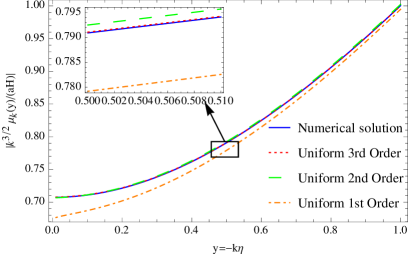
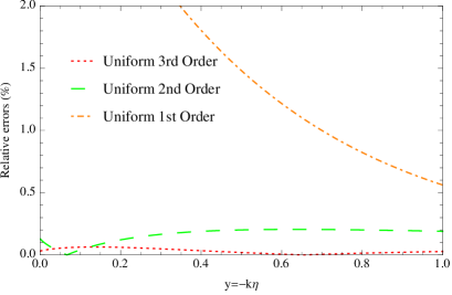
As an application of the developed formulas, we calculate explicitly the power spectra and spectral indices of scalar and tensor perturbations with the modified dispersion relation given by Eq.(1.2) in the slow-roll inflation approximation. To test the consistency of our formulas, we further restrict ourselves to the relativistic case ($\hat{b}_{1}=\hat{b}_{2}=0$), in which the power spectra, spectral indices, and the corresponding runnings of spectral indices have been calculated to the second-order by using the Green function method green1 ; green2 . We compare the results obtained by these two different methods, and show that they are essentially the same within the allowed errors. In this case, we also compare our results order by order with the numerical (exact) results for the evolution of the mode functions, and the results are illustrated in Fig.1, from which one can see that our analytical results to the second- and third-order approximations are extremely closed to the exact results.

Specifically, the paper is organized as follows. In Sec. II, we present a brief review of the uniform asymptotic approximation method. In the case where there is only one turning point, the mode function is expanded in terms of $1/\lambda$ to an arbitrarily high order, in which the error bounds are given in each of the orders. In Sec. III we obtain the general expressions of the power spectra and spectral indices to the third-order from the analytical approximate mode function given in Sec. II, after first matching it with the initial conditions. In Sec. IV, we apply the general expressions obtained in Sec. III to the inflationary model with the nonlinear power-law dispersion relation (1.2), and calculate the power spectra, and spectral indices in the slow-roll inflation. In Sec. V, we consider the GR limit of the power spectra and spectral indices, and also calculate the runnings of the spectral indices and the tensor-to-scalar ratio. Furthermore, we compare the power spectra and spectral indices with those obtained by the Green function method, and show that the two sets of expressions are essentially identical within the allowed errors. Our main conclusions are summarized in Sec. VI. Four appendices, A-D, are also included, in which various detailed mathematical calculations are presented.

II The uniform asymptotic approximations

In this section, we present a brief introduction to the uniform asymptotic approximation method for the cases where the dispersion relation has only a single turning point.

Following refs. uniformPRL ; Olver1974 ; ZWCKS ; Zhu2 , by introducing a dimensionless variable $y=-k\eta$, let us first write the equation of the mode function in the form

$$\frac{d^{2}\mu_{k}(y)}{dy^{2}}=\left[\lambda^{2}\hat{g}(y)+q(y)\right]\mu_{k}(y).$$ (2.1)

In the above the parameter $\lambda$ is used to trace the order of the uniform approximations, and $\lambda^{2}\hat{g}(y)=g(y)$. Usually $\lambda$ is supposed to be large, and it also can be absorbed into $g(y)$ thus when we turn to determine the final results, we can set $\lambda=1$ for the sake of simplification. From Eq.(1.1) we find that

$$\lambda^{2}\hat{g}(y)+q(y)\equiv-\frac{1}{k^{2}}\left(\omega^{2}_{k}(\eta)-\frac{z^{\prime\prime}(\eta)}{z(\eta)}\right).$$ (2.2)

In most of the cases, $\hat{g}(y)$ and $q(y)$ have two poles (singularities): one is at $y=0^{+}$ and the other is at $y=+\infty$. As we discussed in Zhu2 (see also uniformPRL ; Olver1974 ), if these two poles are both second-order or higher, one has to choose

$$q(y)=-\frac{1}{4y^{2}},$$ (2.3)

for the convergence of the error control functions. In this paper we shall restrict our discussions to this choice. In addition, the function $\hat{g}(y)$ can vanish at various points, which are called turning points or zeros, and the approximate solution of the mode function $\mu_{k}(y)$ depends on the behavior of $\hat{g}(y)$ and $q(y)$ near the turning points.

To proceed further, let us first introduce the Liouville transformations with two new variables $U(\xi)$ and $\xi$ via the relations,

$$U(\xi) = \chi^{1/4}\mu_{k}(y),\;\;\;\xi^{\prime 2}=\frac{|g(y)|}{f^{(1)}(\xi)^{2}},$$ (2.4)

where $\chi\equiv\xi^{\prime 2},\;\xi^{\prime}=d\xi/dy$, and

$$f(\xi) = \int^{y}\sqrt{|g(y)|}dy,\;\;\;f^{(1)}(\xi)=\frac{df(\xi)}{d\xi}.$$ (2.5)

Note that $\chi$ must be regular and not vanish in the intervals of interest. Consequently, $f(\xi)$ must be chosen so that $f^{(1)}(\xi)$ has zeros and singularities of the same type as that of $g(y)$. As shown below, such requirement plays an essential role in determining the approximate solutions. In terms of $U$ and $\xi$, Eq.(2.1) takes the form

$$\frac{d^{2}U}{d\xi^{2}} = \left[\pm f^{(1)}(\xi)^{2}+\psi(\xi)\right]U,$$ (2.6)

where

$$\psi(\xi)=\frac{q(y)}{\chi}-\chi^{-3/4}\frac{d^{2}(\chi^{-1/4})}{dy^{2}},$$ (2.7)

and the signs “$\pm$” correspond to $g(y)>0$ and $g(y)<0$, respectively. Considering $\psi(\xi)=0$ as the first-order approximation, one can choose $f^{(1)}(\xi)$ so that the first-order approximation can be as close to the exact solution as possible with the guidelines of the error functions constructed below, and then solve it in terms of known functions. Clearly, such a choice sensitively depends on the behavior of the functions $g(y)$ and $q(y)$ near the poles and turning points.

In this paper, we consider only the case in which $\hat{g}(y)$ has only one single turning point $\bar{y}_{0}$ (for $\hat{g}(y)$ having several different turning points or one multiple-turning point, see Zhu2 ), i.e., $\hat{g}(\bar{y}_{0})=0$. In this case we can choose

$$f^{(1)}(\xi)=\pm\xi,$$ (2.8)

here $\xi=\xi(y)$ is a monotone decreasing function, and $\pm$ correspond to $\hat{g}(y)\geq 0$ and $\hat{g}(y)\leq 0$, respectively. Following Olver Olver1974 , the general solution of Eq.(2.6) can be written as

$$U(\xi) = \alpha_{0}\Bigg{[}\text{Ai}(\lambda^{2/3}\xi)\sum_{s=0}^{n}\frac{A_{s}(\xi)}{\lambda^{2s}}$$

$$~{}~{}~{}~{}~{}~{}~{}+\frac{\text{Ai}^{\prime}(\lambda^{2/3}\xi)}{\lambda^{4/3}}\sum_{s=0}^{n-1}\frac{B_{s}(\xi)}{\lambda^{2s}}+\epsilon_{3}^{(2n+1)}\Bigg{]}$$

$$+\beta_{0}\Bigg{[}\text{Bi}(\lambda^{2/3}\xi)\sum_{s=0}^{n}\frac{A_{s}(\xi)}{\lambda^{2s}}$$

$$~{}~{}~{}~{}~{}~{}~{}~{}+\frac{\text{Bi}^{\prime}(\lambda^{2/3}\xi)}{\lambda^{4/3}}\sum_{s=0}^{n-1}\frac{B_{s}(\xi)}{\lambda^{2s}}+\epsilon_{4}^{(2n+1)}\Bigg{]},$$

where $\text{Ai}(x)$ and $\text{Bi}(x)$ represent the Airy functions, $\epsilon_{3}^{(2n+1)}$ and $\epsilon_{4}^{(2n+1)}$ are errors of the approximate solution, and

$$A_{0}(\xi)=1,\;\;$$

$$B_{s}(\xi)=\frac{\pm 1}{2(\pm\xi)^{1/2}}\int_{0}^{\xi}\{\psi(v)A_{s}(v)-A^{\prime\prime}_{s}(v)\}\frac{dv}{(\pm v)^{1/2}},$$

$$A_{s+1}(\xi)=-\frac{1}{2}B^{\prime}_{s}(\xi)+\frac{1}{2}\int\psi(v)B_{s}(v)dv,$$

where $\pm$ correspond to $\xi\geq 0$ and $\xi\leq 0$, respectively. The error bounds of $\epsilon_{3}^{(2n+1)}$ and $\epsilon_{4}^{(2n+1)}$ can be expressed as

$$\frac{\epsilon_{3}^{(2n+1)}}{M(\lambda^{2/3}\xi)},\;\;\frac{\partial\epsilon_{3}^{(2n+1)}/\partial\xi}{\lambda^{2/3}N(\lambda^{2/3}\xi)}$$

$$~{}~{}~{}~{}~{}\leq 2E^{-1}(\lambda^{2/3}\xi)\exp{\left[\frac{2\kappa_{0}\mathscr{V}_{\alpha,\xi}(|\xi^{1/2}|B_{0})}{\lambda}\right]}$$

$$~{}~{}~{}~{}~{}~{}~{}~{}~{}~{}~{}\times\frac{\mathscr{V}_{\alpha,\xi}(|\xi^{1/2}|B_{n})}{\lambda^{2n+1}},$$

$$\frac{\epsilon_{4}^{(2n+1)}}{M(\lambda^{2/3}\xi)},\;\;\frac{\partial\epsilon_{4}^{(2n+1)}/\partial\xi}{\lambda^{2/3}N(\lambda^{2/3}\xi)}$$

$$~{}~{}~{}~{}~{}\leq 2E(\lambda^{2/3}\xi)\exp{\left[\frac{2\kappa_{0}\mathscr{V}_{\xi,\beta}(|\xi^{1/2}|B_{0})}{\lambda}\right]}$$

$$~{}~{}~{}~{}~{}~{}~{}~{}~{}~{}~{}\times\frac{\mathscr{V}_{\xi,\beta}(|\xi^{1/2}|B_{n})}{\lambda^{2n+1}},$$ (2.11)

where the definitions of $M(x)$, $N(x)$, $\kappa_{0}$, and $\mathscr{V}_{a,b}(x)$ can be found in Zhu2 .

Having obtained the approximate solution of the mode function $\mu_{k}(y)$, let us compare it with the numerical solution order by order. For the sake of simplification, we consider a linear dispersion relation $\omega_{k}^{2}(\eta)=k^{2}$ and a de-Sitter background, i.e, $\nu=3/2$. In the top panel of Fig.1, we present the numerical (exact) solution, the approximate solution of the first-, second-, and third-orderapproximations, respectively. From this figure one can see clearly that our analytical solutions to the second- and third-order approximations are extremely closed to the exact ones. In practice, our analytical solution of the third-order approximation is not distinguishable to the numerical one. In the low panel of Fig.1, we also display the relative error ($\%$) of the three approximate solutions, in comparing them with the exact solution.

Figure 1: The mode function $|k^{3/2}\mu_{k}(y)/(aH)|$ and the corresponding relative errors of the first- second- and third-order approximations of the uniform asymptotic method presented in this paper as well as that of the numerical (exact) solution. (a) Top panel: the numerical solution (blue solid curve) and the approximate solutions of the third-order (red dotted curve), second-order (green dashed curve), and first-order approximation (orange dot-dashed curve). (b) Low panel: The relative errors of the approximate solutions of the third-order (red dotted curve), second-order (green dashed curve), and first-order approximations (orange dot-dashed curve). In drawing the above figures, we have set $\nu=3/2$, $\omega_{k}^{2}(\eta)=k^{2}$ and the mode function was initially at Bunch-Davies vacuum.

III Power spectra and spectral indices up to the third-order

With the approximate solution given in the last section, now let us begin to calculate the power spectra and spectral indices from the approximate solution. We assume that the universe was initially at the adiabatic vacuum,

$$\lim_{y\to 0^{+}}\frac{1}{\sqrt{2\omega_{k}(\eta)}}e^{-i\int\omega_{k}(\eta)d\eta},$$ (3.1)

and one needs to match this initial state with the approximate solution (II). However, the approximate solution (II) involves many high-order terms, which are complicated and not easy to handle. In order to simplify them, we first study their behavior in the limit $y\rightarrow+\infty$. Let us start with the $B_{0}(\xi)$ term in Eq.(II), which satisfies

$$B_{0}(\xi)=-\frac{1}{2\sqrt{-\xi}}\int_{0}^{\xi}\frac{\psi(v)}{\sqrt{-v}}dv=-\frac{\mathscr{H}(\xi)}{2\sqrt{-\xi}},$$ (3.2)

where $\mathscr{H}(\xi)\equiv\int_{0}^{\xi}dv\psi(v)/|v|^{1/2}$ is the associated error control function of the approximate solution (II), and in the above we have used $A_{0}(\xi)=1$. The error control function $\mathscr{H}(\xi)$ is well behaved around the turning point $\bar{y}_{0}$ and converges when $y\to+\infty$. As a result, we have

$$\lim_{y\rightarrow+\infty}B_{0}(\xi)=-\frac{\mathscr{H}(-\infty)}{2\sqrt{-\xi}}.$$ (3.3)

Then, let us turn to $A_{1}$, which is

$$A_{1}(\xi)=-\frac{1}{2}B_{0}^{\prime}(\xi)+\frac{1}{2}\int_{0}^{\xi}\psi(v)B_{0}(v)dv.$$ (3.4)

In the limit $y\rightarrow+\infty$, $B_{0}^{\prime}(\xi)$ vanishes, and we find

$$\lim_{y\to+\infty}A_{1}(\xi) = -\frac{1}{2}\int_{0}^{\xi}\frac{\psi(v)}{\sqrt{-v}}\left[\frac{1}{2}\int_{0}^{v}\frac{\psi(u)}{\sqrt{-u}}du\right]dv$$ (3.5)

$$= -\frac{1}{2}\left[\frac{\mathscr{H}(-\infty)}{2}\right]^{2}.$$

Note that in the above we have used the formula

$$n!\int_{\xi_{0}}^{\xi}f(\xi_{n})\int_{\xi_{0}}^{\xi_{n}}f(\xi_{n-1})\cdots\int_{\xi_{0}}^{\xi_{2}}f(\xi_{1})d\xi_{1}d\xi_{2}\cdots d\xi_{n}$$

$$~{}~{}~{}~{}~{}~{}~{}~{}~{}~{}~{}~{}~{}~{}~{}~{}~{}~{}~{}~{}~{}~{}~{}~{}~{}~{}~{}~{}~{}~{}=\left[\int_{\xi_{0}}^{\xi}f(v)dv\right]^{n}.$$ (3.6)

Thus, up to the third-order, we have

$$A_{0}(\xi)+\frac{A_{1}(\xi)}{\lambda^{2}} = 1-\frac{1}{2\lambda^{2}}\left[\frac{\mathscr{H}(-\infty)}{2}\right]^{2}+\mathcal{O}\left(\frac{1}{\lambda^{3}}\right),\;\;\;\;\;$$

$$\frac{B_{0}(\xi)}{\lambda} = -\frac{1}{\sqrt{-\xi}}\frac{\mathscr{H}(-\infty)}{2\lambda}+\mathcal{O}\left(\frac{1}{\lambda^{3}}\right).$$ (3.7)

Thus, using the asymptotic form of Airy functions in the limit $\xi\to-\infty$, and comparing the solution $\mu_{k}(y)$ with the initial state, we obtain

$$\alpha_{0}=\sqrt{\frac{\pi}{2k}}\frac{1}{(A_{0}+A_{1}/\lambda^{2})-i\sqrt{-\xi}B_{0}/\lambda},$$

$$\beta_{0}=i\sqrt{\frac{\pi}{2k}}\frac{1}{(A_{0}+A_{1}/\lambda^{2})-i\sqrt{-\xi}B_{0}/\lambda},$$ (3.8)

where we have

$$(A_{0}+A_{1}/\lambda^{2})-i\sqrt{-\xi}B_{0}/\lambda=(1+\mathcal{O}(1/\lambda^{3}))e^{i\theta},$$ (3.9)

here $\theta$ is an irrelevant phase factor, and without loss of generality, we can set $\theta=0$. Thus, we finally get

$$\alpha_{0}=\sqrt{\frac{\pi}{2k}},\;\;\;\beta_{0}=i\sqrt{\frac{\pi}{2k}}.$$ (3.10)

After determining the coefficients $\alpha_{0}$ and $\beta_{0}$, we can calculate the power spectra of the perturbations. As $y\rightarrow 0$, only the growing mode is relevant, thus we have

$$\mu_{k}(y) \simeq \beta_{0}\left(\frac{\xi}{\hat{g}(y)}\right)^{1/4}\Bigg{[}\text{Bi}(\lambda^{2/3}\xi)\sum_{s=0}^{+\infty}\frac{B_{s}(\xi)}{\lambda^{2s}}$$ (3.11)

$$\;\;\;\;\;\;\;\;\;\;\;\;+\frac{\lambda^{2/3}\text{Bi}^{\prime}(\lambda^{2/3}\xi)}{\lambda^{2}}\sum_{s=0}^{+\infty}\frac{B_{s}(\xi)}{\lambda^{2s}}\Bigg{]}.\;\;\;\;\;\;\;\;$$

In order to calculate the power spectra to higher order, let us first consider the $B_{0}(\xi)$ term, which satisfies

$$\lim_{y\to 0}B_{0}(\xi)=\frac{1}{2\xi^{1/2}}\int_{0}^{\xi}\frac{\psi(v)}{v^{1/2}}dv=\frac{\mathscr{H}(+\infty)}{2\xi^{1/2}}.$$ (3.12)

In the above we had used the relation $\xi^{1/2}d\xi=-\sqrt{\hat{g}}dy$. Knowing the $B_{0}$ term, we can get the $A_{1}$ term, which is

$$\lim_{y\to 0}A_{1}(\xi) = \frac{1}{4}\int_{0}^{\xi}\frac{\psi(v)}{v^{1/2}}\int_{0}^{v}\frac{\psi(u)}{u^{1/2}}dudv$$ (3.13)

$$= \frac{1}{2}\left[\frac{\mathscr{H}(+\infty)}{2}\right]^{2}.$$

Thus up to the third order and considering the asymptotic forms of the Airy functions in the limit $\xi\rightarrow+\infty$, we find

$$\lim_{y\rightarrow 0}\mu_{k}(y) = \frac{\beta_{0}e^{\frac{2}{3}\lambda\xi^{2/3}}}{\lambda^{1/6}\hat{g}^{1/4}\pi^{1/2}}\Bigg{[}1+\frac{\mathscr{H}(+\infty)}{2\lambda}+\frac{\mathscr{H}(+\infty)^{2}}{8\lambda^{2}}$$ (3.14)

$$~{}~{}~{}~{}~{}~{}~{}~{}~{}~{}~{}~{}~{}~{}~{}~{}~{}~{}~{}~{}~{}~{}~{}~{}+\mathcal{O}(1/\lambda^{3})\Bigg{]}.$$

Then, the power spectra can be calculated, and is given by

$$\Delta^{2}(k) \equiv \frac{k^{3}}{2\pi^{2}}\left|\frac{\mu_{k}(y)}{z}\right|^{2}_{y\to 0^{+}}$$

$$\simeq \frac{k^{2}}{4\pi^{2}}\frac{-k\eta}{z^{2}(\eta)\nu(\eta)}\exp\left(2\int_{y}^{\bar{y}_{0}}\sqrt{\hat{g}(\hat{y})}d\hat{y}\right)$$

$$\;\times\left[1+\frac{\mathscr{H}(+\infty)}{\lambda}+\frac{\mathscr{H}^{2}(+\infty)}{2\lambda^{2}}+\mathcal{O}(1/\lambda^{3})\right].$$

It should be noted that the general expressions of the power spectra have been obtained in uniformPRL up to the second-order, while in the above expressions the last term in the square brackets represents the third-order approximation.

From the power spectra presented above, one can get the general expression of the spectral indices, which now is given by

$$n-1 \equiv \frac{d\ln\Delta^{2}(k)}{d\ln k}$$ (3.16)

$$\simeq 3+2\int_{y}^{\bar{y}_{0}}\frac{d\hat{y}}{\sqrt{\hat{g}(\hat{y})}}+\frac{1}{\lambda}\frac{d\mathscr{H}(+\infty)}{d\ln k}$$

$$+\mathcal{O}\left(\frac{1}{\lambda^{3}}\right),$$

and the last term in the above expression represents the second- and third-order approximations.

It should be noted that the above results represent the most general expressions of the power spectra and spectral indices of perturbations for the case that has only one-turning point. In the following we shall apply these expressions to some particular backgrounds and dispersion relations, and calculate the power spectra and spectral indices.

IV Power spectra and spectral indices with nonlinear power-law dispersion relation in the slow roll inflation

In this section, as an application of the general results obtained in the last section, let us consider a specific case where the conventional linear dispersion relation is replaced by the nonlinear one given in Eq.(1.2). For simplification, in this section and hereafter we set $\lambda=1$ and thus we have $\hat{g}(y)=g(y)$. In order to get a healthy ultraviolet limit one requires $\hat{b}_{2}>0$. It is convenient to write the nonlinear dispersion relation as

$$\omega_{k}^{2}(\eta)=k^{2}\left(1-b_{1}\epsilon_{*}^{2}y^{2}+b_{2}\epsilon_{*}^{4}y^{4}\right),$$ (4.1)

where $\epsilon_{*}\equiv H/M_{*}$ with $H$ representing the Hubble parameter, which is slowly varying during inflation, and $b_{1}\equiv\hat{b}_{1}/(a\eta H)^{2}$, $b_{2}\equiv\hat{b}_{2}/(a\eta H)^{4}$. Then, it is easy to find that

$$g(y)=\frac{\nu^{2}}{y^{2}}-1+b_{1}\epsilon_{*}^{2}y^{2}-b_{2}\epsilon_{*}^{4}y^{4},$$ (4.2)

where we had used the relation

$$\frac{z^{\prime\prime}}{z}\equiv\frac{\nu^{2}(\eta)-1/4}{\eta^{2}}.$$ (4.3)

Now, let us determine explicitly the power spectra from Eq.(III). We first need to consider the integral of $\sqrt{g(y)}$. However, with the form (4.2), the explicit form of the integral usually cannot be worked out explicitly. Thus, we adopt the expansion given in Zhu2 ,

$$\sqrt{g(y)} \simeq \sqrt{\frac{y_{0}^{2}}{y^{2}}-1}\Bigg{\{}1-\frac{b_{2}}{2}(y^{2}+y_{0}^{2})\epsilon_{*}^{2}$$ (4.4)

$$-\left[\frac{b_{1}^{2}}{8}(y^{2}+y_{0}^{2})^{2}-\frac{b_{2}}{2}(y^{4}+y^{2}y_{0}^{2}+y_{0}^{4})\right]\epsilon_{*}^{4}$$

$$\;\;+\mathcal{O}(\epsilon_{*}^{4})\Bigg{\}}.$$

Note that to derive the above we had assumed that $\epsilon_{*}$ is small. It should be noted that unlike in Zhu2 where we had treated all the parameters as constant in the first-order slow roll approximation, here in order to go beyond the first-order, we have to treat all the parameters $y_{0},\;\epsilon_{*},\;b_{1},\;\text{and}\;b_{2}$ as time-dependent.

Even with the above expansion, the integral still cannot be done explicitly, if the explicit form of $y_{0}(\eta),\;b_{1}(\eta),\;b_{2}(\eta),\;\text{and}\;\epsilon_{*}(\eta)$ are not known. As discussed in uniformPRL ; uniformPRD , the integrand in (III) has a square-root singularity at the turning point, i.e., at the upper integral limit. At the lower limit where $y$ goes to zero, the integrand vanishes linearly. Thus one expects the main contribution to the integral to arise from the upper limit. With this in mind, one can expand all the slowly varying quantities, for example $y_{0}(\eta)$, around the turning point $y(\eta_{0})=y_{0}(\eta_{0})$ as

$$y_{0}(\eta)\simeq\bar{y}_{0}+\frac{dy_{0}}{d\eta}\Big{|}_{\eta_{0}}(\eta-\eta_{0})+\frac{1}{2}\frac{d^{2}y_{0}}{d\eta^{2}}\Big{|}_{\eta_{0}}(\eta-\eta_{0})^{2},$$

where $\bar{y}_{0}=-k\eta_{0}$ represents the turning point, and in the above we only expanded $y_{0}(\eta)$ to the second-order. With this kind of expansions we can specify all of the quantities $y_{0}(\eta),\;b_{1}(\eta),\;b_{2}(\eta),\;\epsilon_{*}(\eta)$, and then calculate the power spectra, spectral indices, and runnings of the indices to the desired accuracy. However, if one considers the slow roll inflation, as pointed out in uniformPRD , the above expansions and the slow roll expansion are not independent. On the other hand, by using the slow roll expansion given in Appendix A, one can see that the higher derivative terms which have been ignored in (IV) also contain second-order terms in the slow roll approximation. This means that the final results shall loose some accuracy at the second-order slow roll approximation. Here we should point out that the above analysis is only valid if one makes use of the slow roll approximation.

An alternative expansion of the above quantities was used in Martin_K1 ; Martin_K2 , in which $y_{0}(\eta)$ is given by

$$y_{0}(\eta) \simeq \bar{y}_{0}+\frac{dy_{0}}{d\ln(-\eta)}\Big{|}_{\eta_{0}}\ln\left(\frac{y}{\bar{y}_{0}}\right)$$ (4.6)

$$+\frac{1}{2}\frac{d^{2}y_{0}}{d\ln^{2}(-\eta)}\Big{|}_{\eta_{0}}\ln^{2}\left(\frac{y}{\bar{y}_{0}}\right).$$

From the slow roll expansion of high-order derivatives in $y_{0}(\eta)$, one can see that

$$\frac{d^{n}y_{0}}{d\ln^{n}(-\eta)}\sim\mathcal{O}(\epsilon^{n+1})+\mathcal{O}(\epsilon^{n})\mathcal{O}(\epsilon_{*}^{2}),$$ (4.7)

here $\epsilon$ represents the first-order slow-roll quantities. Thus, if one only considers the power spectra up to the second-order, the higher terms beyond the second-order in terms of the slow roll parameters can be safely ignored. With this kind of expansions, we can obtain the explicit expressions of $\sqrt{g(y)}$, the integral of $\sqrt{g(y)}$, and also the error control function $\mathscr{H}(+\infty)$. We present these results in appendices A and B. In Appendices C and D, we present all the slow roll expansions of $\nu(\eta)$, $y_{0}(\eta)$, $H(\eta)$, $b_{1}(\eta)$, etc. In the following we shall use these results to calculate the power spectra and spectral indices of both scalar and tensor perturbations.

First, let us consider the scalar perturbations, for which we have

$$z_{s}(\eta)=\sqrt{2\epsilon(\eta)}a(\eta).$$ (4.8)

Then, we expand the scalar spectrum (III) in terms of slow-roll parameters ($\epsilon,\;\delta_{1},\;\delta_{2},\;\delta_{3}$, etc, which are all defined in appendix C) and $\epsilon_{*}$, and find

$$\Delta_{s}^{2}(k) \simeq \frac{181\bar{H}^{2}}{72e^{3}\pi^{2}\bar{\epsilon}}\Bigg{\{}1+\frac{909}{724}\hat{b}_{1}\bar{\epsilon}_{*}^{2}-\frac{81\left(763\hat{b}_{1}^{2}-1752\hat{b}_{2}\right)\bar{\epsilon}_{*}^{4}}{28960}$$ (4.9)

$$+\left[4\ln 2-\frac{630}{181}+\left(\frac{2727}{362}\ln 2-\frac{5769}{724}\right)\hat{b}_{1}\bar{\epsilon}_{*}^{2}-\frac{27\left(2\hat{b}_{1}^{2}(8348+11445\ln 2)+\hat{b}_{2}(14591-52560\ln 2)\right)}{36200}\bar{\epsilon}_{*}^{4}\right]\bar{\epsilon}$$

$$+\left[\ln 4-\frac{134}{181}+\frac{3(157+606\ln 2)\hat{b}_{1}}{724}\bar{\epsilon}_{*}^{2}-\frac{27\left(\hat{b}_{1}^{2}(1909+4578\ln 2)-2\hat{b}_{2}(3163+5256\ln 2)\right)}{28960}\bar{\epsilon}_{*}^{4}\right]\bar{\delta}_{1}$$

$$+\Bigg{[}\frac{\pi^{2}}{3}-\frac{6367}{1629}+4\ln^{2}2-\frac{536\ln 2}{181}\Bigg{]}\bar{\epsilon}^{2}+\Bigg{[}\frac{5\pi^{2}}{12}-\frac{9374}{1629}+3\ln^{2}2-\frac{40\ln 2}{181}\Bigg{]}\bar{\epsilon}\bar{\delta}_{1}$$

$$+\Bigg{[}-\frac{\pi^{2}}{12}-\frac{26}{1629}+3\ln^{2}2-\frac{402\ln 2}{181}\Bigg{]}\bar{\delta}_{1}^{2}+\Bigg{[}\frac{543\pi^{2}-688-1629\ln^{2}4+4824\ln 2}{6516}\Bigg{]}\bar{\delta}_{2}\Bigg{\}}.$$

The corresponding scalar spectral index can be calculated from Eq.(3.16), which is given by

$$n_{s} = 1-4\bar{\epsilon}-2\bar{\delta}_{1}-\frac{5\hat{b}_{1}}{2}\bar{\epsilon}_{*}^{2}\bar{\epsilon}+\frac{9}{10}\left(13\hat{b}_{1}^{2}-22\hat{b}_{2}\right)\bar{\epsilon}\bar{\epsilon}_{*}^{4}$$ (4.10)

$$+\Bigg{[}8\ln 2-\frac{296}{27}-\frac{23}{2}\bar{\epsilon}_{*}^{2}\hat{b}_{1}+\frac{3}{200}\bar{\epsilon}_{*}^{4}\left(-1607\hat{b}_{1}^{2}+1560\ln 2\hat{b}_{1}^{2}+3068\hat{b}_{2}+1410\ln 2\hat{b}_{2}\right)\Bigg{]}\bar{\epsilon}^{2}$$

$$+\Bigg{[}10\ln 2-\frac{262}{27}-\frac{3\bar{\epsilon}_{*}^{4}}{800}\left(11977\hat{b}_{1}^{2}+6240\ln 2\hat{b}_{1}^{2}-10918\hat{b}_{2}-26760\ln 2\hat{b}_{2}\right)+\bar{\epsilon}_{*}^{2}\left(5\ln 2\hat{b}_{2}-\frac{53\hat{b}_{1}}{4}\right)\Bigg{]}\bar{\epsilon}\bar{\delta}_{1}$$

$$+\Bigg{[}\left(\frac{20}{27}-\ln 4\right)\Bigg{]}\bar{\delta}_{1}^{2}+\Bigg{[}\bar{\epsilon}_{*}^{4}\left(\frac{153\hat{b}_{2}}{16}-\frac{171\hat{b}_{1}^{2}}{32}\right)+\frac{19}{12}\epsilon_{*}^{2}\hat{b}_{1}+\left(\ln 4-\frac{20}{27}\right)\Bigg{]}\bar{\delta}_{2}$$

$$+\Bigg{[}\frac{4\pi^{2}}{3}-\frac{1204}{27}-8\ln 2\ln 4+\frac{700\ln^{2}4}{27}\Bigg{]}\bar{\epsilon}^{3}+\Bigg{[}\frac{31\pi^{2}}{12}-\frac{3293}{54}-31\ln^{2}2+\frac{2240\ln 2}{27}\Bigg{]}\bar{\epsilon}^{2}\bar{\delta}_{1}$$

$$+\Bigg{[}\frac{\pi^{2}}{4}-\frac{15}{2}-3\ln^{2}2+\frac{56\ln 2}{9}\Bigg{]}\bar{\epsilon}\bar{\delta}^{2}+\Bigg{[}\frac{7\pi^{2}}{12}-\frac{91}{18}-7\ln^{2}2+\frac{356\ln 2}{27}\Bigg{]}\bar{\epsilon}\bar{\delta}_{2}$$

$$+\Bigg{[}\frac{\pi^{2}}{6}-\frac{25}{81}-2\ln^{2}2+\frac{40\ln 2}{27}\Bigg{]}\bar{\delta}_{1}^{3}+\Bigg{[}-\frac{\pi^{2}}{4}+\frac{31}{162}+3\ln^{2}2-\frac{20\ln 2}{9}\Bigg{]}\bar{\delta}_{1}\bar{\delta}_{2}$$

$$+\Bigg{[}\frac{\pi^{2}}{12}+\frac{19}{162}-\frac{1}{4}\ln^{2}4+\frac{20\ln 2}{27}\Bigg{]}\bar{\delta}_{3}.$$

Similarly, for the tensor perturbations we have $z_{t}(\eta)=a(\eta)$, and

${\mathrm{\Delta }}_t^2$

References

- (1) A. Guth, Phys. Rev. D23, 348 (1981). See also A.A. Starobinsky, Phys. Lett. B91, 99 (1980); K. Sato, Mon. Not. R. Astron. Soc. 195, 467 (1981).
- (2) D. Baumann, arXiv:0907.5424.
- (3) C. L. Bennett et al., Astrophys. J. 464, L1 (1996); K. M. Gorski et al., ibid., 464, L11 (1996).
- (4) E. Komatsu et al. (WMAP Collaboration), Astrophys. J. Suppl. Ser. 192, 18 (2011); D. Larson et al. (WMAP Collaboration), ibid., 192, 16 (2011).
- (5) P. Ade et al. (PLANCK Collaboration), arXiv:1303.5082.
- (6) D.J. Eisenstein, et al., Astrophys. J. 633, 560 (2005); S. Cole, et al., Mon. Not. Roy. Astron. Soc. 362, 505 (2005); M. Tegmark, et al. Phys. Rev. D74, 123507 (2006); W. J. Percival, et al. Astrophys. J. 657, 51 (2007); Mon. Not. Roy. Astron. Soc. 401, 2148 (2010); E. A. Kazin, et al. ibid., 710, 1444 (2010); F. Beutler, et al. ibid., 416, 3017 (2011); C. Blake, ,ibid., 406, 803 (2010); ibid., 418, 1707 (2011); ibid., 418, 1725 (2011).
- (7) P.A.R. Ade et al. (BICEP2 Collaboration), BICEP2 I: Detection Of B-mode Polarization at Degree Angular Scales, arXiv: 1403.3985.
- (8) R.H. Brandenberger, arXiv:hep-th/9910410.
- (9) J. Martin and R.H. Brandenberger, Phys. Rev. D63, 123501 (2001); ibid., D65, 103514 (2002); ibid., D68, 063513 (2003); J.C. Niemeyer and R. Parentani, ibid., D64, 101301 (2001) (R); L. Bergstorm and U.H. Danielsson, J. High Energy Phys.12, 038 (2002); J. Martin and C. Ringeval, Phys. Rev. D69, 083515 (2004); A. Ashoorioon, A. Kempf, and R.B. Mann, ibid., 71 , 023503 (2005); A. Ashoorioon, J.L. Hovdebo, and R.B. Mann, Nuc. Phys. B727, 63 (2005); R. Easther, W. H. Kinney, and H. Peiris, J. Cosmol. Astropart. Phys. 05 (2005) 009; A. Ashoorioon, D.Chialvab, and U. Danielsson, ibid., 06, 034 (2011); M.G. Jackson and K. Schalm, Phys. Rev. Lett. 108, 111301 (2012).
- (10) A. Borde and A. Vilenkin, Phys. Rev. Lett. 72, 3305 (1994); A. Borde, A.H. Guth, and A. Vilenkin, Phys. Rev. Lett. 90, 151301 (2003).
- (11) C.P. Burgess, M. Cicoli, and F. Quevedo, arXiv: 1306.3512.
- (12) T. Zhu and A. Wang, Phys. REv. D90, 027304 (2014); and references therein.
- (13) A. Ashtekar, arXiv: 1303.4989.
- (14) C.P. Burgess, J.M. Cline, F. Lemieux, and R. Holman, J. High Energy Phys. 02 (2003) 048; C.P. Burgess, J.M. Cline, and R. Holman, J. Cosmol. Astropart. Phys. 10 (2003) 004; N. Kaloper, M, Kleban, A.E. Lawrence, and S. Shenker, Phys. Rev. D 66, 123510 (2002); D. Bini and G. Esposito, Phys. Rev. D89, 084032 (2014).
- (15) R.H. Brandenberger and J. Martin, Class. Quantum. Grav. 30 (2013) 113001.
- (16) P. Hořava, Phys. Rev. D79, 084008 (2009).
- (17) T. Takahashi and J. Soda, Phys. Rev. Lett. 102, 231301 (2009); K. Yamamoto, T. Kobayashi, and G. Nakamura, Phys. Rev. D80, 063514 (2009); A. Wang and R. Maartens, ibid., D 81, 024009 (2010); A. Wang, ibid., D82, 124063 (2010); Y.-Q. Huang and A. Wang, ibid., D86, 103523 (2012); T. Zhu, F.-W. Shu, Q. Wu, and A. Wang, ibid., D 85, 044053 (2012); T. Kobayashi, Y. Urakawa, and M. Yamaguchi, J. Cosmol. Astropart. Phys. 04, 025 (2010); Y.-Q. Huang, A. Wang, and Q. Wu, J. Cosmol. Astropart. Phys.10, 010 (2012); T. Zhu, Y.-Q. Huang, and A. Wang, J. High. Energy. Phys.01, 138 (2013).
- (18) M. Alishahiha, E. Silverstein and D. Tong, Phys. Rev. D 70, 123505 (2004); E. Silverstein and D. Tong, Phys. Rev. D 70 (2004) 103505; C. de Rham and A. J. Tolley, J. Cosmol. Astropart. Phys.1005 (2010) 015; X. Chen, Phys. Rev. D 71 (2005) 063506; X. Chen, J. High. Energy. Phys.08 (2005) 045; X. Chen, J. Cosmol. Astropart. Phys.12 (2008) 009 [arXiv:0807.3191 [hep-th]]; J. E. Lidsey and I. Huston, J. Cosmol. Astropart. Phys.07 (2007) 002.
- (19) L. Lorentz, J. Martin, and C. Ringeval, Phys. Rev. D 78, 083513 (2008).
- (20) J. Martin, C. Ringeval, and V. Vennin, J. Cosmol. Astropart. Phys. 06 (2013) 021.
- (21) T. Cailleteau, J. Mielczarek, A. Barrau and J. Grain, Class. Quantum Grav. 29, 095010 (2012); T. Cailleteau, A. Barrau, F. Vidotto, and J, Grain, Phys. Rev. D 86, 087301 (2012).
- (22) A. Barrau, T. Cailleteau, J. Grain, and J. Mielczarek, arXiv: 1309.6896.
- (23) M. Bojowald and G.M. Hossain, Phys. Rev. D 77, 023508 (2008); M. Bojowald and G. Calcagni, J. Cosmol. Astropart. Phys.03 (2011) 032; M. Bojowald, G. Calcagni, and S. Tsujikawa, Phys. Rev. Lett. 107, 211302 (2011).
- (24) J. Adamek, D. Campo, and J.C. Niemeyer, Phys. Rev. D 78, 103507 (2008).
- (25) M.V. Libanov and V.A. Rubakov, Phys. Rev. D 72, 123503 (2005).
- (26) S. Habib, K. Heitmann, G. Jungman, and C. Molina-Paris, Phys. Rev. Lett. 89, 281301 (2002); S. Habib, A. Heinen, K. Heitmann, G. Jungman, and C. Molina-Paris, Phys. Rev. D70, 083507 (2004).
- (27) S. Habib, A.Heinen, K. Heitmann, and G. Jungman, Phys. Rev. D 71, 043518 (2005).
- (28) T. Zhu, A. Wang, G. Cleaver, K. Kirsten, and Q. Sheng, Phys. Rev. D.89, 043507 (2014).
- (29) T. Zhu, A. Wang, G. Cleaver, K. Kirsten, and Q. Sheng, arXiv:1308.1104.
- (30) F.W.J. Olver, Asymptotics and Special functions, (AKP Classics, Wellesley, MA 1997).
- (31) E.D. Stewart and J.-O. Gong, Phys. Lett. B 510 (2001) 1; J. Choe, J.-O. Gong, and E.D. Stewart, J. Cosmol. Astropart. Phys.07 (2004) 012.
- (32) J.-O. Gong, Class. Quantum Grav.21 (2004) 5555.
- (33) J. Martin and D.J. Schwarz, Phys. Rev. D.67, 083512 (2003); R. Casadio, F. Finelli, M. Luzzi and G. Venturi, Phys. Rev. D 71, 043517 (2005); R. Casadio, F. Finelli, M. Luzzi and G. Venturi, Phys. Lett. B 625 (2005) 1.
- (34) T. Zhu, A. Wang, G. Cleaver, K. Kirsten, and Q. Sheng, in preparation (2014).