On Exactly Marginal Deformations Dual to $B$-Field Moduli of IIB Theory on SE₅

Abstract

The complex dimension of the space of exactly marginal deformations for quiver CFTs dual to IIB theory compactified on $Y^{p,q}$ is known to be generically three. Simple general formulas already exist for two of the exactly marginal directions in the space of couplings, one of which corresponds to the sum of the (inverse squared of) gauge couplings, and the other to the $\beta$-deformation. Here we identify the third exactly marginal direction, which is dual to the modulus $\int_{\mbox{\footnotesize{2-cycle}}}B_{2}$ on the gravity side. This identification leads to a relation between the field theory gauge couplings and the vacuum expectation value of the gravity modulus that we further support by a computation related to the chiral anomaly induced by added fractional branes. We also present a simple algorithm for finding similar exactly marginal directions in any CFT described by brane tiling, and demonstrate it for the quiver CFTs dual to IIB theory compactified on $L^{1,5,2}$ and the Suspended Pinch Point.

1 Introduction

The AdS/CFT correspondence has become one of the main tools for understanding the strong coupling behavior of four dimensional gauge theories. With minimal supersymmetry (eight supercharges in AdS₅/CFT₄, or four supercharges when conformality is broken) gauge theories appearing in the duality exhibit rich enough behavior to be of great interest, yet are sufficiently under computational control that testable non-trivial information about them can be obtained from their gravitational dual. One often arrives at such dual pairs by probing the singular tip of a Calabi-Yau cone with a stack of D3-branes. The geometry dual to the IR theory on the branes is of the form AdS${}_{5}\times$SE₅, with SE₅ the five-dimensional Sasaki-Einstein base of the cone Klebanov:1998 ; Acharya:1999 ; Morrison:1998 .

$Y^{p,q}$ are a countably infinite family of Sasaki-Einstein 5-manifolds that provide interesting supersymmetric compactifications of IIB supergravity with simple quiver gauge theories as CFT duals Gauntlett:2004a ; Gauntlett:2004b ; Martelli:2004 ; Bertolini:2004xf ; Benvenuti:2004 . Since their discovery about a decade ago, these pairs of AdS/CFT duals have been under considerable study and a variety of their aspects, including the operators dual to classical strings Benvenuti:2005 and supersymmetric branes on the gravity side Canoura:2005uz , is by now well understood. In particular, in Herzog:2005 ; Benvenuti:2005a it was realized that the conformal manifold of the quiver gauge theories is (generically) three-complex dimensional, and shortly afterwards all the three gravity moduli dual to the exactly marginal directions were identified Lunin:2005 .

However, on the field theory side, although two of the exactly marginal directions were precisely known (one the $\beta$-deformation and the other the sum of gauge couplings), the identification of the third exactly marginal direction is not yet established.

Another more recent advance in understanding these dual pairs was the determination of the complete shortened spectrum of IIB supergravity on $Y^{p,q}$ in Ardehali:2013a (building on earlier work in Berenstein:2005xa ; Kihara:2005nt ; Eager:2012hx ). The shortened supergravity multiplets are dual to protected superfields that are all identified in the literature (see for instance Eager:2012hx ; Benvenuti:2005 ; Martelli:2008a ; Ardehali:XX ), with one exception: the Betti hyper multiplet in the supergravity spectrum.

The Betti hyper multiplet shows up in the KK spectrum because of the non-trivial second cohomology group of $Y^{p,q}$ Eager:2012hx . The multiplet contains a massless scalar that is the linearized version of the gravity modulus $\int_{\Sigma_{2}}B_{2}$ (by $\Sigma_{2}$ we mean the non-trivial two-cycle in $Y^{p,q}$). This gravity modulus is dual to the third exactly marginal deformation referred to earlier. Therefore identifying the operator dual to the Betti hyper multiplet requires finding the exactly marginal direction mentioned above.

In this paper we obtain a closed formula for the elusive exactly marginal operator of $Y^{p,q}$ quivers by analyzing the NSVZ equations. We adopt, following Imamura:2007 , the viewpoint of brane tiling (see Franco:2006bd ; Kennaway:2007 for nice reviews of brane tilings). The authors of Imamura:2007 realized that finding an exactly marginal deformation of field theories described by brane tiling is equivalent to solving a linear system of difference equations. As we show in section 2, one can solve this system of equations for $Y^{p,q}$ quivers to obtain the desired exactly marginal operator.

We will further point out that for general quivers a similar NSVZ analysis can serve as a starting point for a systematic derivation of protected superfields dual to supergravity Betti hyper multiplets. In particular, for gauge theories described by brane tiling the relevant data can be neatly encoded in a matrix (which, for its close connection to the Konishi anomaly equation, we will call the Konishi matrix of the quiver) with the following two nice properties: 1) left null vectors of the matrix yield exactly marginal directions in the space of field theory couplings; 2) any consistent set of baryonic charge assignments to the matter fields gives a right null vector of the matrix.

The identification of the exactly marginal operator dual to the $B$-field modulus of $Y^{p,q}$ theories (given in (8)) leads to a proposal for a relation between the field theory gauge couplings and vev of the gravity modulus (given in (LABEL:eq:marginalCombination)). To check this proposal we turn to the cascading theories obtained by adding fractional branes to $Y^{p,q}$ geometries, and compare the change that the Reeb vector generates in the gravity modulus, with the change in gauge theory couplings generated by the (anomalous) U(1)_R; this is quite similar to an analysis of the chiral anomaly done in Klebanov:2002 for $T^{1,1}$.

The organization of our paper is as follows. In the next section we review the field theoretical approach for finding exactly marginal operators of a gauge theory described by brane tiling. In particular, we introduce the Konishi matrix of the quivers and show that it efficiently encodes all the data relevant for finding exactly marginal deformations dual to $B$-field moduli. In section 3 we focus on $Y^{p,q}$ quivers and present a general expression for their elusive exactly marginal operator. This leads to a relation between the gauge theory couplings and the gravity modulus that we further support by analyzing cascading $Y^{p,q}$ quivers. In section 4 more quiver theories are studied using the Konishi matrix introduced in section 2, and the subtleties that may arise in cases which are more general than $Y^{p,q}$ are discussed. Section 5 contains a summary of our results along with a few closing remarks. In appendix A we prove the properties of the Konishi matrix stated in section 2, and also point out how the matrix can be thought to arise from Konishi anomaly equations without any reference to NSVZ equations. Appendix B contains the field theoretical computation of the chiral anomaly of cascading $Y^{p,q}$ quivers, and the exactly marginal directions of the Suspended Pinch Point quiver are made explicit in appendix C.

2 Exactly marginal directions in brane tilings

In this section we review the field theoretical approach for finding exactly marginal operators in gauge theories described by brane tiling. Most of the content of this chapter is already well-known to the experts. Our only novel contribution is to introduce the Konishi matrix in subsection 2.2, and demonstrate its efficiency in finding exactly marginal combinations of quiver couplings.

Brane tilings provide efficient descriptions of gauge theories on D3-branes transverse to toric singularities Franco:2006bd ; Franco:2006 . These are quiver theories with $N_{g}$ SU(N) gauge factors with couplings $g_{j}$ and field strength superfields $W_{\alpha j}$, $N_{f}$ chiral matter fields $\Phi_{I}$ in bifundamentals or adjoints of the gauge groups, and $N_{W}$ superpotential terms of the form

$$W_{m}=\pm h_{m}\mathrm{Tr}\prod_{I\in m}\Phi_{I},$$

where the $\pm$ signature reflects the dimer structure of the tiling Franco:2006bd . Hence, $j=1,...,N_{g}$, $I=1,...,N_{f}$, and $m=1,...,N_{W}$.

For all such theories Franco:2006bd

$$N_{g}+N_{W}=N_{f}.$$ (1)

In Imamura:2007 , exactly marginal combinations of gauge and superpotential couplings were investigated from the viewpoint of brane tiling. The authors of Imamura:2007 started with NSVZ relations for the running of canonical gauge and superpotential couplings

$$\begin{split}&\beta_{j}\equiv\mu\frac{\mathrm{d}}{\mathrm{d}\mu}\frac{1}{g_{j}^{2}}=\frac{N/8\pi^{2}}{1-g_{j}^{2}N/8\pi^{2}}\left[3-\frac{1}{2}\sum_{I\in j}(1-\gamma_{I})\right],\\ &\beta_{m}\equiv\mu\frac{\mathrm{d}}{\mathrm{d}\mu}h_{m}=-h_{m}\left[3-\sum_{I\in m}(1+\frac{\gamma_{I}}{2})\right].\end{split}$$

In the above relations, $1+\frac{\gamma_{I}}{2}$ is the conformal dimension of the chiral field $\Phi_{I}$, and $I\in j$ (respectively $I\in m$) means that the chiral field $\Phi_{I}$ is charged under the gauge group with coupling $g_{j}$ (respectively, participates in the superpotential term with coupling $h_{m}$).

Next, by introducing a set of coefficients $S^{a}_{j}$ (which turn out to play an important role in our ensuing discussions) for the gauge couplings, and $S^{k}_{m}$ for the superpotential couplings, linear combinations of the form

$$\sum_{j}\frac{8\pi^{2}S^{a}_{j}}{Ng_{j}^{\prime 2}}-\sum_{m}S^{k}_{m}\log h_{m},$$ (2)

with vanishing beta functions were searched for. Any such linear combination would correspond to an exactly marginal direction in the space of couplings Imamura:2007 ; hence from now on we will occasionally refer to such a set of coefficients $S^{a}_{j},S^{k}_{m}$ as an exactly marginal direction of the field theory. The redefined couplings $\frac{1}{g_{j}^{\prime 2}}=\frac{1}{g_{j}^{2}}-\frac{N}{8\pi^{2}}\log{\frac{1}{g_{j}^{2}}}$, and $\log h_{m}$ (instead of just $h_{m}$) were considered because of their simpler beta functions. Note that $1/{g^{\prime}}^{2}$ differs from the real part of the holomorphic coupling $1/g_{h}^{2}$ by $-\sum_{I\in j}\frac{T(r_{I})}{8\pi^{2}}\log Z_{I}$ Terning:2006 , where $Z_{I}$ denotes the wave-function renormalization of $\Phi_{I}$.

The authors of Imamura:2007 realized that the vanishing of the beta function for such combinations amounts to the following relations between the unknown coefficients $S^{a}_{j}$ and $S^{k}_{m}$

$$\sum_{j\in I}S^{a}_{j}=\sum_{m\in I}S^{k}_{m}\quad\text{for every }I.$$ (3)

The left sum is over the two gauge factors under which $I$ is charged, and the one on the right is over the two superpotential terms in which $I$ participates. It is worth remarking that, although it is not emphasized in Imamura:2007 , the above relation remains true in the presence of adjoints: one only has to count the node with adjoint twice on the LHS of (3). This is essentially because the Dynkin index (which appears in the NSVZ beta function) for the adjoint is twice that of the bifundamental.

To summarize this section so far, the problem of finding exactly marginal deformations of the gauge and superpotential couplings of a CFT described by brane tiling is reduced to finding a set of coefficients ${S^{a}_{j},S^{k}_{m}}$ that solve (3); these yield RG invariant combinations of the form (2). We conjecture that the corresponding exactly marginal operators are

$$\sum_{j}S^{a}_{j}(\mathrm{Tr}W_{j}^{2})-\sum_{m}S^{k}_{m}(\frac{32\pi^{2}}{N}W_{m}).$$ (4)

Evidence for this conjecture will be presented after equation (13), and also in appendix A.

In Imamura:2007 , two sets of solutions to (3) were found for an arbitrary gauge theory described by brane tiling.

• The first solution was $S^{a}_{j}=S^{k}_{m}=1$ for all $j$ and $m$; this direction in the space of couplings corresponds to the sum of the (inverse squared of) gauge couplings, and is dual to the supergravity axion-dilaton.

• The second solution was $S^{a}_{j}=0$ for all $j$, and $S^{k}_{m}=\pm 1$, with the signature depending on the sign of the superpotential term $m$; this is the $\beta$-deformation of the field theory, with Lunin-Maldacena gravity dual Lunin:2005 .
  

In the present paper we are interested in going beyond the two sets of general solutions mentioned above. It is well-known (and we will review shortly) that if the quiver CFTs under study are dual to SE₅ geometries with non-trivial two-cycles,

• there are additional solutions to (3) which describe exactly marginal directions arising from baryonic symmetries in field theory. We will refer to these as B-deformations. These are dual to the B-field moduli on the non-trivial two-cycles.

In particular, $Y^{p,q}$ quivers have one such exactly marginal direction, as we will describe in the next section.

We now explain how such additional exactly marginal directions originate from baryonic symmetries of the field theory.

2.1 Exactly marginal directions and baryonic charge assignments

In this subsection we review the argument of Martelli:2008a demonstrating the appearance of additional exactly marginal directions when global baryonic U(1) symmetries are present.

Recall that one can imagine that the $N_{g}$ SU(N) gauge groups in the IR, started out as U(N) gauge groups in the UV, for D3-branes probing a cone over SE₅. However, all the U(1)’s decouple in the IR: the ‘center of mass’ U(1) decouples as nothing is charged under it; $b_{3}($SE${}_{5})$ (defined as the rank of the third homology group of SE₅) of the massless U(1)’s decouple because their gauge coupling goes to zero in the infrared, but they nevertheless yield non-anomalous global baryonic symmetries in the IR theory; the remaining $N_{g}-b_{3}(\text{SE}_{5})-1$ U(1)’s become massive and yield anomalous baryonic currents in the IR.

We are interested in the $b_{3}($SE${}_{5})$ non-anomalous baryonic symmetries. For each of these, we have a baryonic charge assignment for the chiral fields. The baryonic U(1) charges $Q_{J}$ (with $J=1,...,b_{3}($SE${}_{5})$) must satisfy (see for example Herzog:2003 )

$$\begin{split}\sum_{I\in j}Q_{J}(\Phi_{I})=0\quad&\text{for every node }j,\\ Q_{J}(\Phi_{j_{1}\ j_{2}})+Q_{J}(\Phi_{j_{2}\ j_{3}})+...+Q_{J}(\Phi_{j_{r}\ j_{1}})=0\quad&\text{for every loop}.\end{split}$$ (5)

Note that the nodes and loops referred to in the above relations are the ones in the quiver diagram picture, not in the brane tiling.

Now, as argued in Martelli:2008a , for any $R$-charge assignment $\{R^{\ast}_{I}\}$ to the chiral fields yielding zero beta functions for the couplings, the relations in (5) guarantee that $\{R^{\ast}_{I}+\mu Q_{J}(\Phi_{I})\}$, for any $\mu\in\mathbb{R}$, is another zero of the beta functions. Thus, for each one of the $b_{3}($SE${}_{5})$ baryonic charge assignments to the chiral fields there exists an exactly marginal deformation of the theory. We referred to these as B-deformations. The interested reader can find another field theoretical explanation for the origin of B-deformations in baryonic symmetries from the viewpoint of the Konishi anomaly equation in appendix A.

The gravity analog of the above field theoretical analysis is as follows. Each non-trivial two-cycle in SE₅ yields a massless Betti vector in the supergravity KK spectrum. This massless vector is dual to a conserved baryonic current. On the other hand, the non-trivial two-cycle yields a gravity modulus of the form $\int_{\mbox{\footnotesize{2-cycle}}}B_{2}$. This gravity modulus is dual to an exactly marginal operator. Hence, the one-to-one correspondence between baryonic symmetries and their related exactly marginal deformations.

To summarize, there are $b_{3}($SE${}_{5})+2$ solutions to (3). $b_{3}($SE${}_{5})$ of them correspond to B-deformations, and arise from baryonic symmetries. The remaining two correspond to the $\beta$-deformation and the axion-dilaton; these can be thought to arise from the global U(1)$\times$U(1) flavor symmetry (see the Konishi anomaly discussion in appendix A).

It seems like in general a useful rule of thumb is that additional global symmetries in field theory are responsible for a larger conformal manifold. In such cases as $Y^{p,q}$ quivers, we saw that the global baryonic symmetry dual to the non-trivial two-cycle explains the additional exactly marginal direction. We will come back to this rule of thumb a few times.

2.2 A simple algorithm for toric quivers

In this section, we provide a simple algorithm for finding exactly marginal combinations of the form

$$\sum_{j}\frac{8\pi^{2}S^{a}_{j}}{Ng_{j}^{\prime 2}}-\sum_{m}S^{k}_{m}\log h_{m},$$ (6)

for quiver theories described by brane tiling. This algorithm is an immediate consequence of the work in Imamura:2007 .

The central ingredient of the algorithm is a neatly derivable matrix, $B_{K}$, that we will refer to as the Konishi matrix of the quiver. The columns of $B_{K}$ are labeled by the chiral fields $I=1,...,N_{f}$. The first $N_{g}$ rows of the matrix are labeled by the gauge groups $j=1,...,N_{g}$. The rest of the rows are labeled by the superpotential terms $m=1,...,N_{W}$. Equation (1) implies that $B_{K}$ is an $N_{f}\times N_{f}$ square matrix for quivers described by brane tiling.

The entries of the Konishi matrix are filled, in a rather natural way, as follows. For a row labeled by a gauge group $j$ insert one in column $I$ if $I\in j$ (insert two if $I$ is in the adjoint of the $j$th gauge group), and insert zero otherwise. For a row labeled by a superpotential term $m$ insert $-1$ in column $I$ if $I\in m$, and zero otherwise.

Note that the direction of the bifundamental chiral field does not matter in constructing the Konishi matrix. This is because the Dynkin index appearing in the NSVZ beta function is quadratic in the generators.

Now that we described how to form $B_{K}$, we explain two of its main properties. The proofs can be found in appendix A.

• Every baryonic charge assignment satisfying (5) gives an $N_{f}$ tuple $(Q_{J}(X_{1}),...,Q_{J}(X_{N_{f}}))^{T}$ that is a null vector of $B_{K}$.

• Every marginal direction of the form (6) in the space of couplings gives an $N_{f}$ tuple $(S^{a}_{1},...,S^{a}_{N_{g}},S^{k}_{1},...,S^{k}_{N_{W}})$ that is a left null vector of $B_{K}$.

In other words, baryonic charges form null vectors of $B_{K}$, while exactly marginal combinations give null vectors of $B^{T}_{K}$.

For the exactly marginal directions, the statement goes the other way as well: every null vector of $B^{T}_{K}$ yields an exactly marginal combination of the form (6). However, not every null vector of $B_{K}$ gives a consistent baryonic charge assignment. The reason is that the second condition in (5) is not fully ensured for the null vectors of $B_{K}$; only the loops that appear in the superpotential are taken into account by $B_{K}$. As we explain in appendix A, the remaining relevant data for constraining baryonic charge assignments is contained in the two non-trivial cycles of the torus of brane tiling. In fact, since the $\beta$-deformation and the sum of gauge couplings are two exactly marginal directions that do not correspond to any baryonic symmetries, we did expect that the non-trivial baryonic charge assignments be two fewer than the exactly marginal deformations. The previous statements are made more precise in appendix A.

The question arises: how can we then determine the codimension two subspace of the null space of $B_{K}$ that corresponds to the non-trivial baryonic charge assignments?

The answer follows from the statement Imamura:2007 that $S^{a}_{t(I)}-S^{a}_{h(I)}$ (with a hopefully obvious notation for ‘head’ and ‘tail’ of a chiral field) is a consistent assignment of baryonic charge to $\Phi_{I}$. This charge would be zero for all $\Phi_{I}$ if we take the $S^{a}$ coefficients of the two general solutions corresponding to the $\beta$-deformation (with all $S^{a}$ equal to zero) and the axion-dilaton (with all $S^{a}$ equal); the remaining $b_{3}($SE${}_{5})$ exactly marginal directions are the ones that correspond to non-trivial baryonic charge assignments.

Now, when $b_{3}($SE${}_{5})>1$, there are more than one B-deformations in the field theory, and one would like to be able to put these in a one-to-one correspondence with the non-trivial two-cycles in the dual geometry. This is where the knowledge of baryonic charge assignments corresponding to each two-cycle in the dual geometry becomes necessary. Such charge assignments can be algorithmically derived for toric quivers as explained in Franco:2006 . Then comparing $S^{a}_{t(I)}-S^{a}_{h(I)}$ of the exactly marginal directions with the baryonic charge assignments $Q_{J}(X_{I})$ of the two-cycles yields the correspondence between the exactly marginal deformations and their related non-trivial two-cycles in the dual geometry. An example of this kind will be considered in section 4.

To illustrate the above algorithm we now study exactly marginal directions of the Klebanov-Witten CFT dual to IIB theory on AdS${}_{5}\times T^{1,1}$ Klebanov:1998 . The Konishi matrix for this theory is

$$B_{K}=\begin{pmatrix}1&1&1&1\\ 1&1&1&1\\ -1&-1&-1&-1\\ -1&-1&-1&-1\end{pmatrix}.$$

Recall that the first two rows correspond to the two gauge factors, the last two rows to the superpotential terms, and the columns to the four bifundamental chiral fields.

The left null vectors of the above matrix are $(S^{a}_{1},S^{a}_{2},S^{k}_{1},S^{k}_{2})=(1,1,1,1)$, $(0,0,1,-1)$, and $(1,-1,0,0)$. The first one corresponds to the sum of the gauge couplings, the second one to the $\beta$-deformation, and the third one to the B-deformation (the difference of the gauge couplings). These exactly marginal directions are all well known Klebanov:1998 ; Benvenuti:2005a . In fact, more exactly marginal directions are known for this theory Benvenuti:2005a than the three we mentioned. There exist two extra exactly marginal deformations of the theory that arise from adding mesonic exactly marginal operators to the superpotential that were not present in the superpotential of the original theory. These were called “accidentally marginal” operators in Imamura:2007 . Such accidentally marginal deformations are (except for a few remarks) completely ignored in our paper; we only consider deformations by changing the couplings already present in the original theory. Before moving on, however, we would like to point out that the existence of these extra exactly marginal deformations for the conifold theory is consistent with the rule of thumb we mentioned earlier: a bigger global symmetry group yields a larger conformal manifold. In this case, the bigger symmetry group of the conifold theory (compared to $Y^{p,q}$ quivers) forbids the presence of all the exactly marginal operators in the superpotential, but these extra operators could serve to deform the theory later.

To summarize, we presented an algorithm for finding the coefficients $S^{a}$ and $S^{k}$ related to the marginal directions from the $N_{f}\times N_{f}$ Konishi matrix of the quiver; from knowledge of $S^{a}$ coefficients one can then recover the baryonic charge assignments via $S^{a}_{t(I)}-S^{a}_{h(I)}=Q_{J}(X_{I})$. We should point out that there already exists a simpler algorithm in the literature for finding only the $S^{a}$ coefficients (and thereby, the baryonic charge assignments) from the $N_{g}\times N_{g}$ ‘incidence matrix’ of the quiver (see for example Kennaway:2007 ). The incidence matrix is smaller than the Konishi matrix, and therefore easier to compute with, but it can not yield the exactly marginal directions. The extra information that the Konishi matrix is capable to give us is the coefficients $S^{k}$, which along with $S^{a}$ serve to fully specify the exactly marginal directions. Finally, the reader should note that it is not possible to obtain the “accidentally marginal” directions (which arise from mesonic $R$-charge 2 chiral primaries absent in the superpotential) from the Konishi matrix; finding such deformations would require a separate analysis which is not covered at all in the present paper.

We will illustrate the above algorithm with more explicit examples in section 4.

3 The B-deformation of $Y^{p,q}$ quivers

In this section we find the exactly marginal deformation of $Y^{p,q}$ quivers which is dual to the $B$-field modulus on the gravity side. This is done by directly solving equations (3) for $Y^{p,q}$ quivers; no use of the Konishi matrix is made in this section. Based on our result we then propose a relation between the gauge theory couplings and the vev of the complex $B$ field on the non-trivial two-cycle of $Y^{p,q}$. The proposal is further supported by considering the effect of adding fractional branes to $Y^{p,q}$ geometries.

The superfield version of the exactly marginal operator that we find is dual to the Betti hyper multiplet in the supergravity KK spectrum. This result incidentally completes the identification of the protected operators dual to shortened supergravity KK multiplets on generic $Y^{p,q}$. Therefore, we see it appropriate to start by reviewing the light multiplets of supergravity and their low-dimension dual operators.

3.1 AdS/CFT state-operator correspondence for $Y^{p,q}$

The shortened (protected) spectrum of IIB supergravity on AdS${}_{5}\times Y^{p,q}$ is detailed in Ardehali:2013a . There are nine towers of supermultiplets called Graviton, Gravitino 1–4 and Vector 1–4, each filled with representations of SU(2,2$|$1), that we denote by $\mathcal{D}(E_{0},s_{1},s_{2};r)$. Each bulk multiplet also transforms under a specific representation of the isometry group of $Y^{p,q}$, which is SU(2)${}_{j}\times$U(1)${}_{\alpha}\times$U(1)_R; we label representations of the SU(2) by $j$ and $-j\leq N_{\phi}\leq j$, representations of the U(1)_α by $N_{\alpha}$, and representations of the U(1)_R by $N_{\psi}$. See Ardehali:2013a for the detailed quantization conditions.

Conserved multiplets

We begin the discussion with conserved multiplets in the spectrum. There is one conserved multiplet in the Graviton tower. It contains the massless graviton dual to the boundary stress tensor, and a massless vector dual to the boundary $R$-current.

The Vector 1 tower generically contains four conserved vectors, a $j=1$ triplet with $N_{\psi}=N_{\alpha}=0$ and a $j=0$ singlet with $N_{\psi}=N_{\alpha}=0$; these are dual to the boundary flavor currents, in the triplet of the SU(2) and the singlet of the U(1) of the isometry group of $Y^{p,q}$

$$J_{SU(2)_{j}}^{k}=\sum_{i}\mbox{Tr }U_{i}e^{V_{h(i)}}\sigma^{k}\bar{U_{i}}e^{-V_{t(i)}}+\sum_{i}\mbox{Tr }V_{i}e^{V_{h(i)}}\sigma^{k}\bar{V_{i}}e^{-V_{t(i)}},$$

$$J_{U(1)_{\alpha}}=\sum_{i}\mbox{Tr }V_{i}e^{V_{h(i)}}\bar{V_{i}}e^{-V_{t(i)}}-\sum_{i}\mbox{Tr }Y_{i}e^{V_{h(i)}}\bar{Y_{i}}e^{-V_{t(i)}}+\sum_{i}\mbox{Tr }Z_{i}e^{V_{h(i)}}\bar{Z_{i}}e^{-V_{t(i)}},$$ (7)

where the sums are over the bifundamental chiral superfields ($U_{i},V_{i},Y_{i},Z_{i}$) in the quiver, $\sigma^{k}$ are the Pauli matrices, and $V_{h(i)}$ (or $V_{t(i)}$) in each term is the Lie algebra valued superfield of the gauge factor at the head (or tail) of the corresponding chiral bifundamental. We hasten to remind the reader that $Y^{p,q}$ quivers consist of $2p$ nodes and a number of chiral bifundamentals of doublet type ($U,V$) and singlet type ($Y,Z$); see Figure 1 for an example, or Benvenuti:2004 for a review. The coefficients of the terms on the RHS of (7) reflect the U(1)_α charges of the chiral fields.

In the previous paragraph we emphasized generically, because $Y^{1,0}$ and $Y^{2,0}$ (also known as $T^{1,1}$ and $T^{1,1}/\mathbb{Z}_{2}$ respectively) are exceptional: in these geometries there are six such conserved vector multiplets, half of them in the triplet of one SU(2) and the other half in the triplet of the other SU(2) of their isometry group SU(2)${}_{j}\times$SU(2)${}_{l}\times$U(1)_R.

The other conserved multiplet in the bulk is the Betti-vector multiplet which has zero $R$-charge and is singlet under the isometry group of $Y^{p,q}$. The dual boundary operator is a baryonic superfield of the schematic form Martelli:2008a

$$\begin{split}\mathcal{U^{I}}=&-p\sum_{i}\mbox{Tr }U_{i}e^{V_{h(i)}}\bar{U_{i}}e^{-V_{t(i)}}+q\sum_{i}\mbox{Tr }V_{i}e^{V_{h(i)}}\bar{V_{i}}e^{-V_{t(i)}}\\ &+(p-q)\sum_{i}\mbox{Tr }Y_{i}e^{V_{h(i)}}\bar{Y_{i}}e^{-V_{t(i)}}+(p+q)\sum_{i}\mbox{Tr }Z_{i}e^{V_{h(i)}}\bar{Z_{i}}e^{-V_{t(i)}}.\end{split}$$

There are no more conserved multiplets in the spectrum, unless $p=q=1$, where one has $Y^{1,1}=S^{5}/\mathbb{Z}_{2}$ with enhanced isometry and supersymmetry, hence additional conserved gravitino multiplets.

Chiral multiplets with massless scalar components

We now discuss the bulk chiral multiplets with massless scalar components. These scalars are the duals of marginal single-trace deformations at the linearized level.

First, there is the universal hyper multiplet in the Vector 4 tower (and its CP conjugate in Vector 3), transforming in $\mathcal{D}(3,0,0;2)$ (and $\mathcal{D}(3,0,0;-2)$) of SU(2,2$|$1). This multiplet is a singlet under the internal isometry (it has $j=N_{\psi}=N_{\alpha}=0$) and is dual to $\mbox{Tr}W^{\alpha}W_{\alpha}$. The massless scalar inside this multiplet comes from the ten dimensional axion-dilaton and can be identified with the sum of the holomorphic gauge couplings in the dual quiver $\sum_{i}\tau_{i}$; this is the first modulus.

Next, there are generically three chiral multiplets (and their CP conjugates) in Vector 1 transforming in $\mathcal{D}(3,0,0;2)$ (and $\mathcal{D}(3,0,0;-2)$) of SU(2,2$|$1), that transform as a triplet of the SU(2) of the isometry group of $Y^{p,q}$ with $j=N_{\psi}=1$ and $N_{\alpha}=0$; this triplet is dual to the $\mathcal{S}$ meson of the field theory Benvenuti:2005 . Again we emphasized generically, because for $Y^{1,0}$ and $Y^{2,0}$ there are nine such multiplets, transforming in the triplet of both SU(2) factors in their isometry group. These multiplets contain massless scalars dual, at the linearized level, to the $\beta$-deformation (or in the cases of $Y^{1,0}$ and $Y^{2,0}$, also to the PW and $\lambda_{2}$ “accidentally marginal” deformations Benvenuti:2005a ) of the field theory. Thus, for $Y^{1,0}$ and $Y^{2,0}$ three out of the nine massless scalars are actual moduli, and for other $Y^{p,q}$ one out of these three massless scalars is; this is the second modulus.

Finally, and of most interest to us, there is the singlet Betti-hyper multiplet, and its CP conjugate, transforming in $\mathcal{D}(3,0,0;2)$, and $\mathcal{D}(3,0,0;-2)$, of SU(2,2$|$1). These have as their scalar component the vev of the complex $B$ field on the two-cycle of $Y^{p,q}$; this is the third and last modulus.

Our main proposal in this section is that the Betti hyper multiplet is dual to the following operator on the field theory side

$$\mathcal{B^{I}}= \sum_{j=1}^{p-q}[(-1)^{p-q+j}(p+\frac{q}{2})+qj-\frac{q}{2}](\mbox{Tr }W_{j}^{2}-\mbox{Tr }W_{j^{\prime}}^{2})$$ (8)

$$+\sum_{j=p-q+1}^{p}[(-1)^{p-q+j}\frac{p+q}{2}-j(p-q)+(p+\frac{1}{2})(p-q)](\mbox{Tr }W_{j}^{2}-\mbox{Tr }W_{j^{\prime}}^{2}).$$

The numbering of the nodes is explained in the next subsection. The nodes $1,1^{\prime},\ldots,p-q,(p-q)^{\prime}$ have $U,Y,Z$ chiral bifundamentals attached to them and will be referred to as ‘impurity’ nodes, while the rest have $U,V,Y,Y$ attached to them and will be called ‘clean’ nodes; $Y^{p,p}$ quivers are completely clean. Similar to (4), one should add correction terms proportional to $S^{k}_{m}W_{m}$ on the RHS of (8) that we have suppressed for convenience.

Let us look at a couple of examples. For $Y^{1,0}=T^{1,1}$ this operator takes the expected form

$$\mathcal{B^{I}}(T^{1,1})=\mbox{Tr }[W_{1}^{2}-W_{1^{\prime}}^{2}].$$ (9)

This was called the ‘exceptional chiral operator’ in Baumann:2010 , as it does not belong to any tower of protected single-trace operators (similarly on the gravity side the Betti hyper multiplet does not belong to any KK tower). One can see from the above expression that the difference of (inverse squared) gauge couplings is the field theory dual of the vev of the gravity modulus inside the Betti-hyper on $T^{1,1}$. We explained, at the end of the previous section, how an NSVZ analysis leads to the exact marginality of this combination. Note that since in this case $S^{k}$ coefficients are zero, no correction terms should be added to the RHS of (9), and hence no tuning of superpotential couplings is required for this B-deformation.

As another example, for $Y^{1,1}=S^{5}/\mathbb{Z}_{2}$ the corresponding operator takes the form

$$\mathcal{B^{I}}(S^{5}/\mathbb{Z}_{2})=-\mbox{Tr }[W_{1}^{2}-W_{1^{\prime}}^{2}].$$ (10)

(The different sign for the first two terms, as compared to (9), is only due to our convention in numbering the nodes; see Figure 1 for an explanation.) This operator is in the twisted sector of the field theory. The dual Betti-hyper multiplet is identified in the twisted sector of IIB theory compactified on $S^{5}/\mathbb{Z}_{2}$ Ardehali:2013 . In this case $S^{k}$ coefficients turn out to be nonzero, and correction terms proportional to $S^{k}_{m}W_{m}$ should be added to the operator.

From (8) we claim that the vev of the complex $B_{2}$ field on the two-cycle of $Y^{p,q}$ is related to the gauge couplings of the dual quiver in the following way

$$\frac{1}{2\pi^{2}\alpha^{\prime}}\int_{\Sigma_{2}}(C_{2}-i\frac{B_{2}}{g_{s}})= \sum_{j=1}^{p-q}[(-1)^{p-q+j}(p+\frac{q}{2})+qj-\frac{q}{2}](\tau_{j}-\tau_{j^{\prime}})$$

$$+\sum_{j=p-q+1}^{p}[(-1)^{p-q+j}\frac{p+q}{2}-j(p-q)+(p+\frac{1}{2})(p-q)](\tau_{j}-\tau_{j^{\prime}}),$$

where $\tau_{j}=\frac{\Theta_{j}}{2\pi}+\frac{4\pi i}{g_{j}^{2}}$ are the holomorphic gauge couplings.

In the rest of this section we are going to support the above proposal, first by outlining how the appearing coefficients solve the appropriate NSVZ relations, and then by showing that the proposal is correct in a background with added fractional branes.

3.2 The marginal direction from NSVZ

Let us start by listing the couplings of $Y^{p,q}$ quiver theories; see Benvenuti:2004 for a detailed review. First, there are $2p$ gauge couplings $g_{i}$, one for each node. Next, there are $2p-2q$ superpotential couplings $h_{m}$, two for each square face (see Figure 1), that multiply quartic terms of the form

$$Z_{j+1\ j+2}U^{1}_{j+2\ j+3}Y_{j+3\ j}U^{2}_{j\ j+1},\quad\mbox{or}\quad Z_{j+1\ j+2}U^{2}_{j+2\ j+3}Y_{j+3\ j}U^{1}_{j\ j+1}.$$

Finally there are $4q$ superpotential couplings $h_{m}$ (with $m$ different from those of quartic couplings), two for each triangular face, that multiply cubic terms of the form

$$\begin{split}&U^{1}_{j\ j+1}V^{2}_{j+1\ j+2}Y_{j+2\ j},\quad\mbox{or}\quad U^{2}_{j\ j+1}V^{1}_{j+1\ j+2}Y_{j+2\ j},\\ \mbox{or}&\quad V^{1}_{j\ j+1}U^{2}_{j+1\ j+2}Y_{j+2\ j},\quad\mbox{or}\quad V^{2}_{j\ j+1}U^{1}_{j+1\ j+2}Y_{j+2\ j}.\end{split}$$

Now, as explained in the previous section, one can look for linear combinations of gauge and superpotential couplings (of the form shown in (2)) that have vanishing beta functions. Such combinations have coefficients $S^{a}$ and $S^{k}$ that satisfy (3). Since $b_{3}(Y^{p,q})$ is one, there is precisely one B-deformation in the space of couplings of any $Y^{p,q}$ quiver, with $p\geq q\geq 0$.

The $S^{a}$ and $S^{k}$ coefficients that characterize the B-deformation of these theories are:

$$\begin{split}&S^{a}_{j}=\begin{cases}(-1)^{p-q+j}(p+\frac{q}{2})+qj-\frac{q}{2}\quad&\mbox{for}\quad 1\leq j\leq p-q\quad\mbox{(impurity nodes)},\\ (-1)^{p-q+j}\frac{p+q}{2}-j(p-q)+(p+\frac{1}{2})(p-q)\quad&\mbox{for}\quad p-q+1\leq j\leq p\quad\mbox{(clean nodes)},\end{cases}\\ &S^{k}_{j}=\begin{cases}(2j-\frac{(-1)^{p-q}+1}{2})q\hskip 62.59596pt\mbox{for}\quad 1\leq j\leq\lfloor\frac{p-q}{2}\rfloor\quad\mbox{(quartic faces)},\\ -(-1)^{j-\lfloor\frac{p-q}{2}\rfloor}\frac{p+q}{2}-(j-\lfloor\frac{p-q}{2}\rfloor)(p-q)+(p-q)(q+\frac{1}{2})\\ \hskip 145.10922pt\mbox{for}\quad\lfloor\frac{p-q}{2}\rfloor+1\leq j\leq\lfloor\frac{p-q}{2}\rfloor+q\quad\mbox{(cubic faces)}.\end{cases}\\ \end{split}$$ (12)

The numbering is explained in Figure 1. Also, only half of the $S$ coefficients are presented in (12); the other half mirror the above set, but come with the sign flipped.

Note that despite every face of the quiver yielding two superpotential terms, we have assigned only one $S^{k}$ coefficient to each face. This is because we are looking for a solution that does not break the global SU(2) symmetry. So every face does come with two $S^{k}$ coefficients, but the two are equal for our solution. This would clearly not be true if one considered SU(2) breaking solutions such as the one corresponding to the $\beta$-deformation.

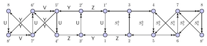
Figure 1: The quiver for $Y^{8,4}$ is shown to demonstrate the way we have numbered the nodes and faces of $Y^{p,q}$ quivers in general. The quivers are formed from impurity blocks with $Z$ or clean blocks with $V$ in them (see Herzog:2005 ). We draw the quiver in the most parity symmetric way with the impurity blocks in the middle. For even $p-q$, assign number 1 to the node in the middle with $Z$ leaving it, and the numbers increase along $Z$ and $U$ bifundamentals until node $p$ is arrived at. Note that for every numbered node in the quiver there is a mirror node that we denote with a prime. $S^{k}_{j}$ denote the coefficients of the superpotential couplings in (2); for every $S^{k}$ there is a mirror coefficient $S^{\prime k}=-S^{k}$ on the left that we have not shown in the figure. For odd $p-q$ there will be a single impurity block in the middle with $S^{k}_{0}=0$. Then number 1 is assigned to the node in the middle with $Z$ entering it.

As an example, we present the coefficients one obtains from (12) for the case $p=8,q=4$ shown in Figure 1:

$$\begin{split}&S^{a}_{1}=-S^{a}_{1^{\prime}}=-8,\ S^{a}_{2}=-S^{a}_{2^{\prime}}=16,\ S^{a}_{3}=-S^{a}_{3^{\prime}}=0,\ S^{a}_{4}=-S^{a}_{4^{\prime}}=24,\\ &S^{a}_{5}=-S^{a}_{5^{\prime}}=8,\ S^{a}_{6}=-S^{a}_{6^{\prime}}=16,\ S^{a}_{7}=-S^{a}_{7^{\prime}}=0,\ S^{a}_{8}=-S^{a}_{8^{\prime}}=8,\\ &S^{k}_{1}=-S^{k}_{1^{\prime}}=4,\ S^{k}_{2}=-S^{k}_{2^{\prime}}=12,\\ &S^{k}_{3}=-S^{k}_{3^{\prime}}=20,\ S^{k}_{4}=-S^{k}_{4^{\prime}}=4,\ S^{k}_{5}=-S^{k}_{5^{\prime}}=12,\ S^{k}_{6}=-S^{k}_{6^{\prime}}=-4.\end{split}$$

In particular, from the above coefficients the following expression for $\mathcal{B^{I}}_{Y^{8,4}}$ is obtained

$$\begin{split}\mathcal{B^{I}}_{Y^{8,4}}=&-8(\mbox{Tr }W_{1}^{2}-\mbox{Tr }W_{1^{\prime}}^{2})+16(\mbox{Tr }W_{2}^{2}-\mbox{Tr }W_{2^{\prime}}^{2})+24(\mbox{Tr }W_{4}^{2}-\mbox{Tr }W_{4^{\prime}}^{2})\\ &+8(\mbox{Tr }W_{5}^{2}-\mbox{Tr }W_{5^{\prime}}^{2})+16(\mbox{Tr }W_{6}^{2}-\mbox{Tr }W_{6^{\prime}}^{2})+8(\mbox{Tr }W_{8}^{2}-\mbox{Tr }W_{8^{\prime}}^{2}).\end{split}$$ (13)

Similarly, it is the expression for the $S^{a}$ coefficients in (12) that has led us to propose (8) for general $Y^{p,q}$. Our main reason for proposing (8) is that, as explained above, it yields the expected forms in the special cases with $p=1$. Further partial support comes from the analysis of the Konishi anomaly equation in appendix A. Also, with (8) at hand it seems natural to expect (LABEL:eq:marginalCombination), and the latter equation will be supported in subsection 3.3. The way one is led to (LABEL:eq:marginalCombination) from (8) is as follows. Take the $Y^{1,1}=S^{5}/\mathbb{Z}_{2}$ example. If we assume that the undeformed theory has equal couplings for the two gauge factors and its gravity dual has zero vev for the complex $B_{2}$ field, then turning on the vev would be dual to turning on the deformation operator (10). Therefore the vev in the deformed gravity theory would be proportional to the difference of the gauge couplings in the deformed field theory. That the proportionality constant in (LABEL:eq:marginalCombination) is correct will be argued in subsection 3.3. Note that the $S^{k}$ coefficients, if nonzero, would signal the required tuning of the superpotential couplings in the deformation, but do not enter (LABEL:eq:marginalCombination) themselves.

Rather than proving the relations in (12) we demonstrate their validity, and in fact only partially; the interested reader can complete the analysis along similar lines. Consider a case where $p-q$ is even, so that the quiver looks like Figure 1. Take two nodes numbered $2l+1$ and $2l+2\leq p-q$ according to the procedure explained under Figure 1. These are connected by a $Z$ chiral bifundamental that participates in two quartic superpotential terms that enter in the deformation with coefficient $S^{k}_{l+1}$. Equation (3) applied to the bifundamental superfield $Z$ reads

$$S^{a}_{2l+1}+S^{a}_{2l+2}=2S^{k}_{l+1}.$$

It is easy to check that this equation is satisfied by the coefficients in (12) since we have $S^{a}_{2l+1}=-p+2lq$, $S^{a}_{2l+2}=p+(2l+2)q$, and $S^{k}_{l+1}=(2l+1)q$. Similar computations can demonstrate the full validity of (12).

We take a moment to remind the reader that if one wanted to find only the $S^{a}$ coefficients, they would have an easier job since the $S^{a}$ coefficients can be obtained from the knowledge of the baryonic charges via ($S^{a}_{t(I)}-S^{a}_{h(I)}=Q_{J}(X_{I})$). But to find the $S^{k}$ coefficients as well, one should solve (3).

Important features of the solution

The first important feature of the solution in (12) that we would like to point out is that unless $q=0$ (corresponding to orbifolds of $T^{1,1}$) the coefficients $S^{k}$ are non-zero; this means that moving along this marginal direction requires not only changing a linear combination of the (inverse squared of the) gauge couplings, but also tuning the superpotential couplings in an appropriate way. This was pointed out in Benvenuti:2005a .

The coefficients with which the gauge couplings appear in this marginal combination are of most importance to us. The following relations that are satisfied by $S^{a}$ turn out to be useful in the next section:

$$\sum_{j=1}^{p-q}(-1)^{j+p-q}S^{a}_{j}=(p^{2}-q^{2}),$$ (14)

$$\sum_{j=p-q+1}^{p}(-1)^{j+p-q}S^{a}_{j}=q^{2}.$$ (15)

The First sum is over (half of) the impurity nodes and the second sum over (half of) the clean nodes.

3.3 Adding fractional branes

In Klebanov:2002 it was demonstrated that the chiral anomaly of the cascading gauge theory dual to the KS geometry Klebanov:2000 can be understood from the bulk point of view as Higgs mechanism. The massless scalar in the Betti hyper multiplet is eaten by the graviphoton (which in the absence of fractional branes gauges the U(1)_R in the bulk) leading to the bulk vector acquiring mass and hence the loss of current conservation from the boundary point of view. It is of no surprise then, that our identification of the operator dual to the Betti hyper in $Y^{p,q}$ allows us to investigate the effects of adding fractional branes in these geometries.

One may a priory expect that, similar to what Klebanov and Strassler did with $T^{1,1}$, one can add fractional branes to $Y^{p,q}$ geometries and study such phenomena as chiral symmetry breaking and confinement in the related quivers from the gravity side. A perturbative attempt to construct one such complete supergravity solution for $Y^{p,q}$ was made in Burrington:2005zd , based on the asymptotic solution of Herzog:2005 , but their approach was obstructed by the absence of complex deformations of the singularity at the tip of the cone over $Y^{p,q}$. This was later interpreted as absence of a supersymmetric vacuum in such theories and evidence was proposed for a runaway behavior in the general case Berenstein:2005xa ; Franco:2005 ; Bertolini:2005 ; Brini:2006 . However, for the $q=0$ cases corresponding to $T^{1,1}/\mathbb{Z}_{p}$, confinement and chiral symmetry breaking are expected for the field theories, and the gravity dual (being a $Z_{p}$ orbifold of the KS solution) confirms the expectations Franco:2005fd .

In this paper we only use the large-$r$ behavior of the solution given in Herzog:2005 as a guide for relating the CFT couplings and the gravity modulus, similar to what was done in Klebanov:2002 (see also Bertolini:2001 ; Bertolini:2002 ). We are assuming that this essentially UV computation is valid despite the out-of-control IR regime of general cascading $Y^{p,q}$ quivers.

With the aid of our proposal in (LABEL:eq:marginalCombination), and following Klebanov:2002 (their equation (18)), we write

$$\sum_{j}S^{a}_{j}(\Theta_{j}-\Theta_{j^{\prime}})=\frac{1}{\pi\alpha^{\prime}}\int_{\Sigma_{2}}C_{2},\hskip 50.58878pt\sum_{i}\Theta_{i}\sim C,$$ (16)

with $C$ being the RR scalar. In the first equation we have used the fact that $S^{a}_{j}=-S^{a}_{j^{\prime}}$.

We are going to test the relations in (16) by a gravitational computation of their RHS and a field theoretical computation of their LHS. Note that the non-zero value of the $B_{2}$ field that we referred to in footnote 8 has no effect on (16).

3.3.1 The gravity side

The RHS of the second relation in (16) is easy to find: the RR scalar is zero, similarly to the case of $T^{1,1}$ discussed in Klebanov:2002 .

To find the RHS of the first relation in (16) we need $C_{2}$. Herzog, Ejaz and Klebanov Herzog:2005 give (in their equation (41)) the following expression for the RR 3-form in the background with $M$ fractional branes

$$F_{3}=\frac{M\alpha^{\prime}}{2}(p^{2}-q^{2})[\mathrm{d}\psi\wedge\omega_{2}+\mathrm{d}(\frac{-y\cos\theta}{2(1-y)}\ \mathrm{d}\phi\wedge\mathrm{d}\beta)],$$

with $\omega_{2}$ a two-form given by

$$\omega_{2}=\frac{\sin\theta}{2(1-y)}\mathrm{d}\theta\wedge\mathrm{d}\phi-\frac{1}{2(1-y)^{2}}\mathrm{d}y\wedge\mathrm{d}\beta-\frac{\cos\theta}{2(1-y)^{2}}\mathrm{d}y\wedge\mathrm{d}\phi.$$

The 3-form $F_{3}$ can be locally written as the differential of a 2-form whose $\psi$-dependent part is

$$C_{2}=\frac{M\alpha^{\prime}}{2}(p^{2}-q^{2})\psi\omega_{2},$$ (17)

quite similar to equation (16) in Klebanov:2002 . Also similar is the action of the Reeb vector, which is none other than $\psi\to\psi+2\epsilon$, assuming $\delta\beta=\delta\phi=\delta y=\delta\theta=0$ Gauntlett:2004b .

Equation (17) shows that to evaluate the RHS of the first relation in (16) the following integral is needed Herzog:2005

$$\int_{\Sigma_{2}}\omega_{2}=\frac{4\pi p^{2}}{3(p^{2}-q^{2})}(p+\sqrt{4p^{2}-3q^{2}}).$$

Combining (17), (16) and the above result for the integral, we obtain

$$\sum_{j}S^{a}_{j}(\Theta_{j}-\Theta_{j^{\prime}})=4M\epsilon p^{2}(p+\sqrt{4p^{2}-3q^{2}})/3.$$ (18)

3.3.2 The field theory side

Now let us do the field theoretical calculation. For future convenience we define

$$x=\frac{2p-\sqrt{4p^{2}-3q^{2}}}{3q^{2}}.$$ (19)

Note in particular that $x=\frac{1}{4p}$ when $q\rightarrow 0$, and $x=\frac{1}{3p}$ when $q=p$. The $R$-charges of various bifundamental fields in the quivers are now expressed as

$$r_{U}=2px,\quad r_{V}=1-qx,\quad r_{Y}=1-(2p-q)x,\quad r_{Z}=1-(2p+q)x.$$ (20)

The coefficients $\rho$ appearing in the following are to be multiplied by

$$\frac{M}{16\pi^{2}}(F^{a\ ij}\tilde{F}^{a}_{ij})_{\mbox{node}},$$

and then summed over all the gauge factors to yield the anomalous divergence of the chiral $R$-current. $\rho$ can also be easily related to $\Theta$ angles (as in Klebanov:2002 ) via

$$\Theta=2\rho M\epsilon.$$ (21)

A simple field theoretical computation of the chiral anomaly for general $Y^{p,q}$ (reproduced in appendix B) yields

$$\rho^{p,q}_{\text{\footnotesize{imp }}j}=(-1)^{j+p-q}\left(p+q^{2}x\right),$$ (22)

and

$$\rho^{p,q}_{\text{\footnotesize{cl }}j}=(-1)^{j+p-q}\left(p+q^{2}x-2p^{2}x\right).$$ (23)

Note that $(-1)^{j+p-q}$ is positive if the impurity (respectively clean) node has a bifundamental field $Z$ (respectively $V$) entering it, and negative otherwise.

Using (22) and (23), one can obtain from (21)

$$\Theta^{p,q}_{\text{\footnotesize{imp}}}=(-1)^{j+p-q}2M\epsilon\left(p+q^{2}x\right),$$ (24)

and

$$\Theta^{p,q}_{\text{\footnotesize{cl}}}=(-1)^{j+p-q}2M\epsilon\left(p+q^{2}x-2p^{2}x\right).$$ (25)

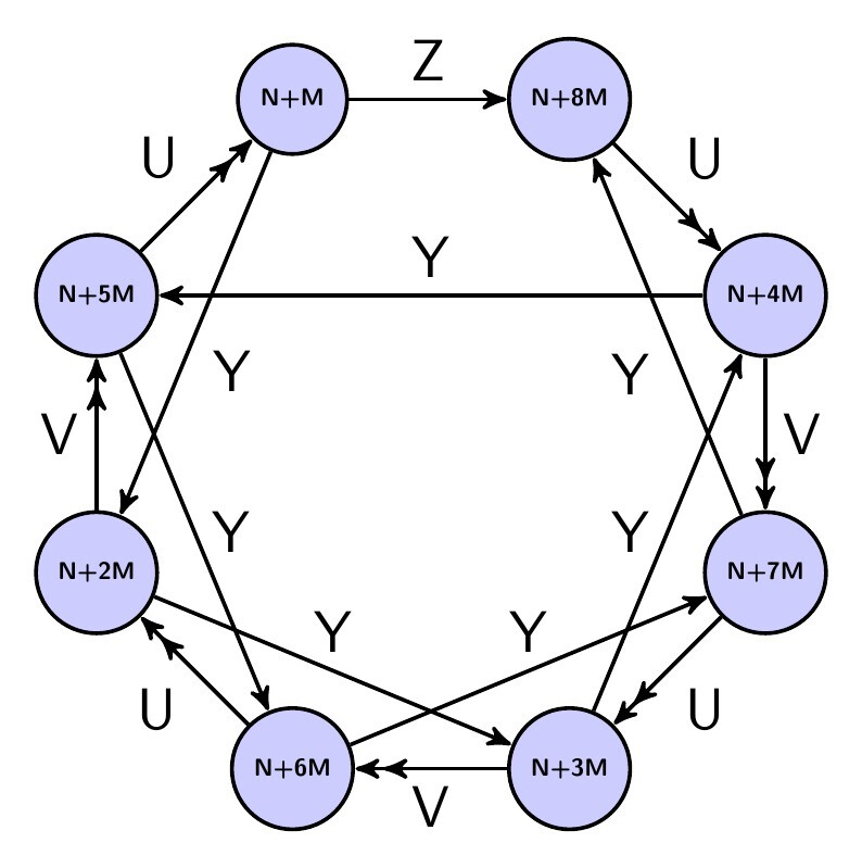
Figure 2: The cascading quiver obtained from $Y^{4,3}$.

As an example, for $Y^{4,3}$ (shown in Figure 2), we have $x=\sqrt{37}/27$, so

$$\begin{split}\partial_{i}J^{i}=&\frac{M}{16\pi^{2}}[-(p+q^{2}x)(F^{a\ ij}\tilde{F}^{a}_{ij})_{N+M}+(p+q^{2}x)(F^{a\ ij}\tilde{F}^{a}_{ij})_{N+8M}+\\ &(p+q^{2}x-2p^{2})(F^{a\ ij}\tilde{F}^{a}_{ij})_{N+2M}-(p+q^{2}x-2p^{2})(F^{a\ ij}\tilde{F}^{a}_{ij})_{N+7M}\\ &-(p+q^{2}x-2p^{2})(F^{a\ ij}\tilde{F}^{a}_{ij})_{N+3M}+(p+q^{2}x-2p^{2})(F^{a\ ij}\tilde{F}^{a}_{ij})_{N+6M}+\\ &(p+q^{2}x-2p^{2})(F^{a\ ij}\tilde{F}^{a}_{ij})_{N+4M}-(p+q^{2}x-2p^{2})(F^{a\ ij}\tilde{F}^{a}_{ij})_{N+5M}].\\ \end{split}$$

3.3.3 Consistency of the gravitational and field theoretical results

The second relation in (16) is obviously satisfied since $\Theta_{j}$ come in pairs with opposite sign $\Theta_{j^{\prime}}=-\Theta_{j}$ and therefore add up to zero, consistent with vanishing of $C$ in the dual backgrounds.

From (24) and (25) we can now check equation (18):

$$\begin{split}\sum_{j}S^{a}_{j}(\Theta_{j}-\Theta_{j^{\prime}})&=2(p^{2}-q^{2})|\Theta_{\mbox{\footnotesize{imp}}}|+2q^{2}|\Theta_{\mbox{\footnotesize{cl}}}|\\ &=4M\epsilon p^{2}(p-q^{2}x).\end{split}$$ (26)

To write the first equation we have employed the relations (14) and (15), with the extra fact that $\Theta_{j^{\prime}}=-\Theta_{j}$.

Note that if we had not found matching as in (26), we could have proposed that the missing relative factor must be inserted in the initial proposals (8) and (LABEL:eq:marginalCombination). Our success, however, supports the relations (8) and (LABEL:eq:marginalCombination) as they are.

4 Further examples with the general algorithm

In this section we want to explore the difficulties that arise when searching for exactly marginal operators dual to $B$ field moduli in more general toric geometries than $Y^{p,q}$. A particularly interesting class of more general toric SE₅ manifolds is $L^{a,b,c}$ Cvetic:2005 ; Franco:2006 ; Butti:2005bf .

Before examining specific examples, let us start by a few general remarks. One may hope to find exactly marginal directions of general $L^{a,b,c}$, similar to what we did for $Y^{p,q}$. When smooth, $L^{a,b,c}$ manifolds have the same topology as $Y^{p,q}$, hence they possess precisely one B-deformation. We did not succeed in finding a general expression (something similar to (12)) for this exactly marginal direction. This is because we did not manage to find an efficient general representation for the $L^{a,b,c}$ quivers. For $Y^{p,q}$ quivers such general representation was explained in Figure 1. Therefore we now turn to specific members of the $L^{a,b,c}$ family and look for possibly new features of their B-deformations.

Our first example in this section is $L^{1,5,2}$. The quiver theory was given explicitly in the appendix of Franco:2006 . We start by forming $B_{K}$ of this quiver. From the general formula $N_{f}=a+3b$ Franco:2006 , we quickly see that $B_{K}$ is a $16\times 16$ matrix. The null vectors of $B^{T}_{K}$ give the exactly marginal directions, as explained in section 2. We omit the details and only report the result. There are three such vectors. The three dimensional space spanned by these vectors certainly contains the directions corresponding to the sum of gauge couplings and the $\beta$-deformation. Therefore, two out of the three vectors can be safely substituted by $(1,1,...,1)^{T}$ and $(0,...,0,1,-1,...,1,-1)^{T}$, corresponding respectively to the sum of the gauge couplings and the $\beta$-deformation. A Gram-Schmidt procedure will then find the combination perpendicular to the previous two, which is dual to the $B$-field modulus. However, because the normalization of the null vectors is arbitrary, a proposal like (LABEL:eq:marginalCombination) can only be made up to an overall factor. The overall factor can then be determined by further inspection of the geometries deformed by adding fractional branes, as in subsection 3.3.

As the next example we consider $L^{1,2,1}$, also known as the Suspended Pinch Point (SPP). The geometry contains a codimension four singularity and is not smooth Franco:2006 . Hence, it is not surprising to see new features arise in this case. The details of this example are given in the appendix C. In the following we highlight the procedure.

The related Konishi matrix is $7\times 7$. After forming $B_{K}$ and finding the null vectors of its transpose, we find four exactly marginal directions. Two of them are again the sum of the gauge couplings and the $\beta$-deformation. The other two can be obtained by a Gram-Schmidt procedure, and are dual to the $B$-field moduli. The additional one, compared to $L^{1,5,2}$, arises because $L^{1,2,1}$ is singular and has a fixed circle; the fixed circle gives rise to a twisted sector that presumably contains (rather similar to the case of $S^{5}/\mathbb{Z}_{2}$ mentioned in subsection 3.1) a Betti hyper multiplet with a modulus inside it. The remaining piece of work would be to put the two B-deformations in one-to-one correspondence with the two-cycles in the dual geometry. This is achieved by comparing $S^{a}_{t(I)}-S^{a}_{h(I)}$ of the B-deformations, with the baryonic charge assignments $Q_{J}(X_{I})$ of the smooth two-cycle given in Table 1 of Franco:2006 . The exactly marginal direction consistent with the baryonic charge assignment of the smooth two-cycle corresponds to that two-cycle, and the orthogonal exactly marginal direction corresponds to the (blown-up) fixed circle.

Similarly, for cases with more than two B-deformations, help from the geometry side is needed to determine the appropriate baryonic charge assignments. Then these charge assignments can serve to disentangle the B-deformations into an orthogonal set whose members are in a one-to-one correspondence with the non-trivial two-cycles in the dual geometry.

5 Summary and discussion

In this paper we simultaneously completed the identification of the exactly marginal directions of generic $Y^{p,q}$ theories, and the determination of the protected operators dual to their shortened supergravity multiplets. The exactly marginal operator that we have found is dual to the $B$-field modulus of the gravity side. This modulus is incarnated at the linear level as a scalar component of a Betti hyper multiplet in the supergravity KK spectrum. The superfield version of the exactly marginal operator is thus dual to the Betti hyper multiplet.

We found the exactly marginal direction from the NSVZ equations, in the language developed in Imamura:2007 . In this approach, which applies to gauge theories described by brane tiling, finding exactly marginal operators boils down to solving a system of difference equations with coefficients $\pm 1$ (or $2$ if there are adjoint chiral fields in the gauge theory). We showed that the solutions to these equations can be thought of as left null vectors of a neatly derivable matrix, that we referred to as the Konishi matrix of the quiver, and denoted by $B_{K}$. The left nullity of the Konishi matrix (which equals its nullity, since the matrix is $N_{f}\times N_{f}$) is $2+b_{3}($SE${}_{5})$: one null direction corresponds to the sum of the gauge couplings, another corresponds to the $\beta$-deformation, and the remaining $b_{3}($SE${}_{5})$ correspond to the exactly marginal deformations dual to the $B$-field moduli. We called the last set B-deformations. Unlike the $\beta$-deformation, B-deformations do not break any global symmetry. We saw in section 3 that B-deformations generically involve tuning the superpotential couplings. It is not difficult to show that they always involve tuning of at least some of the gauge couplings; this is proved in appendix A.

We further pointed out that any set of baryonic charge assignments to matter fields gives a right null vector of $B_{K}$, but not every right null vector of $B_{K}$ yields a consistent baryonic charge assignment. This is because $B_{K}$ encodes only local data on the tiling. The two non-trivial cycles of the torus on which the tiling is defined impose two additional consistency relations on the baryonic charge assignments. Thus, only a codimension two subspace of the null space of $B_{K}$ corresponds to consistent baryonic charge assignments. This conclusion is obvious in retrospect as a codimension two subspace of the null space of $B_{K}$ would be $b_{3}($SE${}_{5})$ dimensional, and this is the number of global baryonic U(1) symmetries of the field theory.

In appendix A it is shown that the Konishi matrix can alternatively be thought to arise from Konishi anomaly equations. This point of view is advantageous, as compared to that of the NSVZ equations, in that it helps to frame the analysis in the context of the chiral ring of the field theory. Also, this viewpoint enables us to recognize the usefulness of the Konishi matrix beyond toric gauge theories.

There are various problems that follow naturally from our investigation. One important issue which deserves further study is that relation (LABEL:eq:marginalCombination) is only correct up to an additive constant that we have not been able to compute; see our comment in footnote 8. It would be nice to have a systematic approach to compute this constant for arbitrary toric theories. Another problem is that we have not found a solid argument to support our conjecture, presented in (4), for the form of the exactly marginal primary operators that deform gauge and superpotential couplings. We have provided partial support for our conjecture below equation (13), and also in appendix A. However, it would be highly desirable to have a sharp argument establishing (or ruling out) the form (4) for these operators.

In this paper we focused only on exactly marginal deformations that can be obtained by changing couplings already present in the original theories. As mentioned at the end of section 2 and in subsection 3.1, more exactly marginal directions may exist, which following Imamura:2007 we referred to as “accidentally marginal”. These would arise from mesonic exactly marginal chiral primary operators absent in the superpotential. For example, the conifold theory, the $\mathcal{N}=4$ theory, and $Y^{2,1}$ quiver theory, with respective global non-R symmetries SU(2)$\times$SU(2), SU(3), and SU(2)$\times$U(1), have respectively two, one, and zero accidentally marginal directions. It would be interesting to study theories admitting such accidentally marginal deformations to see if the following rule of thumb can be made more precise: a larger global symmetry group yields a larger conformal manifold. A precise version of the previous statement was conjectured by Kol Kol:2002 , in a form that neglects B-deformations and the exactly marginal direction dual to the axion-dilaton. For the remaining directions (including the $\beta$-deformation) Kol:2002 realizes the importance of the symmetric representation of the global flavor group in determining the dimensionality of the conformal manifold. However, as it stands, the conjecture of Kol:2002 is not correct for the known toric quivers, and it is not clear how to amend it. Therefore, it seems that more work is required to make the above rule of thumb precise. To that end, the analysis of Green:2010 would arguably play a key role, but needs to be supplemented with a method to first obtain the number of marginal chiral primary operators of a quiver. Note that since according to Green:2010 the global flavor group can make some of the marginal chiral primaries irrelevant (in a manner rather analogous to the Higgs mechanism), our rule of thumb needs that the number of marginal chiral primaries grow fast enough with the size of the flavor group to (over)compensate the loss of exactly marginal primaries; although this is the case in all the examples we are aware of, we have no proof why this should be true in general. We hope to report more progress on this in the future.

Appendix A Proofs for the properties of the Konishi matrix

In section 2 it was stated that every baryonic charge assignment satisfying (5) gives an $N_{f}$ tuple $(Q_{J}(X_{1}),...,Q_{J}(X_{N_{f}}))^{T}$ that is a null vector of $B_{K}$. This is seen to be true by noting that any of the first $N_{g}$ rows of

$$B_{K}\times(Q_{J}(X_{1}),...,Q_{J}(X_{N_{f}}))^{T}=0$$ (27)

imposes the first condition in (5) for the corresponding node in the quiver, while any of the last $N_{W}$ rows of (27) imposes the second condition in (5) for the corresponding superpotential loop in the quiver.

The second property of $B_{K}$ cited in the main text is that every set of coefficients $S^{a}$, $S^{k}$ that gives an exactly marginal direction of the form (6), yields an $N_{f}$ tuple

$$(S^{a}_{1},...,S^{a}_{N_{g}},S^{k}_{1},...,S^{k}_{N_{W}})$$

that is a left null vector of $B_{K}$. This is true because every column of

$$(S^{a}_{1},...,S^{a}_{N_{g}},S^{k}_{1},...,S^{k}_{N_{W}})\times B_{K}=0$$ (28)

is equivalent to the relation (3) for the corresponding chiral field (recall that columns of $B_{K}$ are labeled by the chiral fields in the quiver).

We now show the important fact that the left null vectors of $B_{K}$ are in one-to-one correspondence with the chiral primaries that one can form with Tr$W_{j}^{2}$ and $W_{m}$. To see this, consider a chiral bifundamental field $\Phi_{I}$ (the modifications required for adjoint chiral fields are straightforward), and define $J_{I}=\mathrm{Tr}\Phi_{I}e^{V_{h(I)}}\bar{\Phi}_{I}e^{-V_{t(I)}}$. Then from the Konishi anomaly equation we have

$$\frac{32\pi^{2}}{N}\bar{D}^{2}J_{I}=\sum_{j\in I}(TrW_{j}^{2})+\sum_{m\in I}(\frac{32\pi^{2}}{N}W_{m}).$$ (29)

Notice that the coefficients on the RHS are the entries of the Konishi matrix in the $I$th column, except for the reversed sign of the $W_{m}$ coefficients. A linear combination of Tr$W_{j}^{2}$ and $W_{m}$ that is a chiral primary should be perpendicular to the RHS of (29) for every $I$. There are $N_{f}$ relations like (29)—one for each $I$. There are also $N_{f}$ operators of the form Tr$W_{j}^{2}$ or $W_{m}$—$N_{g}$ of the former, and $N_{W}$ of the latter. Thus if the RHS of (29) for every $I$ gave a different expression, the orthogonalization procedure would leave no linear combination of Tr$W_{j}^{2}$ and $W_{m}$ as a chiral primary. But every time a linear combination of $\bar{D}^{2}J_{I}$ vanishes, there is one fewer constraint on the chiral primary combinations of Tr$W_{j}^{2}$ and $W_{m}$, and therefore one more of such chiral primaries. That these marginal chiral primary operators are indeed exactly marginal can then be deduced from either NSVZ, AdS/CFT, or a symmetry analysis as in Green:2010 . Note that if we knew how to perform the orthogonalization procedure mentioned above, it would give us the correction terms proportional to $W_{m}$ in the chiral primary combinations, and that would yield the required tuning of the superpotential couplings on the conformal manifold. But at least for a B-deformation with $S^{k}_{m}=0$ (as in that of $Y^{p,0}$), it already seems natural to expect that operators of the form (4) are perpendicular to all $\bar{D}^{2}J_{I}$ in (29).

Despite our inability to carry out the orthogonalization procedure referred to earlier, we conjecture that the primary operators perpendicular to (29) are of the form

$$\sum_{j}S^{a}_{j}(TrW_{j}^{2})-\sum_{m}S^{k}_{m}(\frac{32\pi^{2}}{N}W_{m}).$$ (30)

This conjecture is motivated by the following argument. At weak coupling, $g^{\prime}$ (defined below equation (2)) can be identified with the holomorphic coupling $g_{h}$. Then it is not difficult to see that small variations in one of the combinations (2), while keeping constant the rest, are indeed generated by adding operators of the form (30) to the superpotential. The apparent mismatch between the factor of 8 in (2) and the factor of 32 in (30) is explained by noting that $\mathcal{L}_{h}=\frac{1}{4}\int\mathrm{d}^{2}\theta W^{2}/g_{h}^{2}$. Note also that (30) gives the expected operator for the $\beta$-deformation, which has $S^{a}_{j}=0$ and $S^{k}_{m}=\pm 1$. This provides the further partial support for (4) that we promised in the main text.

Now, since $B_{K}$ is a square matrix, its left and right nullities are equal. This, however, does not mean that there are as many exactly marginal directions in the quiver as there are consistent baryonic charge assignments. The reason is that not every right null vector of $B_{K}$ gives a consistent baryonic charge assignment. This is because equation (27) imposes the second condition in (5) only on the superpotential loops in the quiver. As we show below, to find consistent baryonic charge assignments one should supplement (27) with two more relations, and hence only a codimension two subspace of the (right) null space of $B_{K}$ corresponds to consistent baryonic charge assignments.

One way to understand why the number two comes in, is to realize that ensuring the second condition in (5) on all loops in the quiver requires supplementing (27) by two relations arising from the two non-trivial cycles in the torus of brane tiling. To see this, note that any of the last $N_{W}$ rows of (27) imposes the second condition in (5) for the corresponding superpotential node in the tiling. Since brane tilings define bipartite graphs, each edge (i.e. chiral field) can be assigned a direction (e.g. from black nodes to white nodes) Franco:2006bd . With such directions assigned to the edges in brane tiling, one can interpret the second condition in (5) as Kirchhoff’s current law for arbitrary Gauss surfaces (that correspond to arbitrary loops in the quiver diagram) in ‘the brane tiling circuit’. We are thus interpreting the baryonic charge of a chiral field as the current its corresponding edge carries on brane tiling. Now, equation (27) ensures Kirchhoff’s current law on every node in the tiling, because nodes correspond to superpotential loops in the quiver. It is clear that this guarantees Kirchhoff’s current law for all shrinkable Gauss surfaces on the tiling. But to ensure the full consistency of the corresponding baryonic charge assignment, one has to add the two Kirchhoff current laws arising from the two non-trivial cycles in the torus on which the tiling is defined. These are the two relation that supplement (27) to give fully consistent baryonic charge assignments.

Instead of the argument of the previous paragraph, one could again use (29) to verify that for every null vector of $B_{K}$ there is one conserved current in the form of a linear combination of $J_{I}$, but two of the conserved currents are those of the global U(1)$\times$U(1) flavor symmetry of the CFT (equation (7) gives an example). Therefore a two dimensional subspace of the null space of $B_{K}$ corresponds to flavor U(1) charge assignments, and the rest of it to the baryonic charge assignments. The relation between the flavor U(1) symmetries and the non-trivial cycles of the tiling (which played a key role in the argument of the previous paragraph) is well-known (see for example Kennaway:2007 ). Also, from this argument it becomes clear in what sense the global non-$R$ U(1) symmetries are responsible for the $2+b_{3}($SE${}_{5})$ exactly marginal directions of toric quivers.

Finally, we show that B-deformations always involve tuning gauge couplings. In other words, there are no B-deformations with all their $S^{a}$ coefficients equal to zero. Let us assume there is one such deformation. Then starting with a node $P$ on brane tiling and considering the relation (3) for an edge $I$ connected to it, we see that the $S^{k}$ coefficient of the node $Q$ at the other end of $I$ should be negative of the $S^{k}$ coefficient of $P$. Then considering (3) for another edge $I^{\prime}$ connected to $Q$ and so on, we see that the $S^{k}$ coefficients on the tiling only alternate signs. This means we end up with the $\beta$-deformation (up to an insignificant normalization which is the value of $S^{k}$ chosen for the initial node $P$). Hence this is not a B-deformation.

To summarize, the Konishi matrix encodes local data on brane tiling. This local data is sufficient (and necessary) for determining the exactly marginal directions that we are concerned about (recall that in the present paper we are not concerned about the accidentally marginal directions, referred to at the end of section 2); these exactly marginal directions can be obtained from left null vectors of $B_{K}$. However, to determine the consistent baryonic charge assignments, the local data in $B_{K}$ (although necessary) must be supplemented by the global data encoded in the two nontrivial cycles of the torus of brane tiling; thus baryonic charge assignments form a codimension two subspace of the right null space of $B_{K}$.

Appendix B Field theoretical computation of $\Theta^{p,q}$ for the cascading $Y^{p,q}$ quivers

In this appendix, we prove the field theoretical relation (22). Equation (23) is derived similarly.

Figure 3: A typical impurity node in $Y^{p,q}$ quivers is shown as an empty node, with all its neighbors attached to it via chiral bifundamentals.

Take an impurity node $P$ that has a gauge factor of rank $N+kM$ with some $k$; this could be the empty node in Figure 3. Assume that the node has a bifundamental field singlet $Z$ ‘exiting’ it. This bifundamental would enter a node with rank $N+kM+pM+qM$, as dictated by the baryonic charge of $Z$ Benvenuti:2005b . There is also a bifundamental doublet $U$ entering $P$, which emanates from a node with rank $N+kM+pM$ as dictated by the baryonic charge of $U$. Finally, a bifundamental singlet $Y$ leaves $P$ to a destination node with rank $N+kM+pM-qM$ as dictated by the baryonic charge of $Y$. The chiral anomaly ($\mathrm{Tr}R$) of the fermions charged under $P$ is then given by

$$\begin{split}&\frac{1}{2}\times(N+kM+pM+qM)(r_{Z}-1)+2\times\frac{1}{2}\times(N+kM+pM)(r_{U}-1)\\ &+\frac{1}{2}\times(N+kM+pM-qM)(r_{Y}-1)+N+kM\\ &\ =-(p+q^{2}x)M,\end{split}$$

where we have used (20). In the above equation, the factors $\frac{1}{2}$ for the first three terms on the LHS are the Dynkin index of the fundamental representation, the extra coefficient $2$ for the second term is because $U$ is a doublet, and the fourth term is the gaugino contribution. A similar computation for a node which has a bifundamental field singlet $Z$ entering it yields the opposite sign, hence proving (22). The factors $(-1)^{j+p-q}$ appear because of the way we have numbered the nodes (see the caption of Figure 1).

Appendix C Exactly marginal directions for SPP

In this appendix we form the Konishi matrix of SPP quiver and obtain from it the exactly marginal directions in the space of couplings.

The quiver is shown in Figure 4. It contains seven chiral fields

$$V^{1}_{11},Y_{12},U^{1}_{13},U^{1}_{21},U^{2}_{23},Y_{31},Z_{32}.$$

The superpotential terms are Franco:2006

$$\begin{split}&W_{1}=U^{1}_{21}Y_{12}U^{2}_{23}Z_{32},\quad W_{2}=-Z_{32}U^{2}_{23}Y_{31}U^{1}_{13},\\ &W_{3}=U^{1}_{13}Y_{31}V^{1}_{11},\quad W_{4}=-Y_{12}U^{1}_{21}V^{1}_{11}.\end{split}$$

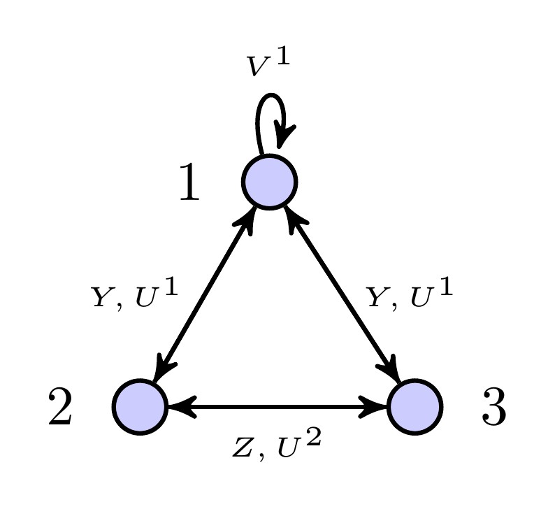
Figure 4: The quiver diagram for SPP. The chiral fields are named following Franco:2006 .

The Konishi matrix then follows to be

$$B_{K}=\begin{pmatrix}2&1&1&1&0&1&0\\ 0&1&0&1&1&0&1\\ 0&0&1&0&1&1&1\\ 0&-1&0&-1&-1&0&-1\\ 0&0&-1&0&-1&-1&-1\\ -1&0&-1&0&0&-1&0\\ -1&-1&0&-1&0&0&0\end{pmatrix}.$$ (31)

The four left null vectors are

$$(S^{a}_{1},S^{a}_{2},S^{a}_{3},S^{k}_{1},S^{k}_{2},S^{k}_{3},S^{k}_{4})= (1,1,1,1,1,1,1),$$

$$(0,0,0,1,-1,1,-1),$$

$$(0,2,-2,1,-1,-1,1),$$

$$(4,-3,-3,-3,-3,4,4).$$

The first two clearly correspond to the sum of gauge couplings and the $\beta$-deformation. The last two are B-deformations. The third one is consistent with the baryonic charge assignments for the smooth two-cycle (given in Table 1 of Franco:2006 ) and is therefore dual to the vev of the complex $B$ field on the smooth two-cycle. The last one is dual to the modulus inside the Betti hyper multiplet in the twisted sector arising from the fixed circle of $L^{1,2,1}$.

References

- (1) I. Klebanov and E. Witten, Superconformal field theory on threebranes at a Calabi-Yau singularity, Nucl. Phys. B 536 (1998) 199 [hep-th/9807080].
- (2) B. S. Acharya, J. M. Figueroa-O Farrill, C. M. Hull and B. Spence, Branes at conical singularities and holography, Adv. Theor. Math. Phys. 2 (1999) 1249 [hep-th/9808014].
- (3) D. R. Morrison and M. R. Plesser, Non-Spherical Horizons, I, Adv. Theor. Math. Phys. 3 (1999) 1 [hep-th/9810201].
- (4) J. P. Gauntlett, D. Martelli, J. Sparks and D. Waldram, Supersymmetric AdS5 solutions of M-theory, Class. Quant. Grav. 21 (2004) 4335 [hep-th/0402153].
- (5) J. P. Gauntlett, D. Martelli, J. Sparks and D. Waldram, Sasaki-Einstein metrics on , Adv. Theor. Math. Phys. 8 (2004) 711 [hep-th/0403002].
- (6) D. Martelli and J. Sparks, Toric Geometry, Sasaki-Einstein Manifolds and a New Infinite Class of AdS/CFT Duals, Commun. Math. Phys. 262 (2006) 51 [arXiv:0411238 [hep-th]].
- (7) M. Bertolini, F. Bigazzi and A. L. Cotrone, New checks and subtleties for AdS/CFT and a-maximization, JHEP 0412 (2004) 024 [hep-th/0411249].
- (8) S. Benvenuti, S. Franco, A. Hanany, D. Martelli and J. Sparks, An Infinite Family of Superconformal Quiver Gauge Theories with Sasaki-Einstein Duals, JHEP 0506 (2005) 64 [arXiv:hep-th/0411264].
- (9) S. Benvenuti and M. Kruczenski, Semiclassical strings in Sasaki-Einstein manifolds and long operators in N=1 gauge theories, JHEP 0610 (2006) 051 [arXiv:0505046 [hep-th]].
- (10) F. Canoura, J. D. Edelstein, L. A. Pando Zayas, A. V. Ramallo and D. Vaman, Supersymmetric branes on AdS and their field theory duals, JHEP 0603 (2006) 101 [hep-th/0512087].
- (11) C. P. Herzog, Q. J. Ejaz and I. R. Klebanov, Cascading RG flows from new Sasaki-Einstein manifolds, JHEP 0502 (2005) 009 [hep-th/0412193].
- (12) S. Benvenuti and A. Hanany, Conformal manifolds for the conifold and other toric field theories, JHEP 0508 (2005) 024 [hep-th/0502043].
- (13) O. Lunin and J. M. Maldacena, Deforming field theories with U(1)U(1) global symmetry and their gravity duals, JHEP 0505 (2005) 033 [hep-th/0502086].
- (14) A. A. Ardehali, J. T. Liu and P. Szepietowski, The shortened KK spectrum of IIB supergravity on , JHEP 1402 (2014) 064 [arXiv:1311.4550 [hep-th]].
- (15) D. Berenstein, C. P. Herzog, P. Ouyang and S. Pinansky, Supersymmetry Breaking from a Calabi-Yau Singularity, JHEP 0509 (2005) 084 [hep-th/0505029].
- (16) H. Kihara, M. Sakaguchi and Y. Yasui, Scalar Laplacian on Sasaki-Einstein Manifolds , Phys. Lett. B 621 (2005) 288 [hep-th/0505259].
- (17) R. Eager, J. Schmude and Y. Tachikawa, Superconformal Indices, Sasaki-Einstein Manifolds, and Cyclic Homologies, arXiv:1207.0573 [hep-th].
- (18) D. Martelli and J. Sparks, Symmetry-breaking vacua and baryon condensates in AdS/CFT, Phys. Rev. D 79 (2009) 065009 [hep-th/0804.3999].
- (19) A. A. Ardehali and P. Szepietowski, work in progress.
- (20) Y. Imamura, H. Isono, K. Kimura and M. Yamazaki, Exactly marginal deformations of quiver gauge theories as seen from brane tilings, Prog. Theor. Phys. 117(5) (2007) 923 [hep-th/0702049].
- (21) S. Franco, A. Hanany, D. Vegh, B. Wecht, and K. D. Kennaway, Brane dimers and quiver gauge theories, JHEP 0601 (2006) 096 [hep-th/0504110].
- (22) K. D. Kennaway, Brane tilings, International Journal of Modern Physics A 22, no. 18 (2007) 2977 [arXiv:0706.1660 [hep-th]].
- (23) I. R. Klebanov, P. Ouyang and E. Witten, A gravity dual of the chiral anomaly, [hep-th/0202056] (2002).
- (24) S. Franco, A. Hanany, D. Martelli, J. Sparks, D. Vegh and B. Wecht, Gauge theories from toric geometry and brane tilings, JHEP 0601 (2006) 128 [hep-th/0505211].
- (25) J. Terning, Modern supersymmetry: Dynamics and duality, Oxford University Press (2006).
- (26) C. P. Herzog and J. Walcher, Dibaryons from Exceptional Collections, JHEP 0309 (2003) 060 [hep-th/0306298v3].
- (27) D. Green, Z. Komargodski, N. Seiberg, Y. Tachikawa and B. Wecht, Exactly marginal deformations and global symmetries, JHEP 1006 (2010) 1 [arXiv:1005.3546 [hep-th]].
- (28) D. Baumann et al., D3-brane Potentials from Fluxes in AdS/CFT, JHEP 1006 (2010) 1 [arXiv:1001.5028 [hep-th]].
- (29) A. A. Ardehali, J. T. Liu and P. Szepietowski, corrections to the holographic Weyl anomaly, JHEP 1401 (2014) 002 [arXiv:1310.2611 [hep-th]].
- (30) C. P. Herzog, I. Klebanov, and P. Ouyang, Remarks on the Warped Deformed Conifold, [hep-th/0108101].
- (31) A.E. Lawrence, N. Nekrasov and C. Vafa, On conformal field theories in four dimensions, Nucl. Phys. B 533 (1998) 199 [hep-th/9803015].
- (32) I. R. Klebanov and M. J. Strassler, Supergravity and a confining gauge theory: Duality cascades and chiSB-resolution of naked singularitie, JHEP 0008 (2000) 052 [hep-th/0007191].
- (33) B. A. Burrington, J. T. Liu, M. Mahato and L. A. Pando Zayas, Towards supergravity duals of chiral symmetry breaking in Sasaki-Einstein cascading quiver theories, JHEP 0507 (2005) 019 [hep-th/0504155].
- (34) S. Franco, A. Hanany, F. Saad and A M. Uranga, Fractional Branes and Dynamical Supersymmetry Breaking, JHEP 0601 (2006) 011 [hep-th/0505040].
- (35) M. Bertolini, F. Bigazzi and A. L. Cotrone, Supersymmetry breaking at the end of a cascade of Seiberg dualities, Phys. Rev. D 72 (2005) 061902 [hep-th/0505055].
- (36) A. Brini and D. Forcella, Comments on the non-conformal gauge theories dual to Ypq manifolds, JHEP 0606 (2006) 050 [hep-th/0603245].
- (37) S. Franco, A. Hanany and A. M. Uranga, Multi-Flux Warped Throats and Cascading Gauge Theories, JHEP 0509 (2005) 028 [hep-th/0502113].
- (38) M. Bertolini, P. Di Vecchia, M. Frau, A. Lerda and R. Marotta, N=2 gauge theories on systems of fractional D3/D7 branes, Nucl. Phys. B 621, (2002) 157 [hep-th/0107057].
- (39) M. Bertolini, P. Di Vecchia, M. Frau, A. Lerda and R. Marotta, More Anomalies from Fractional Branes, Phys. Lett. B 540 (2002) 104 [hep-th/0202195].
- (40) M. Cvetic, H. Lu, D. N. Page and C. N. Pope, New Einstein-Sasaki spaces in five and higher dimensions, Phys. Rev. Lett. 95 (2005) 071101 [hep-th/0504225].
- (41) A. Butti, D. Forcella and A. Zaffaroni, The dual superconformal theory for Lp, q, r manifolds, JHEP 0509 (2005) 018 [hep-th/0505220].
- (42) R. Eager, Brane Tilings and Non-Commutative Geometry, JHEP 1103 (2011) 026 [arXiv:1003.2862].
- (43) B. Kol, On conformal deformations, JHEP 0209 (2002) 046 [hep-th/0205141].
- (44) A. Ceresole, G. Dall’Agata, R. D’Auria and S. Ferrara, Spectrum of type IIB supergravity on AdS: Predictions on SCFT’s, Phys. Rev. D 61, (2000) 066001 [hep-th/9905226].
- (45) S. Benvenuti, A. Hanany and P. Kazakopoulos, The toric phases of the quivers, JHEP 0507 (2005) 021 [hep-th/0412279].