Exchange-based two-qubit gate for singlet-triplet qubits

Abstract

We analyse a simple exchange-based two-qubit gate for singlet-triplet qubits in gate-defined semiconductor quantum dots that can be implemented in a single exchange pulse. Excitations from the logical subspace are suppressed by a magnetic field gradient that causes spin-flip transitions to be non-energy-conserving. We show that the use of adiabatic pulses greatly reduces leakage processes compared to square pulses. We also characterise the effect of charge noise on the entanglement fidelity of the gate both analytically and in simulations; demonstrating high entanglement fidelities for physically realistic experimental parameters. Specifically we find that it is possible to achieve fidelities and gate times that are comparable to single- qubit states using realistic magnetic field gradients.

I Introduction

Semiconductor quantum dot systems have become an increasingly promising architecture for large-scale quantum computing Hanson et al. (2007); Kloeffel and Loss (2013), growing out of the seminal work of Loss and DiVincenzo Loss and DiVincenzo (1998). Any successful quantum computing architecture must, with high reliability and precision, be able to: encode information, perform universal logical operations, generate measurable results, and be scalable to allow for large computations DiVincenzo (2000). While various semiconductor materials have yielded promising results, including among others silicon Maune et al. (2012); Dehollain et al. (2014) and carbon Trauzettel et al. (2007); Bulaev et al. (2008) based structures; GaAs/AlGaAs heterostructures remain very popular due to the advanced techniques developed for this material by experimenters.

The original semiconductor proposal Loss and DiVincenzo (1998) recognised the two-level spin system of an electron localised in a gate-defined semiconductor quantum dot as a natural encoding of a qubit, which is now called the Loss-DiVincenzo qubit. Two-qubit control was to be provided by exchange coupling between the dots, which has been implemented by modifying the gate voltages that define the dots Petta et al. (2005); and is now a matter of routine practice. Single-qubit control is more challenging Koppens et al. (2006); Pioro-Ladrière et al. (2008); Obata et al. (2010); Nadj-Perge et al. (2010); Brunner et al. (2011), and is usually implemented using electrically driven spin resonance in the presence of magnetic field gradients that allow for individual addressing.

Various modifications to Loss-DiVincenzo qubits and their manipulation have been proposed, each trading off the relative simplicity of single electron spin qubit encoding for systems of greater redundancy, ease of implementation, and/or resilience to experimental noise. Among the most promising of these new proposals are the “singlet-triplet” qubits Levy (2002); Johnson et al. (2005); Hanson and Burkard (2007); Barthel et al. (2009); Bluhm et al. (2010); Barthel et al. (2012); Shulman et al. (2012); Stepanenko et al. (2012); Klinovaja et al. (2012); Dial et al. (2013), which will be the focus of this paper. Another promising candidate is the exchange-only qubit DiVincenzo et al. (2000); Laird et al. (2010); Gaudreau et al. (2012); Medford et al. (2013a, b); Doherty and Wardrop (2013), which encodes logical qubits in the spins of three electrons; allowing for full electronic control through the exchange interaction alone.

Singlet-triplet qubits encode logical information in a pair of electron spins. The logical subspace of these qubits is the two-dimensional subspace of a pair of electron spins that is not Zeeman-shifted in an applied magnetic field, making them resistant to global magnetic field fluctuations Levy (2002). Single qubit operations are performed using a (potentially static) magnetic field gradient and an exchange coupling between the dots. We describe these qubits in more detail in section III.1. Static magnetic field gradients have been demonstrated using dynamic nuclear polarisationFoletti et al. (2009); Gullans et al. (2010) and patterned nano-magnetsMcNeil et al. (2010); Takakura et al. (2010); with gradients as large as $100\,mT$. There have been several proposals for two-qubit operations, the realisation of any being sufficient for universality of quantum computation Lloyd (1995). The only two-qubit gate currently demonstrated in experiment uses capacitive coupling van Weperen et al. (2011); Shulman et al. (2012).

In this paper we present a proposal for an exchange-based two-qubit gate for neighbouring singlet-triplet qubits that can effect high fidelity operations in a single adiabatic pulse. The use of exchange coupling has the significant advantage that gates can be fast, with gate times comparable to single qubit operations. However, use of exchange coupling between singlet-triplet qubits typically causes spin-flip transitions that result in excursions from the qubit subspace, leading to so-called leakage errors. Such leakage errors are suppressed during our gate by a static magnetic field gradient that causes spin-flip transitions to violate energy conservation; and are further mitigated by the adiabatic pulsing of the inter-qubit exchange couplings. Our proposal does not depend on the details of the substrate in which the quantum dots are embedded, or the way in which the exchange coupling and magnetic field gradients are realised; allowing for novel effective fields and couplings to be used (e.g. Coello et al. (2010); Mehl et al. (2014)). In simulations incorporating physically realistic charge noise, we found that with static magnetic field gradients less than $100\,mT$, and gate times as short as $7\,ns$, our gate can perform with entanglement fidelities in excess of 99.9%. In this regime, our gate performs with similar fidelity to single qubit operations. Our study complements a similar proposal described by Klinovaja and collaborators Klinovaja et al. (2012), which considers pulse sequences as an alternative to adiabatic pulses for solving the problems of leakage, and focusses on spin orbit coupling and Overhauser noise instead of charge noise. In addition, Li and collaborators Li et al. (2012) describe several pulse sequences which can effect two-qubit gates; and Kestner Kestner et al. (2013), Wang Wang et al. (2014) and collaborators have developed pulse sequences which mitigate the effect of low-frequency Overhauser and charge noise. The notion of energetically suppressing leakage processes also appears in our two-qubit gate proposal Doherty and Wardrop (2013) for the resonant exchange qubit Taylor et al. (2013); Medford et al. (2013a), in which context the use of adiabatic pulses is also expected to lead to significant reduction in leakage.

Our two-qubit gate does not have some of the drawbacks of earlier proposals. The exchange-based two-qubit gate accompanying the original singlet-triplet qubit proposal Levy (2002) required a sequence of complicated exchange pulses between neighbouring singlet-triplet qubits. Apart from their complexity, these sequences also required very precise timing and negligible charge noise in order to minimise leakage. Capacitive two-qubit gate proposals Taylor et al. (2005); van Weperen et al. (2011); Shulman et al. (2012); Trifunovic et al. (2012) have the advantage of having actually been implemented, and being applicable for more widely spaced qubits; but it has proven difficult thus far to create large charge dipoles in singlet-triplet qubits, leading to gate times an order of magnitude slower than single qubit exchange gates Petta et al. (2005); van Weperen et al. (2011). There have been some promising proposals to strengthen capacitive interactions; such as floating gates Trifunovic et al. (2012). A more fundamental limitation is that charge noise in the control voltages couples into capacitive interactions unfavourably Shulman et al. (2012). In contrast, our proposal promises gates that can be implemented between nearest neighbours using relatively simple adiabatic pulses; with gate times comparable to single qubit operations, and a more favourable noise scaling that allows one to trade off gate speed for less sensitivity to charge noise.

This paper is organised as follows: in section II we describe a model for semiconductor quantum dot systems; in section III we describe the mechanics of our two-qubit operation; in section IV we introduce a model for charge noise in singlet-triplet systems; in section V we analytically investigate the performance of our gate subject to this charge noise model; in section VI we present the results of simulations of our two-qubit gate and compare with the results of the previous section; and in section VII we discuss the significance of these results.

II Physical Model

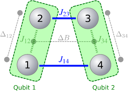
Figure 1: (colour online) Schematic diagram of a two singlet-triplet qubit configuration. The four quantum dots are indexed by $\{1,2,3,4\}$; and are slanted to indicate that a specific physical arrangement is unimportant. The intra-qubit exchange couplings required for single qubit operations are shown in dashed green ($J_{12}$ and $J_{34}$); and the inter-qubit couplings required for our two-qubit gate operation are shown in solid blue ($J_{14}$ and $J_{23}$). Important magnetic field gradients are depicted by thin broken grey lines joining solid discs; and labelled with the appropriate symbols: $\Delta B=\frac{1}{2}\left(B_{1}+B_{2}-B_{3}-B_{4}\right)$ and $\Delta_{ij}=B_{i}-B_{j}$.

In this section we introduce the model we use to describe exchange-coupled quantum dots; which we use in the following section to explain the mechanism of our proposed two qubit gate for singlet-triplet qubits.

We have chosen to model a system of $N$ electrons (each isolated in a gate-defined quantum dot) with the time dependent Heisenberg Hamiltonian:

$$H(t)=\mu\sum_{n=1}^{N}B_{n}(t)\sigma_{z}^{n}+\frac{1}{4}\sum_{\left<i,j\right>}J_{ij}(t)(\bm{\sigma}^{i}\cdot\bm{\sigma}^{j}-I),$$ (1)

where $\left<i,j\right>$ indicates that the sum should only include pairs of $i$ and $j$ if there exists non-negligible quantum tunnelling between quantum dots $i$ and $j$; and $\bm{\sigma}^{i}$ is the vector of Pauli operators $(\sigma_{x},\sigma_{y},\sigma_{z})$ acting on dot $i$. The first sum of terms describes Zeeman splitting of the spin states at each dot due to the local magnetic field $B_{n}(t)$; and the second describes the exchange couplings $J_{ij}(t)$ between the dots. We set $\hbar=1$ throughout this paper.

A large external magnetic field $B_{0}=\bm{B}_{0}^{z}=\frac{1}{4}\sum_{n}B_{n}$ creates a preferred orientation, which we arbitrarily label the $z$-axis. All of the magnetic fields $B_{n}$ are taken to be along this $z$-axis, as the effects of perpendicular fields will be suppressed provided $\bm{B}_{n}^{\perp}\ll\bm{B}_{n}^{z}$. We will find it useful to consider the magnetic fields in the following basis: the global background magnetic field $B_{0}=\frac{1}{4}\sum_{n}B_{n}$, the inter-qubit gradient $\Delta B=\frac{1}{2}\left(B_{1}+B_{2}-B_{3}-B_{4}\right)$, and the intra-qubit gradients $\Delta_{12}$ and $\Delta_{34}$ with $\Delta_{ij}=B_{i}-B_{j}$. Thus $B_{1}=B_{0}+\frac{1}{2}\Delta B+\frac{1}{2}\Delta_{12}$; and so on.

Computation using singlet-triplet qubits requires control of the exchange couplings $J_{ij}(t)$, which depend on the shape of the quantum dot potential wells that are in turn determined by electrode voltages that we parameterise by $\varepsilon_{ij}$; and so $J_{ij}(t)=J_{ij}(\varepsilon_{ij}(t))$. The precise dependence of $J_{ij}$ on $\varepsilon_{ij}$ is determined by the microscopic details of experimental apparatus. In order to make quantitative statements about our proposal, in section IV.2 we will consider a phenomenological fit to data from GaAs/AlGaAs singlet-triplet experiments.

This model can be regarded as an approximation of the more general Hubbard model with $N$ sites, local magnetic fields $\bm{B}_{n}(t)$ and tunnelling between sites $i$ and $j$ of $t_{ij}(t)$. The exchange coupling terms $J_{ij}(\bm{\sigma}\cdot\bm{\sigma}-II)$ are the second order perturbative effect of quantum tunnelling $t_{ij}$; with $J_{ij}=4t_{ij}^{2}/E_{C}$, where $E_{C}$ is the energy penalty associated with charging a quantum dot with two electrons. This approximation holds in the limit of weak tunnelling $t_{ij}\ll E_{\textrm{C}}$.

III Logical Operations

In this section we provide an intuition for how our gate works; before describing it in detail. The key physics that underpins the operation of our gate is the same as for single-qubit exchange gates; made more complicated by the possibility of low-energy excitations from the logical subspace. We suppress these by applying a gradient magnetic field to make spin-flip transitions non-energy-conserving; as also discussed in Klinovaja et al. Klinovaja et al. (2012). We first review single qubit gates.

III.1 Single Qubit Gates for Singlet-Triplet Qubits

Singlet-triplet qubits are encoded in the spins of two electrons, each isolated in a quantum dot (such as one of the qubits in figure 1); and are controlled using inter-dot magnetic field gradients and variable exchange coupling, in the presence of a strong global magnetic field. The Hamiltonian describing such a system is that given by equation (7) restricted to two dots ($N=2$).

The strong global magnetic field $B_{0}$ makes the spin basis a natural one for this system: $\left|\uparrow\uparrow\right>$, $\left|\uparrow\downarrow\right>$, $\left|\downarrow\uparrow\right>$, and $\left|\downarrow\downarrow\right>$, where the arrows indicate the $\hat{S}^{z}$ projection of the electrons’ spin. The global field $B_{0}$ Zeeman splits the $\sum\hat{S}^{z}\neq 0$ states from the $\sum\hat{S}^{z}=0$ states, which energetically suppresses the hyperfine interactions between the electron and semiconductor lattice nuclear spins that would otherwise cause excitations between them Petta et al. (2005). The singlet-triplet qubit is encoded in the two-dimensional $\sum\hat{S}^{z}=0$ subspace, which is spanned by the states $\{\left|\uparrow\downarrow\right>,\left|\downarrow\uparrow\right>\}$. The exchange term $\frac{1}{4}J_{12}(\bm{\sigma}^{1}\cdot\bm{\sigma}^{2}-I)$ has two eigenstates in the logical subspace: the singlet state $\left|S\right>=\left(\left|\uparrow\downarrow\right>-\left|\downarrow\uparrow\right>\right)/\mathchoice{{\hbox{$\displaystyle\sqrt{2\,}$}\lower 0.4pt\hbox{\vrule height=6.44444pt,depth=-5.15558pt}}}{{\hbox{$\textstyle\sqrt{2\,}$}\lower 0.4pt\hbox{\vrule height=6.44444pt,depth=-5.15558pt}}}{{\hbox{$\scriptstyle\sqrt{2\,}$}\lower 0.4pt\hbox{\vrule height=4.51111pt,depth=-3.6089pt}}}{{\hbox{$\scriptscriptstyle\sqrt{2\,}$}\lower 0.4pt\hbox{\vrule height=3.22221pt,depth=-2.57779pt}}}$ and the $\hat{S}_{z}=0$ triplet state $\left|T_{0}\right>=\left(\left|\uparrow\downarrow\right>+\left|\downarrow\uparrow\right>\right)/\mathchoice{{\hbox{$\displaystyle\sqrt{2\,}$}\lower 0.4pt\hbox{\vrule height=6.44444pt,depth=-5.15558pt}}}{{\hbox{$\textstyle\sqrt{2\,}$}\lower 0.4pt\hbox{\vrule height=6.44444pt,depth=-5.15558pt}}}{{\hbox{$\scriptstyle\sqrt{2\,}$}\lower 0.4pt\hbox{\vrule height=4.51111pt,depth=-3.6089pt}}}{{\hbox{$\scriptscriptstyle\sqrt{2\,}$}\lower 0.4pt\hbox{\vrule height=3.22221pt,depth=-2.57779pt}}}$; which are customarily chosen to be the computational basis states (hence the name “singlet-triplet” qubitPetta et al. (2005)).

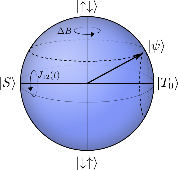
Figure 2: (colour online) Schematic showing the alignment of the single-qubit Bloch sphere. The magnetic field gradient $\Delta B$ rotates an arbitrary qubit state $\left|\psi\right>$ about the z-axis of the Bloch sphere, while the exchange interation $J_{12}$ rotates it about the x-axis.

Universal control of a qubit entails the ability to perform arbitrary rotations of Bloch vectors around the Bloch sphere, which requires two independent axes of rotation. For singlet-triplet qubits, these are provided by a static magnetic field gradient $\Delta B=B_{1}-B_{2}$ and a variable exchange coupling $J_{12}(t)$, as depicted in figure 2. In order to simplify discussion in this paper, we have chosen to orient the Bloch sphere such that the north and south poles are aligned with $\left|\uparrow\downarrow\right>$ and $\left|\downarrow\uparrow\right>$ respectively; and the x-axis with the singlet state $\left|S\right>=\left(\left|\uparrow\downarrow\right>-\left|\downarrow\uparrow\right>\right)/\mathchoice{{\hbox{$\displaystyle\sqrt{2\,}$}\lower 0.4pt\hbox{\vrule height=6.44444pt,depth=-5.15558pt}}}{{\hbox{$\textstyle\sqrt{2\,}$}\lower 0.4pt\hbox{\vrule height=6.44444pt,depth=-5.15558pt}}}{{\hbox{$\scriptstyle\sqrt{2\,}$}\lower 0.4pt\hbox{\vrule height=4.51111pt,depth=-3.6089pt}}}{{\hbox{$\scriptscriptstyle\sqrt{2\,}$}\lower 0.4pt\hbox{\vrule height=3.22221pt,depth=-2.57779pt}}}$ and the triplet state $\left|T_{0}\right>=\left(\left|\uparrow\downarrow\right>+\left|\downarrow\uparrow\right>\right)/\mathchoice{{\hbox{$\displaystyle\sqrt{2\,}$}\lower 0.4pt\hbox{\vrule height=6.44444pt,depth=-5.15558pt}}}{{\hbox{$\textstyle\sqrt{2\,}$}\lower 0.4pt\hbox{\vrule height=6.44444pt,depth=-5.15558pt}}}{{\hbox{$\scriptstyle\sqrt{2\,}$}\lower 0.4pt\hbox{\vrule height=4.51111pt,depth=-3.6089pt}}}{{\hbox{$\scriptscriptstyle\sqrt{2\,}$}\lower 0.4pt\hbox{\vrule height=3.22221pt,depth=-2.57779pt}}}$. This choice of Bloch axes is unconventional (e.g. Petta et al. (2005)); but allows us to describe the operation of our two-qubit gate in terms of diagonal Pauli z-operators in subsequent sections. In this basis, the magnetic field gradient causes coherent phase evolution of an arbitrary superposition $\left|\psi\right>=\alpha\left|\uparrow\downarrow\right>+\beta\left|\downarrow\uparrow\right>\mapsto\alpha\left|\uparrow\downarrow\right>+\beta\exp(i\mu\Delta Bt)\left|\downarrow\uparrow\right>$, which describes rotations about the z-axis of the Bloch sphere. It is sufficient for this field gradient to be static, since one can keep track of the precession. The exchange operator lowers the singlet state $\left|S\right>$ in energy by a controllable amount $J_{12}(t)$ compared to the triplet states $\{\left|\uparrow\uparrow\right>,\left|T_{0}\right>,\left|\downarrow\downarrow\right>\}$. This causes coherent phase evolution of an arbitrary superposition $\left|\psi\right>=\alpha\left|S\right>+\beta\left|T_{0}\right>\mapsto\alpha\left|S\right>+\beta\exp(-i\int_{0}^{t}J_{12}(t^{\prime})dt^{\prime})\left|T_{0}\right>$, which describes x-axis rotations around the Bloch sphere. When $\left|\psi\right>$ is an equal superposition of $\left|S\right>$ and $\left|T_{0}\right>$, these rotations are manifest as coherent oscillations between the $\left|\uparrow\downarrow\right>=\left|T_{0}\right>+\left|S\right>$ and $\left|\downarrow\uparrow\right>=\left|T_{0}\right>-\left|S\right>$ states. Together, these two operations can effect an arbitrary rotation in the Bloch sphere, and thus provide universal control.

To characterise single-qubit gate times for later comparison to two-qubit operations, we consider an application of a SWAP gate that has the effect of flipping the spins of the two electrons encoding the qubit state. This occurs when the qubit state $\left|\psi\right>$ is rotated about the x-axis of the Bloch sphere by $\pi$ radians, which is when $\int_{0}^{\tau}J_{12}(t)dt=\pi$ (c.f. Petta et al. (2005)), or when gate time $\tau=\pi/J_{12\,\mathrm{avg}}$.

III.2 Our Two Qubit Exchange Gate

The premise of our two-qubit gate proposal is to use exchange couplings $J_{14}$ and $J_{23}$ between two singlet-triplet qubits (as shown in figure 1) in order to perform a conditional phase gate (CPHASE) between the logical states of the two qubits.

There are four quantum dots in the combined two-qubit system, which are described by the Hamiltonian in equation 7 with $N=4$. Just as for the single qubit case, the strong background magnetic field makes the $2^{4}=16$ spin configurations a natural basis. The logical basis is the tensor product of the single qubit subspaces: $\{\left|\uparrow\downarrow,\uparrow\downarrow\right>,\left|\uparrow\downarrow,\downarrow\uparrow\right>,\left|\downarrow\uparrow,\uparrow\downarrow\right>,\left|\downarrow\uparrow,\downarrow\uparrow\right>\}$. Unlike the single qubit case, the logical subspace is not energetically isolated by the global magnetic field. There are two non-logical states (called “leakage” states) which also have $\sum\hat{S}^{z}=0$ : $\left|\uparrow\uparrow,\downarrow\downarrow\right>$ and $\left|\downarrow\downarrow,\uparrow\uparrow\right>$. This makes the system susceptible to zero-energy excitations from the logical subspace. To make matters worse, such leakage transitions are actually driven from the logical states $\left|\uparrow\downarrow,\uparrow\downarrow\right>$ and $\left|\downarrow\uparrow,\downarrow\uparrow\right>$ by the exchange couplings $J_{14}$ and $J_{23}$ that are necessary for our two-qubit gate.

The addition of a magnetic field gradient $\Delta B$ between the two qubits isolates the logical subspace from the leakage states by approximately $\mu\Delta B$. In the limit that exchange couplings $J_{14}$ and $J_{23}$ are much less than $\mu\Delta B$, transitions from the logical subspace to the unwanted $\sum\hat{S}^{z}=0$ states are energetically forbidden (and thus suppressed). We will later discuss the use of adiabatic activation of $J_{ij}$ to further suppress leakage. Note that the field gradient must be much smaller than the applied homogeneous field $\Delta B\ll B_{0}$, so that $B_{0}$ remains the dominant energy scale. Since leakage from the logical subspace can in principle be made negligible by choosing small enough $J_{ij}\ll\mu\Delta B\ll\mu B_{0}$, we postpone further discussion of leakage until section IV.1; and focus on perfectly adiabatic gate operation.

During the operation of our gate, we turn off intra-qubit exchange couplings $J_{12}$ and $J_{34}$; before activating $J_{14}$ and/or $J_{23}$. This effectively decouples the system into a new pairing of quantum dots which are described by exactly the same Hamiltonian as singlet-triplet qubits, but which are not confined to the singlet-triplet logical subspace. In particular, notice that if the two qubit system is initially in the logical state $\left|\uparrow\downarrow,\downarrow\uparrow\right>$, then the new pairings would lead to two-quantum-dot triplet states $\left|\uparrow\uparrow\right>$ and $\left|\downarrow\downarrow\right>$ that previously did not correspond to logical states.

As described in section III.1, activating exchange coupling between dots $i$ and $j$ lowers the singlet energy state by $J_{ij}$ compared to the relevant triplet states. Under $J_{14}$ and/or $J_{23}$, the logical states that have singlet character under the new pairings, $\left|\uparrow\downarrow,\uparrow\downarrow\right>$ and $\left|\downarrow\uparrow,\downarrow\uparrow\right>$, reduce in energy by approximately $\frac{1}{2}(J_{14}+J_{23})$ compared to the other two logical states, $\left|\uparrow\downarrow,\downarrow\uparrow\right>$ and $\left|\downarrow\uparrow,\uparrow\downarrow\right>$. This interaction looks like a logical $\sigma_{z}\sigma_{z}$ coupling between the two singlet-triplet qubits; which is well known to generate CPHASE gates modulo single qubit z-rotations (e.g. DiCarlo et al. (2009)) when the phase associated with $\sigma_{z}\sigma_{z}$ has accumulated to $\pi/2$. We will show more rigorously in the following that a CPHASE gate results after a time $\tau$ such that $\int_{0}^{\tau}\left[J_{14}(t)+J_{23}(t)\right]dt=\pi$; or $\tau=\pi/(J_{14}+J_{23})_{\textrm{avg}}$. Although it appears that our gate could be twice as fast as the singlet qubit SWAP gate (see section III.1), $[\sum J_{ij}]_{\textrm{avg}}$ is likely to be at least halved by the adiabatic pulses that are required for high fidelity operation (discussed in section IV). For a more experimentally achievable linear arrangement ($J_{23}=J$, $J_{14}=0$) using an adiabatic pulse, our gate would have operation times of roughly twice that of a single qubit SWAP gate with comparable fidelity.

We can formalise this argument by appealing to perturbation theory to further motivate the $\sigma_{z}\sigma_{z}$ coupling between the qubits. Since $J_{14}+J_{23}\ll B_{0}$, we can consider the exchange coupling terms ($V$) to be a perturbation to the Zeeman splitting terms $(H_{0}$) of the Hamiltonian in equation 7. The first order perturbed Hamiltonian will then be $H^{1}=H_{0}+PVP$, where $P$ is a projector onto the spin basis; and hence only the diagonal components of $V$ can affect the eigenstates of the Hamiltonian at first order. The exchange coupling operators are of the form $\bm{\sigma}\cdot\bm{\sigma}=\sigma_{x}\sigma_{x}+\sigma_{y}\sigma_{y}+\sigma_{z}\sigma_{z}$ (identity operators omitted), and so only the $\sigma_{z}\sigma_{z}$ terms will contribute; which when projected onto the logical subspace looks like a logical $\sigma_{z}\sigma_{z}$ interaction. The $\sigma_{x}\sigma_{x}$ and $\sigma_{y}\sigma_{y}$ components give rise to corrections at higher orders of perturbation theory; which nevertheless turn out to be correctable using single qubit phase gates.

Due to the simplicity of the model, we can in fact solve the system exactly for the eigenvalues and eigenstates by breaking the system down into a series of two-level systems; for example, for $J_{14}\neq 0$, the two level system of $\left|\uparrow\downarrow,\uparrow\downarrow\right>$ and $\left|\downarrow\downarrow,\uparrow\uparrow\right>$. The energies for all eigenstates are tabulated in the supplementary material. Since we are principally interested in the dynamics of the logical subspace, we restrict our attention to the states which adiabatically transform to the logical basis $\{\left|\uparrow\downarrow,\uparrow\downarrow\right>,\left|\uparrow\downarrow,\downarrow\uparrow\right>,\left|\downarrow\uparrow,\uparrow\downarrow\right>,\left|\downarrow\uparrow,\downarrow\uparrow\right>\}$ which we label $\{\left|1\right>\left|1\right>,\left|1\right>\left|0\right>,\left|0\right>\left|1\right>,\left|0\right>\left|0\right>\}$ respectively. We can then write a Hamiltonian, termed the “effective” Hamiltonian, that reproduces the instantaneous energy spectrum. Written in terms of effective Pauli operators $\tilde{\sigma}_{z}^{i}$ for qubit $i$, e.g. $\tilde{\sigma}_{z}^{1}=(\left|1\right>\left<1\right|-\left|0\right>\left<0\right|)\otimes I$, the resulting effective Hamiltonian is:

$$H_{\mathrm{eff}} = (\mu\Delta_{12}+\bar{B})\tilde{\sigma}_{z}^{1}+(\mu\Delta_{34}+\bar{B})\tilde{\sigma}_{z}^{2}$$ (2)

$$+\frac{1}{4}(J_{14}+J_{23})\left(\tilde{\sigma}_{z}^{1}\tilde{\sigma}_{z}^{2}-II\right),$$

with $\Delta_{ij}=B_{i}-B_{j}$ and $\bar{B}$ an effective global intra-qubit magnetic field that depends on $J_{ij}$ and the magnetic field gradients between each pair of dots. For the precise form of $\bar{B}$, refer to the supplementary material.

The effective Hamiltonian in equation (2) can be used to calculate the dynamical two-qubit phase accrued by adiabatic evolution of our gate; in which case our gate will perform a perfect CPHASE gate using a single exchange coupling pulse in a time $\tau=\pi/(J_{14}+J_{23})_{\textrm{avg}}$ modulo known correctable single qubit gates. One can either keep track of the single-qubit errors described by this Hamiltonian and later correct them after one or several gate operations, or correct them during the gate operation by various pulse sequences Klinovaja et al. (2012).

IV Sources of Error

Our proposed two-qubit gate will suffer from two main sources of error: leakage and environmental noise. Leakage from the logical subspace will occur due to excitations to the the non-logical $\sum\hat{S}^{z}=0$ states during the course of our gate, which we suppress in our proposal using a magnetic field gradient and adiabatic exchange pulses. While the basic mechanics of our gate are agnostic about the details of implementation, the nature of environmental noise depends very much on these details. In order to make quantitative predictions about the performance of our gate, we have chosen to mimic the noisy environment of GaAs/AlGaAs semiconductor systems. In these systems, we anticipate that charge fluctuations are likely to be the largest source of environmental noise; as was observed in single qubit singlet-triplet exchange experiments Dial et al. (2013). As a result, in this work we neglect the Overhauser field due to the bath of nuclear spins in the semiconductor lattice, which should be less significant than charge noise over the time-scale of a single gate, and which can in any case be suppressed, for example, by nuclear state preparation Reilly et al. (2008); Foletti et al. (2009). We also neglect the influence of spin-flip processes arising from spin orbit couplingKlinovaja et al. (2012), which have been shown to occur on millisecond time-scales Coish et al. (2007); Johnson et al. (2005) rather than the nanosecond time-scales in which we are interested.

IV.1 Leakage

We define leakage ($\mathcal{L}$) to be the probability that the state of the system, if measured, would not be in the logical subspace: $\mathcal{L}=1-\left<\psi\right|P\left|\psi\right>$, where $\psi$ is the state of the system, and $P$ is the projector onto the logical subspace. In the analysis of our two-qubit gate in section III.2, we restricted the domain of attention to the logical subspace; explicitly neglecting leakage. Without spin orbit coupling, leakage can only occur to other states in the $\sum\hat{S}^{z}=0$ subspace. Although leakage to the off-subspace states $\left\{\left|\uparrow\uparrow,\downarrow\downarrow\right>,\left|\downarrow\downarrow,\uparrow\uparrow\right>\right\}$ is suppressed by the energy gap $\mu\Delta B$ introduced by $\Delta B$, if the exchange coupling terms are too quickly varied, diabatic transitions will still occur and result in leakage probability oscillations with frequency $\sim\mu\Delta B/h$; as seen for the square (non-adiabatic) profile in figure 3b.

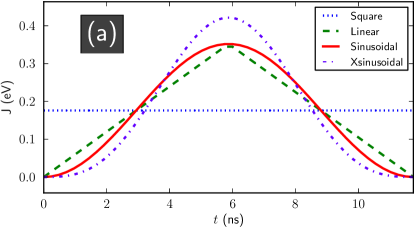
(a)

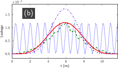
(b)

Figure 3: (colour online) a) The square, linear, sinusoidal and xsinusoidal adiabatic pulse profiles discussed in the text. Amplitudes are chosen to preserve gate operation time, and hence the average value of $J$. We have here chosen $J_{\mathrm{avg}}=0.18\,\mu eV$, which corresponds to a gate time of roughly $11.5\,ns$. b) Leakage from the logical subspace during the operation of the gate for each of the square, linear, sinusoidal and xsinusoidal pulses in (a). Note that the use of adiabatic profiles can significantly reduce leakage errors at the end of the gate operation.

Since the leakage is periodically returning to zero, it is in principle possible minimise leakage by using precise timing of the gate in a manner similar to Levy’s original proposalLevy (2002). However, this only works in the absence of other sources of noise, and is in practice very difficult in any case; and we suggest that the suppression of leakage using adiabatic pulses is substantially more robust.

An adiabatic pulse is one that turns on slowly and smoothly enough that the system remains in an instantaneous eigenstate. The rate at which a pulse can be turned on while remaining adiabatic depends on energy gap between the occupied eigenstates and their neighbours. In our case, two of the four logical states $\left\{\left|\uparrow\downarrow,\uparrow\downarrow\right>,\left|\downarrow\uparrow,\downarrow\uparrow\right>\right\}$ can leak to the states $\left\{\left|\uparrow\uparrow,\downarrow\downarrow\right>,\left|\downarrow\downarrow,\uparrow\uparrow\right>\right\}$, which are separated in energy by approximately $\mu\Delta B$.

While a pulse can never be perfectly adiabatic, even a very simple adiabatic pulse can greatly improve gate performance. In this paper, we have chosen to demonstrate the behaviour of adiabatic pulses using three representatives: linear, sinusoidal and “xsinusoidal”, which we compared to the non-adiabatic square pulse; as defined below:

$$J_{\textrm{sq}}(t) = J_{\textrm{avg}}=\frac{\pi}{\tau}$$

$$J_{\textrm{lin}}(t) = 2J_{\textrm{avg}}\left(1-\left|\frac{2t}{\tau}-1\right|\right)$$

$$J_{\textrm{sin}}(t) = J_{\textrm{avg}}\left(1-\cos\left(\frac{2\pi t}{\tau}\right)\right)$$

$$J_{\textrm{xsin}}(t) = J_{\textrm{avg}}\frac{6\pi^{2}}{(\pi^{2}+3)}\frac{t(\tau-t)}{\tau^{2}}\left(1-\cos\left(\frac{2\pi t}{\tau}\right)\right),$$

each of which is depicted in figure 3a. For ease of comparison, each profile has been normalised such that for any given gate time $\tau$ the area is the same as a square pulse of coupling strength $J_{\textrm{avg}}=\pi/\tau$; which in turn will have an area $\pi$ in order to enact our gate (see section III.2). The benefits of using an adiabatic pulse are evident in figure 3b, in which leakage is reduced by several orders of magnitude at the end of the gate for all adiabatic pulse profiles.

It is possible to calculate corrections to the adiabatic approximation that provide analytic estimates of the leakage for different pulses. We used the adiabatic perturbation theory (APT) of de Grandi et al. De Grandi and Polkovnikov (2010), which predicts that the leakage probability scales with the lowest order derivative of the adiabatic pulse that is discontinuous. There will always be a discontinuity at some differential order for $t=0$ and $t=\tau$; and for the linear case, for $t=\tau/2$. The adiabatic pulses selected for this paper were chosen such that each profile had increasing order at which the discontinuities occurred; and in this sense are representatives of a much larger family of adiabatic pulses. Note too that we have avoided continuous profiles that are not smooth, such as adiabatic ramps to a plateau; as the reductions in adiabaticity from discontinuities would accumulate and one can always generate a pulse with the same gate time which performs better. For example, while we have included the linear ramp because of its simplicity, a better choice would have been the parabola $-J_{\mathrm{avg}}\frac{6\pi}{\tau^{3}}t(t-\tau)$; which would have avoided the larger leakage oscillations after $t=\tau/2$ visible in figure 3b. The corrections arising from APT describe the amplitude and frequency of leakage oscillations, like those seen in figure 3b. It is reasonable to assume that the experimenter will not have fine-grained temporal control due to noise and/or apparatus limitations; in which case one wants to make the conservative assumption that the gate concludes at a peak in these oscillations. Following de Grandi et al. De Grandi and Polkovnikov (2010), we calculate such a worst-case leakage probability for each of these pulses; as shown in table 1.

Profile	Order of Discontinuity	Maximum Leakage
square	0	$\propto J_{avg}^{2}$ [for fixed $\Delta B$]
linear	1	$\frac{32}{\pi^{2}}\left(J_{\textrm{avg}}/\mu\Delta B\right)^{4}$
sinusoidal	2	$16\left(J_{\textrm{avg}}/\mu\Delta B\right)^{6}$
xsinusoidal	3	$\frac{12^{4}\pi^{2}}{4(\pi^{2}+3)^{2}}\left(J_{\textrm{avg}}/\mu\Delta B\right)^{8}$

Table 1: Maximum leakage error as calculated from adiabatic perturbation theory along the lines of de Grandi et al. De Grandi and Polkovnikov (2010) for our selection of adiabatic pulse profiles. The order of discontinuity refers to the lowest differential order (with respect to time) at which the relevant pulse exhibits a discontinuity.

These upper bounds are compared to data from our simulations in figure 4, showing reasonable agreement. As $J$ approaches $\mu\Delta B$ in this plot, the energy gap between the logical subspace and the other $\sum\hat{S}^{z}=0$ states closes; causing the evolution of the system to become strongly diabatic and resulting in a saturated leakage of $0.5$ for all of the profiles ($0.5$ because only two of the four logical states experience leakage from the logical subspace under exchange). From these results, we derive a pattern whereby the maximum leakage for a symmetric pulse with fixed area $J_{\textrm{avg}}\tau=\pi$ with first discontinuity at order $q$ will scale as $\left(J_{\textrm{avg}}/\mu\Delta B\right)^{2(q+1)}$. The implication of this scaling is that, for any given adiabatic pulse profile, the ratio of $J/\mu\Delta B$ gives a measure for the adiabaticity of the adiabatic pulse.

For the rest of this paper, we assume the use of a sinusoidal adiabatic pulse to minimise leakage. We chose the sinusoidal pulse because of its narrow bandwidth (which may make it more straightforward to generate in the lab) and because it boasts leakage suppression comparable with the best in the domain likely to be of most interest ($J/\mu\Delta B\approx 0.1)$.

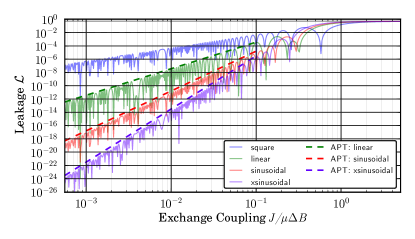
Figure 4: (colour online) A log-log plot of leakage immediately after a gate operation as a function of $J/\mu\Delta B$. Upper bound predictions from adiabatic perturbation theory (dashed lines) are compared to data from simulations (solid traces) for the square (blue), linear (green), sinusoidal (red) and xsinusoidal (purple) adiabatic pulses; demonstrating reasonable agreement.

IV.2 Charge Noise

Charge noise is the result of uncontrolled electromagnetic fields coupling into the control voltages $\varepsilon_{ij}$ of the gates defining the quantum dots; which in turn adds noise to the exchange couplings $J_{ij}$ of equation 7. In this section, we describe our model for charge noise and discuss its effect on our two-qubit gate.

Since charge noise manifests itself in the control voltages $\varepsilon_{ij}$ rather than in $J_{ij}$ directly, we must find an ansatz for $J_{ij}(\varepsilon_{ij})$. This is very difficult to do theoretically; and so we model $J$’s dependence phenomenologically on the basis of known experimental results on single singlet-triplet qubits (recall that singlet-triplet qubits share the same mechanism as our two-qubit gate). In several GaAs singlet-triplet qubit experiments Petta et al. (2005); Foletti et al. (2009); Dial et al. (2013), an exponential ansatz $J(\varepsilon)=J_{0}\exp(\varepsilon/\varepsilon_{D})$ with free parameters $J_{0}$ and $\varepsilon_{D}$ has been found to be a good phenomenological fit to experimental data over a wide range of interesting values of $\varepsilon_{ij}$; and so we adopt it in this work. A more complicated ansatz emerges from perturbation theory Barthel et al. (2012), but due to complex interations of the electrons with the lattice in GaAs experiments, it is not clear whether this ansatz is actually a better description.

While the noise spectrum of $\varepsilon_{ij}$ is difficult to predict theoretically, experimental resultsDial et al. (2013) suggest that the spectrum is reasonably well approximated by a combination of low-frequency pseudo-static components $\bar{\varepsilon}_{ij}$ that do not vary significantly during the gate, and high frequency white-noise components $\tilde{\varepsilon}_{ij}$ that do. We introduce a notation $\hat{\varepsilon}_{ij}$ to refer to the experimentally achieved control voltage, which includes noise atop the theoretically desired value $\varepsilon_{ij}$; i.e. $\hat{\varepsilon}_{ij}=\varepsilon_{ij}+\bar{\varepsilon}_{ij}+\tilde{\varepsilon}_{ij}$. (Dial and collaboratorsDial et al. (2013) also considered a power-law charge noise spectrum which had some advantages over this model, but we do not expect this distinction to qualitatively affect our analysis of the gate and our simpler two-component noise spectrum allows for more straightforward analytical analyses of gate fidelities.)

We model the pseudo-static noise component $\bar{\varepsilon}_{ij}$ to be a random variable normally distributed about zero. These low frequency components give rise to a Gaussian decay in coherence, with a relaxation time of $T_{2}^{*}=\mathchoice{{\hbox{$\displaystyle\sqrt{2\,}$}\lower 0.4pt\hbox{\vrule height=6.44444pt,depth=-5.15558pt}}}{{\hbox{$\textstyle\sqrt{2\,}$}\lower 0.4pt\hbox{\vrule height=6.44444pt,depth=-5.15558pt}}}{{\hbox{$\scriptstyle\sqrt{2\,}$}\lower 0.4pt\hbox{\vrule height=4.51111pt,depth=-3.6089pt}}}{{\hbox{$\scriptscriptstyle\sqrt{2\,}$}\lower 0.4pt\hbox{\vrule height=3.22221pt,depth=-2.57779pt}}}\left(\sigma_{\bar{\varepsilon}}\left|\frac{dJ}{d\varepsilon}\right|\right)^{-1}$, that is reversible using spin echo pulses similar to those used in NMR. The standard deviation of $\bar{\varepsilon}$ ($\sigma_{\bar{\varepsilon}}$) can be determined by fitting $T_{2}^{*}$ times from free induction decay simulations of singlet-triplet qubits to experimentally measured values. The effect of pseudo-static noise on our gate is to shift the average exchange coupling $J_{\textrm{avg}}$ for the gate, causing the two-qubit phase $\int_{0}^{\tau}\left[J_{14}(\hat{\varepsilon}_{14}(t))+J_{23}(\hat{\varepsilon}_{23}(t))\right]dt$ to deviate from its ideal value of $\pi$. With our choice of ansatz for $J$, we find that for any sampled value of $\bar{\varepsilon}$ the two-qubit phase scales like $\pi\exp(\bar{\varepsilon}/\varepsilon_{D})$. This provides the intuition that pseudo-static noise causes an under- or over- accrual of two-qubit phase that is approximately independent of gate time.

The high frequency noise component $\tilde{\varepsilon}_{ij}$ is modelled as Gaussian white noise with mean zero, which means that it is delta correlated $\left<\tilde{\varepsilon}_{ij}(t_{1})\tilde{\varepsilon}_{ij}(t_{2})\right>=D_{ij}\delta(t_{1}-t_{2})$; where $D_{ij}$ is the spectral density of charge fluctuations. The first order correction to the exchange terms in equation 7 due to high frequency noise is $(dJ_{ij}/d\varepsilon_{ij})|_{\varepsilon_{ij}}\tilde{\varepsilon}_{ij}(\bm{\sigma}_{i}\cdot\bm{\sigma}_{j}-II)$. Standard methods can be used to describe the average evolution of the system in this kind of white noise in terms of a master equation Wiseman and Milburn (2010). The resulting Lindblad master equation for the system state $\rho$ is found to be:

$$\dot{\rho}=-i\left[H,\rho\right]+\sum_{\left<i,j\right>}D_{ij}\left|dJ_{ij}/d\varepsilon_{ij}\right|^{2}\mathcal{D}\left[\bm{\sigma}_{i}\cdot\bm{\sigma}_{j}\right],$$ (3)

where $\mathcal{D}\left[O\right]=O^{\dagger}\rho O-\frac{1}{2}\left(\rho O^{\dagger}O+O^{\dagger}O\rho\right)$ is the Lindblad superoperator for some operator $O$. This model describes an irreversible exponential decay in coherence, with a relaxation time of $T_{2}=\left(8D\left|\frac{dJ}{d\varepsilon}\right|^{2}\right)^{-1}$. The spectral density of charge fluctuations $D_{ij}$ can be determined by fitting the results of simulations to experimental $T_{2}$ relaxation times; for example, in Hahn echo experiments.

While this model of charge noise is very simple; we believe it captures the essential details of the noise to which our gate is likely to be most subjected in GaAs semiconductor systems. The model has the nice feature of being completely specified by experimental measurements of $T_{2}$ and $T_{2}^{*}$. An alternative would be to perform simulations with various specified power-law noise spectra; for example, $1/f$ noisePaladino et al. (2014); however, as noted above, we would not expect qualitatively different results from this approach, at least for the performance of a single gate operation.

V Quantifying Gate Performance

We would like to be able to say something about the performance of our two-qubit gate and its resilience against the sources of error introduced in the previous section; which requires us to have a measure of the gate’s performance. While we have already used leakage as a performance indicator in section IV.1, it neither characterises the behaviour of the gate on the logical subspace nor includes the effects of charge noise; and so low leakage does not imply that the desired logical operations have actually occurred. We therefore choose to quantify the performance of our gate by comparing the state of the two-qubit system to some computed ideal state using the entanglement fidelityNielsen and Chuang (2010). The entanglement fidelity is designed to determine whether a gate is accurate for all possible inputs and whether it preserves any initial entanglement with the rest of an imagined quantum computer. It is defined in terms of a thought experiment in which one wants to enact an ideal gate $\bar{U}$ on one half of a maximally entangled state $\left|\Psi_{0}\right>=\frac{1}{\mathchoice{{\hbox{$\displaystyle\sqrt{d\,}$}\lower 0.4pt\hbox{\vrule height=4.8611pt,depth=-3.8889pt}}}{{\hbox{$\textstyle\sqrt{d\,}$}\lower 0.4pt\hbox{\vrule height=4.8611pt,depth=-3.8889pt}}}{{\hbox{$\scriptstyle\sqrt{d\,}$}\lower 0.4pt\hbox{\vrule height=3.40277pt,depth=-2.72223pt}}}{{\hbox{$\scriptscriptstyle\sqrt{d\,}$}\lower 0.4pt\hbox{\vrule height=2.43054pt,depth=-1.94444pt}}}}\sum_{i}\left|\psi_{i}\right>\otimes\left|\psi_{i}\right>$ (where $d$ is the number of logical states, and $d=4$ for a two-qubit gate) to yield $\left|\bar{\Psi}\right>=(\bar{U}\otimes I)\left|\Psi_{0}\right>$. If instead we succeed only in performing $U$, then we yield $\left|\Psi\right>=(U\otimes I)\left|\Psi_{0}\right>$. The entanglement fidelity of $U$ is then just the fidelity between these two states:

$$\mathcal{F}=\left|\left<\bar{\Psi}\big{|}\Psi\right>\right|^{2}.$$

The entanglement fidelity is one if and only if the gate is perfectly implemented, and is less than one for all other operations; with lower values reflecting less accurate implementations of the gate. Among the attractive features of the entanglement fidelity is its simplicity and its close relationship with other measures of gate performance, such as average fidelity Horodecki et al. (1999); Nielsen (2002). Notice that our measure of fidelity assumes that the initial state of the computation is in the logical subspace (and hence $d=4$, rather than $d=6$). Leakage from the logical subspace will result in $\left|\Psi\right>$ living in a larger space, and hence a reduction of entanglement fidelity. The entanglement fidelity can be trivially extended to describe the fidelity of non-unitary (noisy) implementations of the gate.

We are interested only in the performance of the two qubit component of the implemented unitary. Since universal single qubit operations are already possible (see section III.1) and well characterised Petta et al. (2005), we need only a non-trivial two qubit gate to generate a universal set of gates for quantum computation Lloyd (1995). Thus, while in practice our protocol produces a CPHASE gate along with some known single qubit rotations (as described in section III.2), it would not be necessary in some experimental implementations to correct them immediately after each gate application; and if it were, these gates can be echoed away by a protocol such as the one in Klinovaja et al.Klinovaja et al. (2012). Consequently, we compute the entanglement fidelity of our gate assuming that the optimal single qubit corrections have been perfectly applied. In practice this means that we compare our gate to a constructed ideal unitary $\bar{U}$ that maintains the ideal two-qubit phase while also including whatever single qubit z-rotations we find in the simulation of our gate. This corresponds to an ansatz $\bar{U}=e^{i\phi_{II}}e^{i\phi_{ZI}\tilde{\sigma}_{z}^{1}}e^{i\phi_{IZ}\tilde{\sigma}_{z}^{2}}e^{i\phi_{ZZ}\tilde{\sigma}_{z}^{1}\tilde{\sigma}_{z}^{2}}$ with global and single-qubit phases $\phi_{II}$, $\phi_{IZ}$ and $\phi_{ZI}$ extracted from simulations, and the two-qubit phase $\phi_{ZZ}$ set to $\pi$. There are some subtleties to this process which we discuss in the supplementary material.

The simplicity of our two singlet-triplet qubit model allows us to gain some intuition about the entanglement fidelity by considering the analytic solution for fidelity in terms of the leakage at the end of the gate $\mathcal{L}_{0}$ and the parameter $\Delta=\phi_{ZZ}-\bar{\phi}_{ZZ}$, where $\phi_{ZZ}$ and $\bar{\phi}_{ZZ}=\pi$ are the extracted and ideal two qubit phases respectively. Note that $\Delta$ characterises any under- or over- accrual of two-qubit phase acquired during the gate operation. We show in the supplementary material that the entanglement fidelity $\mathcal{F}$ at the end of the gate is:

$$\mathcal{F} =\frac{1}{2}\left(1+\mathchoice{{\hbox{$\displaystyle\sqrt{1-2\mathcal{L}_{0}\,}$}\lower 0.4pt\hbox{\vrule height=6.83331pt,depth=-5.46667pt}}}{{\hbox{$\textstyle\sqrt{1-2\mathcal{L}_{0}\,}$}\lower 0.4pt\hbox{\vrule height=6.83331pt,depth=-5.46667pt}}}{{\hbox{$\scriptstyle\sqrt{1-2\mathcal{L}_{0}\,}$}\lower 0.4pt\hbox{\vrule height=4.78333pt,depth=-3.82668pt}}}{{\hbox{$\scriptscriptstyle\sqrt{1-2\mathcal{L}_{0}\,}$}\lower 0.4pt\hbox{\vrule height=3.41666pt,depth=-2.73334pt}}}\cos\left(2\Delta\right)-\mathcal{L}_{0}\right)$$ (4)

$$=1-\mathcal{L}_{0}-\Delta^{2}+\mathcal{O}(\mathcal{L}_{0}^{2})+\mathcal{O}(\mathcal{L}_{0}\Delta^{2})+\mathcal{O}(\Delta^{4}).$$ (5)

Perfect gate implementations will have $\Delta=0$, whereas in the presence of charge noise it will assume non-zero values since $\phi_{ZZ}\simeq\int_{0}^{\tau}\left[J_{14}(t)+J_{23}(t)\right]dt$.

Our charge noise model of section IV.2 allows us to make some more quantitative statements about $\Delta$. Consider a square pulse for simplicity (adiabatic pulses are not expected to lead to qualitatively different results) with first order noise perturbations, $J(t)=J_{\textrm{avg}}+(\bar{\varepsilon}+\tilde{\varepsilon})(dJ/d\varepsilon)|_{J(\varepsilon)=J_{\mathrm{avg}}}$ where $\bar{\varepsilon}$ and $\tilde{\varepsilon}$ are the pseudo-static and high frequency potential fluctuations caused by charge noise (see section IV.2). The phase error $\Delta$ is then:

$$\Delta=\frac{\pi}{J_{\mathrm{avg}}}\left.\frac{dJ}{d\varepsilon}\right|_{J=J_{\mathrm{avg}}}(\bar{\varepsilon}+\tilde{\varepsilon})_{\mathrm{avg}}$$

where $(\bar{\varepsilon}+\tilde{\varepsilon})_{\mathrm{avg}}=\int_{0}^{\tau}\left[(\bar{\varepsilon}+\tilde{\varepsilon})/\tau\right]dt$ is the average charge fluctuation during the operation of the gate. Our noise model posits that $\bar{\varepsilon}$ and $\tilde{\varepsilon}$ are both independent and Gaussian distributed; which allows us to easily calculate the statistical properties of $(\bar{\varepsilon}+\tilde{\varepsilon})_{\mathrm{avg}}$: $\left<(\bar{\varepsilon}+\tilde{\varepsilon})_{\mathrm{avg}}\right>=0$ and $\left<(\bar{\varepsilon}+\tilde{\varepsilon})_{\mathrm{avg}}^{2}\right>=\sigma_{\bar{\varepsilon}}^{2}+D/\tau$. While different charge spectra beyond our model would lead to different time dependences for $\left<(\bar{\varepsilon}+\tilde{\varepsilon})_{\mathrm{avg}}^{2}\right>$, it would always be qualitatively true that non-pseudo-static noise averages out over long enough time scales. This implies the statistical properties of $\Delta$:

$$\left<\Delta\right> = 0$$

$$\left<\Delta^{2}\right> = \frac{\pi^{2}}{J_{\mathrm{avg}}^{2}}\left.\frac{dJ}{d\varepsilon}\right|_{J=J_{\mathrm{avg}}}^{2}\left(\sigma_{\bar{\varepsilon}}^{2}+D/\tau\right).$$

If we further assume the exponential ansatz $J\simeq J_{0}\exp(\varepsilon/\varepsilon_{D})$ we obtain a particularly simple estimate of the expected entanglement fidelity $\left<\mathcal{F}\right>$:

$$\left\langle\mathcal{F}\right\rangle\simeq 1-\mathcal{L}_{0}-\pi^{2}\frac{\sigma_{\bar{\varepsilon}}^{2}+D/\tau}{\varepsilon_{D}^{2}}.$$ (6)

This formula affords us the important intuition that one is in principle able to maximise the fidelity of our gate by choosing sufficiently long gate times; at which point fidelity will be limited by a pseudo-static noise floor that also determines the fidelity of single-qubit operations. This is evident because both leakage and the effect of high frequency noise are monotonically decreasing functions of the choice of gate time; and pseudo-static noise contributions are constant. The leakage $\mathcal{L}_{0}$ due to the pulse scales as $(\tau\Delta B)^{-c}$ for some $c$ that depends on the adiabaticity of the pulse (as shown in section IV.1). Additional leakage contributions arise from high frequency noise, at a rate $4D|dJ/d\varepsilon|^{2}$ predicted by the master equation (3), and hence a contribution to $\mathcal{L}_{0}$ proportional to $D/(\tau\varepsilon_{D}^{2})$. Since all sources of fidelity dimunition apart from pseudo-static noise decrease as gate time increases, pseudo-static noise will dominate at sufficiently long gate times; after which the fidelity becomes roughly independent of gate time. In the limit that leakage is no longer the dominant noise contribution, equation 6 reduces to the fidelity relation for a single qubit gate; implying that our gate would operate with essentially identical fidelity as single qubit operations.

Although we have largely neglected the effects of Overhauser field fluctuations on our simulations, since they are expected to be less significant than charge noise in the usual regime of operation, it would be straightforward to include them in this kind of analysis. The main effect of these fluctuations is to implement random single qubit unitaries during the gate; which would result in a reduction of gate fidelity proportional to the variance of the field fluctuation.

VI Simulations

(a)

(b)

(c)

(d)

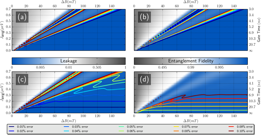
Figure 5: (colour online) Simulated leakage and entanglement fidelity immediately after a single two-qubit gate operation as a function of $J_{\mathrm{avg}}$ and $\Delta B$; with gate time corresponding to each labelled $J_{\mathrm{avg}}$ shown on the far right axes. Subplots (a) and (c) show the leakage results with and without charge noise respectively; and subplots (b) and (d) show the entanglement fidelity results with and without charge noise respectively. The colour maps for leakage and entanglement fidelity are shown in the corresponding column, and are chosen such that comparable colours indicate comparable errors. The colour maps are white at $1\%$ error; with larger error shown in shades of grey; and lesser error in shades of blue. Contours corresponding to 0.01%-0.10% error are drawn at 0.01% intervals.

We are left now only to demonstrate the performance of our two singlet-triplet gate in simulations. For the purposes of this section, we integrate the time dependent Heisenberg Hamiltonian (with and without the Lindblad terms) as described in equations 7 and 3. One might worry that the weak tunnelling approximation described in section II might lead to appreciable errors; but simulations of a full Hubbard model generated indistinguishable results in all of our tests. We have chosen to consider a case where $J_{14}=0$, and henceforth $J=J_{23}$, because we expect a linear arrangement of quantum dots to be more accessible to experimental implementation. Simulating a square configuration is a trivial extension that does not alter the physics; indeed it improves the gate speed for any given leakage error, and reduces the complexity of the unwanted single qubit gates (refer to the supplementary material for more information). For reasons mentioned in section IV.1, we have chosen to use the sinusoidal adiabatic pulse in these simulations.

All of the parameters used in these simulations have been chosen with current experiments in mind. The average background magnetic field $B_{0}$ is maintained as the dominant energy scale, and set to be $200\,mT$. As described in section IV.2, simulations of our gate require us to choose an ansatz for $J(\varepsilon$); the details of which are not important provided that the dependence matches closely phenomenological results. In these simulations we use $J(\varepsilon)=J_{0}\exp(\varepsilon/\varepsilon_{D})$, with the free parameters $J_{0}$ and $\varepsilon_{D}$ chosen to roughly match the experimental results of Dial and collaborators Dial et al. (2013). In simulations we add a very small negative constant offset to allow for $J(\varepsilon)$ to be exactly zero, which does not significantly affect the results. Also following the prescription of section IV.2, we calibrated the noise parameters $\sigma_{\bar{\varepsilon}}$ and $D$ such that the $T_{2}^{*}$ and $T_{2}$ times in simulations of single-qubit gates were somewhat typicalDial et al. (2013); specifically, we calibrated $\sigma_{\bar{\varepsilon}}$ and $D$ such that $T_{2}^{*}\approx 100\,ns$ and $T_{2}\approx 1\,\mu s$. We summarise our choice of parameters in table 2.

Parameter	Value
Magnetic Field:
$B_{0}$	$200\,mT$
Noise:
$\sigma_{\bar{\varepsilon}}$	$10.3\,\mu V$
$D$	$100\,\mu V^{2}\,ns$
Exponential Ansatz:
$J_{0}$	$-82.7\,\mu eV\,(\approx 20GHz$)
$\varepsilon_{D}$	$0.35\,mV$

Table 2: Model parameters kept constant while exploring $J$ and $\Delta B$. The global magnetic field is nominal. The noise parameters $\sigma_{\bar{\varepsilon}}$ and $D$ were calibrated by respectively matching somewhat typical values of $T_{2}^{*}$ and $T_{2}$ from experimentDial et al. (2013). The parameters for the exponential ansatz $J(\varepsilon)=J_{0}\exp(\varepsilon/\varepsilon_{D})$ were chosen to roughly match the experimental results of Dial and collaborators Dial et al. (2013).

In figure 5 we plot leakage with and without charge noise (5a and 5c respectively), and entanglement fidelity with and without noise (5b and 5d respectively), at the end of a single two-qubit gate operation as a function of the average exchange coupling $J_{\mathrm{avg}}$ and inter-qubit magnetic field gradient $\Delta B$. The gate time corresponding to each value of $J_{\mathrm{avg}}$ is labelled on the rightmost axes. We use a segmented colour map which goes through white at 1% error; with blue toward 0% and dark grey toward 100%. Contours corresponding to 0.01%-0.10% error are drawn at 0.01% intervals; corresponding to the regime in which fault-tolerant computing starts to become feasible (typically $10^{-2}-10^{-4}$ )Gottesman (2007). The positions of the contours on both the leakage and fidelity plots roughly correspond, because $\mathcal{F}\approx 1-\mathcal{L}_{0}$ (see section V).

The simulations confirm several important qualities of our gate. The radial nature of the contours from the origin indicates that our gate’s leakage is largely predicted by the ratio $J_{\mathrm{avg}}/\mu\Delta B$, as described in section IV.1. We also observe the qualitative features of anticipated in section V: that charge noise causes the entanglement fidelity to decrease even more quickly than leakage increases due to its being sensitive to phases on the logical subspace (seen in 6); that leakage ceases to be the dominant source of error (for any given fidelity) at long enough gate times; and that fidelity increases approximately hyperbolically with gate time (or equivalently, decreases linearly with $J_{\mathrm{avg}}$).

By way of ballpark numbers, we find that our two-qubit gate has fidelities in excess of $\sim 99.9\%$ for gate times longer than around $7\,ns$ and magnetic field gradients of around $80\,mT$. In this regime, leakage is no longer the dominant source of noise; and gate fidelities are affected by noise in essentially the same way as single qubit gates, as described in section V. On this basis, we feel that our gate may be well suited for quantum computation using singlet-triplet qubits.

VII Discussion

In this paper we have analysed the performance of an exchange-based two-qubit gate for singlet-triplet qubits. Our approach uses a magnetic field gradient to suppress spin-flip transitions that would otherwise lead to leakage errors. We have shown that adiabatic pulses can reduce the leakage probability by several orders of magnitude. We have also investigated the effect of charge noise on the performance of our gate; showing that, by running the gate sufficiently slowly, it is possible to achieve entanglement fidelities that are comparable to those of single qubit operations. In this limit, we showed that the performance is limited by low frequency charge noise. Two-qubit gate simulations demonstrated that this regime can be reached using realistic exchange couplings and magnetic field gradients.

The two-qubit gate we have described works whenever there is an effective exchange coupling between the qubits. This could be a direct exchange coupling (as we have envisaged here), or an indirect coupling through an intermediate dot which has recently been shown to generate an effective exchange interaction Mehl et al. (2014).

The approach of energetically suppressing spin-flip transitions in order to implement two-qubit gates using exchange coupling has application in other qubit architectures; for example, we used a similar approach in our proposal for two-qubit gates for the resonant-exchange qubit Doherty and Wardrop (2013). We anticipate that the use of adiabatic pulses will greatly reduce leakage in that scheme also.

Supplementary A Analytically solving for the eigen-energies of a two singlet-triplet qubit system

In the paper we claimed that it was possible to derive exact solutions the eigen- energies and states of the Hamiltonian:

$$H(t)=\mu\sum_{n=1}^{N}B_{n}(t)\sigma_{z}^{n}+\frac{1}{4}\sum_{\left<i,j\right>}J_{ij}(t)(\bm{\sigma}^{i}\cdot\bm{\sigma}^{j}-I),$$ (7)

where $J_{14}$ and $J_{23}$ are the only non-zero exchange couplings. We do so in the following for the case were $J_{14}=0$ (the “linear” configuration), and where both $J_{14}$ and $J_{23}$ are non-zero; which has a special case $J_{14}=J_{23}$ (the “square” configuration).

A.1 Simple two-level system

Consider first a two-level system with Hamiltonian:

$$H=\frac{\Delta B}{2}\sigma_{z}+\frac{J}{2}\sigma_{x},$$

where we consider the spin states to be the eigenstates of $\sigma_{z}$, and where in principle each parameter can be time dependent. This Hamiltonian has eigen-energies:

$$E_{\pm} = \pm\frac{\Delta B}{2}\mathchoice{{\hbox{$\displaystyle\sqrt{1+\xi^{2}\,}$}\lower 0.4pt\hbox{\vrule height=8.74889pt,depth=-6.99915pt}}}{{\hbox{$\textstyle\sqrt{1+\xi^{2}\,}$}\lower 0.4pt\hbox{\vrule height=8.74889pt,depth=-6.99915pt}}}{{\hbox{$\scriptstyle\sqrt{1+\xi^{2}\,}$}\lower 0.4pt\hbox{\vrule height=6.14998pt,depth=-4.92001pt}}}{{\hbox{$\scriptscriptstyle\sqrt{1+\xi^{2}\,}$}\lower 0.4pt\hbox{\vrule height=4.7611pt,depth=-3.8089pt}}},$$

with $\xi=\frac{J}{\Delta B}$. The corresponding eigenstates are given by:

$$\left|\psi\right>_{+} = \left|\uparrow\right>+(\mathchoice{{\hbox{$\displaystyle\sqrt{1+\xi^{2}\,}$}\lower 0.4pt\hbox{\vrule height=8.74889pt,depth=-6.99915pt}}}{{\hbox{$\textstyle\sqrt{1+\xi^{2}\,}$}\lower 0.4pt\hbox{\vrule height=8.74889pt,depth=-6.99915pt}}}{{\hbox{$\scriptstyle\sqrt{1+\xi^{2}\,}$}\lower 0.4pt\hbox{\vrule height=6.14998pt,depth=-4.92001pt}}}{{\hbox{$\scriptscriptstyle\sqrt{1+\xi^{2}\,}$}\lower 0.4pt\hbox{\vrule height=4.7611pt,depth=-3.8089pt}}}-1)/\xi\left|\downarrow\right>$$

$$\left|\psi\right>_{-} = \left|\uparrow\right>-(\mathchoice{{\hbox{$\displaystyle\sqrt{1+\xi^{2}\,}$}\lower 0.4pt\hbox{\vrule height=8.74889pt,depth=-6.99915pt}}}{{\hbox{$\textstyle\sqrt{1+\xi^{2}\,}$}\lower 0.4pt\hbox{\vrule height=8.74889pt,depth=-6.99915pt}}}{{\hbox{$\scriptstyle\sqrt{1+\xi^{2}\,}$}\lower 0.4pt\hbox{\vrule height=6.14998pt,depth=-4.92001pt}}}{{\hbox{$\scriptscriptstyle\sqrt{1+\xi^{2}\,}$}\lower 0.4pt\hbox{\vrule height=4.7611pt,depth=-3.8089pt}}}+1)/\xi\left|\downarrow\right>.$$

In the following sections we will break up more complicated Hamiltonians into two-level systems, and solve them by comparing them to these results.

A.2 Singlet-triplet qubit system

We derive the solutions for a singlet-triplet qubit system; before providing solutions for two singlet-triplet systems in subsequent sections. The Hamiltonian for single singlet-triplet qubit system is:

$$H=\mu B_{1}\sigma_{z}^{1}+\mu B_{2}\sigma_{z}^{2}+\frac{J}{4}(\bm{\sigma}^{1}\cdot\bm{\sigma}^{2}-I)\,.$$

The effect of the exchange coupling term is to lower the singlet state compared to the triplet states. The $\sum S_{z}=1$ and $\sum S_{z}=-1$ states $\left|\uparrow\uparrow\right>$ and $\left|\downarrow\downarrow\right>$ are unaffected by the exchange coupling; and so their eigen-energies are $\mu(B_{1}+B_{2})$ and $-\mu(B_{1}+B_{2})$ respectively. The effect of the Hamiltonian on the remaining singlet and triplet states with $\sum S_{z}=0$, which corresponds to the logical subspace as described in the main text, can be written as:

$$\left(\begin{array}[]{cc}\mu\Delta_{12}-\frac{J}{2}&\frac{J}{2}\\ \frac{J}{2}&-\mu\Delta_{12}-\frac{J}{2}\end{array}\right)\left(\begin{array}[]{c}\left|\uparrow\downarrow\right>\\ \left|\downarrow\uparrow\right>\end{array}\right),$$

with $\Delta_{12}=B_{1}-B_{2}$. By comparison with the simple two-level system in the previous section, we find that the eigen-energies of the states which adiabatically conform to the logical spin basis states $\left|\uparrow\downarrow\right>$ and $\left|\downarrow\uparrow\right>$ in the limit that $J=0$ are:

$$E_{\uparrow\downarrow} = \mu\Delta_{12}\mathchoice{{\hbox{$\displaystyle\sqrt{1+\xi^{2}\,}$}\lower 0.4pt\hbox{\vrule height=8.74889pt,depth=-6.99915pt}}}{{\hbox{$\textstyle\sqrt{1+\xi^{2}\,}$}\lower 0.4pt\hbox{\vrule height=8.74889pt,depth=-6.99915pt}}}{{\hbox{$\scriptstyle\sqrt{1+\xi^{2}\,}$}\lower 0.4pt\hbox{\vrule height=6.14998pt,depth=-4.92001pt}}}{{\hbox{$\scriptscriptstyle\sqrt{1+\xi^{2}\,}$}\lower 0.4pt\hbox{\vrule height=4.7611pt,depth=-3.8089pt}}}-\frac{J}{2}$$

$$E_{\downarrow\uparrow} = -\mu\Delta_{12}\mathchoice{{\hbox{$\displaystyle\sqrt{1+\xi^{2}\,}$}\lower 0.4pt\hbox{\vrule height=8.74889pt,depth=-6.99915pt}}}{{\hbox{$\textstyle\sqrt{1+\xi^{2}\,}$}\lower 0.4pt\hbox{\vrule height=8.74889pt,depth=-6.99915pt}}}{{\hbox{$\scriptstyle\sqrt{1+\xi^{2}\,}$}\lower 0.4pt\hbox{\vrule height=6.14998pt,depth=-4.92001pt}}}{{\hbox{$\scriptscriptstyle\sqrt{1+\xi^{2}\,}$}\lower 0.4pt\hbox{\vrule height=4.7611pt,depth=-3.8089pt}}}-\frac{J}{2}$$

with $\xi=J/\mu\Delta_{12}$. The eigenstates will have the same form as those of the previous section; where $\left|\uparrow\right>\mapsto\left|\uparrow\downarrow\right>$ and $\left|\downarrow\right>\mapsto\left|\downarrow\uparrow\right>$.

A.3 Linear configuration for two singlet-triplet qubits

We now consider the energy spectrum of a two singlet-triplet qubit system in the linear configuration; that is, with exchange coupling only between the second and third quantum dots. The Hamiltonian for this system is given by:

$$H=\mu\sum_{n=1}^{4}B_{n}\sigma_{z}^{n}+\frac{1}{4}J_{23}(\bm{\sigma}^{2}\cdot\bm{\sigma}^{3}-I).$$

As in the paper, we imagine a large global magnetic field; making the spin basis a natural one. Moreover, since we are not going to be considering the possibility of spin-flip, only system states with like total $\sum S_{Z}$ can communicate. Grouping the states by like $\sum S_{z}$, we find 5 different groups with $\sum S_{z}=0,\pm 1,\pm 2$. By comparision to the previous section, it is clear that only eigenstates that have different spin states for quantum dots 2 and 3 will be coupled by the interaction. This forms a series of two level coherences; i.e. $\left|\uparrow\uparrow,\downarrow\uparrow\right>\rightleftarrows\left|\uparrow\downarrow,\uparrow\uparrow\right>;\,\left|\uparrow\uparrow,\downarrow\downarrow\right>\rightleftarrows\left|\uparrow\downarrow,\uparrow\downarrow\right>$; etc. We use the same magnetic field basis used in the paper: the global background magnetic field $B_{0}=\frac{1}{4}\sum_{n}B_{n}$, the inter-qubit gradient $\Delta B=\frac{1}{2}\left(B_{1}+B_{2}-B_{3}-B_{4}\right)$, and the intra-qubit gradients $\Delta_{12}$ and $\Delta_{34}$ with $\Delta_{ij}=B_{i}-B_{j}$.

By applying a similar analysis as that in the previous section, we tabulate the energies for the states which adiabatically conform to the spin states below.

$$\begin{array}[]{ccc}\mathbf{m_{z}}&\textbf{Eigenstate}&\textbf{Energy}\\ 2&\left|\uparrow\uparrow\uparrow\uparrow\right>&4\mu B_{0}\\ 1&\left|\uparrow\uparrow\uparrow\downarrow\right>&2\mu B_{0}+\mu\Delta B+\mu\Delta_{34}\\ 1&\left|\uparrow\uparrow\downarrow\uparrow\right>&2\mu B_{0}+\frac{1}{2}\mu(\Delta_{12}-\Delta_{34})-\frac{1}{2}J_{23}+\mathchoice{{\hbox{$\displaystyle\sqrt{\left(\mu\Delta B-\frac{1}{2}\mu(\Delta_{12}+\Delta_{34})\right)^{2}+\frac{1}{4}J_{23}^{2}\,}$}\lower 0.4pt\hbox{\vrule height=9.66666pt,depth=-7.73337pt}}}{{\hbox{$\textstyle\sqrt{\left(\mu\Delta B-\frac{1}{2}\mu(\Delta_{12}+\Delta_{34})\right)^{2}+\frac{1}{4}J_{23}^{2}\,}$}\lower 0.4pt\hbox{\vrule height=9.30444pt,depth=-7.44359pt}}}{{\hbox{$\scriptstyle\sqrt{\left(\mu\Delta B-\frac{1}{2}\mu(\Delta_{12}+\Delta_{34})\right)^{2}+\frac{1}{4}J_{23}^{2}\,}$}\lower 0.4pt\hbox{\vrule height=6.53888pt,depth=-5.23112pt}}}{{\hbox{$\scriptscriptstyle\sqrt{\left(\mu\Delta B-\frac{1}{2}\mu(\Delta_{12}+\Delta_{34})\right)^{2}+\frac{1}{4}J_{23}^{2}\,}$}\lower 0.4pt\hbox{\vrule height=5.03888pt,depth=-4.03113pt}}}\\ 1&\left|\uparrow\downarrow\uparrow\uparrow\right>&2\mu B_{0}+\frac{1}{2}\mu(\Delta_{12}-\Delta_{34})-\frac{1}{2}J_{23}-\mathchoice{{\hbox{$\displaystyle\sqrt{\left(\mu\Delta B-\frac{1}{2}\mu(\Delta_{12}+\Delta_{34})\right)^{2}+\frac{1}{4}J_{23}^{2}\,}$}\lower 0.4pt\hbox{\vrule height=9.66666pt,depth=-7.73337pt}}}{{\hbox{$\textstyle\sqrt{\left(\mu\Delta B-\frac{1}{2}\mu(\Delta_{12}+\Delta_{34})\right)^{2}+\frac{1}{4}J_{23}^{2}\,}$}\lower 0.4pt\hbox{\vrule height=9.30444pt,depth=-7.44359pt}}}{{\hbox{$\scriptstyle\sqrt{\left(\mu\Delta B-\frac{1}{2}\mu(\Delta_{12}+\Delta_{34})\right)^{2}+\frac{1}{4}J_{23}^{2}\,}$}\lower 0.4pt\hbox{\vrule height=6.53888pt,depth=-5.23112pt}}}{{\hbox{$\scriptscriptstyle\sqrt{\left(\mu\Delta B-\frac{1}{2}\mu(\Delta_{12}+\Delta_{34})\right)^{2}+\frac{1}{4}J_{23}^{2}\,}$}\lower 0.4pt\hbox{\vrule height=5.03888pt,depth=-4.03113pt}}}\\ 1&\left|\downarrow\uparrow\uparrow\uparrow\right>&2\mu B_{0}-\mu\Delta B-\mu\Delta_{12}\\ 0&\left|\uparrow\uparrow\downarrow\downarrow\right>&\mu\Delta B+\frac{1}{2}\mu(\Delta_{12}+\Delta_{34})-\frac{1}{2}J_{23}+\mathchoice{{\hbox{$\displaystyle\sqrt{\left(\mu\Delta B-\frac{1}{2}\mu(\Delta_{12}+\Delta_{34})\right)^{2}+\frac{1}{4}J_{23}^{2}\,}$}\lower 0.4pt\hbox{\vrule height=9.66666pt,depth=-7.73337pt}}}{{\hbox{$\textstyle\sqrt{\left(\mu\Delta B-\frac{1}{2}\mu(\Delta_{12}+\Delta_{34})\right)^{2}+\frac{1}{4}J_{23}^{2}\,}$}\lower 0.4pt\hbox{\vrule height=9.30444pt,depth=-7.44359pt}}}{{\hbox{$\scriptstyle\sqrt{\left(\mu\Delta B-\frac{1}{2}\mu(\Delta_{12}+\Delta_{34})\right)^{2}+\frac{1}{4}J_{23}^{2}\,}$}\lower 0.4pt\hbox{\vrule height=6.53888pt,depth=-5.23112pt}}}{{\hbox{$\scriptscriptstyle\sqrt{\left(\mu\Delta B-\frac{1}{2}\mu(\Delta_{12}+\Delta_{34})\right)^{2}+\frac{1}{4}J_{23}^{2}\,}$}\lower 0.4pt\hbox{\vrule height=5.03888pt,depth=-4.03113pt}}}\\ 0&\left|\uparrow\downarrow\uparrow\downarrow\right>&\mu\Delta B+\frac{1}{2}\mu(\Delta_{12}+\Delta_{34})-\frac{1}{2}J_{23}-\mathchoice{{\hbox{$\displaystyle\sqrt{\left(\mu\Delta B-\frac{1}{2}\mu(\Delta_{12}+\Delta_{34})\right)^{2}+\frac{1}{4}J_{23}^{2}\,}$}\lower 0.4pt\hbox{\vrule height=9.66666pt,depth=-7.73337pt}}}{{\hbox{$\textstyle\sqrt{\left(\mu\Delta B-\frac{1}{2}\mu(\Delta_{12}+\Delta_{34})\right)^{2}+\frac{1}{4}J_{23}^{2}\,}$}\lower 0.4pt\hbox{\vrule height=9.30444pt,depth=-7.44359pt}}}{{\hbox{$\scriptstyle\sqrt{\left(\mu\Delta B-\frac{1}{2}\mu(\Delta_{12}+\Delta_{34})\right)^{2}+\frac{1}{4}J_{23}^{2}\,}$}\lower 0.4pt\hbox{\vrule height=6.53888pt,depth=-5.23112pt}}}{{\hbox{$\scriptscriptstyle\sqrt{\left(\mu\Delta B-\frac{1}{2}\mu(\Delta_{12}+\Delta_{34})\right)^{2}+\frac{1}{4}J_{23}^{2}\,}$}\lower 0.4pt\hbox{\vrule height=5.03888pt,depth=-4.03113pt}}}\\ 0&\left|\uparrow\downarrow\downarrow\uparrow\right>&\mu\Delta_{12}-\mu\Delta_{34}\\ 0&\left|\downarrow\uparrow\uparrow\downarrow\right>&-\mu\Delta_{12}+\mu\Delta_{34}\\ 0&\left|\downarrow\uparrow\downarrow\uparrow\right>&-\mu\Delta B-\frac{1}{2}\mu(\Delta_{12}+\Delta_{34})-\frac{1}{2}\,J_{23}+\mathchoice{{\hbox{$\displaystyle\sqrt{\left(\mu\Delta B-\frac{1}{2}\mu(\Delta_{12}+\Delta_{34})\right)^{2}+\frac{1}{4}J_{23}^{2}\,}$}\lower 0.4pt\hbox{\vrule height=9.66666pt,depth=-7.73337pt}}}{{\hbox{$\textstyle\sqrt{\left(\mu\Delta B-\frac{1}{2}\mu(\Delta_{12}+\Delta_{34})\right)^{2}+\frac{1}{4}J_{23}^{2}\,}$}\lower 0.4pt\hbox{\vrule height=9.30444pt,depth=-7.44359pt}}}{{\hbox{$\scriptstyle\sqrt{\left(\mu\Delta B-\frac{1}{2}\mu(\Delta_{12}+\Delta_{34})\right)^{2}+\frac{1}{4}J_{23}^{2}\,}$}\lower 0.4pt\hbox{\vrule height=6.53888pt,depth=-5.23112pt}}}{{\hbox{$\scriptscriptstyle\sqrt{\left(\mu\Delta B-\frac{1}{2}\mu(\Delta_{12}+\Delta_{34})\right)^{2}+\frac{1}{4}J_{23}^{2}\,}$}\lower 0.4pt\hbox{\vrule height=5.03888pt,depth=-4.03113pt}}}\\ 0&\left|\downarrow\downarrow\uparrow\uparrow\right>&-\mu\Delta B-\frac{1}{2}\mu(\Delta_{12}+\Delta_{34})-\frac{1}{2}\,J_{23}-\mathchoice{{\hbox{$\displaystyle\sqrt{\left(\mu\Delta B-\frac{1}{2}\mu(\Delta_{12}+\Delta_{34})\right)^{2}+\frac{1}{4}J_{23}^{2}\,}$}\lower 0.4pt\hbox{\vrule height=9.66666pt,depth=-7.73337pt}}}{{\hbox{$\textstyle\sqrt{\left(\mu\Delta B-\frac{1}{2}\mu(\Delta_{12}+\Delta_{34})\right)^{2}+\frac{1}{4}J_{23}^{2}\,}$}\lower 0.4pt\hbox{\vrule height=9.30444pt,depth=-7.44359pt}}}{{\hbox{$\scriptstyle\sqrt{\left(\mu\Delta B-\frac{1}{2}\mu(\Delta_{12}+\Delta_{34})\right)^{2}+\frac{1}{4}J_{23}^{2}\,}$}\lower 0.4pt\hbox{\vrule height=6.53888pt,depth=-5.23112pt}}}{{\hbox{$\scriptscriptstyle\sqrt{\left(\mu\Delta B-\frac{1}{2}\mu(\Delta_{12}+\Delta_{34})\right)^{2}+\frac{1}{4}J_{23}^{2}\,}$}\lower 0.4pt\hbox{\vrule height=5.03888pt,depth=-4.03113pt}}}\\ -1&\left|\uparrow\downarrow\downarrow\downarrow\right>&-2\mu B_{0}+\mu\Delta B+\mu\Delta_{12}\\ -1&\left|\downarrow\uparrow\downarrow\downarrow\right>&-2\mu B_{0}-\frac{1}{2}\mu(\Delta_{12}-\Delta_{34})-\frac{1}{2}\,J_{23}+\mathchoice{{\hbox{$\displaystyle\sqrt{\left(\mu\Delta B-\frac{1}{2}\mu(\Delta_{12}+\Delta_{34})\right)^{2}+\frac{1}{4}J_{23}^{2}\,}$}\lower 0.4pt\hbox{\vrule height=9.66666pt,depth=-7.73337pt}}}{{\hbox{$\textstyle\sqrt{\left(\mu\Delta B-\frac{1}{2}\mu(\Delta_{12}+\Delta_{34})\right)^{2}+\frac{1}{4}J_{23}^{2}\,}$}\lower 0.4pt\hbox{\vrule height=9.30444pt,depth=-7.44359pt}}}{{\hbox{$\scriptstyle\sqrt{\left(\mu\Delta B-\frac{1}{2}\mu(\Delta_{12}+\Delta_{34})\right)^{2}+\frac{1}{4}J_{23}^{2}\,}$}\lower 0.4pt\hbox{\vrule height=6.53888pt,depth=-5.23112pt}}}{{\hbox{$\scriptscriptstyle\sqrt{\left(\mu\Delta B-\frac{1}{2}\mu(\Delta_{12}+\Delta_{34})\right)^{2}+\frac{1}{4}J_{23}^{2}\,}$}\lower 0.4pt\hbox{\vrule height=5.03888pt,depth=-4.03113pt}}}\\ -1&\left|\downarrow\downarrow\uparrow\downarrow\right>&-2\mu B_{0}-\frac{1}{2}\mu(\Delta_{12}-\Delta_{34})-\frac{1}{2}\,J_{23}-\mathchoice{{\hbox{$\displaystyle\sqrt{\left(\mu\Delta B-\frac{1}{2}\mu(\Delta_{12}+\Delta_{34})\right)^{2}+\frac{1}{4}J_{23}^{2}\,}$}\lower 0.4pt\hbox{\vrule height=9.66666pt,depth=-7.73337pt}}}{{\hbox{$\textstyle\sqrt{\left(\mu\Delta B-\frac{1}{2}\mu(\Delta_{12}+\Delta_{34})\right)^{2}+\frac{1}{4}J_{23}^{2}\,}$}\lower 0.4pt\hbox{\vrule height=9.30444pt,depth=-7.44359pt}}}{{\hbox{$\scriptstyle\sqrt{\left(\mu\Delta B-\frac{1}{2}\mu(\Delta_{12}+\Delta_{34})\right)^{2}+\frac{1}{4}J_{23}^{2}\,}$}\lower 0.4pt\hbox{\vrule height=6.53888pt,depth=-5.23112pt}}}{{\hbox{$\scriptscriptstyle\sqrt{\left(\mu\Delta B-\frac{1}{2}\mu(\Delta_{12}+\Delta_{34})\right)^{2}+\frac{1}{4}J_{23}^{2}\,}$}\lower 0.4pt\hbox{\vrule height=5.03888pt,depth=-4.03113pt}}}\\ -1&\left|\downarrow\downarrow\downarrow\uparrow\right>&-2\mu B_{0}-\mu\Delta B-\mu\Delta_{34}\\ -2&\left|\downarrow\downarrow\downarrow\downarrow\right>&-4\mu B_{0}\end{array}$$

A.4 Non-linear configuration for two singlet-triplet qubits

We now consider the more general configuration in which both $J_{14}$ and $J_{23}$ are non-zero; and present an analogous table of eigenvalues (as above). In the case where $J_{14}=J_{23}$ we form what we call the square configuration. Since the two exchange couplings are acting identically in a disjoint system (since $J_{12}$ and $J_{34}$ are turned off); these eigenvalues follow immediately from those above.

$$\begin{array}[]{ccc}\mathbf{m_{z}}&\textbf{Eigenstate}&\textbf{Energy}\\ 2&\left|\uparrow\uparrow\uparrow\uparrow\right>&4\mu B_{0}\\ 1&\left|\uparrow\uparrow\uparrow\downarrow\right>&2\mu B_{0}-\frac{1}{2}\mu(\Delta_{12}-\Delta_{34})-\frac{1}{2}J_{14}+\mathchoice{{\hbox{$\displaystyle\sqrt{\left(\mu\Delta B+\frac{1}{2}\mu(\Delta_{12}+\Delta_{34})\right)^{2}+\frac{1}{4}J_{14}^{2}\,}$}\lower 0.4pt\hbox{\vrule height=9.66666pt,depth=-7.73337pt}}}{{\hbox{$\textstyle\sqrt{\left(\mu\Delta B+\frac{1}{2}\mu(\Delta_{12}+\Delta_{34})\right)^{2}+\frac{1}{4}J_{14}^{2}\,}$}\lower 0.4pt\hbox{\vrule height=9.30444pt,depth=-7.44359pt}}}{{\hbox{$\scriptstyle\sqrt{\left(\mu\Delta B+\frac{1}{2}\mu(\Delta_{12}+\Delta_{34})\right)^{2}+\frac{1}{4}J_{14}^{2}\,}$}\lower 0.4pt\hbox{\vrule height=6.53888pt,depth=-5.23112pt}}}{{\hbox{$\scriptscriptstyle\sqrt{\left(\mu\Delta B+\frac{1}{2}\mu(\Delta_{12}+\Delta_{34})\right)^{2}+\frac{1}{4}J_{14}^{2}\,}$}\lower 0.4pt\hbox{\vrule height=5.03888pt,depth=-4.03113pt}}}\\ 1&\left|\uparrow\uparrow\downarrow\uparrow\right>&2\mu B_{0}+\frac{1}{2}\mu(\Delta_{12}-\Delta_{34})-\frac{1}{2}J_{23}+\mathchoice{{\hbox{$\displaystyle\sqrt{\left(\mu\Delta B-\frac{1}{2}\mu(\Delta_{12}+\Delta_{34})\right)^{2}+\frac{1}{4}J_{23}^{2}\,}$}\lower 0.4pt\hbox{\vrule height=9.66666pt,depth=-7.73337pt}}}{{\hbox{$\textstyle\sqrt{\left(\mu\Delta B-\frac{1}{2}\mu(\Delta_{12}+\Delta_{34})\right)^{2}+\frac{1}{4}J_{23}^{2}\,}$}\lower 0.4pt\hbox{\vrule height=9.30444pt,depth=-7.44359pt}}}{{\hbox{$\scriptstyle\sqrt{\left(\mu\Delta B-\frac{1}{2}\mu(\Delta_{12}+\Delta_{34})\right)^{2}+\frac{1}{4}J_{23}^{2}\,}$}\lower 0.4pt\hbox{\vrule height=6.53888pt,depth=-5.23112pt}}}{{\hbox{$\scriptscriptstyle\sqrt{\left(\mu\Delta B-\frac{1}{2}\mu(\Delta_{12}+\Delta_{34})\right)^{2}+\frac{1}{4}J_{23}^{2}\,}$}\lower 0.4pt\hbox{\vrule height=5.03888pt,depth=-4.03113pt}}}\\ 1&\left|\uparrow\downarrow\uparrow\uparrow\right>&2\mu B_{0}+\frac{1}{2}\mu(\Delta_{12}-\Delta_{34})-\frac{1}{2}J_{23}-\mathchoice{{\hbox{$\displaystyle\sqrt{\left(\mu\Delta B-\frac{1}{2}\mu(\Delta_{12}+\Delta_{34})\right)^{2}+\frac{1}{4}J_{23}^{2}\,}$}\lower 0.4pt\hbox{\vrule height=9.66666pt,depth=-7.73337pt}}}{{\hbox{$\textstyle\sqrt{\left(\mu\Delta B-\frac{1}{2}\mu(\Delta_{12}+\Delta_{34})\right)^{2}+\frac{1}{4}J_{23}^{2}\,}$}\lower 0.4pt\hbox{\vrule height=9.30444pt,depth=-7.44359pt}}}{{\hbox{$\scriptstyle\sqrt{\left(\mu\Delta B-\frac{1}{2}\mu(\Delta_{12}+\Delta_{34})\right)^{2}+\frac{1}{4}J_{23}^{2}\,}$}\lower 0.4pt\hbox{\vrule height=6.53888pt,depth=-5.23112pt}}}{{\hbox{$\scriptscriptstyle\sqrt{\left(\mu\Delta B-\frac{1}{2}\mu(\Delta_{12}+\Delta_{34})\right)^{2}+\frac{1}{4}J_{23}^{2}\,}$}\lower 0.4pt\hbox{\vrule height=5.03888pt,depth=-4.03113pt}}}\\ 1&\left|\downarrow\uparrow\uparrow\uparrow\right>&2\mu B_{0}-\frac{1}{2}\mu(\Delta_{12}-\Delta_{34})-\frac{1}{2}J_{14}-\mathchoice{{\hbox{$\displaystyle\sqrt{\left(\mu\Delta B+\frac{1}{2}\mu(\Delta_{12}+\Delta_{34})\right)^{2}+\frac{1}{4}J_{14}^{2}\,}$}\lower 0.4pt\hbox{\vrule height=9.66666pt,depth=-7.73337pt}}}{{\hbox{$\textstyle\sqrt{\left(\mu\Delta B+\frac{1}{2}\mu(\Delta_{12}+\Delta_{34})\right)^{2}+\frac{1}{4}J_{14}^{2}\,}$}\lower 0.4pt\hbox{\vrule height=9.30444pt,depth=-7.44359pt}}}{{\hbox{$\scriptstyle\sqrt{\left(\mu\Delta B+\frac{1}{2}\mu(\Delta_{12}+\Delta_{34})\right)^{2}+\frac{1}{4}J_{14}^{2}\,}$}\lower 0.4pt\hbox{\vrule height=6.53888pt,depth=-5.23112pt}}}{{\hbox{$\scriptscriptstyle\sqrt{\left(\mu\Delta B+\frac{1}{2}\mu(\Delta_{12}+\Delta_{34})\right)^{2}+\frac{1}{4}J_{14}^{2}\,}$}\lower 0.4pt\hbox{\vrule height=5.03888pt,depth=-4.03113pt}}}\\ 0&\left|\uparrow\uparrow\downarrow\downarrow\right>&-\frac{1}{2}(J_{14}+J_{23})+\mathchoice{{\hbox{$\displaystyle\sqrt{\left(\mu\Delta B+\frac{1}{2}\mu(\Delta_{12}+\Delta_{34})\right)^{2}+\frac{1}{4}J_{14}^{2}\,}$}\lower 0.4pt\hbox{\vrule height=9.66666pt,depth=-7.73337pt}}}{{\hbox{$\textstyle\sqrt{\left(\mu\Delta B+\frac{1}{2}\mu(\Delta_{12}+\Delta_{34})\right)^{2}+\frac{1}{4}J_{14}^{2}\,}$}\lower 0.4pt\hbox{\vrule height=9.30444pt,depth=-7.44359pt}}}{{\hbox{$\scriptstyle\sqrt{\left(\mu\Delta B+\frac{1}{2}\mu(\Delta_{12}+\Delta_{34})\right)^{2}+\frac{1}{4}J_{14}^{2}\,}$}\lower 0.4pt\hbox{\vrule height=6.53888pt,depth=-5.23112pt}}}{{\hbox{$\scriptscriptstyle\sqrt{\left(\mu\Delta B+\frac{1}{2}\mu(\Delta_{12}+\Delta_{34})\right)^{2}+\frac{1}{4}J_{14}^{2}\,}$}\lower 0.4pt\hbox{\vrule height=5.03888pt,depth=-4.03113pt}}}+\mathchoice{{\hbox{$\displaystyle\sqrt{\left(\mu\Delta B-\frac{1}{2}\mu(\Delta_{12}+\Delta_{34})\right)^{2}+\frac{1}{4}J_{23}^{2}\,}$}\lower 0.4pt\hbox{\vrule height=9.66666pt,depth=-7.73337pt}}}{{\hbox{$\textstyle\sqrt{\left(\mu\Delta B-\frac{1}{2}\mu(\Delta_{12}+\Delta_{34})\right)^{2}+\frac{1}{4}J_{23}^{2}\,}$}\lower 0.4pt\hbox{\vrule height=9.30444pt,depth=-7.44359pt}}}{{\hbox{$\scriptstyle\sqrt{\left(\mu\Delta B-\frac{1}{2}\mu(\Delta_{12}+\Delta_{34})\right)^{2}+\frac{1}{4}J_{23}^{2}\,}$}\lower 0.4pt\hbox{\vrule height=6.53888pt,depth=-5.23112pt}}}{{\hbox{$\scriptscriptstyle\sqrt{\left(\mu\Delta B-\frac{1}{2}\mu(\Delta_{12}+\Delta_{34})\right)^{2}+\frac{1}{4}J_{23}^{2}\,}$}\lower 0.4pt\hbox{\vrule height=5.03888pt,depth=-4.03113pt}}}\\ 0&\left|\uparrow\downarrow\uparrow\downarrow\right>&-\frac{1}{2}(J_{14}+J_{23})+\mathchoice{{\hbox{$\displaystyle\sqrt{\left(\mu\Delta B+\frac{1}{2}\mu(\Delta_{12}+\Delta_{34})\right)^{2}+\frac{1}{4}J_{14}^{2}\,}$}\lower 0.4pt\hbox{\vrule height=9.66666pt,depth=-7.73337pt}}}{{\hbox{$\textstyle\sqrt{\left(\mu\Delta B+\frac{1}{2}\mu(\Delta_{12}+\Delta_{34})\right)^{2}+\frac{1}{4}J_{14}^{2}\,}$}\lower 0.4pt\hbox{\vrule height=9.30444pt,depth=-7.44359pt}}}{{\hbox{$\scriptstyle\sqrt{\left(\mu\Delta B+\frac{1}{2}\mu(\Delta_{12}+\Delta_{34})\right)^{2}+\frac{1}{4}J_{14}^{2}\,}$}\lower 0.4pt\hbox{\vrule height=6.53888pt,depth=-5.23112pt}}}{{\hbox{$\scriptscriptstyle\sqrt{\left(\mu\Delta B+\frac{1}{2}\mu(\Delta_{12}+\Delta_{34})\right)^{2}+\frac{1}{4}J_{14}^{2}\,}$}\lower 0.4pt\hbox{\vrule height=5.03888pt,depth=-4.03113pt}}}-\mathchoice{{\hbox{$\displaystyle\sqrt{\left(\mu\Delta B-\frac{1}{2}\mu(\Delta_{12}+\Delta_{34})\right)^{2}+\frac{1}{4}J_{23}^{2}\,}$}\lower 0.4pt\hbox{\vrule height=9.66666pt,depth=-7.73337pt}}}{{\hbox{$\textstyle\sqrt{\left(\mu\Delta B-\frac{1}{2}\mu(\Delta_{12}+\Delta_{34})\right)^{2}+\frac{1}{4}J_{23}^{2}\,}$}\lower 0.4pt\hbox{\vrule height=9.30444pt,depth=-7.44359pt}}}{{\hbox{$\scriptstyle\sqrt{\left(\mu\Delta B-\frac{1}{2}\mu(\Delta_{12}+\Delta_{34})\right)^{2}+\frac{1}{4}J_{23}^{2}\,}$}\lower 0.4pt\hbox{\vrule height=6.53888pt,depth=-5.23112pt}}}{{\hbox{$\scriptscriptstyle\sqrt{\left(\mu\Delta B-\frac{1}{2}\mu(\Delta_{12}+\Delta_{34})\right)^{2}+\frac{1}{4}J_{23}^{2}\,}$}\lower 0.4pt\hbox{\vrule height=5.03888pt,depth=-4.03113pt}}}\\ 0&\left|\uparrow\downarrow\downarrow\uparrow\right>&\mu\Delta_{12}-\mu\Delta_{34}\\ 0&\left|\downarrow\uparrow\uparrow\downarrow\right>&-\mu\Delta_{12}+\mu\Delta_{34}\\ 0&\left|\downarrow\uparrow\downarrow\uparrow\right>&-\frac{1}{2}(J_{14}+J_{23})-\mathchoice{{\hbox{$\displaystyle\sqrt{\left(\mu\Delta B+\frac{1}{2}\mu(\Delta_{12}+\Delta_{34})\right)^{2}+\frac{1}{4}J_{14}^{2}\,}$}\lower 0.4pt\hbox{\vrule height=9.66666pt,depth=-7.73337pt}}}{{\hbox{$\textstyle\sqrt{\left(\mu\Delta B+\frac{1}{2}\mu(\Delta_{12}+\Delta_{34})\right)^{2}+\frac{1}{4}J_{14}^{2}\,}$}\lower 0.4pt\hbox{\vrule height=9.30444pt,depth=-7.44359pt}}}{{\hbox{$\scriptstyle\sqrt{\left(\mu\Delta B+\frac{1}{2}\mu(\Delta_{12}+\Delta_{34})\right)^{2}+\frac{1}{4}J_{14}^{2}\,}$}\lower 0.4pt\hbox{\vrule height=6.53888pt,depth=-5.23112pt}}}{{\hbox{$\scriptscriptstyle\sqrt{\left(\mu\Delta B+\frac{1}{2}\mu(\Delta_{12}+\Delta_{34})\right)^{2}+\frac{1}{4}J_{14}^{2}\,}$}\lower 0.4pt\hbox{\vrule height=5.03888pt,depth=-4.03113pt}}}+\mathchoice{{\hbox{$\displaystyle\sqrt{\left(\mu\Delta B-\frac{1}{2}\mu(\Delta_{12}+\Delta_{34})\right)^{2}+\frac{1}{4}J_{23}^{2}\,}$}\lower 0.4pt\hbox{\vrule height=9.66666pt,depth=-7.73337pt}}}{{\hbox{$\textstyle\sqrt{\left(\mu\Delta B-\frac{1}{2}\mu(\Delta_{12}+\Delta_{34})\right)^{2}+\frac{1}{4}J_{23}^{2}\,}$}\lower 0.4pt\hbox{\vrule height=9.30444pt,depth=-7.44359pt}}}{{\hbox{$\scriptstyle\sqrt{\left(\mu\Delta B-\frac{1}{2}\mu(\Delta_{12}+\Delta_{34})\right)^{2}+\frac{1}{4}J_{23}^{2}\,}$}\lower 0.4pt\hbox{\vrule height=6.53888pt,depth=-5.23112pt}}}{{\hbox{$\scriptscriptstyle\sqrt{\left(\mu\Delta B-\frac{1}{2}\mu(\Delta_{12}+\Delta_{34})\right)^{2}+\frac{1}{4}J_{23}^{2}\,}$}\lower 0.4pt\hbox{\vrule height=5.03888pt,depth=-4.03113pt}}}\\ 0&\left|\downarrow\downarrow\uparrow\uparrow\right>&-\frac{1}{2}(J_{14}+J_{23})-\mathchoice{{\hbox{$\displaystyle\sqrt{\left(\mu\Delta B+\frac{1}{2}\mu(\Delta_{12}+\Delta_{34})\right)^{2}+\frac{1}{4}J_{14}^{2}\,}$}\lower 0.4pt\hbox{\vrule height=9.66666pt,depth=-7.73337pt}}}{{\hbox{$\textstyle\sqrt{\left(\mu\Delta B+\frac{1}{2}\mu(\Delta_{12}+\Delta_{34})\right)^{2}+\frac{1}{4}J_{14}^{2}\,}$}\lower 0.4pt\hbox{\vrule height=9.30444pt,depth=-7.44359pt}}}{{\hbox{$\scriptstyle\sqrt{\left(\mu\Delta B+\frac{1}{2}\mu(\Delta_{12}+\Delta_{34})\right)^{2}+\frac{1}{4}J_{14}^{2}\,}$}\lower 0.4pt\hbox{\vrule height=6.53888pt,depth=-5.23112pt}}}{{\hbox{$\scriptscriptstyle\sqrt{\left(\mu\Delta B+\frac{1}{2}\mu(\Delta_{12}+\Delta_{34})\right)^{2}+\frac{1}{4}J_{14}^{2}\,}$}\lower 0.4pt\hbox{\vrule height=5.03888pt,depth=-4.03113pt}}}-\mathchoice{{\hbox{$\displaystyle\sqrt{\left(\mu\Delta B-\frac{1}{2}\mu(\Delta_{12}+\Delta_{34})\right)^{2}+\frac{1}{4}J_{23}^{2}\,}$}\lower 0.4pt\hbox{\vrule height=9.66666pt,depth=-7.73337pt}}}{{\hbox{$\textstyle\sqrt{\left(\mu\Delta B-\frac{1}{2}\mu(\Delta_{12}+\Delta_{34})\right)^{2}+\frac{1}{4}J_{23}^{2}\,}$}\lower 0.4pt\hbox{\vrule height=9.30444pt,depth=-7.44359pt}}}{{\hbox{$\scriptstyle\sqrt{\left(\mu\Delta B-\frac{1}{2}\mu(\Delta_{12}+\Delta_{34})\right)^{2}+\frac{1}{4}J_{23}^{2}\,}$}\lower 0.4pt\hbox{\vrule height=6.53888pt,depth=-5.23112pt}}}{{\hbox{$\scriptscriptstyle\sqrt{\left(\mu\Delta B-\frac{1}{2}\mu(\Delta_{12}+\Delta_{34})\right)^{2}+\frac{1}{4}J_{23}^{2}\,}$}\lower 0.4pt\hbox{\vrule height=5.03888pt,depth=-4.03113pt}}}\\ -1&\left|\uparrow\downarrow\downarrow\downarrow\right>&-2\mu B_{0}+\frac{1}{2}\mu(\Delta_{12}-\Delta_{34})-\frac{1}{2}J_{14}+\mathchoice{{\hbox{$\displaystyle\sqrt{\left(\mu\Delta B+\frac{1}{2}\mu(\Delta_{12}+\Delta_{34})\right)^{2}+\frac{1}{4}J_{14}^{2}\,}$}\lower 0.4pt\hbox{\vrule height=9.66666pt,depth=-7.73337pt}}}{{\hbox{$\textstyle\sqrt{\left(\mu\Delta B+\frac{1}{2}\mu(\Delta_{12}+\Delta_{34})\right)^{2}+\frac{1}{4}J_{14}^{2}\,}$}\lower 0.4pt\hbox{\vrule height=9.30444pt,depth=-7.44359pt}}}{{\hbox{$\scriptstyle\sqrt{\left(\mu\Delta B+\frac{1}{2}\mu(\Delta_{12}+\Delta_{34})\right)^{2}+\frac{1}{4}J_{14}^{2}\,}$}\lower 0.4pt\hbox{\vrule height=6.53888pt,depth=-5.23112pt}}}{{\hbox{$\scriptscriptstyle\sqrt{\left(\mu\Delta B+\frac{1}{2}\mu(\Delta_{12}+\Delta_{34})\right)^{2}+\frac{1}{4}J_{14}^{2}\,}$}\lower 0.4pt\hbox{\vrule height=5.03888pt,depth=-4.03113pt}}}\\ -1&\left|\downarrow\uparrow\downarrow\downarrow\right>&-2\mu B_{0}-\frac{1}{2}\mu(\Delta_{12}-\Delta_{34})-\frac{1}{2}\,J_{23}+\mathchoice{{\hbox{$\displaystyle\sqrt{\left(\mu\Delta B-\frac{1}{2}\mu(\Delta_{12}+\Delta_{34})\right)^{2}+\frac{1}{4}J_{23}^{2}\,}$}\lower 0.4pt\hbox{\vrule height=9.66666pt,depth=-7.73337pt}}}{{\hbox{$\textstyle\sqrt{\left(\mu\Delta B-\frac{1}{2}\mu(\Delta_{12}+\Delta_{34})\right)^{2}+\frac{1}{4}J_{23}^{2}\,}$}\lower 0.4pt\hbox{\vrule height=9.30444pt,depth=-7.44359pt}}}{{\hbox{$\scriptstyle\sqrt{\left(\mu\Delta B-\frac{1}{2}\mu(\Delta_{12}+\Delta_{34})\right)^{2}+\frac{1}{4}J_{23}^{2}\,}$}\lower 0.4pt\hbox{\vrule height=6.53888pt,depth=-5.23112pt}}}{{\hbox{$\scriptscriptstyle\sqrt{\left(\mu\Delta B-\frac{1}{2}\mu(\Delta_{12}+\Delta_{34})\right)^{2}+\frac{1}{4}J_{23}^{2}\,}$}\lower 0.4pt\hbox{\vrule height=5.03888pt,depth=-4.03113pt}}}\\ -1&\left|\downarrow\downarrow\uparrow\downarrow\right>&-2\mu B_{0}-\frac{1}{2}\mu(\Delta_{12}-\Delta_{34})-\frac{1}{2}\,J_{23}-\mathchoice{{\hbox{$\displaystyle\sqrt{\left(\mu\Delta B-\frac{1}{2}\mu(\Delta_{12}+\Delta_{34})\right)^{2}+\frac{1}{4}J_{23}^{2}\,}$}\lower 0.4pt\hbox{\vrule height=9.66666pt,depth=-7.73337pt}}}{{\hbox{$\textstyle\sqrt{\left(\mu\Delta B-\frac{1}{2}\mu(\Delta_{12}+\Delta_{34})\right)^{2}+\frac{1}{4}J_{23}^{2}\,}$}\lower 0.4pt\hbox{\vrule height=9.30444pt,depth=-7.44359pt}}}{{\hbox{$\scriptstyle\sqrt{\left(\mu\Delta B-\frac{1}{2}\mu(\Delta_{12}+\Delta_{34})\right)^{2}+\frac{1}{4}J_{23}^{2}\,}$}\lower 0.4pt\hbox{\vrule height=6.53888pt,depth=-5.23112pt}}}{{\hbox{$\scriptscriptstyle\sqrt{\left(\mu\Delta B-\frac{1}{2}\mu(\Delta_{12}+\Delta_{34})\right)^{2}+\frac{1}{4}J_{23}^{2}\,}$}\lower 0.4pt\hbox{\vrule height=5.03888pt,depth=-4.03113pt}}}\\ -1&\left|\downarrow\downarrow\downarrow\uparrow\right>&-2\mu B_{0}+\frac{1}{2}\mu(\Delta_{12}-\Delta_{34})-\frac{1}{2}J_{14}-\mathchoice{{\hbox{$\displaystyle\sqrt{\left(\mu\Delta B+\frac{1}{2}\mu(\Delta_{12}+\Delta_{34})\right)^{2}+\frac{1}{4}J_{14}^{2}\,}$}\lower 0.4pt\hbox{\vrule height=9.66666pt,depth=-7.73337pt}}}{{\hbox{$\textstyle\sqrt{\left(\mu\Delta B+\frac{1}{2}\mu(\Delta_{12}+\Delta_{34})\right)^{2}+\frac{1}{4}J_{14}^{2}\,}$}\lower 0.4pt\hbox{\vrule height=9.30444pt,depth=-7.44359pt}}}{{\hbox{$\scriptstyle\sqrt{\left(\mu\Delta B+\frac{1}{2}\mu(\Delta_{12}+\Delta_{34})\right)^{2}+\frac{1}{4}J_{14}^{2}\,}$}\lower 0.4pt\hbox{\vrule height=6.53888pt,depth=-5.23112pt}}}{{\hbox{$\scriptscriptstyle\sqrt{\left(\mu\Delta B+\frac{1}{2}\mu(\Delta_{12}+\Delta_{34})\right)^{2}+\frac{1}{4}J_{14}^{2}\,}$}\lower 0.4pt\hbox{\vrule height=5.03888pt,depth=-4.03113pt}}}\\ -2&\left|\downarrow\downarrow\downarrow\downarrow\right>&-4\mu B_{0}\end{array}$$

A.5 Logical subspace

We can restrict our attention to the logical subspace of the two-qubit system, as shown below; which informs us how the energy of the logical states will change given perfectly adiabatic operation.

Logical Eigenstate Energy

$$\left|11\right> \left|\uparrow\downarrow\uparrow\downarrow\right> -\frac{1}{2}(J_{14}+J_{23})+\mathchoice{{\hbox{$\displaystyle\sqrt{\left(\mu\Delta B+\frac{1}{2}\mu(\Delta_{12}+\Delta_{34})\right)^{2}+\frac{1}{4}J_{14}^{2}\,}$}\lower 0.4pt\hbox{\vrule height=7.73332pt,depth=-6.18669pt}}}{{\hbox{$\textstyle\sqrt{\left(\mu\Delta B+\frac{1}{2}\mu(\Delta_{12}+\Delta_{34})\right)^{2}+\frac{1}{4}J_{14}^{2}\,}$}\lower 0.4pt\hbox{\vrule height=7.44356pt,depth=-5.95488pt}}}{{\hbox{$\scriptstyle\sqrt{\left(\mu\Delta B+\frac{1}{2}\mu(\Delta_{12}+\Delta_{34})\right)^{2}+\frac{1}{4}J_{14}^{2}\,}$}\lower 0.4pt\hbox{\vrule height=5.23111pt,depth=-4.1849pt}}}{{\hbox{$\scriptscriptstyle\sqrt{\left(\mu\Delta B+\frac{1}{2}\mu(\Delta_{12}+\Delta_{34})\right)^{2}+\frac{1}{4}J_{14}^{2}\,}$}\lower 0.4pt\hbox{\vrule height=4.03111pt,depth=-3.22491pt}}}-\mathchoice{{\hbox{$\displaystyle\sqrt{\left(\mu\Delta B-\frac{1}{2}\mu(\Delta_{12}+\Delta_{34})\right)^{2}+\frac{1}{4}J_{23}^{2}\,}$}\lower 0.4pt\hbox{\vrule height=7.73332pt,depth=-6.18669pt}}}{{\hbox{$\textstyle\sqrt{\left(\mu\Delta B-\frac{1}{2}\mu(\Delta_{12}+\Delta_{34})\right)^{2}+\frac{1}{4}J_{23}^{2}\,}$}\lower 0.4pt\hbox{\vrule height=7.44356pt,depth=-5.95488pt}}}{{\hbox{$\scriptstyle\sqrt{\left(\mu\Delta B-\frac{1}{2}\mu(\Delta_{12}+\Delta_{34})\right)^{2}+\frac{1}{4}J_{23}^{2}\,}$}\lower 0.4pt\hbox{\vrule height=5.23111pt,depth=-4.1849pt}}}{{\hbox{$\scriptscriptstyle\sqrt{\left(\mu\Delta B-\frac{1}{2}\mu(\Delta_{12}+\Delta_{34})\right)^{2}+\frac{1}{4}J_{23}^{2}\,}$}\lower 0.4pt\hbox{\vrule height=4.03111pt,depth=-3.22491pt}}}$$

$$\left|10\right> \left|\uparrow\downarrow\downarrow\uparrow\right> \mu\Delta_{12}-\mu\Delta_{34}$$

$$\left|01\right> \left|\downarrow\uparrow\uparrow\downarrow\right> -\mu\Delta_{12}+\mu\Delta_{34}$$

$$\left|00\right> \left|\downarrow\uparrow\downarrow\uparrow\right> -\frac{1}{2}(J_{14}+J_{23})-\mathchoice{{\hbox{$\displaystyle\sqrt{\left(\mu\Delta B+\frac{1}{2}\mu(\Delta_{12}+\Delta_{34})\right)^{2}+\frac{1}{4}J_{14}^{2}\,}$}\lower 0.4pt\hbox{\vrule height=7.73332pt,depth=-6.18669pt}}}{{\hbox{$\textstyle\sqrt{\left(\mu\Delta B+\frac{1}{2}\mu(\Delta_{12}+\Delta_{34})\right)^{2}+\frac{1}{4}J_{14}^{2}\,}$}\lower 0.4pt\hbox{\vrule height=7.44356pt,depth=-5.95488pt}}}{{\hbox{$\scriptstyle\sqrt{\left(\mu\Delta B+\frac{1}{2}\mu(\Delta_{12}+\Delta_{34})\right)^{2}+\frac{1}{4}J_{14}^{2}\,}$}\lower 0.4pt\hbox{\vrule height=5.23111pt,depth=-4.1849pt}}}{{\hbox{$\scriptscriptstyle\sqrt{\left(\mu\Delta B+\frac{1}{2}\mu(\Delta_{12}+\Delta_{34})\right)^{2}+\frac{1}{4}J_{14}^{2}\,}$}\lower 0.4pt\hbox{\vrule height=4.03111pt,depth=-3.22491pt}}}+\mathchoice{{\hbox{$\displaystyle\sqrt{\left(\mu\Delta B-\frac{1}{2}\mu(\Delta_{12}+\Delta_{34})\right)^{2}+\frac{1}{4}J_{23}^{2}\,}$}\lower 0.4pt\hbox{\vrule height=7.73332pt,depth=-6.18669pt}}}{{\hbox{$\textstyle\sqrt{\left(\mu\Delta B-\frac{1}{2}\mu(\Delta_{12}+\Delta_{34})\right)^{2}+\frac{1}{4}J_{23}^{2}\,}$}\lower 0.4pt\hbox{\vrule height=7.44356pt,depth=-5.95488pt}}}{{\hbox{$\scriptstyle\sqrt{\left(\mu\Delta B-\frac{1}{2}\mu(\Delta_{12}+\Delta_{34})\right)^{2}+\frac{1}{4}J_{23}^{2}\,}$}\lower 0.4pt\hbox{\vrule height=5.23111pt,depth=-4.1849pt}}}{{\hbox{$\scriptscriptstyle\sqrt{\left(\mu\Delta B-\frac{1}{2}\mu(\Delta_{12}+\Delta_{34})\right)^{2}+\frac{1}{4}J_{23}^{2}\,}$}\lower 0.4pt\hbox{\vrule height=4.03111pt,depth=-3.22491pt}}}$$

Notice that the eigenvalue spectrum of these states can be reproduced by an effective Ising model on the subspace given by:

$$H_{\textrm{eff}}=(\mu\Delta_{12}+\bar{B})\tilde{\sigma}_{z}^{1}+(\mu\Delta_{34}+\bar{B})\tilde{\sigma}_{z}^{2}-\frac{1}{4}(J_{14}+J_{23})\left(\tilde{\sigma}_{z}^{1}\tilde{\sigma}_{z}^{2}+II\right),$$

where $\tilde{\sigma}_{z}^{n}$ are the logical Pauli Z operators on the logical subspace (as defined in the main text), and $\bar{B}$ is an effective magnetic field gradient between the qubits and is given by:

$$\bar{B}=\frac{1}{2}\left[-\mu\Delta_{12}-\mu\Delta_{34}+\mathchoice{{\hbox{$\displaystyle\sqrt{\left(\mu\Delta B+\frac{1}{2}\mu(\Delta_{12}+\Delta_{34})\right)^{2}+\frac{1}{4}J_{14}^{2}\,}$}\lower 0.4pt\hbox{\vrule height=9.66666pt,depth=-7.73337pt}}}{{\hbox{$\textstyle\sqrt{\left(\mu\Delta B+\frac{1}{2}\mu(\Delta_{12}+\Delta_{34})\right)^{2}+\frac{1}{4}J_{14}^{2}\,}$}\lower 0.4pt\hbox{\vrule height=9.30444pt,depth=-7.44359pt}}}{{\hbox{$\scriptstyle\sqrt{\left(\mu\Delta B+\frac{1}{2}\mu(\Delta_{12}+\Delta_{34})\right)^{2}+\frac{1}{4}J_{14}^{2}\,}$}\lower 0.4pt\hbox{\vrule height=6.53888pt,depth=-5.23112pt}}}{{\hbox{$\scriptscriptstyle\sqrt{\left(\mu\Delta B+\frac{1}{2}\mu(\Delta_{12}+\Delta_{34})\right)^{2}+\frac{1}{4}J_{14}^{2}\,}$}\lower 0.4pt\hbox{\vrule height=5.03888pt,depth=-4.03113pt}}}-\mathchoice{{\hbox{$\displaystyle\sqrt{\left(\mu\Delta B-\frac{1}{2}\mu(\Delta_{12}+\Delta_{34})\right)^{2}+\frac{1}{4}J_{23}^{2}\,}$}\lower 0.4pt\hbox{\vrule height=9.66666pt,depth=-7.73337pt}}}{{\hbox{$\textstyle\sqrt{\left(\mu\Delta B-\frac{1}{2}\mu(\Delta_{12}+\Delta_{34})\right)^{2}+\frac{1}{4}J_{23}^{2}\,}$}\lower 0.4pt\hbox{\vrule height=9.30444pt,depth=-7.44359pt}}}{{\hbox{$\scriptstyle\sqrt{\left(\mu\Delta B-\frac{1}{2}\mu(\Delta_{12}+\Delta_{34})\right)^{2}+\frac{1}{4}J_{23}^{2}\,}$}\lower 0.4pt\hbox{\vrule height=6.53888pt,depth=-5.23112pt}}}{{\hbox{$\scriptscriptstyle\sqrt{\left(\mu\Delta B-\frac{1}{2}\mu(\Delta_{12}+\Delta_{34})\right)^{2}+\frac{1}{4}J_{23}^{2}\,}$}\lower 0.4pt\hbox{\vrule height=5.03888pt,depth=-4.03113pt}}}\right].$$

It is worth noting that in the event that $J_{14}=J_{23}$ and in the desired limit that $\Delta_{12},\Delta_{34}\ll\Delta B$, $\bar{B}$ reduces to $-\frac{1}{2}\mu(\Delta_{12}+\Delta_{34})$; and so:

$$H_{\mathrm{eff}}=\frac{1}{2}\mu(\Delta_{12}-\Delta_{34})\tilde{\sigma}_{z}^{1}-\frac{1}{2}\mu(\Delta_{12}-\Delta_{34})\tilde{\sigma}_{z}^{2}-\frac{1}{4}(J_{14}+J_{23})\left(\tilde{\sigma}_{z}^{1}\tilde{\sigma}_{z}^{2}+II\right).$$

In this limit, correcting single qubit operations amounts to keeping track of precession due to static magnetic field gradients.

As an aside, things are not quite so simple when charge noise is added. High frequency components of the charge noise will add uncorrectable noise to the single qubit gates. Fortunately, since $\bar{B}\sim J^{2}$ when $J\ll\Delta B$, the errors are likely to be small. The simulations in the main text include the high frequency single qubit errors (but not pseudo-static noise which can be corrected); and so the reported two-qubit gate fidelities already include the penalty for these errors.

Supplementary B Adiabatic perturbation theory

One of the primary sources of error for the gate described in our paper is non-adiabatic leakage transitions that occur duing the operation of the gate. In our paper, we present theoretical estimates for an upper bound on leakage. This was possible because the system can be broken down reasonably trivially into a set of two level systems, as described in the previous section. The analytical bounds were derived using the perturbation theory results of De Grandi and Polkovnikov De Grandi and Polkovnikov (2010).

For a given adiabatic pulse, the amplitude of the state $\left|n\right>$ with energy $E_{n}$ at time $t_{f}$ after starting in the ground state $\left|0\right>$ with energy $E_{0}$ at time $t_{i}$ is given in equation 19 of De Grandi and Polkovnikov (2010):

$$\alpha_{n}(t_{f}) \approx \Bigg{[}i\frac{\left<n\right|\partial_{t}\left|0\right>}{E_{n}(t)-E_{0}(t)}-\frac{1}{E_{n}(t)-E_{0}(t)}\frac{d}{dt}\frac{\left<n\right|\partial_{t}\left|0\right>}{E_{n}(t)-E_{0}(t)}$$ (8)

$$+\ldots\Bigg{]}e^{i(\Theta_{n}(t)-\Theta_{0}(t))}\Bigg{|}_{t_{i}}^{t_{f}}$$

with

$$\left<n\right|\partial_{t}\left|m\right> = -\frac{\left<n\right|\partial_{t}\mathcal{H}\left|m\right>}{E_{n}(t)-E_{m}(t)},$$

$$\Theta_{k}(t) = \int_{t_{i}}^{t_{f}}E_{k}(\tau)d\tau,$$

and where the sequence in $\alpha_{n}(t_{f})$ is an infinite expansion of integration by parts.

Once $\alpha_{n}$ has been computed, leakage from the ground state is then given by: $\mathcal{L}_{0}=\sum_{n\neq 0}\left|\alpha_{n}\right|^{2}$, which is the probability of detecting a state other than the ground state. The first non-zero contribution to $\alpha_{n}$ (which will also be the dominant contribution in generic cases) will come from the term that has the lowest order differential operator that when acting on the time-dependent component of the Hamiltonian at $t_{i}$ and/or $t_{f}$ yields a non-zero value. Leakage then scales as the square of this term. Due to the symmetry of our chosen pulses, the constraint that each pulse must have equal area for any given gate time, and the structure of our logical subspace, we find that the maximum leakage error for an adiabatic pulse with first non-zero derivative at order $q$ scales like $\left(J_{\textrm{avg}}/\Delta B\right)^{2(q+1)}$. We derive these for the profiles used in our paper in the following sections.

B.1 General form of leakage probability calculations

To simplify the derivation of leakage probabilities for each of these pulses in the following sections, we present here a general form of the solution. We assume that only time dependent parameter in the model is $J_{ij}(t)$; and disregard any form of noise. Due to the symmetry of our physical model, each two-level system has a leakage rate determined only by the combined profile $(J_{14}+J_{23})(t)$. We therefore write $J=J_{14}+J_{23}$ in all of these derivations. Since $J(t)$ is the only time dependent parameter, and it acts in each two-level system as seen in section A.2; for all $n\neq m$, $\left<n\right|\partial_{t}\left|m\right>=\frac{1}{2}\frac{d}{dt}J(t)/\mu\Delta B$.

We considered in the main text adiabatic pulses with discontinuities at differential order no greater than three; so we here expand equation 8 to third order in derivatives of $J$. The energy differences $\nabla_{nm}(t)=E_{n}(t)-E_{m}(t)$ will all be approximately equal to $\mu\Delta B$; and for simplicity we drop time dependence, since $J(t)\ll\mu\Delta B$ for any reasonable gate operation and thus the energy eigenvalues computed in the previous section will not vary greatly during the course of a gate. The leakage probabalities are then given by:

$$\left|\alpha_{n}(t)\right|^{2} = \left|A_{f}+B_{f}+C_{f}-A_{i}-B_{i}-C_{i}\right|^{2}$$

with

$$A_{f,i} = i\frac{\left\langle n|\partial_{t}|0\right\rangle}{E_{n}-E_{0}}e^{i(\theta_{n}-\theta_{0})}\bigg{|}_{t_{f},t_{i}}$$ (9)

$$B_{f,i} = \frac{-1}{\nabla_{n0}}\frac{d}{dt}\left(\frac{\left\langle n|\partial_{t}|0\right\rangle}{\nabla_{n0}}\right)e^{i(\theta_{n}-\theta_{0})}\bigg{|}_{t_{f},t_{i}}$$ (10)

$$C_{f,i} = -\frac{i}{\nabla_{n0}}\frac{d}{dt}\left(\frac{1}{\nabla_{n0}}\frac{d}{dt}\frac{\left(\left<n\right|\partial_{t}\left|0\right>\right)}{\nabla_{n0}}\right)e^{i(\theta_{n}-\theta_{0})}\bigg{|}_{t_{f},t_{i}}.$$ (11)

B.2 Linear profile variation over J with B fixed

In the main text we consider a linear adiabatic pulse of the form:

$$J(t)=2J_{\textrm{avg}}\left(1-\left|\frac{2t}{\tau}-1\right|\right),$$

with $\tau=\pi/J_{\mathrm{avg}}$.

The time derivative of $J(t)$ is:

$$\dot{J} = \begin{cases}\frac{4}{\pi}J_{\mathrm{avg}}^{2}&t<\tau/2\\ -\frac{4}{\pi}J_{\mathrm{avg}}^{2}&t>\tau/2\end{cases}$$

This segmented nature of the derivative causes this pulse to have three points of discontinuity: at the start, end and middle of the pulse.

Since the first non-zero time derivative of $J$ is at first order; the leading order terms in $\left|\alpha\right|^{2}$ involve the $A_{f,i}$ terms. There are two segments, which under the assumptions of constant $\nabla=\mu\Delta B$ are the same, and so we find that leakage scales as:

$$|\alpha|^{2}\approx 2(|A_{f}|^{2}+|A_{i}|^{2}-2Re(A_{f}A_{i}^{*})).$$

Using equation 9, $\left<n\right|\partial_{t}\left|m\right>=\frac{1}{2}\frac{d}{dt}J(t)/\mu\Delta B$ and $\nabla=\mu\Delta B$; we find:

$$\left|A_{f}\right|=\left|A_{i}\right|=\frac{2}{\pi}\left(\frac{J_{\mathrm{avg}}}{\mu\Delta B}\right)^{2}$$

Thus, the upper bound for the leakage probability (choosing the phase in equation 9 to be such that $\mathrm{Re}(A_{f}A_{i}^{*})=-|A_{f}|^{2})$ is such that:

$$|\alpha|^{2}\lesssim\frac{32}{\pi^{2}}\left(\frac{J_{\mathrm{avg}}}{\mu\Delta B}\right)^{4}.$$

Using the adiabatic pulse suggested as a replacement in the text $J(t)=-\frac{6\pi}{\tau^{3}}t(t-\tau)$, one halves this upper bound.

B.3 Sinusoidal variation of J with B fixed

We also considered a sinusoidal pulse:

$$J(t)=J_{\textrm{avg}}\left(1-\cos\left(\frac{2\pi t}{\tau}\right)\right),$$

with $\tau=\pi/J_{\mathrm{avg}}$.

The time derivative of $J(t)$ is $\dot{J}(t)=2J_{\textrm{avg}}^{2}\sin\left(2J_{\textrm{avg}}t\right)$, which is zero at initial and final times. We therefore look to the second derivative: $\ddot{J}(t)=4J_{\textrm{avg}}^{3}\cos(2J_{\textrm{avg}}t)$.

In calculating $\left|\alpha\right|^{2}$, the leading terms are now second order derivatives:

$$|\alpha|^{2}\approx|B_{f}|^{2}+|B_{i}|^{2}-2Re(B_{f}B_{i}^{*}).$$

Using equation 10, $\left<n\right|\partial_{t}\left|m\right>=\frac{1}{2}\frac{d}{dt}J(t)/\mu\Delta B$ and $\nabla=\mu\Delta B$; we find:

$$|B_{f}|=|B_{i}| = 2\left(\frac{J_{\mathrm{avg}}}{\mu\Delta B}\right)^{3}.$$

Thus, the upper bound for the leakage probability (choosing the phase in equation 10 to be such that $\mathrm{Re}(B_{f}B_{i}^{*})=-|B_{f}|^{2})$ is such that:

$$|\alpha|^{2}\lesssim 16\left(\frac{J_{\mathrm{avg}}}{\mu\Delta B}\right)^{6}.$$

B.4 XSinusoidal variation of J with B fixed

Continuing in the trend of increasing the differential order at which the pulse is non-zero, we also considered the so-called “xsinusoidal” pulse:

$$J(t)=J_{\textrm{avg}}\frac{6\pi^{2}}{(\pi^{2}+3)}\frac{t(\tau-t)}{\tau^{2}}\left(1-\cos\left(\frac{2\pi t}{\tau}\right)\right),$$

with $\tau=\pi/J_{\mathrm{avg}}$.

The first and second time derivatives of $J(t)$ are zero, by construction. The third derivative, evaluated at $t=t_{i}$ or $t=t_{f}$ gives:

$$\left|\dddot{J}\right|=72\frac{\pi}{\pi^{2}+3}J_{\textrm{avg}}^{4}.$$

In calculating $\left|\alpha\right|^{2}$, the leading terms are now third order derivatives:

$$|\alpha|^{2}\approx|C_{f}|^{2}+|C_{i}|^{2}-2Re(C_{f}C_{i}^{*}).$$

Using equation 11, $\left<n\right|\partial_{t}\left|m\right>=\frac{1}{2}\frac{d}{dt}J(t)/\mu\Delta B$ and $\nabla=\mu\Delta B$; we find:

$$|C_{f}|=|C_{i}| = 36\frac{\pi}{\pi^{2}+3}\left(\frac{J_{\mathrm{avg}}}{\mu\Delta B}\right)^{4}.$$

Thus, the upper bound for the leakage probability (choosing the phase in equation 10 to be such that $\mathrm{Re}(C_{f}C_{i}^{*})=-|C_{f}|^{2})$ is such that:

$$|\alpha|^{2}\lesssim\frac{12^{4}\pi^{2}}{4(\pi^{2}+3)^{2}}\left(\frac{J_{\mathrm{avg}}}{\mu\Delta B}\right)^{8}\approx 308.91\left(\frac{J_{\mathrm{avg}}}{\mu\Delta B}\right)^{8}.$$

Supplementary C Maximising entanglement fidelity over all single qubit z-rotations

In the main text we mentioned that there were some subtleties regarding how we contructed $\bar{U}$ such that we maximised the entanglement fidelity of our gate over all single qubit z-rotations; in particular, during the linear transformation that we perform to generate global, single and two qubit phases, there are phase ambiguities due to sum and differences of the extracted phases living in a larger domain.

Recall that the ansatz for our ideal unitary is $\bar{U}=e^{i\phi_{II}}e^{i\phi_{ZI}\tilde{\sigma}_{z}^{1}}e^{i\phi_{IZ}\tilde{\sigma}_{z}^{2}}e^{i\phi_{ZZ}\tilde{\sigma}_{z}^{1}\tilde{\sigma}_{z}^{2}}$. The linear transformation which converts the phase measured in the spin basis to the logical operator phase is given by:

$$\left(\begin{array}[]{c}\phi_{II}\\ \phi_{IZ}\\ \phi_{ZI}\\ \phi_{ZZ}\end{array}\right)=\left(\begin{array}[]{cccc}1&1&1&1\\ 1&-1&1&-1\\ 1&1&-1&-1\\ 1&-1&-1&1\end{array}\right)\left(\begin{array}[]{c}\Phi_{00}\\ \Phi_{01}\\ \Phi_{10}\\ \Phi_{11}\end{array}\right).$$ (12)

At this stage, each of the logical phases $\phi_{xy}$ are elements of the domain $[-4\pi,4\pi)$; whereas we only care about their value modulo $2\pi$. If we were simply to invert this relation, we would extract the original phases in the spin basis; but when we enforce the two-qubit phase to be $\pi\in[-2\pi,2\pi)$, there is an ambiguity as to which value of $\phi_{ZZ}\in[-4\pi,4\pi)$ should be selected.

In experiment this would not be a problem, because one would simply keep track of the accumulated single qubit phases and then correct them appropriately; but in our simulations, we did not want to have to keep track of extra state information. To avoid this ambiguity, we simply considered all four possible values of $\phi_{ZZ}=\pi\mod 2\pi\in[-4\pi,4\pi)$: $-3\pi$, $-\pi$, $\pi$, and $3\pi$; taking the supremum of the associated entanglement fidelities (computed as described in the main text).

Supplementary D Origin of the Fidelity-Leakage relation

In our paper we claim, without proof, the fidelity-leakage relation shown in equation (4):

$$\mathcal{F}=\frac{1}{2}\left(1+\mathchoice{{\hbox{$\displaystyle\sqrt{1-2\mathcal{L}_{0}\,}$}\lower 0.4pt\hbox{\vrule height=6.83331pt,depth=-5.46667pt}}}{{\hbox{$\textstyle\sqrt{1-2\mathcal{L}_{0}\,}$}\lower 0.4pt\hbox{\vrule height=6.83331pt,depth=-5.46667pt}}}{{\hbox{$\scriptstyle\sqrt{1-2\mathcal{L}_{0}\,}$}\lower 0.4pt\hbox{\vrule height=4.78333pt,depth=-3.82668pt}}}{{\hbox{$\scriptscriptstyle\sqrt{1-2\mathcal{L}_{0}\,}$}\lower 0.4pt\hbox{\vrule height=3.41666pt,depth=-2.73334pt}}}\cos\left(2\Delta\right)-\mathcal{L}_{0}\right),$$

where $\Delta=\phi_{ZZ}-\bar{\phi}_{ZZ}$, which characterises any under- or over- accrual of two-qubit phase acquired during the gate operation. We demonstrate that this is a simple corrollary of the symmetries of our model.

Recall that there are exactly two leakage states: $\left|\uparrow\uparrow\downarrow\downarrow\right>$ and $\left|\downarrow\downarrow\uparrow\uparrow\right>$. Excitations to these states occur from the two logical states: $\left|\uparrow\downarrow\uparrow\downarrow\right>$ and $\left|\downarrow\uparrow\downarrow\uparrow\right>$, under the action of the inter-qubit exchange couplings associated with $J_{14}$ and $J_{23}$. An examination of the analysis in section A of this supplementary material shows that the leakage rates depend on exchange coupling $J_{ij}$. Moreover, the leakage is symmetrical, in that both exchange couplings generate leakage equally into both leakage states and from both logical states.

We can therefore write a general ansatz for the state of the system after some time evolution starting from the maximally entangled state $\left|\Psi\right\rangle$:

$$\left|\psi\right> = \frac{1}{2}\bigg{(}p\exp(i\phi_{l})\left|\uparrow\uparrow\downarrow\downarrow\right>+\mathchoice{{\hbox{$\displaystyle\sqrt{1-p{}^{2}\,}$}\lower 0.4pt\hbox{\vrule height=8.80444pt,depth=-7.0436pt}}}{{\hbox{$\textstyle\sqrt{1-p{}^{2}\,}$}\lower 0.4pt\hbox{\vrule height=8.80444pt,depth=-7.0436pt}}}{{\hbox{$\scriptstyle\sqrt{1-p{}^{2}\,}$}\lower 0.4pt\hbox{\vrule height=8.28888pt,depth=-6.63113pt}}}{{\hbox{$\scriptscriptstyle\sqrt{1-p{}^{2}\,}$}\lower 0.4pt\hbox{\vrule height=8.28888pt,depth=-6.63113pt}}}\exp(i\phi_{11})\left|\uparrow\downarrow\uparrow\downarrow\right>+\exp(i\phi_{10})\left|\uparrow\downarrow\downarrow\uparrow\right>$$

$$+\exp(i\phi_{01})\left|\downarrow\uparrow\uparrow\downarrow\right>+\mathchoice{{\hbox{$\displaystyle\sqrt{1-p^{2}\,}$}\lower 0.4pt\hbox{\vrule height=6.44444pt,depth=-5.15558pt}}}{{\hbox{$\textstyle\sqrt{1-p^{2}\,}$}\lower 0.4pt\hbox{\vrule height=6.44444pt,depth=-5.15558pt}}}{{\hbox{$\scriptstyle\sqrt{1-p^{2}\,}$}\lower 0.4pt\hbox{\vrule height=4.51111pt,depth=-3.6089pt}}}{{\hbox{$\scriptscriptstyle\sqrt{1-p^{2}\,}$}\lower 0.4pt\hbox{\vrule height=3.44165pt,depth=-2.75334pt}}}\exp(i\phi_{00})\left|\downarrow\uparrow\downarrow\uparrow\right>+p\exp(i\phi_{m})\left|\downarrow\downarrow\uparrow\uparrow\right>\bigg{)}.$$

This state has leakage given by $\mathcal{L}=p^{2}/2$.

Suppose now that we constructed an ideal state $\left|\bar{\psi}\right>$ that has evolved from the same maximally entangled state such that $\bar{U}$ has been applied, as described in the previous section. By construction, the only component of these states which will differ is their two-qubit phase. Taking their inner product, it can be shown that:

$$\left<\bar{\psi}\big{|}\psi\right>=\frac{1}{2}\left(\exp(-i\Delta)+\mathchoice{{\hbox{$\displaystyle\sqrt{1-2\mathcal{L}\,}$}\lower 0.4pt\hbox{\vrule height=6.83331pt,depth=-5.46667pt}}}{{\hbox{$\textstyle\sqrt{1-2\mathcal{L}\,}$}\lower 0.4pt\hbox{\vrule height=6.83331pt,depth=-5.46667pt}}}{{\hbox{$\scriptstyle\sqrt{1-2\mathcal{L}\,}$}\lower 0.4pt\hbox{\vrule height=4.78333pt,depth=-3.82668pt}}}{{\hbox{$\scriptscriptstyle\sqrt{1-2\mathcal{L}\,}$}\lower 0.4pt\hbox{\vrule height=3.41666pt,depth=-2.73334pt}}}\exp(i\Delta)\right).$$

The result then follows from the definition of entanglement fidelity given in the text.