Quantum zero-error source-channel coding and non-commutative graph theory

Abstract

Alice and Bob receive a bipartite state (possibly entangled) from some finite collection or from some subspace. Alice sends a message to Bob through a noisy quantum channel such that Bob may determine the initial state, with zero chance of error. This framework encompasses, for example, teleportation, dense coding, entanglement assisted quantum channel capacity, and one-way communication complexity of function evaluation.

With classical sources and channels, this problem can be analyzed using graph homomorphisms. We show this quantum version can be analyzed using homomorphisms on non-commutative graphs (an operator space generalization of graphs). Previously the Lovász $\vartheta$ number has been generalized to non-commutative graphs; we show this to be a homomorphism monotone, thus providing bounds on quantum source-channel coding. We generalize the Schrijver and Szegedy numbers, and show these to be monotones as well. As an application we construct a quantum channel whose entanglement assisted zero-error one-shot capacity can only be unlocked by using a non-maximally entangled state.

These homomorphisms allow definition of a chromatic number for non-commutative graphs. Many open questions are presented regarding the possibility of a more fully developed theory.

I Introduction

We investigate a quantum version of zero-error source-channel coding (communication over a noisy channel with side information). This includes such problems as zero-error quantum channel capacity (with or without entanglement assistance) [1, 2, 3, 4], dense coding [5], teleportation [6], function evaluation using one-way (classical or quantum) communication [7, 8], and measurement of bipartite states using local operations and one-way communication (LOCC-1) [9]. Unless otherwise mentioned all discussion is in the context of zero-error information theory—absolutely no error is allowed.

The problem we consider is as follows. Alice and Bob each receive half of a bipartite state $\left|{\psi_{i}}\right\rangle$ from some finite collection that has been agreed to in advance (the source). Alice sends a message through a noisy quantum channel, and Bob must determine $i$ using Alice’s noisy message and his half of the input $\left|{\psi_{i}}\right\rangle$. The goal is to determine whether such a protocol is possible for a given collection of input states and a given noisy channel. One may also ask how many channel uses are needed per input state if several different input states arrive in parallel and are coded using a block code. This is known as the cost rate. We also consider a variation in which the discrete index $i$ is replaced by a quantum register.

For classical inputs and a classical channel, source-channel coding is possible if and only if there is a graph homomorphism between two suitably defined graphs. Since the Lovász $\vartheta$ number of a graph is a homomorphism monotone, it provides a lower bound on the cost rate [10]. This bound also applies if Alice and Bob can make use of an entanglement resource [11, 12]. We extend the notion of graph homomorphism to non-commutative graphs and show the generalized Lovász $\vartheta$ number of [1] to be monotone under these homomorphisms, providing a lower bound on cost rate for quantum source-channel coding.

Schrijver’s $\vartheta^{\prime}$ and Szegedy’s $\vartheta^{+}$, which are variations on Lovász’s $\vartheta$, are also homomorphism monotones. We generalize these for non-commutative graphs, providing stronger bounds on one-shot quantum channel capacity in particular and on quantum source-channel coding in general. Although $\vartheta^{\prime}$ and $\vartheta^{+}$ provide only mildly stronger bounds as compared to $\vartheta$ for classical graphs, with non-commutative graphs the differences are often dramatic. For classical graphs $\vartheta^{\prime}$ and $\vartheta^{+}$ are monotone under entanglement assisted homomorphisms [12], but oddly this is not the case for non-commutative graphs. As a consequence, these quantities can be used to study the power of entanglement assistance. We construct a channel with large one-shot entanglement assisted capacity but no one-shot capacity when assisted by a maximally entangled state.

In Section II we review graph theory and (slightly generalized) classical source-channel coding. In Section III we review the theory of non-commutative graphs and define a homomorphism for these graphs. In Section IV we build the theory of quantum source-channel coding and provide a few basic examples. In Section V we prove that $\vartheta$ is monotone under entanglement assisted homomorphisms of non-commutative graphs. In Section VI we consider block coding and define various products on non-commutative graphs. In Section VII we define Schrijver $\vartheta^{\prime}$ and Szegedy $\vartheta^{+}$ numbers for non-commutative graphs; we then revisit some examples from the literature and also show that one-shot entanglement assisted capacity for a quantum channel can require a non-maximally entangled state. We conclude with a list of many open questions in Section VIII.

I-A Relation to prior work

Zero-error source-channel coding in a quantum context was first considered in [11] then in [12]. There the sources and channels are classical but an entanglement resource is available. Zero-error entanglement assisted capacity of quantum channels was considered in [1], but without sources. Measurement of bipartite states using one-way classical communication was considered in [9]; however, this was not in the context of source-channel coding. We consider for the first time (in a zero-error context) quantum sources, and consider their transmission using quantum channels. To this end we apply the concept of a non-commutative graph, first conceived in [1], to characterize a quantum source. This is new, as previously only classical sources were considered so only classical graphs were needed. This gives novel perspective even for classical sources with entanglement assistance: using a non-commutative graph allows to consider the entanglement as part of the source. In [1, 11, 12] entanglement was considered separate from the source, with no framework available for investigating the type of entanglement needed.

Graph homomorphisms are central to classical source-channel coding [10]. This concept has been extended to the entanglement-assisted case but still with classical graphs [11, 12]. We define graph homomorphisms for non-commutative graphs, potentially opening a path for a more developed theory. Already this leads to a chromatic number for non-commutative graphs; previously only independence number was defined [1]. Subsequent to first submission of the present paper, an alternative definition has been provided for the chromatic number of a non-commutative graph [13].

The Lovász, Schrijver, and Szegedy numbers were known to provide bounds on classical source-channel coding [10, 14]. These bounds were recently shown to hold also when entanglement assistance is allowed [11, 12]. A Lovász number has been defined for non-commutative graphs, providing a bound on zero-error entanglement assisted capacity of a quantum channel [1]. We show this generalized Lovász number also provides a bound on quantum source-channel coding. Inspired by [1], we provide analogous generalizations for the Schrijver and Szegedy numbers. Such a generalization is non-obvious as it involves a basis-independent reformulation of entrywise positivity constraints on a matrix. We show these generalized Schrijver and Szegedy numbers provide bounds on quantum source-channel coding, effectively providing a fully quantum generalization of [11, 12]. Interestingly, these generalized quantities become sensitive to the nature of the entanglement resource. This leads to a counterintuitive result: a quantum channel whose one-shot zero-error capacity can only be unlocked by using a non-maximally entangled state. The existence of a classical channel with such a property is still an open question.

These generalized Lovász, Schrijver, and Szegedy numbers are used to reproduce well known bounds on dense coding and teleportation, as well as results from [2, 9]. Although our techniques yield less direct proofs than those previously known, it is notable that such diverse results can be reproduced using a single technique.

Parallel to entanglement assisted communication runs the subfield of quantum non-locality games. In the context of entanglement assisted communication one has the entanglement assisted independence and chromatic numbers and entanglement assisted homomorphisms [11, 12]. In the context of quantum non-locality one has quantum independence and chromatic numbers and quantum homomorphisms [15, 16, 17]. These concepts are mathematically similar, and indeed it is an open question whether they are identical. Given this similarity, it seems feasible that the work of the present paper could have an analogue in non-locality games. This is beyond the present scope and is left as a potential direction for further research.

II Classical source-channel coding

We will make use of the following graph theory terminology. A graph $G$ consists of a finite set of vertices $V(G)$ along with a symmetric binary relation $x\sim_{G}y$ (the edges of $G$). The absence of an edge is denoted $x\not\sim_{G}y$. The subscript will be omitted when the graph can be inferred from context. We allow loops on vertices. That is to say, we allow $x\sim x$ for some of the $x\in V(G)$. Typically we will be dealing with graphs that do not have loops (simple graphs), but allow the possibility due to the utility and insight that loops will afford. We will note the subtleties that this causes, as they arise. We denote by ${\overline{G}}$ the complement of $G$, having vertices $V(G)$ and edges $x\sim_{\overline{G}}y\iff x\not\sim_{G}y,x\neq y$. For graphs with loops it is also common to use as the complement the graph with edges $x\sim_{\overline{G}}y\iff x\not\sim_{G}y$. Fortunately, we will only consider the complement of loop graphs that have loops on all vertices, and in this case the two definitions coincide. A clique is a set of vertices $C\subseteq V(G)$ such that $x\sim y$ for all $x,y\in C,x\neq y$. An independent set is a clique of ${\overline{G}}$, equivalently a set $C\subseteq V(G)$ such that $x\not\sim y$ for all $x,y\in C,x\neq y$. The clique number $\omega(G)$ is the size of the largest clique, and the independence number $\alpha(G)$ is the size of the largest independent set. A proper coloring of $G$ is a map $f:G\to\{1,\cdots,n\}$ (an assignment of colors to the vertices of $G$) such that $f(x)\neq f(y)$ whenever $x\sim y$ (note that this is only possible for graphs with no loops). The chromatic number $\chi(G)$ is the smallest possible number of colors needed. If no proper coloring exists (i.e. if $G$ has loops) then $\chi(G)=\infty$. The complete graph $K_{n}$ has vertices $\{1,\cdots,n\}$ and edges $x\sim y\iff x\neq y$ (note in particular that $K_{n}$ does not have loops). $G$ is a subgraph of $H$ if $V(G)\subseteq V(H)$ and $x\sim_{G}y\implies x\sim_{H}y$.

Suppose Alice wishes to send a message to Bob through a noisy classical channel $\mathcal{N}:S\to V$ such that Bob can decode Alice’s message with zero chance of error. How big of a message can be sent? Denote by $\mathcal{N}(v|s)$ the probability that sending $s\in S$ through $\mathcal{N}$ will result in Bob receiving $v\in V$, and define the graph $H$ with vertex set $S$ and with edges

$$s\sim_{H}t\iff\mathcal{N}(v|s)\mathcal{N}(v|t)=0\textrm{ for all }v\in V.$$ (1)

Two codewords $s$ and $t$ can be distinguished with certainty by Bob if they are never mapped to the same $v$. Therefore, the largest set of distinguishable codewords corresponds to the largest clique in $H$, and the number of such codewords is the clique number $\omega(H)$. We will call $H$ the distinguishability graph of the channel $\mathcal{N}$. It is traditional to instead deal with the confusability graph, of which (1) is the complement. We choose to break with this tradition as this will lead to cleaner notation. Also the distinguishability graph has the advantage of not having loops, making it more natural from a graph-theoretic perspective. In order to facilitate comparison to prior results we will sometimes speak of $\alpha({\overline{H}})$ rather than $\omega(H)$ (note that these are equal).

If Bob already has some side information regarding the message Alice wishes to send, the communication task becomes easier: the number of codewords is no longer limited to $\omega(H)$. This situation is known as source-channel coding. We will use a slightly generalized version of source-channel coding, as this will aid in the quantum generalization in Section IV. Suppose Charlie chooses a value $i$ and sends a value $x$ to Alice and $u$ to Bob with probability $P(x,u|i)$. Alice sends Bob a message through a noisy channel. Bob uses Alice’s noisy message, along with his side information $u$, to deduce Charlie’s input $i$ (Fig. 1). This reduces to standard source-channel coding if $P(x,u|i)\neq 0$ only when $x=i$. In other words, the standard scenario has no Charlie, $x$ and $u$ come in with probability $P(x,u)$, and Bob is supposed to produce $x$.

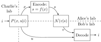
Figure 1: Zero-error source-channel coding.

There are a number of reasons one might wish to consider such a scenario. For instance, suppose that $x=i$ always. The side information $u$ might have originated from a previous noisy transmission of $x$ from Alice to Bob. The goal is to resend using channel $\mathcal{N}$ in order to fill in the missing information. Or, the communication complexity of bipartite function evaluation fits into this model. Suppose that Alice and Bob receive $x$ and $u$, respectively, from a referee Charlie. Alice must send a message to Bob such that Bob may evaluate some function $g(x,u)$. To fit this into the model of Fig. 1, imagine that Charlie first chooses a value $i$ for $g$, then sends Alice and Bob some $x,u$ pair such that $g(x,u)=i$. From the perspective of Alice and Bob, determining $i$ is equivalent to evaluating $g(x,u)$. One may ask how many bits Alice needs to send to Bob to accomplish this.

In general, Alice’s strategy is to encode her input $x$ using some function $f:X\to S$ before sending it through the channel (a randomized strategy never helps when zero-error is required). As before, Bob receives a value $v$ with probability $\mathcal{N}(v|s)$. The values $u$ and $v$ must be sufficient for Bob to compute $i$. For a given $u$, Bob knows Alice’s input comes from the set $\{x:\exists i\textrm{ such that }P(x,u|i)\neq 0\}$. Bob only needs to distinguish between the values of $x$ corresponding to different $i$, since his goal is to determine $i$. Define a graph $G$ with vertices $V(G)=X$ and with edges between Alice inputs that Bob sometimes needs to distinguish:

$$x\sim_{G}y\iff\exists u,\exists i\neq j\textrm{ s.t. }P(x,u|i)P(y,u|j)\neq 0.$$ (2)

This is the characteristic graph of the source $P$. If Bob must sometimes distinguish $x$ from $y$ then Alice’s encoding must ensure that $x$ and $y$ never get mapped to the same output by the noisy channel. In other words, her encoding must satisfy $f(x)\sim_{H}f(y)$ whenever $x\sim_{G}y$. By definition, this is possible precisely when $G$ is homomorphic to $H$.

Definition 1.

Let $G$ and $H$ be graphs without loops. $G$ is homomorphic to $H$, written $G\to H$, if there is a function $f:V(G)\to V(H)$ such that $x\sim y\implies f(x)\sim f(y)$. The function $f$ is said to be a homomorphism from $G$ to $H$.

Graph homomorphisms are examined in great detail in [18, 19]. We state here some basic facts that can be immediately verified.

Proposition 2.

Let $F,G,H$ be graphs without loops.

1. If $F\to G$ and $G\to H$ then $F\to H$.

2. If $G$ is a subgraph of $H$ then $G\to H$.

3. The clique number $\omega(H)$ is the largest $n$ such that $K_{n}\to H$.

4. The chromatic number $\chi(G)$ is the smallest $n$ such that $G\to K_{n}$.

The above arguments can be summarized as follows.

Proposition 3.

There exists a zero-error source-channel coding protocol for source $P(x,u|i)$ and channel $\mathcal{N}(v|s)$ if and only if $G\to H$ where $G$ is the characteristic graph of the source, (2), and $H$ is the distinguishability graph of the channel, (1).

As required by Definition 1, neither $G$ nor $H$ have loops. More precisely, $G$ has a loop if and only if there is an $x,u$ that can occur for two different inputs by Charlie. In this case it is impossible for Alice and Bob to recover Charlie’s input, no matter how much communication is allowed.

We emphasize that, although we refer to source-channel coding and use the associated terminology, we are actually considering something a bit more general since we use a source $P(x,u|i)$, with Bob answering $i$, rather than a source $P(x,u)$, with Bob answering $x$. Standard source-channel coding, which can be recovered by setting $P(x,u|i)\neq 0\iff x=i$, was characterized in terms of graph homomorphisms in [10]. Our generalization does not substantially change the theory, and will allow a smoother transition to the quantum version (in the next section).

The Lovász number of the complementary graph, $\overline{\vartheta}(G)=\vartheta({\overline{G}})$, is given by the following dual (and equivalent) semidefinite programs: [20, 21]

$$\overline{\vartheta}(G) =\max\{\left\lVert I+T\right\rVert:I+T\succeq 0,$$

$$\hphantom{=\max\{\;}T_{ij}=0\textnormal{ for }i\not\sim j\},$$ (3)

$$\overline{\vartheta}(G) =\min\{\lambda:\exists Z\succeq J,Z_{ii}=\lambda,$$

$$\hphantom{=\max\{\;}Z_{ij}=0\textnormal{ for }i\sim j\},$$ (4)

where we assume that $G$ has no loops. The norm here is the operator norm (equal to the largest singular value), $J$ is the matrix with every entry equal to 1, and $Z\succeq J$ means that $Z-J$ is positive semidefinite. This quantity is a homomorphism monotone in the sense that [14]

$$G\to H\implies\overline{\vartheta}(G)\leq\overline{\vartheta}(H).$$ (5)

Consequently (see Proposition 2) we have the Lovász sandwich theorem

$$\omega(G)\leq\overline{\vartheta}(G)\leq\chi(G).$$ (6)

Since source-channel coding is only possible when $G\to H$, it follows that $\overline{\vartheta}(G)\leq\overline{\vartheta}(H)$ is a necessary condition. Two related quantities, Schrijver’s $\overline{\vartheta}^{\prime}$ and Szegedy’s $\overline{\vartheta}^{+}$, which will be defined in Section VII, have similar monotonicity properties [14] so they provide similar bounds.

Proposition 4.

One-shot source-channel coding is possible only if $\overline{\vartheta}(G)\leq\overline{\vartheta}(H)$, $\overline{\vartheta}^{\prime}(G)\leq\overline{\vartheta}^{\prime}(H)$, and $\overline{\vartheta}^{+}(G)\leq\overline{\vartheta}^{+}(H)$, where $G$ is the characteristic graph of the source, (2), and $H$ is the distinguishability graph of the channel, (1).

Traditionally, source-channel coding has been studied in the case where $P(x,u|i)\neq 0$ only when $x=i$. In this case, the following bound holds [10]:

Proposition 5.

Suppose $P(x,u|i)\neq 0$ only when $x=i$ and let graphs $G$ and $H$ be given by (2) and (1). Then $m$ parallel instances of the source can be sent using $n$ parallel instances of the channel only if

$$\frac{n}{m}\geq\frac{\log\overline{\vartheta}(G)}{\log\overline{\vartheta}(H)}.$$

We will always take logarithms to be base 2. The infimum of $n/m$ (equivalent to the limit as $m\to\infty$) is known as the cost rate; Proposition 5 can be interpreted as an upper bound on the cost rate. This bound relies on the fact that $\overline{\vartheta}$ is multiplicative under various graph products, a property not shared by $\overline{\vartheta}^{\prime}$ or $\overline{\vartheta}^{+}$. Propositions 4 and 5 apply also to the case of entanglement assisted source-channel coding, still with classical inputs and a classical channel [12]. We will later show (Proposition 21) that the condition $P(x,u|i)\neq 0$ only when $x=i$ is not necessary in Proposition 5.

With some interesting caveats, these two theorems in fact also apply to a generalization of source-channel coding in which the source produces bipartite entangled states and in which the channel is quantum. The rest of this paper is devoted to development of this theory.

III Non-commutative graph theory

Given a graph $G$ on vertices $V(G)=\{1,\dots,n\}$ we may define the operator space

$$S =\textnormal{span}\{\left|{x}\right\rangle\left\langle{y}\right|:x\sim y\}\subseteq\mathcal{L}(\mathbb{C}^{n})$$ (7)

where $\left|{x}\right\rangle$ and $\left|{y}\right\rangle$ are basis vectors from the standard basis. Because we consider symmetric rather than directed graphs, this space is Hermitian: $A\in S\iff A^{\dagger}\in S$ (more succinctly, $S=S^{\dagger}$). If $G$ has no loops, $S$ is trace-free (it consists only of trace-free operators). If $G$ has loops on all vertices, $S$ contains the identity.

Concepts from graph theory can be rephrased in terms of such operator spaces. For example, for trace-free spaces the clique number can be defined as the size of the largest set of nonzero vectors $\{\left|{\psi_{i}}\right\rangle\}$ such that $\left|{\psi_{i}}\right\rangle\left\langle{\psi_{j}}\right|\in S$ for all $i\neq j$. Note that since $S$ is trace-free, these vectors must be orthogonal. Although not immediately obvious, this is indeed equivalent to $\omega(G)$ when $S$ is defined as in (7).

Having defined clique number in terms of operator spaces, one can drop the requirement that $S$ be of the form (7) and can speak of the clique number of an arbitrary Hermitian subspace. Such subspaces, thought of in this way, are called non-commutative graphs [1]. Note that [1] requires $S$ to contain the identity, but we drop this requirement and insist only that $S=S^{\dagger}$. Such a generalization is analogous to allowing the vertices of a graph to not have loops. Dropping also the condition $S=S^{\dagger}$ would give structures analogous to directed graphs, however we will not have occasion to consider this.

To draw clear distinction between non-commutative graphs and the traditional kind, we will often refer to the latter as classical graphs. We will say $S$ derives from a classical graph if $S$ is of the form (7).

The distinguishability graph of a quantum channel $\mathcal{N}:\mathcal{L}(A)\to\mathcal{L}(B)$ with Kraus operators $\{N_{i}\}$ can be defined as

$$T =(\textnormal{span}\{N_{i}^{\dagger}N_{j}:\forall i,j\})^{\perp}\subseteq\mathcal{L}(A)$$ (8)

where $\perp$ denotes the perpendicular subspace under the Hilbert–Schmidt inner product $\left<X,Y\right>=\textnormal{Tr}(X^{\dagger}Y)$. For a classical channel this is equal to (7) with $G$ given by (1). The space $\textnormal{span}\{N_{i}^{\dagger}N_{j}\}$ (the confusability graph) was considered in [4, 2, 3, 1]; however, we consider the perpendicular space for the same reason that we considered the distinguishability rather than the confusability graph in Section II: it leads to simpler notation especially when discussing homomorphisms. It will be convenient to use the notation

$$N:=\textnormal{span}\{N_{i}\},$$

and likewise for other sets of Kraus operators so that (8) becomes simply

$$T=(N^{\dagger}N)^{\perp},$$ (9)

with the multiplication of two operator spaces defined to be the linear span of the products of operators from the two spaces. Note that the closure condition for Kraus operators gives $\sum_{i}N_{i}^{\dagger}N_{i}=I\implies I\in N^{\dagger}N\implies I\perp T$. Therefore $T$ is trace-free.

In [1] a generalization of the Lovász $\vartheta(G)$ number was provided for non-commutative graphs, which they called $\tilde{\vartheta}(S)$. We present the definition in terms of $\overline{\vartheta}(S):=\tilde{\vartheta}(S^{\perp})$, which should be thought of as a generalization of $\overline{\vartheta}(G)=\vartheta({\overline{G}})$.

Definition 6 ([1]).

Let $S\subseteq\mathcal{L}(A)$ be a trace-free non-commutative graph. Let $A^{\prime}$ be an ancillary system of the same dimension as $A$, and define the vector $\left|{\Phi}\right\rangle=\sum_{i}\left|{i}\right\rangle_{A}\otimes\left|{i}\right\rangle_{A^{\prime}}$. Then $\overline{\vartheta}(S)$ is defined by the following dual (and equivalent) programs:

$$\overline{\vartheta}(S) =\max\{\left\lVert I+X\right\rVert:X\in S\otimes\mathcal{L}(A^{\prime}),I+X\succeq 0\},$$ (10)

$$\overline{\vartheta}(S) =\min\{\left\lVert\textnormal{Tr}_{A}Y\right\rVert:Y\in S^{\perp}\otimes\mathcal{L}(A^{\prime}),Y\succeq\left|{\Phi}\right\rangle\left\langle{\Phi}\right|\}.$$ (11)

We will use the notation $\tilde{\vartheta}(S^{\perp})=\overline{\vartheta}(S)$.

When $S$ derives from loop-free graph $G$ via (7), this reduces to the standard Lovász number: $\overline{\vartheta}(S)=\overline{\vartheta}(G)$. Similarly, when $S$ derives from a graph $G$ having loops on all vertices, $\tilde{\vartheta}(S)=\vartheta(G)$. Analogous to the classical case, $\overline{\vartheta}(S)$ gives an upper bound on the zero-error capacity of a quantum channel. In fact, it even gives an upper bound on the zero-error entanglement assisted capacity [1].

Independence number for non-commutative graphs has been investigated in [4, 2, 3, 1], and in [1] the authors posed the question of whether further concepts from graph theory can be generalized as well. We carry out this program by generalizing graph homomorphisms, which will in turn lead to a chromatic number for non-commutative graphs. These generalized graph homomorphisms will characterize quantum source-channel coding in analogy to Proposition 3. In fact, one could define non-commutative graph homomorphisms as being the relation that gives a generalization of Proposition 3, but we choose instead to provide more direct justification for our definition.

We begin by describing ordinary graph homomorphisms in terms of operator spaces of the form (7); this will lead to a natural generalization to non-commutative graphs. Suppose that $S\subseteq\mathcal{L}(A)$ and $T\subseteq\mathcal{L}(B)$ are derived from graphs $G$ and $H$ via (7), and consider a function $f:V(G)\to V(H)$. In terms of $S$ and $T$, the homomorphism condition $x\sim_{G}y\implies f(x)\sim_{H}f(y)$ becomes

$$\left|{x}\right\rangle\left\langle{y}\right|\in S\implies\left|{f(x)}\right\rangle\left\langle{f(y)}\right|\in T,$$ (12)

where $\left|{x}\right\rangle$ and $\left|{y}\right\rangle$ are vectors from the standard basis. Consider the classical channel that maps $x\to f(x)$. Viewed as a quantum channel, this can be written as the superoperator $\mathcal{E}:\mathcal{L}(A)\to\mathcal{L}(B)$ with the action $\mathcal{E}(\left|{x}\right\rangle\left\langle{x}\right|)=\left|{f(x)}\right\rangle\left\langle{f(x)}\right|$. The Kraus operators of this channel are $E_{x}=\left|{f(x)}\right\rangle\left\langle{x}\right|$. Again using the notation $E=\textnormal{span}\{E_{i}\}$, (12) can be written $ESE^{\dagger}\subseteq T$. The generalization to non-commutative graphs is obtained by dropping the condition that $\mathcal{E}$ be a classical channel, allowing instead arbitrary completely positive trace preserving (CPTP) maps.

Definition 7.

Let $S\subseteq\mathcal{L}(A)$ and $T\subseteq\mathcal{L}(B)$ be trace-free non-commutative graphs. We write $S\to T$ if there exists a completely positive trace preserving (CPTP) map $\mathcal{E}:\mathcal{L}(A)\to\mathcal{L}(B)$ with Kraus operators $\{E_{i}\}$ such that

$$ESE^{\dagger} \subseteq T\textrm{ or, equivalently,}$$ (13)

$$E^{\dagger}T^{\perp}E \subseteq S^{\perp}.$$ (14)

Equivalently, $S\to T$ if and only if there is a Hilbert space $C$ and an isometry $J:A\to B\otimes C$ such that

$$JSJ^{\dagger}\subseteq T\otimes\mathcal{L}(C)\textrm{ or, equivalently,}$$ (15)

$$J^{\dagger}(T^{\perp}\otimes\mathcal{L}(C))J\subseteq S^{\perp}.$$ (16)

We will say that the subspace $E$, or the Kraus operators $\{E_{i}\}$, or the isometry $J$, is a homomorphism from $S$ to $T$.

That (13)-(16) are equivalent can be seen as follows. $\eqref{eq:homq_def1}\iff(\textnormal{Tr}\{ese^{\prime{\dagger}}t^{\prime}\}=0\;\forall e,e^{\prime}\in E,s\in S,t^{\prime}\in T^{\perp})\iff\eqref{eq:homq_def2}$. Similar reasoning shows $\eqref{eq:homq_def3}\iff\eqref{eq:homq_def4}$, using $(T\otimes\mathcal{L}(C))^{\perp}=T^{\perp}\otimes\mathcal{L}(C)$. Equivalence of (14) and (16) follows from the fact that $E=\textnormal{span}_{\left|{\phi}\right\rangle}\{(I\otimes\left\langle{\phi}\right|)J\}$ where $J$ is related to $\mathcal{E}$ by Stinespring’s dilation theorem.

When $S$ and $T$ derive from classical graphs Definition 7 is equivalent to Definition 1, as we will now show.

Theorem 8.

For non-commutative graphs that derive from classical graphs, Definitions 1 and 7 coincide. In other words, if $S$ and $T$ derive from graphs $G$ and $H$ according to the recipe (7) then $G\to H\iff S\to T$.

Proof.

Let $S$ and $T$ be non-commutative graphs deriving from classical graphs $G$ and $H$.

($\implies$) Suppose $G\to H$. By Definition 1 there is an $f:G\to H$ such that $x\sim_{G}y\implies f(x)\sim_{H}f(y)$. Consider the set of Kraus operators $E_{x}=\left|{f(x)}\right\rangle\left\langle{x}\right|$. Then,

$$ESE^{\dagger} =\textnormal{span}\{E_{i}\left|{x}\right\rangle\left\langle{y}\right|E_{j}^{\dagger}:i,j,x\sim_{G}y\}$$

$$=\textnormal{span}\{\left|{f(x)}\right\rangle\left\langle{f(y)}\right|:x\sim_{G}y\}$$

$$\subseteq T.$$

($\impliedby$) Suppose $S\to T$. By Definition 7 there is a channel $\mathcal{E}:\mathcal{L}(A)\to\mathcal{L}(B)$ such that $ESE^{\dagger}\subseteq T$. For each vertex $x$ of $G$, there is an $i(x)$ such that $E_{i(x)}\left|{x}\right\rangle$ does not vanish. Pick an arbitrary nonvanishing index of the vector $E_{i(x)}\left|{x}\right\rangle$ and call this $f(x)$ so that $\left\langle{f(x)}\right|E_{i(x)}\left|{x}\right\rangle\neq 0$.

Now consider any edge $x\sim_{G}y$. We have

$$\left|{x}\right\rangle\left\langle{y}\right|\in S \implies E\left|{x}\right\rangle\left\langle{y}\right|E^{\dagger}\in T$$

$$\implies E_{i(x)}\left|{x}\right\rangle\left\langle{y}\right|E^{\dagger}_{i(y)}\in T.$$

Define $\tau:=E_{i(x)}\left|{x}\right\rangle\left\langle{y}\right|E^{\dagger}_{i(y)}$. Then $\tau\in T$ and

$$\left\langle{f(x)}\middle|{\tau}\middle|{f(y)}\right\rangle\neq 0 \implies\textnormal{Tr}\{\tau\left|{f(y)}\right\rangle\left\langle{f(x)}\right|\}\neq 0$$

$$\implies\left|{f(x)}\right\rangle\left\langle{f(y)}\right|\not\in T^{\perp}$$

$$\implies\left|{f(x)}\right\rangle\left\langle{f(y)}\right|\in T$$

$$\implies f(x)\sim_{H}f(y).$$

Therefore $x\sim_{G}y\implies f(x)\sim_{H}f(y)$. ∎

Definition 7 could be loosened to require only that $\sum_{i}E_{i}^{\dagger}E_{i}$ be invertible (equivalently $E\left|{\psi}\right\rangle\neq\{0\}$ for all $\left|{\psi}\right\rangle$, equivalently $J^{\dagger}J$ invertible) rather than $\mathcal{E}$ being trace preserving. Theorem 8 would still hold; however, Definition 7 as currently stated has an operational interpretation in terms of quantum source-channel coding (which we will introduce in Section IV) and satisfies the monotonicity relation $S\to T\implies\overline{\vartheta}(S)\leq\overline{\vartheta}(T)$ (which we will show in Section V). Hilbert space structure seems to be important for non-commutative graphs, so it is reasonable to require that $J$ preserve this structure (i.e. $J$ should be an isometry).

As a guide to the intuition, one should not think of $ESE^{\dagger}$ in (13) as density operators $\rho\in S$ going into a channel, like $\sum_{i}E_{i}\rho E_{i}^{\dagger}$, but rather as a mechanism for comparing the action of the channel on two different states, something like $\{E_{i}\left|{\psi}\right\rangle\left\langle{\phi}\right|E_{j}^{\dagger}:\forall i,j\}$ with $\left|{\psi}\right\rangle\left\langle{\phi}\right|\in S$. But this is only a rough intuition, as $S$ might not necessary be composed of dyads $\left|{\psi}\right\rangle\left\langle{\phi}\right|$. The two copies of $E$ here are analogous to the two Kraus operators appearing in the Knill–Laflamme condition, which we will explore in Section IV. Note that $E\left|{\psi}\right\rangle$ is equal to the support of $\mathcal{E}(\left|{\psi}\right\rangle\left\langle{\psi}\right|)$.

The non-commutative graph homomorphism of Definition 7 satisfies properties analogous to those of Proposition 2.

Proposition 9.

Let $R,S,T$ be trace-free non-commutative graphs.

1. If $R\to S$ and $S\to T$ then $R\to T$.

2. If $S\subseteq T$ then $S\to T$. More generally, if $J$ is an isometry and $JSJ^{\dagger}\subseteq T$ then $S\to T$.

Proof.

Item 1 follows from considering the composition of channels associated with the homomorphisms $R\to S$ and $S\to T$. Item 2 follows trivially from (15), taking space $C$ to be trivial (one dimensional). ∎

(The condition that appears above, $JSJ^{\dagger}\subseteq T$ with $J$ an isometry, seems to be a reasonable generalization of the notion of subgraphs for non-commutative graphs, although we won’t be making use of this concept. Note that [1] defined induced subgraphs as $J^{\dagger}SJ$. It appears that these two definitions are somewhat incompatible.)

For classical graphs the clique number is the greatest $n$ such that $K_{n}\to G$ and the chromatic number is the least $n$ such that $G\to K_{n}$. We use this to extend these concepts to non-commutative graphs. In the previous section, the complete graph $K_{n}$ was defined to have no loops. The corresponding non-commutative graph, defined via (7), is $\textnormal{span}\{\left|{x}\right\rangle\left\langle{y}\right|:x\neq y\}$, the space of matrices with zeros on the diagonal. However, it is reasonable to also consider $(\mathbb{C}I)^{\perp}$, the space of trace-free operators. We consider both.

Definition 10.

For $n\geq 1$ define the classical and quantum complete graphs

$$K_{n} =\textnormal{span}\{\left|{x}\right\rangle\left\langle{y}\right|:x\neq y\}\subseteq\mathcal{L}(\mathbb{C}^{n}),$$

$$Q_{n} =(\mathbb{C}I)^{\perp}\subseteq\mathcal{L}(\mathbb{C}^{n}).$$

One can think of $K_{n}$ as consisting of the operators orthogonal to the “classical loops” ${\left|{x}\right\rangle\left\langle{x}\right|}$ and $Q_{n}$ as consisting of the operators orthogonal to the “coherent loop” $I$. We use these to define clique, independence, and chromatic numbers for non-commutative graphs. In Section IV we will see that all of these quantities have operational interpretations in the context of communication problems. These quantities, and others, are summarized in Section IV.

Definition 11.

Let $S$ be a trace-free non-commutative graph. We define the following quantities.

1. $\omega(S)$ is the greatest $n$ such that $K_{n}\to S$

2. $\omega_{q}(S)$ is the greatest $n$ such that $Q_{n}\to S$

3. $\alpha(S^{\perp})=\omega(S)$ and $\alpha_{q}(S^{\perp})=\omega_{q}(S)$. Note that $I\in S^{\perp}$.

4. $\chi(S)$ is the least $n$ such that $S\to K_{n}$, or $\infty$ if $S\not\to K_{n}$ for all $n$

5. $\chi_{q}(S)$ is the least $n$ such that $S\to Q_{n}$

The quantities $\omega_{q}$ and $\chi_{q}$ are not to be confused with the quantities of similar name that are discussed in the context of Bell-like nonlocal games [15, 16, 17].

When $S$ derives from a classical graph $G$, our $\omega$ and $\chi$ correspond to the ordinary definitions of clique number and chromatic number and our $\chi_{q}$ corresponds to the orthogonal rank $\xi(G)$. This will be proved shortly. For non-commutative graphs with $I\in S$, our definition of $\alpha(S)$ and $\alpha_{q}(S)$ corresponds to that of [1, 2, 3, 4], as we will show in Theorem 13. In other words, when $S=N^{\dagger}N$ is the confusability graph of a channel $\mathcal{N}$, $\alpha(S)$ and $\alpha_{q}(S)$ correspond to the one-shot classical and quantum capacities; when $S=(N^{\dagger}N)^{\perp}$ the same can be said for $\omega(S)$ and $\omega_{q}(S)$.

Theorem 12.

Let $S$ be the non-commutative graph associated with a classical loop-free graph $G$. Then $\omega(S)=\omega(G)$, $\chi(S)=\chi(G)$, $\chi_{q}(S)=\xi(G)$, and $\omega_{q}(S)=1$.

Proof.

$\omega(S)=\omega(G)$ and $\chi(S)=\chi(G)$ follow directly from Definition 11 and Propositions 2 and 8.

An orthogonal representation of $G$ is a map from vertices to nonzero vectors such that adjacent vertices correspond to orthogonal vectors. The orthogonal rank $\xi(G)$ is defined to be the smallest possible dimension of an orthogonal representation. Let $\{\left|{\psi_{x}}\right\rangle\}_{x\in V(G)}\subseteq\mathcal{L}(\mathcal{C}^{n})$ be an orthogonal representation of $G$. Without loss of generality assume these vectors to be normalized. The Kraus operators $E_{x}=\left|{\psi_{x}}\right\rangle\left\langle{i}\right|$ provide a homomorphism $S\to Q_{n}$. So $\chi_{q}(S)\leq\xi(G)$.

Conversely, suppose a set of Kraus operators $\{E_{i}\}$ provides a homomorphism $S\to Q_{n}$ with $n=\chi_{q}(S)$. Because $\sum_{i}E_{i}^{\dagger}E_{i}=I$, for each $x\in G$ there is an $i(x)$ such that $E_{i(x)}\left|{x}\right\rangle$ does not vanish. Define $\left|{\psi_{x}}\right\rangle=E_{i(x)}\left|{x}\right\rangle$. For any edge $x\sim y$ of $G$ we have

$$\left|{x}\right\rangle\left\langle{y}\right|\in S \implies E\left|{x}\right\rangle\left\langle{y}\right|E^{\dagger}\in Q_{n}$$

$$\implies\left|{\psi_{x}}\right\rangle\left\langle{\psi_{y}}\right|\in Q_{n}$$

$$\implies\left\langle{\psi_{x}}\middle|{\psi_{y}}\right\rangle=0.$$

So $\{\left|{\psi_{x}}\right\rangle\}_{x\in V(G)}$ is an orthogonal representation of $G$ of dimension $n$, giving $\xi(G)\leq\chi_{q}(S)$.

$\omega_{q}(S)=1$ because it is not possible to have $Q_{n}\to S$ if $n>1$. For, suppose that such a homomorphism $E$ existed. There must be some $x\in V(G)$ and some $i$ such that $\left\langle{x}\right|E_{i}\neq 0$. Since $G$ is loop free, ${\left|{x}\right\rangle\left\langle{x}\right|}\in S^{\perp}$ so $E_{i}^{\dagger}{\left|{x}\right\rangle\left\langle{x}\right|}E_{i}\in E^{\dagger}S^{\perp}E$. But $Q_{n}^{\perp}=\mathbb{C}I$ contains no rank-1 operators so $E^{\dagger}S^{\perp}E\not\subseteq Q_{n}^{\perp}$ and $E$ cannot be a homomorphism from $Q_{n}$ to $S$. ∎

Theorem 13.

Let $S\subseteq\mathcal{L}(A)$ be a non-commutative graph with $I\in S$. Then our $\alpha(S)$ and $\alpha_{q}(S)$ are equivalent to the independence number and quantum independence number of [1, 2, 3, 4].

Proof.

This is a consequence of the operational interpretation of non-commutative graph homomorphisms which we will prove in Section IV; however, we give here a direct proof. The independence number of [1] is the largest number of nonzero vectors $\{\left|{\psi_{i}}\right\rangle\}_{i}$ such that

$$\left|{\psi_{i}}\right\rangle\left\langle{\psi_{j}}\right|\in S^{\perp}\textrm{ when }i\neq j.$$ (17)

Given such a collection of $n$ vectors one can define $E_{i}:\mathbb{C}^{n}\to A$ as $E_{i}=\left|{\psi_{i}}\right\rangle\left\langle{i}\right|$. Since $I\in S$, (17) requires orthogonal vectors; thus $\sum_{i}E_{i}^{\dagger}E_{i}=I$ so these $\{E_{i}\}$ are indeed Kraus operators. Now,

$$EK_{n}E^{\dagger} =\textnormal{span}\{E_{i^{\prime}}\left|{i}\right\rangle\left\langle{j}\right|E_{j^{\prime}}:i\neq j\}$$

$$=\textnormal{span}\{\left|{\psi_{i}}\right\rangle\left\langle{\psi_{j}}\right|:i\neq j\}\subseteq S^{\perp},$$

giving $K_{n}\to S^{\perp}$, or $\alpha(S)\geq n$.

Conversely, take $n=\alpha(S)$. By the definition of $\alpha(S)$, we have $K_{n}\to S^{\perp}$. Let $\{E_{i}\}$ be the Kraus operators that satisfy $EK_{n}E^{\dagger}\subseteq S^{\perp}$, as per Definition 7. Since $\sum_{k}E_{k}^{\dagger}E_{k}=I$, for each $i\in\{1,\dots,n\}$ there must be some $k(i)$ such that $E_{k(i)}\left|{i}\right\rangle\neq 0$. Define $\left|{\psi_{i}}\right\rangle=E_{k(i)}\left|{i}\right\rangle$. Then for $i\neq j$, $EK_{n}E^{\dagger}\subseteq S^{\perp}\implies\left|{\psi_{i}}\right\rangle\left\langle{\psi_{j}}\right|\in S^{\perp}$.

The quantum independence number is the largest rank projector $P$ such that $PSP=\mathbb{C}P$. Suppose we have such a projector. Let $n=\textnormal{rank}(P)$ and let $J:\mathbb{C}^{n}\to A$ be an isometry such that $JJ^{\dagger}=P$. Then $J^{\dagger}SJ=J^{\dagger}PSPJ=\mathbb{C}J^{\dagger}PJ=\mathbb{C}I=Q_{n}^{\perp}$. By (16), taking $C$ to be the trivial (one-dimensional) space, this gives $Q_{n}\to S^{\perp}$, or $\alpha_{q}(S)\geq n$.

Conversely, take $n=\alpha_{q}(S)$. Since $Q_{n}\to S^{\perp}$, there are Kraus operators $\{E_{i}\}$ such that $E^{\dagger}SE\subseteq Q_{n}^{\perp}=\mathbb{C}I$, as per (14). At least one of these Kraus operators, call it $E_{0}$, must satisfy $E_{0}^{\dagger}E_{0}\neq 0$. Since $I\in S$, $E_{0}^{\dagger}IE_{0}\in E^{\dagger}SE\subseteq\mathbb{C}I$, so $E_{0}^{\dagger}E_{0}=\alpha I$ with $\alpha\neq 0$. Then $J:=E_{0}/\sqrt{\alpha}$ is an isometry and $P:=JJ^{\dagger}$ is a rank $n$ projector. Furthermore, $PSP=JE_{0}^{\dagger}SE_{0}J^{\dagger}\subseteq\mathbb{C}JIJ^{\dagger}=\mathbb{C}P$. ∎

IV Quantum source-channel coding

We construct a quantum version of source-channel coding, as depicted in Fig. 2. The channel $\mathcal{N}$ from Alice to Bob is now a quantum channel. Instead of classical inputs $x$ and $u$, Alice and Bob receive a bipartite quantum state. One may imagine that a referee Charlie chooses a bipartite mixed state $\rho_{i}\in\mathcal{L}(A)\otimes\mathcal{L}(B)$ from some finite collection and sends the $A$ subsystem to Alice and the $B$ subsystem to Bob. The details of the collection $\{\rho_{i}\}$ are known ahead of time to Alice and Bob. Bob must determine $i$, with zero chance of error, using Alice’s message and his share of $\rho_{i}$. We call this discrete quantum source-channel coding (discrete QSCC). Here “discrete” refers to $i$; we will later quantize even this. Discrete QSCC reduces to classical source-channel coding (Section II) by taking $\mathcal{N}$ to be a classical channel and the source to be of the form $\rho_{i}=\sum_{xu}P(x,u|i){\left|{x}\right\rangle\left\langle{x}\right|}\otimes{\left|{u}\right\rangle\left\langle{u}\right|}$.

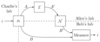
Figure 2: Discrete quantum source-channel coding (discrete QSCC).

The most general strategy is for Alice to encode her portion of $\rho_{i}$ using some quantum operation (some CPTP map) $\mathcal{E}:\mathcal{L}(A)\to\mathcal{L}(A^{\prime})$ before sending it through $\mathcal{N}$ to Bob, and for Bob to perform a POVM measurement on the joint state consisting of his portion of $\rho_{i}$ and the message received from Alice. After receiving Alice’s message, Bob is in possession of the mixed state

$$\sigma_{i} =\mathcal{N}(\mathcal{E}(\rho_{i}))$$

$$=\sum_{jk}(N_{k}E_{j}\otimes I)\rho_{i}(E_{j}^{\dagger}N_{k}^{\dagger}\otimes I)$$

$$=\sum_{jkl}(N_{k}E_{j}\otimes I)\left|{\psi_{il}}\right\rangle\left\langle{\psi_{il}}\right|(E_{j}^{\dagger}N_{k}^{\dagger}\otimes I),$$ (18)

where the unnormalized vectors $\left|{\psi_{il}}\right\rangle$ are defined according to $\rho_{i}=\sum_{l}\left|{\psi_{il}}\right\rangle\left\langle{\psi_{il}}\right|$. There is a measurement that can produce the value $i$ with zero error if and only if the states $\sigma_{i}$ and $\sigma_{i^{\prime}}$ are orthogonal whenever $i\neq i^{\prime}$. Since each term of (18) is positive semidefinite we have, with $\left<\cdot,\cdot\right>$ denoting the Hilbert–Schmidt inner product,

$$\left<\sigma_{i},\sigma_{i^{\prime}}\right>=0 \iff\left\langle{\psi_{il}}\middle|{(E_{j}^{\dagger}N_{k}^{\dagger}\otimes I)(N_{k^{\prime}}E_{j^{\prime}}\otimes I)}\middle|{\psi_{i^{\prime}l^{\prime}}}\right\rangle=0$$

$$\hskip 100.00015pt\forall j,j^{\prime},k,k^{\prime},l,l^{\prime}$$

$$\iff\left<E_{j^{\prime}}\textnormal{Tr}_{B}\{\left|{\psi_{i^{\prime}l^{\prime}}}\right\rangle\left\langle{\psi_{il}}\right|\}E_{j}^{\dagger},N_{k^{\prime}}^{\dagger}N_{k}\right>=0$$

$$\hskip 100.00015pt\forall j,j^{\prime},k,k^{\prime},l,l^{\prime}$$

$$\iff E\cdot\textnormal{Tr}_{B}\{\left|{\psi_{i^{\prime}l^{\prime}}}\right\rangle\left\langle{\psi_{il}}\right|\}\cdot E^{\dagger}\perp N^{\dagger}N$$

$$\hskip 100.00015pt\forall l,l^{\prime}.$$

By Definition 7, such an encoding $\mathcal{E}$ exists if and only if $\textnormal{span}\{\textnormal{Tr}_{B}\{\left|{\psi_{i^{\prime}l^{\prime}}}\right\rangle\left\langle{\psi_{il}}\right|\}:\forall i\neq i^{\prime},\forall l,l^{\prime}\}\to(N^{\dagger}N)^{\perp}$. This immediately leads to the following theorem.

Theorem 14.

Consider discrete QSCC (Fig. 2) with $i\in\{1,\dots,n\}$. For each $i$, let $\left|{\psi_{i}}\right\rangle\in A\otimes B\otimes C$ be a purification of $\rho_{i}\in\mathcal{L}(A)\otimes\mathcal{L}(B)$. Define the isometry $J:R\to A\otimes B\otimes C$ with $R=\mathbb{C}^{n}$ as $J=\sum_{i=1}^{n}\left|{\psi_{i}}\right\rangle\left\langle{i}\right|$. There is a zero-error strategy if and only if $S\to T$ where $T$ is the distinguishability graph of $\mathcal{N}$, given by (9), and $S$ is the characteristic graph of the source, given by

$$S=\textnormal{Tr}_{BC}\{\mathcal{L}(C)JK_{n}J^{\dagger}\}.$$ (19)

Suppose that Alice and Bob also share an entanglement resource $\left|{\lambda}\right\rangle\in A^{\prime\prime}\otimes B^{\prime\prime}$. This can be absorbed into the source, considering the source to be $\rho_{i}\otimes{\left|{\lambda}\right\rangle\left\langle{\lambda}\right|}$. Then (19) becomes $\textnormal{Tr}_{BC}\{\mathcal{L}(C)JK_{n}J^{\dagger}\}\otimes\Lambda$ where $\Lambda=\textnormal{Tr}_{B^{\prime\prime}}\{{\left|{\lambda}\right\rangle\left\langle{\lambda}\right|}\}$. This motivates the following definition:

Definition 15.

Let $S$ and $T$ be trace-free non-commutative graphs. We say there is an entanglement assisted homomorphism $S\stackrel{{\scriptstyle*}}{{\to}}T$ if there exists an operator $\Lambda\succ 0$ such that $S\otimes\Lambda\to T$. The entanglement assisted quantities $\alpha_{*}(S)$, $\alpha_{q*}(S)$, $\omega_{*}(S)$, $\omega_{q*}(S)$, $\chi_{*}(S)$, and $\chi_{q*}(S)$ are defined by using $\stackrel{{\scriptstyle*}}{{\to}}$ rather than $\to$ in Definition 11.

If $S$ and $T$ are induced by classical graphs $G$ and $H$ then $S\stackrel{{\scriptstyle*}}{{\to}}T$ if and only if $G\stackrel{{\scriptstyle*}}{{\to}}H$ as defined in [11, 12]. This equivalence follows from the fact that $S\stackrel{{\scriptstyle*}}{{\to}}T$ and $G\stackrel{{\scriptstyle*}}{{\to}}H$ have identical operational interpretation in terms of entanglement assisted source-channel coding. Our $\alpha_{*}(S)$ corresponds to the entanglement assisted independence number of [1] and if $S$ derives from a classical graph our $\chi_{*}(S)$ corresponds to the entangled chromatic number of [11, 12]. These quantities, and others, are summarized in Section IV.

We give some examples.

• Dense coding. Let $\rho_{i}={\left|{i}\right\rangle\left\langle{i}\right|}_{A_{1}}\otimes{\left|{\lambda}\right\rangle\left\langle{\lambda}\right|}_{A_{2}B}$ where $i\in\{1,\dots,m\}$ represents the codeword to be transmitted and ${\left|{\lambda}\right\rangle\left\langle{\lambda}\right|}_{A_{2}B}$ is an entanglement resource shared by Alice and Bob. Take $\mathcal{N}$ to be a noiseless quantum channel of dimension $n$ (i.e. a channel of $\log n$ qubits). By Theorem 14, dense coding is possible if and only if $K_{m}\otimes\textnormal{Tr}_{B}\{{\left|{\lambda}\right\rangle\left\langle{\lambda}\right|}\}\to Q_{n}$. The well known bound $m\leq n^{2}$ for dense coding gives $(K_{m}\stackrel{{\scriptstyle*}}{{\to}}Q_{n}\iff m\leq n^{2})$. In other words, $\omega_{*}(Q_{n})=n^{2}$ and $\chi_{q*}(K_{n^{2}})=n$.

• Entanglement assisted zero-error communication of $n$ different codewords through a noisy channel $\mathcal{N}$ is possible if and only if $K_{n}\stackrel{{\scriptstyle*}}{{\to}}(N^{\dagger}N)^{\perp}$. So the one-shot entanglement assisted classical capacity is $\log\alpha_{*}(N^{\dagger}N)$.

• Classical or quantum one-way communication complexity of a function. Suppose the referee sends Alice a classical message $x$ and sends Bob a classical message $y$, with $(x,y)\in R$. How large of a message must Alice send to Bob such that Bob may compute some function $f(x,y)$? The set $R$ and function $f$ are known ahead of time to all parties.

  Take $\rho_{i}=\sum_{(x,y)\in R\cap f^{-1}(i)}{\left|{x}\right\rangle\left\langle{x}\right|}\otimes{\left|{y}\right\rangle\left\langle{y}\right|}$. Let $S=\textnormal{Tr}_{BC}\{\mathcal{L}(C)JK_{n}J^{\dagger}\}$ from (19). Then $S$ derives (via (7)) from the graph $G$ with edges $x\sim x^{\prime}\iff\exists y\textrm{ s.t. }f(x,y)\neq f(x^{\prime},y)$. A classical channel of size $n$ suffices iff $S\to K_{n}$, and a quantum channel suffices iff $S\to Q_{n}$. So the smallest sufficient $n$ for a classical channel is $\chi(S)$ and for a quantum channel is $\chi_{q}(S)$. Since $S$ derives from a classical graph, $\chi(S)$ and $\chi_{q}(S)$ are just the chromatic number and orthogonal rank of $G$. This reproduces the result of [7] and theorem 8.5.2 of [8].

  If Alice and Bob can share an entangled state the condition becomes $S\stackrel{{\scriptstyle*}}{{\to}}K_{n}$ or $S\stackrel{{\scriptstyle*}}{{\to}}Q_{n}$ and the smallest $n$ is $\chi_{*}(S)$ or $\chi_{q*}(S)$.

• One-way communication complexity of nonlocal measurement. Alice and Bob each receive half of a bipartite state $\left|{\psi_{i}}\right\rangle\in\mathcal{L}(A)\otimes\mathcal{L}(B)$ drawn from some finite collection agreed to ahead of time. What is the smallest message that must be sent from Alice to Bob so that Bob can determine $i$? Defining $S=\textnormal{span}\{\textnormal{Tr}_{B}\{\left|{\psi_{i}}\right\rangle\left\langle{\psi_{j}}\right|\}:i\neq j\}$, a quantum message of dimension $n$ suffices if and only if $S\to Q_{n}$. So the message from Alice to Bob must be at least $\log\chi_{q}(S)$ qubits or $\log\chi(S)$ bits. If the states $\{\left|{\psi_{i}}\right\rangle\}$ are not distinguishable via one-way local operations and classical communication (LOCC-1) then $\chi(S)=\infty$.

We further generalize by replacing the index $i$ with a quantum state. Instead of the referee sending $\rho_{i}$, we imagine an isometry $J:R\to A\otimes B\otimes C$ into which the referee passes a quantum state $\left|{\psi}\right\rangle\in R$. Alice receives subsystem $A$, Bob receives $B$, and $C$ is dumped to the environment. One may think of $J$ as the Stinespring isometry for a channel $\mathcal{J}:\mathcal{L}(R)\to\mathcal{L}(A\otimes B)$. We call this coherent QSCC; the setup is depicted in Fig. 3. The goal is for Bob to reproduce the state $\left|{\psi}\right\rangle$, with perfect fidelity. Discrete QSCC is recovered by taking $J=\sum_{i}\left|{\psi_{i}}\right\rangle\left\langle{i}\right|$ where $\left|{\psi_{i}}\right\rangle\in A\otimes B\otimes C$ is a purification of $\rho_{i}\in\mathcal{L}(A)\otimes\mathcal{L}(B)$, and requiring that the input state be a basis state.

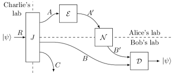
Figure 3: Coherent quantum source-channel coding (coherent QSCC).

After Alice’s transmission, Bob is in possession of the state $\mathcal{N}(\mathcal{E}(\textnormal{Tr}_{C}(J{\left|{\psi}\right\rangle\left\langle{\psi}\right|}J^{\dagger})))$. In order to recover $\left|{\psi}\right\rangle$, Bob must perform some operation that converts the channel $\rho\to\mathcal{N}(\mathcal{E}(\textnormal{Tr}_{C}(J\rho J^{\dagger})))$ into the identity channel. The Kraus operators of this channel are $\{(N_{k}E_{j}\otimes I_{B}\otimes\left\langle{l}\right|_{C})J\}_{jkl}\subseteq\mathcal{L}(R\to B\otimes B^{\prime})$. By the Knill–Laflamme error correction condition [22], recovery of $\left|{\psi}\right\rangle$ is possible if and only if, $\forall j,j^{\prime},k,k^{\prime},l,l^{\prime}$,

$$J^{\dagger}\left(E_{j}^{\dagger}N_{k}^{\dagger}N_{k^{\prime}}E_{j^{\prime}}\otimes I_{B}\otimes\left|{l}\right\rangle\left\langle{l^{\prime}}\right|_{C}\right)J\in\mathbb{C}I.$$ (20)

An operator is proportional to $I$ if and only if it is orthogonal to all trace free operators, so this becomes

$$\phantom{\iff}\left<J^{\dagger}\left(E_{j}^{\dagger}N_{k}^{\dagger}N_{k^{\prime}}E_{j^{\prime}}\otimes I_{B}\otimes\left|{l}\right\rangle\left\langle{l^{\prime}}\right|_{C}\right)J,X\right>=0$$

$$\hskip 100.00015pt\forall j,j^{\prime},k,k^{\prime},l,l^{\prime},\forall X\in Q_{n}$$

$$\iff\left<E_{j^{\prime}}\textnormal{Tr}_{B}\{\left\langle{l^{\prime}}\right|_{C}JXJ^{\dagger}\left|{l}\right\rangle_{C}\}E_{j}^{\dagger},N_{k^{\prime}}^{\dagger}N_{k}\right>=0$$

$$\hskip 100.00015pt\forall j,j^{\prime},k,k^{\prime},l,l^{\prime},\forall X\in Q_{n}$$

$$\iff E\cdot\textnormal{Tr}_{BC}\{\mathcal{L}(C)JQ_{n}J^{\dagger}\}\cdot E^{\dagger}\subseteq(N^{\dagger}N)^{\perp}.$$

Or, using the terminology of homomorphisms,

Theorem 16.

There is a zero-error strategy for coherent QSCC (Fig. 3) if and only if $S\to T$ where $T$ is the distinguishability graph of $\mathcal{N}$, given by (9), and $S$ is the characteristic graph of the source, given by

$$S=\textnormal{Tr}_{BC}\{\mathcal{L}(C)JQ_{n}J^{\dagger}\}$$ (21)

where $n=\dim(R)$.

This differs from Theorem 14 only in the replacement of $K_{n}$ by $Q_{n}$. As before, if Alice and Bob are allowed to make use of an entanglement resource the condition becomes $S\stackrel{{\scriptstyle*}}{{\to}}T$ rather than $S\to T$.

We give some examples.

• Teleportation. Take $J=I_{A_{1}}\otimes\left|{\lambda}\right\rangle_{A_{2}B}$ where $I$ is the identity operator (i.e. the referee directly gives $\left|{\psi}\right\rangle$ to Alice) and $\left|{\lambda}\right\rangle$ is an entanglement resource. Take $\mathcal{N}$ to be a perfect classical channel. By Theorem 16 teleportation is possible if and only if $Q_{m}\otimes\textnormal{Tr}_{B}\{{\left|{\lambda}\right\rangle\left\langle{\lambda}\right|}\}\to K_{n}$ where $m$ is the dimension of the state to be teleported and $n$ is the dimension of the classical channel. The well known bound $m^{2}\leq n$ for teleportation gives $(Q_{m}\stackrel{{\scriptstyle*}}{{\to}}K_{n}\iff m^{2}\leq n)$. In other words, $\omega_{q*}(K_{m^{2}})=m$ and $\chi_{*}(Q_{m})=m^{2}$.

• Zero-error one-shot quantum communication capacity. Take $\mathcal{N}$ to be a noisy channel, and take $J:R\to A$ to be the identity operator (i.e. the referee gives $\left|{\psi}\right\rangle$ directly to Alice, and Bob gets no input). It is possible to send $\log m$ error-free qubits though $\mathcal{N}$ if and only if $Q_{m}\to(N^{\dagger}N)^{\perp}$. By definition, $m\leq\alpha_{q}(N^{\dagger}N)$. If Alice and Bob can use an entangled state, these conditions become $Q_{m}\stackrel{{\scriptstyle*}}{{\to}}(N^{\dagger}N)^{\perp}$ and $m\leq\alpha_{q*}(N^{\dagger}N)$.

• Suppose Alice and Bob each have a share of a quantum state that has been cloned in the standard basis. That is to say, suppose $J=\sum_{x=1}^{n}\left|{xx}\right\rangle_{AB}\left\langle{x}\right|_{R}$. Can Alice send a classical message to Bob such that Bob may reconstruct the original quantum state? The characteristic graph of this source (call it $S$) is the space of trace-free diagonal matrices. Conjugating by the Fourier matrix yields a subspace of $K_{n}$. So the Fourier transform is a homomorphism $S\to K_{n}$; indeed a classical message does suffice.

• Imagine that Alice tries to send a quantum message to Bob, but part of the signal bounces back. This can be modeled by a channel $\mathcal{J}:\mathcal{L}(R)\to\mathcal{L}(A)\otimes\mathcal{L}(B)$. Alice must now send a second message though a second channel $\mathcal{N}$ in order to allow Bob to reconstruct the original message. This is exactly the setup depicted in Fig. 3, with Charlie being Alice and $J$ being the Stinespring isometry of $\mathcal{J}$.

• Correction of algebras. Suppose instead of transmitting $\left|{\psi}\right\rangle$ perfectly, one needs only that some $C^{*}$-algebra of observables $\mathcal{A}$ be preserved (i.e. the receiver can do any POVM measurement with elements from $\mathcal{A}$). This reduces to discrete QSCC when $\mathcal{A}$ consists of the diagonal operators. By theorem 2 of [23], this problem is analyzed via a straightforward modification of the Knill–Laflamme condition: $\mathbb{C}I$ in (20) should be replaced by the space of operators that commute with everything in $\mathcal{A}$ (the commutant of $\mathcal{A}$); Theorem 16 is modified by replacing $Q_{n}$ with the space perpendicular to the commutant of $\mathcal{A}$. Theorem 14 is recovered by taking $\mathcal{A}$ to consist of the diagonal operators.

• Consider discrete QSCC with the inputs $\rho_{1},\rho_{2},\rho_{3},\rho_{4}$ being the four Bell states (or even three of the four). The characteristic graph is $Q_{2}$. This is the same as the graph for coherent QSCC with the goal being for Alice to transmit an arbitrary qubit to Bob ($J:R\to A$ is the identity operator). Since the characteristic graphs are the same for the two problems, they require the same communication resources.

Quantity	Interpretation
$K_{n}=\{M\in\mathcal{L}(\mathbb{C}^{n}):M_{ii}=0\}$	Classical complete graph. The set of $n\times n$ matrices with zeros down the diagonal.
$Q_{n}=(\mathbb{C}I_{n})^{\perp}$	Quantum complete graph. The set of trace-free $n\times n$ matrices.
$N=\textnormal{span}\{N_{i}\}$	Span of Kraus operators for channel $\mathcal{N}$.
$N^{\dagger}N=\textnormal{span}\{N_{i}^{\dagger}N_{j}\}$	Confusability graph of channel $\mathcal{N}$.
$(N^{\dagger}N)^{\perp}$	Distinguishability graph of channel $\mathcal{N}$.
$S\to T\iff ESE^{\dagger}\subseteq T$ with $E$ span of Kraus operators	Graph homomorphism. Source with characteristic graph $S$ can be transmitted using channel with distinguishability graph $T$.
4.5cm $S\stackrel{{\scriptstyle*}}{{\to}}T\iff(\exists\Lambda\succ 0$
s.t. $S\otimes\Lambda\to T)$	Entanglement assisted homomorphism. As before, but sender and receiver share an entanglement resource.
$\omega(S)=\max\{n:K_{n}\to S\}$	Clique number. One-shot classical capacity of channel with distinguishability graph $S$ is $\log\omega(S)$.
$\omega_{q}(S)=\max\{n:Q_{n}\to S\}$	Quantum clique number. One-shot quantum capacity of channel with distinguishability graph $S$ is $\log\omega(S)$.
$\alpha(S)=\omega(S^{\perp})$	Independence number. One-shot classical capacity of channel with confusability graph $S$ is $\log\alpha(S)$.
$\alpha_{q}(S)=\omega_{q}(S^{\perp})$	Quantum independence number. One-shot quantum capacity of channel with confusability graph $S$ is $\log\alpha(S)$.
$\chi(S)=\min\{n:S\to K_{n}\}$	Chromatic number. Source with characteristic graph $S$ can be transmitted using $\log\chi(S)$ classical bits.
$\chi_{q}(S)=\min\{n:S\to Q_{n}\}$	Quantum chromatic number. Source with characteristic graph $S$ can be transmitted using $\log\chi_{q}(S)$ qubits. For classical graphs this equals the orthogonal rank.
$\omega_{*}$, $\omega_{q*}$, $\alpha_{*}$, $\alpha_{q*}$, $\chi_{*}$, $\chi_{q*}$	Entanglement assisted quantities. Replace $\to$ with $\stackrel{{\scriptstyle*}}{{\to}}$ in above definitions. Relevant when sender and receiver share an entanglement resource.

TABLE I: Basic definitions used in this paper, and their interpretations. See Definition 7 for the full definition of $S\to T$. See Theorems 14 and 16 for the definition of characteristic graph.

Lemma 2 of [2] states that every non-commutative graph containing the identity is the confusability graph of some channel (equivalently, every trace-free non-commutative graph is the distinguishability graph of some channel). A similar statement holds for sources.

Theorem 17.

Every non-commutative graph $S$ is the characteristic graph for discrete QSCC with only two inputs (i.e. $\rho_{0}$ and $\rho_{1}$).

Proof.

Let $S\in\mathcal{L}(A)$ be a non-commutative graph and let $\{S_{x}\}_{x\in X}$ be a basis of $S$, with each $S_{x}$ being Hermitian. That such a Hermitian basis always exists is shown in [2]. Without loss of generality, assume that each $S_{x}$ is normalized under the Frobenius norm. Let $(S_{x})_{ij}$ be the entries of matrix $S_{x}$ and define $\left|{S_{x}}\right\rangle=\sum_{ij}(S_{x})_{ij}\left|{i}\right\rangle_{A}\left|{j}\right\rangle_{B}$. Also define $\left|{\Phi}\right\rangle=\dim(A)^{-1/2}\sum_{i}\left|{i}\right\rangle_{A}\otimes\left|{i}\right\rangle_{B}$. Consider discrete QSCC with sources $\rho_{i}=\textnormal{Tr}_{C}\{{\left|{\psi_{i}}\right\rangle\left\langle{\psi_{i}}\right|}\}$ for $i\in\{0,1\}$ with $\left|{\psi_{i}}\right\rangle\in A\otimes B\otimes B^{\prime}\otimes C$ defined by

$$\left|{\psi_{0}}\right\rangle ={\lvert X\rvert}^{-1/2}\sum_{x}\left|{\Phi}\right\rangle\otimes\left|{x}\right\rangle_{B^{\prime}}\otimes\left|{x}\right\rangle_{C}$$

$$\left|{\psi_{1}}\right\rangle ={\lvert X\rvert}^{-1/2}\sum_{x}\left|{S_{x}}\right\rangle\otimes\left|{x}\right\rangle_{B^{\prime}}\otimes\left|{x}\right\rangle_{C}$$

Alice receives subsystem $A$ and Bob receives subsystems $B\otimes B^{\prime}$. Subsystem $C$ goes to the environment. As per Theorem 14, the characteristic graph is

$$S =\textnormal{Tr}_{BB^{\prime}C}\{\mathcal{L}(C)\left|{\psi_{1}}\right\rangle\left\langle{\psi_{0}}\right|\}+\textrm{h.c.}$$

$$=\textnormal{span}_{x}\{\textnormal{Tr}_{B}(\left|{S_{x}}\right\rangle\left\langle{\Phi}\right|)\}+\textrm{h.c.}$$

$$=\textnormal{span}_{x}\{S_{x}\}+\textrm{h.c.}=S$$

where “$+\textrm{h.c.}$” means that the adjoints of the operators are also included in the subspace. ∎

Note that we didn’t require $S$ to be trace-free in Theorem 17; however, if $S$ is not trace-free then source-channel coding will be impossible: $\rho_{0}$ and $\rho_{1}$ would be non-orthogonal and so would not be distinguishable by any measurement.

V $\overline{\vartheta}$ is a homomorphism monotone

We will show that $\overline{\vartheta}$ is monotone under entanglement assisted homomorphisms of non-commutative graphs. This leads to a Lovász sandwich theorem for non-commutative graphs, and a bound on quantum source-channel coding. We begin by showing $\overline{\vartheta}$ to be insensitive to entanglement. Recall that a source having non-commutative graph $S$, combined with an entanglement resource $\left|{\lambda}\right\rangle\in A^{\prime\prime}\otimes B^{\prime\prime}$, yields a composite source with non-commutative graph $S\otimes\Lambda$ where $\Lambda=\textnormal{Tr}_{B^{\prime\prime}}\{{\left|{\lambda}\right\rangle\left\langle{\lambda}\right|}\}$.

Lemma 18.

Let $S$ be a trace-free non-commutative graph. Let $\Lambda$ be a positive operator. Then $\overline{\vartheta}(S)=\overline{\vartheta}(S\otimes\Lambda)$.

Proof.

Suppose $S\subseteq\mathcal{L}(A)$ and $\Lambda\in\mathcal{L}(B)$. By (10) we have

$$\overline{\vartheta}(S) =\max\{\left\lVert I+T\right\rVert:T\in S\otimes\mathcal{L}(\mathbb{C}^{m}),$$

$$\qquad I+T\succeq 0\}$$ (22)

$$\overline{\vartheta}(S\otimes\Lambda) =\max\{\left\lVert I+T\right\rVert:T\in S\otimes\Lambda\otimes\mathcal{L}(\mathbb{C}^{n}),$$

$$\qquad I+T\succeq 0\}.$$ (23)

In [1] is it shown that the ancillary space can be taken to be any dimension at least as large as $\dim(A)$, so in (V)-(V) we may take any values $m\geq\dim(A)$ and $n\geq\dim(A\otimes B)$.

Take $n=\dim(A\otimes B)$ and $m=n\dim(B)$. Any $T$ feasible for (V) is also feasible for (V) since $\Lambda\otimes\mathcal{L}(\mathbb{C}^{n})\subseteq\mathcal{L}(\mathbb{C}^{m})$. So $\overline{\vartheta}(S)\geq\overline{\vartheta}(S\otimes\Lambda)$.

Now take $m=n=\dim(A\otimes B)$. Let $T$ be feasible for (V). Without loss of generality, assume $\left\lVert\Lambda\right\rVert=1$. Then $T^{\prime}:=T\otimes\Lambda$ is feasible for (V). Indeed, $T\succeq-I\implies T^{\prime}\succeq-I$ since $\Lambda\succ 0$ and $\left\lVert\Lambda\right\rVert\leq 1$. Also, $\left\lVert I+T^{\prime}\right\rVert\geq\left\lVert I+T\right\rVert$ since $\Lambda\succ 0$ and $\left\lVert\Lambda\right\rVert\geq 1$. So $\overline{\vartheta}(S\otimes\Lambda)\geq\overline{\vartheta}(S)$. ∎

Before we prove the main theorem, we introduce some notation that will also be used in Section VII. For any (finite dimensional) Hilbert space $A$, define the state

$$\left|{\Phi}\right\rangle_{A}=\sum_{i}\left|{i}\right\rangle_{A}\otimes\left|{i}\right\rangle_{A^{\prime}}.$$ (24)

where $A^{\prime}$ is another Hilbert space of the same dimension as $A$. Note that this provides an isomorphism between $A$ and the dual space of $A^{\prime}$ via the action $\left|{\psi}\right\rangle_{A}\to\left\langle{\Phi}\right|(\left|{\psi}\right\rangle_{A}\otimes I_{A^{\prime}})$. A bar over an operator denotes entrywise complex conjugation in the standard basis (i.e. the basis used in (24)). Additionally, the bar will be understood to move an operator to the primed spaces (or from primed to unprimed). For example, if $J:A\to B\otimes C$ then $\overline{J}:A^{\prime}\to B^{\prime}\otimes C^{\prime}$ is equal to

$$\overline{J}=\textnormal{Tr}_{BC}\{\left|{\Phi}\right\rangle_{BC}\left\langle{\Phi}\right|_{A}J^{\dagger}\}.$$ (25)

We now prove the main theorem of this section: that $\overline{\vartheta}$ is monotone under entanglement assisted homomorphisms. Such an inequality was already known for classical graphs [12].

Theorem 19.

Let $S$ and $T$ be trace-free non-commutative graphs. If $S\to T$ or $S\stackrel{{\scriptstyle*}}{{\to}}T$ then $\overline{\vartheta}(S)\leq\overline{\vartheta}(T)$.

Proof.

If we prove monotonicity under $S\to T$ then monotonicity under $S\stackrel{{\scriptstyle*}}{{\to}}T$ follows. Indeed, if $S\stackrel{{\scriptstyle*}}{{\to}}T$ then there is a $\Lambda\succ 0$ such that $S\otimes\Lambda\to T$. Supposing that $\overline{\vartheta}$ is monotone under (non-entanglement assisted) homomorphisms, we have $\overline{\vartheta}(S\otimes\Lambda)\leq\overline{\vartheta}(T)$. Lemma 18 then gives $\overline{\vartheta}(S)\leq\overline{\vartheta}(T)$.

We now show that $S\to T$ implies $\overline{\vartheta}(S)\leq\overline{\vartheta}(T)$. This can be seen as a consequence of corollaries from [1]. Let $S\subseteq\mathcal{L}(A)$ and $T\subseteq\mathcal{L}(B)$ be trace-free non-commutative graphs with $S\to T$. By Definition 7 there is a Hilbert space $C$ and an isometry $J:A\to B\otimes C$ such that $J^{\dagger}(T^{\perp}\otimes\mathcal{L}(C))J\subseteq S^{\perp}$. Then

$$\tilde{\vartheta}(T^{\perp}) =\tilde{\vartheta}(T^{\perp})\tilde{\vartheta}(\mathcal{L}(C)) \tilde{\vartheta}(\mathcal{L}(C))=1$$ (Since )

$$=\tilde{\vartheta}(T^{\perp}\otimes\mathcal{L}(C))$$ (Corollary 10 of [1])

$$\geq\tilde{\vartheta}(J^{\dagger}(T^{\perp}\otimes\mathcal{L}(C))J)$$ (Corollary 11 of [1])

$$\geq\tilde{\vartheta}(S^{\perp}).$$ (Corollary 11 of [1])

We present also a more direct proof, since this can later be generalized for the $\overline{\vartheta}^{\prime}_{\mathcal{C}}$ and $\overline{\vartheta}^{+}_{\mathcal{C}}$ quantities of Section VII. Let $S\subseteq\mathcal{L}(A)$ and $T\subseteq\mathcal{L}(B)$ be trace-free non-commutative graphs with $S\to T$. By definition there is a CPTP map $\mathcal{E}:\mathcal{L}(A)\to\mathcal{L}(B)$ with Kraus operators $\{E_{i}\}$ such that $E^{\dagger}T^{\perp}E\subseteq S^{\perp}$ where $E=\textnormal{span}\{E_{i}\}$. Let $J:A\to B\otimes C$ be the Stinespring isometry for the channel $\mathcal{E}$, so that $J=\sum_{i}\left|{i}\right\rangle_{C}E_{i}$. Let $\overline{J}:A^{\prime}\to B^{\prime}\otimes C^{\prime}$ be the entrywise complex conjugate of $J$. Recall that $\overline{J}$ takes the form (25).

Let $Y^{\prime}\subseteq\mathcal{L}(B)\otimes\mathcal{L}(B^{\prime})$ be an optimal solution for (11) for $\overline{\vartheta}(T)$. Define $Y\subseteq\mathcal{L}(A)\otimes\mathcal{L}(A^{\prime})$ as

$$Y =\sum_{ij}(E_{i}\otimes\overline{E}_{i})^{\dagger}Y^{\prime}(E_{j}\otimes\overline{E}_{j})$$

$$=(J\otimes\overline{J})^{\dagger}(\left|{\Phi}\right\rangle_{C}\otimes Y^{\prime}\otimes\left\langle{\Phi}\right|_{C})(J\otimes\overline{J}).$$ (26)

We have that

$$Y^{\prime}\in T^{\perp}\otimes\mathcal{L}(B^{\prime}) \implies Y\in E^{\dagger}T^{\perp}E\otimes\overline{E}^{\dagger}\mathcal{L}(B^{\prime})\overline{E}$$

$$\implies Y\in S^{\perp}\otimes\mathcal{L}(A^{\prime}).$$ (27)

Dirac notation becomes unworkable with so many Hilbert spaces, so we will make use of diagrams similar to those of [24] (such diagrams have been used for example in [25, 26]). Operators and states are denoted by labeled boxes and multiplication (or traces or tensor contraction) by wires. This is very much like standard quantum circuits, except that the diagram has no interpretation of time ordering. Wires have an arrow pointing away from the ket space and towards the bra space, and are labeled with the corresponding Hilbert space. Labeled circles represent the transposer operators (24):

With this notation, (26) becomes

(28)

The operator $(J\otimes\overline{J})^{\dagger}(\left|{\Phi}\right\rangle_{C}\otimes I_{BB^{\prime}})$ turns the transposer $\left|{\Phi}\right\rangle_{B}$ into $\left|{\Phi}\right\rangle_{A}$:

$$(J\otimes\overline{J})^{\dagger}(\left|{\Phi}\right\rangle_{C}\otimes\left|{\Phi}\right\rangle_{B}) =(J^{\dagger}\otimes\overline{J}^{\dagger})(\left|{\Phi}\right\rangle_{C}\otimes\left|{\Phi}\right\rangle_{B})$$

$$=(J^{\dagger}J\otimes I)\left|{\Phi}\right\rangle_{A}=\left|{\Phi}\right\rangle_{A}.$$ (29)

With diagrams, the same derivation is written as in Fig. 4.

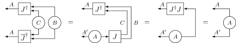
Figure 4: Graphical representation of (29).

Consequently we have $Y^{\prime}\succeq{\left|{\Phi}\right\rangle\left\langle{\Phi}\right|}_{B}\implies Y\succeq{\left|{\Phi}\right\rangle\left\langle{\Phi}\right|}_{A}$ so $Y$ is feasible for (11) for $\overline{\vartheta}(S)$. To get $\overline{\vartheta}(S)\leq\overline{\vartheta}(T)$ it remains only to show $\left\lVert\textnormal{Tr}_{A}Y\right\rVert\leq\left\lVert\textnormal{Tr}_{B}Y^{\prime}\right\rVert$. Let $\rho\in\mathcal{L}(A^{\prime})$ be a density operator achieving $\textnormal{Tr}\{(I_{A}\otimes\rho)Y\}=\left\lVert\textnormal{Tr}_{A}Y\right\rVert$. Plugging (28) (the definition of $Y$) into $\textnormal{Tr}\{(I_{A}\otimes\rho)Y\}$ gives the diagram of Fig. 5.

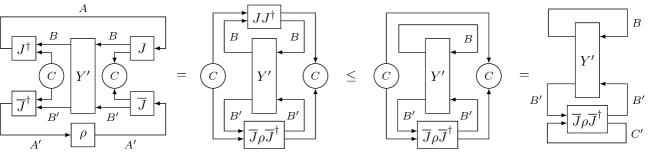
Figure 5: Graphical representation of (30).

The first equality involves only a rearrangement of the diagram. The inequality follows from the fact that $JJ^{\dagger}\preceq I_{BC}$ (since $JJ^{\dagger}$ is a projector) and the rest of the diagram represents a positive semidefinite operator. The last equality uses $\textnormal{Tr}_{C}\{{\left|{\Phi}\right\rangle\left\langle{\Phi}\right|}_{C}\}=I_{C^{\prime}}$. The same derivation can be written in equations as

$$\textnormal{Tr}_{AA^{\prime}}\{(I_{A}\otimes\rho)Y\}$$

$$=\textnormal{Tr}_{AA^{\prime}}\{(I_{A}\otimes\rho)(J\otimes\overline{J})^{\dagger}(\left|{\Phi}\right\rangle_{C}\otimes Y^{\prime}\otimes\left\langle{\Phi}\right|_{C})(J\otimes\overline{J})\}$$

$$=\textnormal{Tr}_{BB^{\prime}CC^{\prime}}\{(JJ^{\dagger}\otimes\overline{J}\rho\overline{J}^{\dagger})(\left|{\Phi}\right\rangle_{C}\otimes Y^{\prime}\otimes\left\langle{\Phi}\right|_{C})\}$$

$$\leq\textnormal{Tr}_{BB^{\prime}CC^{\prime}}\{(I_{BC}\otimes\overline{J}\rho\overline{J}^{\dagger})(\left|{\Phi}\right\rangle_{C}\otimes Y^{\prime}\otimes\left\langle{\Phi}\right|_{C})\}$$

$$=\textnormal{Tr}_{BB^{\prime}C^{\prime}}\{(I_{B}\otimes\overline{J}\rho\overline{J}^{\dagger})(Y^{\prime}\otimes I_{C^{\prime}})\}.$$ (30)

Since $\overline{J}$ is an isometry, $\textnormal{Tr}_{C^{\prime}}\{\overline{J}\rho\overline{J}^{\dagger}\}$ is a density operator. So (30) is bounded from above by $\left\lVert\textnormal{Tr}_{B}Y^{\prime}\right\rVert$ and we have $\left\lVert\textnormal{Tr}_{A}Y\right\rVert\leq\left\lVert\textnormal{Tr}_{B}Y^{\prime}\right\rVert$ as desired. ∎

An immediate corollary is that $\overline{\vartheta}$ satisfies a sandwich theorem analogous to (6).

Corollary 20.

Let $S$ be a trace-free non-commutative graph. Then

1. $\omega_{*}(S)\leq\overline{\vartheta}(S)\leq\chi_{*}(S)$.

2. $\omega_{q*}(S)\leq\sqrt{\overline{\vartheta}(S)}\leq\chi_{q*}(S)$.

Proof.

This follows from applying Theorem 19 to Definition 15 and using the fact that $\overline{\vartheta}(K_{n})=n$ and $\overline{\vartheta}(Q_{n})=n^{2}$. For example, $\omega_{*}(S)$ is the greatest $n$ such that $K_{n}\stackrel{{\scriptstyle*}}{{\to}}S$. By Theorem 19 we have $\overline{\vartheta}(K_{n})\leq\overline{\vartheta}(S)$. Since $\overline{\vartheta}(K_{n})=n$ this gives $n\leq\overline{\vartheta}(S)$.

That $\overline{\vartheta}(K_{n})=n$ and $\overline{\vartheta}(Q_{n})=n^{2}$ is not hard to work out, and is proved in [1]. ∎

The bound on $\omega_{*}(S)$ and $\omega_{q*}(S)$ was shown already in [1], although it was stated in terms of $\alpha_{*}$ and $\alpha_{q*}$. The bound on $\chi_{*}(S)$ and $\chi_{q*}(S)$ is new, although the bound on $\chi_{*}(S)$ was known already for classical graphs [11]. Note that, since for example $\omega(S)\leq\omega_{*}(S)$, we also have the weaker sandwich theorem $\omega(S)\leq\overline{\vartheta}(S)\leq\chi(S)$ and $\omega_{q}(S)\leq\sqrt{\overline{\vartheta}(S)}\leq\chi_{q}(S)$.

This bound $\sqrt{\overline{\vartheta}(S)}\leq\chi_{q}(S)$ is not particularly tight when $S$ corresponds to a classical graph $G$, for the following reason. In such cases $\chi_{q}(S)=\xi(G)$, the orthogonal rank. But it is known that $\overline{\vartheta}(S)=\overline{\vartheta}(G)\leq\xi(G)$ [20], so in this case the square root over $\overline{\vartheta}$ is unnecessary. The necessity of the square root arises from the possibility of dense coding, since we are bounding the entanglement assisted quantities in Corollary 20. Notice that $\omega_{q*}(S)=\left\lfloor\sqrt{\omega_{*}(S)}\right\rfloor$ and $\chi_{q*}(S)=\left\lceil\sqrt{\chi_{*}(S)}\right\rceil$ since a quantum channel of dimension $n$ can simulate a classical channel of dimension $n^{2}$, and teleportation can do the reverse.

The square root in Corollary 20 could be eliminated by defining a different generalization of Lovász’s $\overline{\vartheta}$ that is monotone under homomorphisms and which takes the value $n$ on the graph $Q_{n}$. Such a quantity would necessarily not be monotone under entanglement assisted homomorphisms, since $Q_{2}\stackrel{{\scriptstyle*}}{{\to}}K_{4}$. Finding such a quantity is left as an open question.

Theorem 19 can be applied to give bounds for all of the examples in Section IV. Two are especially noteworthy: Theorem 19 gives the well known bounds $n\leq m^{2}$ for dense coding and $n^{2}\leq m$ for teleportation (where $n$ is the dimension of the source and $m$ is the dimension of the channel).

VI Graph products and block coding

Consider the problem of sending several parallel sources using several parallel channels. In general these several sources (as well as the channels) could all be distinct, and we will in fact consider this. In the special case where the sources are identical, as well as the channels, one may ask how many channel uses are required for each instance of the source. This is known as the cost rate. For classical sources and channels, we saw already (Proposition 5) that a bound on cost rate is given in terms of the Lovász $\overline{\vartheta}$ number. The goal of this section is to prove an analogous bound in the case of quantum sources and channels. To build this theory, we begin with an investigation of the classical case.

Consider two channels $\mathcal{N}(v|s)$ and $\mathcal{N}^{\prime}(v^{\prime}|s^{\prime})$ having distinguishability graphs $H$ and $H^{\prime}$. It is not hard to see that the composite channel $\mathcal{N}^{\prime\prime}(v,v^{\prime}|s,s^{\prime})=\mathcal{N}(v|s)\mathcal{N}^{\prime}(v^{\prime}|s^{\prime})$ has a distinguishability graph with vertices $V(H)\times V(H^{\prime})$ and edges

$$(x,x^{\prime})\sim(y,y^{\prime})\iff(x\sim y)\textrm{ or }(x^{\prime}\sim y^{\prime}).$$ (31)

This is known as the disjunctive product, denoted $H*H^{\prime}$. If $n$ identical copies of $\mathcal{N}$ are used in parallel, the resulting composite channel will have distinguishability graph $H^{*n}=H*H*\dots*H$. Since the one-shot capacity of a channel is $\log\omega(H)$ bits, the capacity (per-channel use) of $n$ parallel channels is $\frac{1}{n}\log\omega(H^{*n})$. The capacity in the limit $n\to\infty$ is known as the Shannon capacity of the channel,

$$C_{0}({\overline{H}})=\lim_{n\to\infty}\frac{1}{n}\log\omega(H^{*n}).$$ (32)

Since $\omega(H^{*n})$ is super-multiplicative, by Fekete’s lemma this limit exists and is equal to the supremum. The complement in the argument of $C_{0}({\overline{H}})$ is because we consider the distinguishability graph rather than the confusability graph, in terms of which $C_{0}$ is typically defined. Since $\overline{\vartheta}(H^{*n})=\overline{\vartheta}(H)^{n}$, it holds that $C_{0}({\overline{H}})\leq\log\overline{\vartheta}(H)$ [20]. In fact this was the original motivation for defining the $\vartheta$ number.

Now consider parallel sources. Recall from Section II that the sources $P(x,u|i)$ we consider are somewhat generalized from what is traditionally considered. The traditional definition is obtained by requiring $P(x,u|i)\neq 0$ only when $x=i$. In this case, the characteristic graphs of parallel sources combine by the strong product [7] which has vertices $V(G)\times V(G^{\prime})$ and edges

$$(x,x^{\prime})\sim(y,y^{\prime})\iff (x\sim y\textrm{ and }x^{\prime}\sim y^{\prime})\textrm{ or }$$

$$(x=y\textrm{ and }x^{\prime}\sim y^{\prime})\textrm{ or }$$

$$(x\sim y\textrm{ and }x^{\prime}=y^{\prime}).$$ (33)

Adapting this to non-commutative graphs is problematic because there is no clear analogue of the condition $x=y$. But already for our generalized sources, which can have $P(x,u|i)\neq 0$ when $x\neq i$, the product rule needs modification.

Consider two parallel sources $P(x,u|i)$ and $P(x^{\prime},u^{\prime}|i^{\prime})$ (these can be over different alphabets) with characteristic graphs $G$ and $G^{\prime}$. Call the combined source $P^{\prime\prime}(x,x^{\prime},u,u^{\prime}|i,i^{\prime}):=P(x,u|i)P(x^{\prime},u^{\prime}|i^{\prime})$. This has characteristic graph $G^{\prime\prime}$ with vertex set $V(G)\times V(G^{\prime})$ and edges given by a generalization of (33). To this end, we introduce a graph $G_{0}$ having the same vertices as $G$ but with edges

$$x\sim_{G_{0}}y\iff\exists u,\exists i \textrm{ s.t.\ }P(x,u|i)P(y,u|i)\neq 0.$$ (34)

$G^{\prime}_{0}$ is defined similarly. If $P(x,u|i)\neq 0$ only when $x=i$ then $G_{0}$ has edges $x\sim_{G_{0}}y\iff x=y$. In other words $G_{0}$ consists only of loops. So (34) can be regarded as a set of generalized loops. We will call the pair $(G,G_{0})$ a graph with generalized loops. We can now compute $G^{\prime\prime}$, the characteristic graph for the composite source:

$$(x,x^{\prime})\sim_{G^{\prime\prime}} (y,y^{\prime})$$

$$\iff \exists u,u^{\prime},\exists(i,i^{\prime})\neq(j,j^{\prime})\textrm{ s.t.\ }$$

$$P^{\prime\prime}(x,x^{\prime},u,u^{\prime}|i,i^{\prime})P^{\prime\prime}(y,y^{\prime},u,u^{\prime}|j,j^{\prime})\neq 0$$

$$\iff (x\sim_{G}y\textrm{ and }x^{\prime}\sim_{G^{\prime}}y^{\prime})\textrm{ or }$$

$$(x\sim_{G_{0}}y\textrm{ and }x^{\prime}\sim_{G^{\prime}}y^{\prime})\textrm{ or }$$

$$(x\sim_{G}y\textrm{ and }x^{\prime}\sim_{G^{\prime}_{0}}y^{\prime}).$$ (35)

And the graph $G^{\prime\prime}_{0}$, defined analogously to (34), has edges

$$(x,x^{\prime})\sim_{G^{\prime\prime}_{0}} (y,y^{\prime})$$

$$\iff \exists u,u^{\prime},\exists i,i^{\prime}\textrm{ s.t.\ }$$

$$P^{\prime\prime}(x,x^{\prime},u,u^{\prime}|i,i^{\prime})P^{\prime\prime}(y,y^{\prime},u,u^{\prime}|i,i^{\prime})\neq 0$$

$$\iff x\sim_{G_{0}}y\textrm{ and }x^{\prime}\sim_{G^{\prime}_{0}}y^{\prime}.$$ (36)

We introduce the notation $(G^{\prime\prime},G^{\prime\prime}_{0})=(G,G_{0})\boxtimes(G^{\prime},G^{\prime}_{0})$ as shorthand for (35)-(36). By induction, $m$ parallel instances of a source yields a characteristic graph $(G,G_{0})^{\boxtimes m}:=(G,G_{0})\boxtimes(G,G_{0})\boxtimes\dots\boxtimes(G,G_{0})$.

For convenience we will abuse notation by treating these ordered pairs as being graphs themselves. For instance, $(G,G_{0})^{\boxtimes m}\to H$ will be taken to mean $G^{\prime}\to H$ where $(G^{\prime},G^{\prime}_{0})=(G,G_{0})^{\boxtimes m}$; similarly $\overline{\vartheta}((G,G_{0})^{\boxtimes m})$ will be taken to mean $\overline{\vartheta}(G^{\prime})$ and $(G,G_{0})^{\boxtimes m}\supseteq G^{\boxtimes m}$ to mean $G^{\prime}\supseteq G^{\boxtimes m}$.

Now we can show that the condition $P(x,u|i)\neq 0$ only when $x=i$ can be dropped in Proposition 5. This is only a slight generalization of [10]. We will later generalize this to quantum sources and quantum channels.

Proposition 21.

Let $P(x,u|i)$ be a classical source and $\mathcal{N}(v|s)$ a classical channel. Let graphs $G$ and $H$ be given by (2) and (1). Then $m$ parallel instances of the source can be sent using $n$ parallel instances of the channel only if

$$\frac{n}{m}\geq\frac{\log\overline{\vartheta}(G)}{\log\overline{\vartheta}(H)}.$$

Proof.

Without loss of generality assume that each $x$ is possible. In other words, assume that for each $x$ there is an $i$ and $u$ such that $P(x,u|i)\neq 0$. Generality is not lost because one can decrease the alphabet associated with $x$, removing values that can never occur. Reducing this alphabet only removes isolated vertices from $G$, and so doesn’t affect the value of $\overline{\vartheta}(G)$. Let $G_{0}$ be defined as in (34). Since each $x$ is possible, this graph has loops on all vertices: $x\sim_{G_{0}}x$ for all $x$.

As per the above discussion, the composite source (consisting of $m$ parallel instances of $P(x,u|i)$) will have characteristic graph $(G,G_{0})^{\boxtimes m}$. Since $G_{0}$ has loops on all vertices, our generalized strong product (35) has at least as many edges as the standard strong product (33). Since $\overline{\vartheta}$ is monotone increasing under addition of edges and is multiplicative under the strong product [27] we have $\overline{\vartheta}((G,G_{0})^{\boxtimes m})\geq\overline{\vartheta}(G^{\boxtimes m})=\overline{\vartheta}(G)^{m}$.

The distinguishability graph of $n$ parallel instances of the channel $\mathcal{N}(v|s)$ is $H^{*n}$. Since $\overline{\vartheta}$ is multiplicative under the disjunctive product [20] we have $\overline{\vartheta}(H^{*n})=\overline{\vartheta}(H)^{n}$. If $m$ parallel sources can be sent via $n$ parallel channels then $(G,G_{0})^{\boxtimes m}\to H^{*n}$. Since $\overline{\vartheta}$ is monotone under homomorphisms,

$$(G,G_{0})^{\boxtimes m}\to H^{*n} \implies\overline{\vartheta}((G,G_{0})^{\boxtimes m})\leq\overline{\vartheta}(H^{*n})$$

$$\implies\overline{\vartheta}(G)^{m}\leq\overline{\vartheta}(H)^{n}$$

$$\implies\frac{n}{m}\geq\frac{\log\overline{\vartheta}(G)}{\log\overline{\vartheta}(H)}.$$

∎

Similar arguments apply for quantum source-channel coding. It is easy to see that the confusability graphs for parallel channels should combine by tensor product since the Kraus operators combine by tensor product. We have been using instead the distinguishability graph, which then combines as $(S^{\perp}\otimes T^{\perp})^{\perp}$. We take this as the definition of disjunctive product:

Definition 22.

Let $S\subseteq\mathcal{L}(A)$ and $T\subseteq\mathcal{L}(B)$ be non-commutative graphs. Their disjunctive product is $S*T=S\otimes\mathcal{L}(B)+\mathcal{L}(A)\otimes T=(S^{\perp}\otimes T^{\perp})^{\perp}$.

When $S$ and $T$ derive from classical graphs this definition is equivalent to (31). We will use the notation $S^{*n}:=S*S*\dots*S$. Analogous to (32), the Shannon capacity of a quantum channel with distinguishability graph $T$ is

$$C_{0}(T^{\perp})=\lim_{n\to\infty}\frac{1}{n}\log\omega(T^{*n})$$

It is known that $\overline{\vartheta}(T)$ is an upper bound on $C_{0}(T^{\perp})$, since $\overline{\vartheta}(T^{*n})=\tilde{\vartheta}((T^{\perp})^{\otimes n})=\overline{\vartheta}(T)^{n}$ [1].

Consider now two parallel sources, with characteristic graphs $S$ and $S^{\prime}$. Analogous to (34) we define $(S,S_{0})$, a non-commutative graph with generalized loops. For discrete QSCC, the subject of Theorem 14, define

$$S =\textnormal{Tr}_{BC}\{\mathcal{L}(C)JK_{r}J^{\dagger}\}$$

$$S_{0} =\textnormal{Tr}_{BC}\{\mathcal{L}(C)JK_{r}^{\perp}J^{\dagger}\}$$ (37)

and for coherent QSCC, the subject of Theorem 16, define

$$S =\textnormal{Tr}_{BC}\{\mathcal{L}(C)JQ_{r}J^{\dagger}\}$$

$$S_{0} =\textnormal{Tr}_{BC}\{\mathcal{L}(C)JQ_{r}^{\perp}J^{\dagger}\}$$

$$=\textnormal{Tr}_{BC}\{\mathcal{L}(C)JJ^{\dagger}\},$$ (38)

where $J:R\to A\otimes B\otimes C$ and $r=\dim(R)$. Analogous to (35)-(36) define the strong product $(S^{\prime\prime},S^{\prime\prime}_{0})=(S,S_{0})\boxtimes(S^{\prime},S^{\prime}_{0})$ as

$$S^{\prime\prime} =(S\otimes S^{\prime})+(S_{0}\otimes S^{\prime})+(S\otimes S^{\prime}_{0})$$

$$S^{\prime\prime}_{0} =S_{0}\otimes S^{\prime}_{0}.$$ (39)

If $S,S_{0},S^{\prime},S^{\prime}_{0}$ correspond to classical graphs $G,G_{0},G^{\prime},G^{\prime}_{0}$ then this product corresponds to the classical graph $(G,G_{0})\boxtimes(G^{\prime},G^{\prime}_{0})$. If $G_{0}$ and $G^{\prime}_{0}$ consist of only loops on each vertex (i.e. $S_{0}=\textnormal{span}\{{\left|{x}\right\rangle\left\langle{x}\right|}\}$ and similarly for $S^{\prime}_{0}$) then this corresponds to $G\boxtimes G^{\prime}$. Define the graph power $(S,S_{0})^{\boxtimes m}$ to be repeated application of (39).

Other graph products could be defined similarly. For example, the Cartesian product of graphs, $G\mathbin{\square}G^{\prime}$ is defined to have edges $(x,x^{\prime})\sim(y,y^{\prime})\iff(x=y\wedge x^{\prime}\sim y^{\prime})\vee(x\sim y\wedge x^{\prime}=y^{\prime})$, so for non-commutative graphs one could define $(S^{\prime\prime},S^{\prime\prime}_{0})=(S,S_{0})\mathbin{\square}(S^{\prime},S^{\prime}_{0})$ with $S^{\prime\prime}=(S_{0}\otimes S^{\prime})+(S\otimes S^{\prime}_{0})$ and $S^{\prime\prime}_{0}=S_{0}\otimes S^{\prime}_{0}$. The complement of a graph has edges $x\not\sim y\wedge x\neq y$, which would have non-commutative analogue $\overline{(S,S_{0})}=(S^{\perp}\setminus S_{0},S_{0})$, assuming $S_{0}\subseteq S^{\perp}$. We will not have occasion to consider such constructions, but mention it as a starting point for possible development of a richer theory of non-commutative graphs. A similar concept was explored in [28]; however, they suggested a specific form of $S_{0}$ in terms of the multiplicative domain of a channel whereas we leave the form of $S_{0}$ to be determined by the application at hand.

As before, we abuse notation and take $(S,S_{0})^{\boxtimes m}\to T$ to mean $S^{\prime}\to T$ where $(S^{\prime},S^{\prime}_{0})=(S,S_{0})^{\boxtimes m}$, and $\overline{\vartheta}((S,S_{0})^{\boxtimes m})$ to mean $\overline{\vartheta}(S^{\prime})$. The strong product (39) indeed corresponds to the characteristic graph of parallel sources:

Theorem 23.

Consider discrete QSCC with two sources $\{\rho_{i}\}_{i\in\{1,\dots,r\}}\subseteq\mathcal{L}(A)\otimes\mathcal{L}(B)$ and $\{\rho^{\prime}_{i}\}_{i\in\{1,\dots,r^{\prime}\}}\subseteq\mathcal{L}(A^{\prime})\otimes\mathcal{L}(B^{\prime})$. As in Theorem 14, for each $i$ let $\left|{\psi_{i}}\right\rangle\in A\otimes B\otimes C$ be a purification of $\rho_{i}$ and define the isometry $J:R\to A\otimes B\otimes C$ with $R=\mathbb{C}^{r}$ as $J=\sum_{i=1}^{r}\left|{\psi_{i}}\right\rangle\left\langle{i}\right|$. Define $\left|{\psi^{\prime}_{i}}\right\rangle$ and $J^{\prime}$ similarly.

Let $(S,S_{0})$ and $(S^{\prime},S^{\prime}_{0})$ be the characteristic graphs (with generalized loops) for these two sources, as defined by (37), and similarly $(S^{\prime\prime},S^{\prime\prime}_{0})$ for the joint source $\{\left|{\psi_{i}}\right\rangle\otimes\left|{\psi^{\prime}_{i^{\prime}}}\right\rangle\}_{i,i^{\prime}}$. Then it holds that $(S^{\prime\prime},S^{\prime\prime}_{0})=(S,S_{0})\boxtimes(S^{\prime},S^{\prime}_{0})$. These two sources can be sent using one copy of the channel $\mathcal{N}$ iff

$$(S,S_{0})\boxtimes(S^{\prime},S^{\prime}_{0})\to T$$ (40)

where $T=(N^{\dagger}N)^{\perp}$.

The analogous statement holds for coherent QSCC, where now $(S,S_{0})$, $(S^{\prime},S^{\prime}_{0})$, and $(S^{\prime\prime},S^{\prime\prime}_{0})$ are defined using (38) rather than (37).

In either case (discrete or coherent QSCC), it is possible to send $m$ copies of a source using $n$ copies of a channel iff

$$(S,S_{0})^{\boxtimes m}\to T^{*n}.$$ (41)

Proof.

We give the proof only for discrete QSCC; the proof for coherent QSCC follows from similar arguments. A state from the joint source will be of the form $\left|{\psi^{\prime\prime}_{ii^{\prime}}}\right\rangle=\left|{\psi_{i}}\right\rangle\otimes\left|{\psi^{\prime}_{i^{\prime}}}\right\rangle$ and the corresponding isometry will be $J^{\prime\prime}=J\otimes J^{\prime}$, so we have (according to (37))

$$S^{\prime\prime} =\textnormal{Tr}_{BB^{\prime}CC^{\prime}}\{\mathcal{L}(C\otimes C^{\prime})J^{\prime\prime}K_{r^{\prime\prime}}J^{\prime\prime{\dagger}}\}$$

$$S^{\prime\prime}_{0} =\textnormal{Tr}_{BB^{\prime}CC^{\prime}}\{\mathcal{L}(C\otimes C^{\prime})J^{\prime\prime}K_{r^{\prime\prime}}^{\perp}J^{\prime\prime{\dagger}}\}$$

where $r^{\prime\prime}=rr^{\prime}=\dim(R)\dim(R^{\prime})$. It is readily verified that $(S^{\prime\prime},S^{\prime\prime}_{0})=(S,S_{0})\boxtimes(S^{\prime},S^{\prime}_{0})$, since

$$K_{r^{\prime\prime}} =K_{r}\otimes K_{r^{\prime}}+K_{r}^{\perp}\otimes K_{r^{\prime}}+K_{r}\otimes K_{r^{\prime}}^{\perp},$$

$$K_{r^{\prime\prime}}^{\perp} =K_{r}^{\perp}\otimes K_{r^{\prime}}^{\perp}.$$

By Theorem 14, the joint source can be sent using a single use of channel $\mathcal{N}$ iff $S^{\prime\prime}\to T$, that is to say iff condition (40) holds.

By induction, $m$ instances of a source can be sent with a single channel use iff $(S,S_{0})^{\boxtimes m}\to T$. Since the distinguishability graph of $n$ copies of the channel is $T^{*n}$, it is possible to send $m$ instances of the source using $n$ instances of the channel iff $(S,S_{0})^{\boxtimes m}\to T^{*n}$. ∎

For classical source-channel coding the amount of communication needed to transmit a joint source is at least as much as is needed for each individual source, since the second source can always be simulated: Alice and Bob can just agree ahead of time on some $x^{\prime}$ and $u^{\prime}$ that can be emitted be the second source. Somewhat surprisingly, this does not necessarily hold for quantum source-channel coding. For example, consider the following two sources. The first source is some classical source for which an entanglement resource ${\left|{\lambda}\right\rangle\left\langle{\lambda}\right|}$ would allow for more efficient transmission. In other words, $\chi(S)$ is large and $\chi_{*}(S)$ is small. Examples of such graphs are given in, e.g. [15]. The second source consists of only a single possible input: ${\left|{\lambda}\right\rangle\left\langle{\lambda}\right|}$. So $S^{\prime}=\varnothing$ and $S^{\prime}_{0}=\mathbb{C}\Lambda$ where $\Lambda=\textnormal{Tr}_{B}\{{\left|{\lambda}\right\rangle\left\langle{\lambda}\right|}\}$. Then the first source requires an amount of communication $\chi(S)$, the second requires no communication (i.e. $\chi(S^{\prime})=1$), but the joint source requires communication $\chi_{*}(S)<\max\{\chi(S),\chi(S^{\prime})\}$.

Entanglement assisted chromatic number does not exhibit this same anomaly. Indeed, the joint source can never be easier to transmit than either of the individual sources since Alice and Bob can always simulate (some particular input from) the second source, by choosing said state ahead of time and adding this to their entanglement resource. For a similar reason, even without entanglement assistance a joint source is not easier to transmit than the individual sources in the case where the individual sources are each capable of producing a product state: Alice and Bob can simulate any of these sources by producing the product state themselves, in order to turn a single source into (a subset of) the joint source.

For classical source-channel coding, we defined the cost rate as the infimum of $n/m$ such that $m$ instances of the source can be transmitted using $n$ instances of the channel. As per the above discussion, this can be achieved iff $(G,G_{0})^{\boxtimes m}\to H^{*n}$, so the cost rate is

$$\lim_{m\to\infty}\frac{1}{m}\min\left\{n:(G,G_{0})^{\boxtimes m}\to H^{*n}\right\}.$$

Cost rate for quantum source-channel coding can be defined similarly,

$$\lim_{m\to\infty}\frac{1}{m}\min\left\{n:(S,S_{0})^{\boxtimes m}\to T^{*n}\right\},$$ (42)

where $(S,S_{0})$ is the characteristic graph of the source (as per (37) or (38)) and $T$ is the distinguishability graph of the channel. Similarly, the entanglement assisted cost rate is

$$\lim_{m\to\infty}\frac{1}{m}\min\left\{n:(S,S_{0})^{\boxtimes m}\stackrel{{\scriptstyle*}}{{\to}}T^{*n}\right\}.$$ (43)

Clearly $\eqref{eq:costrate_nc_ent}\leq\eqref{eq:costrate_nc}$.

In all three cases, by Fekete’s lemma the limit exists and is equal to the infimum, since the $\min\{n:\dots\}$ quantities are sub-multiplicative in $m$. This can be seen as follows: if it is possible to transmit $m_{1}$ instances of the source using $n_{1}$ instances of the channel via one protocol, and $m_{2}$ instances of the source using $n_{2}$ instances of the channel via another protocol, one can transmit $m_{1}+m_{2}$ instances of the source using $n_{1}+n_{2}$ instances of the channel by simply running the two protocols in parallel.

For the classical case, the Lovász $\overline{\vartheta}$ number is multiplicative under the relevant graph products and is a homomorphism monotone, so it leads to a lower bound on the cost rate, Proposition 21. A similar bound applies for quantum source-channel coding, with a caveat. The $\overline{\vartheta}$ quantity is not multiplicative under strong product in general; however, it is when $S_{0}$ and $S^{\prime}_{0}$ contain the identity. So our generalization of Proposition 21 will require $I\in S_{0}$. This happens for example when the states emitted by the source include a maximally entangled state, or product states with Alice’s shares forming a complete orthonormal basis (such as is the case with classical source-channel coding). We have then the following bound on cost rate.

Theorem 24.

Consider a source with characteristic graph $(S,S_{0})$, defined as in (37) for discrete QSCC or as in (38) for coherent QSCC. Consider a noisy quantum channel $\mathcal{N}$ with distinguishability graph $T=(N^{\dagger}N)^{\perp}$. If $I\in S_{0}$ then the entanglement assisted cost rate (43) is lower bounded by $\log\overline{\vartheta}(S)/\log\overline{\vartheta}(T)$.

Proof.

Since $I\in S_{0}$, the $\overline{\vartheta}$ quantity is multiplicative under both strong and disjunctive graph powers, by Lemma 25. Using this fact, and the fact that $\overline{\vartheta}$ is monotone under entanglement assisted homomorphisms, we have

$$\eqref{eq:costrate_nc_ent} \geq\inf_{m\to\infty}\frac{1}{m}\min\left\{n:\overline{\vartheta}((S,S_{0})^{\boxtimes m})\leq\overline{\vartheta}(T^{*n})\right\}$$

$$=\inf_{m\to\infty}\frac{1}{m}\min\left\{n:\overline{\vartheta}(S)^{m}\leq\overline{\vartheta}(T)^{n}\right\}$$

$$=\inf_{m\to\infty}\frac{1}{m}\min\left\{n:\log\overline{\vartheta}(S)/\log\overline{\vartheta}(T)\leq n/m\right\}$$

$$=\log\overline{\vartheta}(S)/\log\overline{\vartheta}(T).$$

∎

We now prove the lemma used in the preceding proof.

Lemma 25.

Let $S$ and $S^{\prime}$ be trace-free non-commutative graphs. Then,

• $\overline{\vartheta}(S*S^{\prime})=\overline{\vartheta}(S)\overline{\vartheta}(S^{\prime})$

• $\overline{\vartheta}((S,S_{0})\boxtimes(S^{\prime},S^{\prime}_{0}))=\overline{\vartheta}(S)\overline{\vartheta}(S^{\prime})$ if $I\in S_{0}$ and $I\in S^{\prime}_{0}$

Proof.

From [1] we have $\tilde{\vartheta}(S^{\perp}\otimes S^{\prime\perp})=\tilde{\vartheta}(S^{\perp})\tilde{\vartheta}(S^{\prime\perp})$. But $(S^{\perp}\otimes S^{\prime\perp})^{\perp}=S*S^{\prime}$, so $\overline{\vartheta}(S*S^{\prime})=\overline{\vartheta}(S)\overline{\vartheta}(S^{\prime})$. Since $(S,S_{0})\boxtimes(S^{\prime},S^{\prime}_{0})\subseteq S*S^{\prime}$ and since $\overline{\vartheta}$ is monotone decreasing under subsets, we have

$$\overline{\vartheta}((S,S_{0})\boxtimes(S^{\prime},S^{\prime}_{0}))\leq\overline{\vartheta}(S*S^{\prime})=\overline{\vartheta}(S)\overline{\vartheta}(S^{\prime}).$$

Let $X$ be an optimal solution to (10) for $\overline{\vartheta}(S)$, from Definition 6. Then $X\in S\otimes\mathcal{L}(B)$ (for some Hilbert space $B$), $I+X\succeq 0$, and $\left\lVert I+X\right\rVert=\overline{\vartheta}(S)$. Similarly, there is an $X^{\prime}\in S^{\prime}\otimes\mathcal{L}(B^{\prime})$, $I+X^{\prime}\succeq 0$, and $\left\lVert I+X^{\prime}\right\rVert=\overline{\vartheta}(S^{\prime})$. Define

$$X^{\prime\prime} =(I_{AB}+X)\otimes(I_{A^{\prime}B^{\prime}}+X^{\prime})-I_{AA^{\prime}BB^{\prime}}.$$

Clearly $I+X^{\prime\prime}\succeq 0$. Also,

$$X^{\prime\prime} =X\otimes X^{\prime}+I_{AB}\otimes X^{\prime}+X\otimes I_{A^{\prime}B^{\prime}}$$

$$\in[S\otimes S^{\prime}+I_{A}\otimes S^{\prime}+S\otimes I_{A^{\prime}}]\otimes\mathcal{L}(BB^{\prime})$$

$$\subseteq[S\otimes S^{\prime}+S_{0}\otimes S^{\prime}+S\otimes S^{\prime}_{0}]\otimes\mathcal{L}(BB^{\prime})$$

$$=[(S,S_{0})\boxtimes(S^{\prime},S^{\prime}_{0})]\otimes\mathcal{L}(BB^{\prime}).$$

So $X^{\prime\prime}$ is feasible for (10) for $\overline{\vartheta}((S,S_{0})\boxtimes(S^{\prime},S^{\prime}_{0}))$. Therefore

$$\overline{\vartheta}((S,S_{0})\boxtimes(S^{\prime},S^{\prime}_{0})) \geq\left\lVert I+X^{\prime\prime}\right\rVert$$

$$=\left\lVert(I+X)\otimes(I+X^{\prime})\right\rVert$$

$$=\overline{\vartheta}(S)\overline{\vartheta}(S^{\prime}).$$

∎

VII Schrijver and Szegedy numbers

In this section we will provide a generalization to non-commutative graphs for two quantities related to Lovász’s $\vartheta$: Schrijver’s $\vartheta^{\prime}$ and Szegedy’s $\vartheta^{+}$. Schrijver’s number comes from adding extra constraints to the maximization program for $\vartheta$, yielding a smaller value; Szegedy’s number comes from adding extra constraints to the minimization (dual) program for $\vartheta$, yielding a larger value. We will consider the complimentary quantities $\overline{\vartheta}^{\prime}(G)=\vartheta^{\prime}({\overline{G}})$ and $\overline{\vartheta}^{+}(G)=\vartheta^{+}({\overline{G}})$. These are homomorphism monotones in the same sense that $\overline{\vartheta}$ is [14]; therefore they satisfy the sandwich theorem

$$\omega(G)\leq\overline{\vartheta}^{\prime}(G)\leq\overline{\vartheta}(G)\leq\overline{\vartheta}^{+}(G)\leq\chi(G).$$

These quantities are not suitable for bounding asymptotic channel capacity or cost rate for source-channel coding because they are not multiplicative under the appropriate graph products [12].

For classical graphs these quantities have been shown to be monotone under entanglement assisted homomorphisms [12]. Strangely enough, our generalization to non-commutative graphs will yield quantities monotone under homomorphisms but not under entanglement assisted homomorphisms. For classical graphs the gap between $\overline{\vartheta}^{\prime}(G)$ and $\overline{\vartheta}^{+}(G)$ tends to be small or, often, zero. For non-commutative graphs the gap tends to be much more extreme, sometimes infinite, even for random graphs of small dimension. After developing basic properties of these quantities we will show how they can be used to reproduce some results from the literature regarding entanglement assisted activation of one-shot channel capacity and impossibility of one-way LOCC measurement of entangled states. Also we will provide a channel for which maximally entangled states are not sufficient for achieving the entanglement assisted one-shot capacity.

The classical quantities are defined as follows [20, 27, 29, 30, 31].

Definition 26.

The Lovász, Schrijver, and Szegedy numbers of the complement of a graph, $\overline{\vartheta}(G)$, $\overline{\vartheta}^{\prime}(G)$, and $\overline{\vartheta}^{+}(G)$, are defined by the following dual (and equivalent) semidefinite programs. All matrices are either real or complex (it doesn’t matter), $J$ is the all-ones matrix, and $\mathcal{N}$ is the cone of symmetric entrywise non-negative matrices. Take $S=\textnormal{span}\{\left|{x}\right\rangle\left\langle{y}\right|:x\sim y\}$ and $S_{0}=\textnormal{span}\{\left|{x}\right\rangle\left\langle{x}\right|:x\in V(G)\}$ (the diagonal matrices).

$$\overline{\vartheta}(G) =\max\left<B,J\right> B\succeq 0,\textnormal{Tr}B=1,$$ s.t.

$$B\in S+S_{0}$$ (44)

$$\overline{\vartheta}^{\prime}(G) =\max\left<B,J\right> B\succeq 0,\textnormal{Tr}B=1,$$ s.t.

$$B\in S+S_{0},B\in\mathcal{N}$$ (45)

$$\overline{\vartheta}^{+}(G) =\max\left<B,J\right> B\succeq 0,\textnormal{Tr}B=1,$$ s.t.

$$B+L\in S+S_{0},L\in\mathcal{N}$$ (46)

$$\overline{\vartheta}(G) =\min\lambda Z\succeq J,(Z_{ii}=\lambda\textrm{ for all }i),$$ s.t.

$$Z\in S^{\perp}$$ (47)

$$\overline{\vartheta}^{\prime}(G) =\min\lambda Z\succeq J,(Z_{ii}=\lambda\textrm{ for all }i),$$ s.t.

$$Z+L\in S^{\perp},L\in\mathcal{N}$$ (48)

$$\overline{\vartheta}^{+}(G) =\min\lambda Z\succeq J,(Z_{ii}=\lambda\textrm{ for all }i),$$ s.t.

$$Z\in S^{\perp},Z\in\mathcal{N}$$ (49)

The constraint $B\in\mathcal{N}$ that is added to (44) to yield (45) has the following justification. Suppose that $W\subseteq V(G)$ is a clique. Then the matrix

$$B_{ij}=\begin{cases}1/{\lvert W\rvert}&\textrm{if }i,j\in W\\ 0&\textrm{otherwise}\end{cases}$$

is a feasible solution to (44) with value ${\lvert W\rvert}$. So $\omega(G)\leq\overline{\vartheta}(G)$. But $B\in\mathcal{N}$, so this condition can be added to the maximization program to yield a potentially smaller quantity $\overline{\vartheta}^{\prime}(G)$ that still upper bounds $\omega(G)$. Similarly, if $f:V(G)\to\{1,\dots,m\}$ is a proper coloring of $G$ then

$$Z_{ij}=\begin{cases}m&\textrm{if }f(i)=f(j)\\ 0&\textrm{otherwise}\end{cases}$$

is feasible for (47) with value $\chi(G)$, so $\overline{\vartheta}(G)\geq\chi(G)$. Since this satisfies $Z\in\mathcal{N}$, adding this condition to the minimization program gives a quantity $\overline{\vartheta}^{+}(G)$ still lower bounding $\chi(G)$. We will follow this sort of strategy to create analogues of $\overline{\vartheta}^{\prime}$ and $\overline{\vartheta}^{+}$ for non-commutative graphs.

The primal program for $\overline{\vartheta}$ can be written [1]

$$\overline{\vartheta}(S)=\max \;\left\langle{\Phi}\middle|{I\otimes\rho+T}\middle|{\Phi}\right\rangle$$

s.t. $$\;\rho\succeq 0,\textnormal{Tr}\rho=1,$$

$$\;I\otimes\rho+T\succeq 0,$$

$$\;T\in S\otimes\mathcal{L}(A^{\prime}),$$ (50)

where $A^{\prime}$ is an ancillary system of the same dimension as $A$ and $\left|{\Phi}\right\rangle=\sum_{i}\left|{i}\right\rangle_{A}\otimes\left|{i}\right\rangle_{A^{\prime}}$. With this definition it is easy to see that $\omega(S)\leq\overline{\vartheta}(S)$: since $\omega(S)$ is the classical communication capacity of the distinguishability graph $S$, there are $m=\omega(S)$ vectors $\left|{\psi_{1}}\right\rangle,\dots,\left|{\psi_{m}}\right\rangle\in A$ such that $\left|{\psi_{i}}\right\rangle\left\langle{\psi_{j}}\right|\in S$ for $i\neq j$. Define

$$T =\frac{1}{m}\sum_{i\neq j}\left|{\psi_{i}}\right\rangle\left\langle{\psi_{j}}\right|_{A}\otimes\left|{\overline{\psi_{i}}}\right\rangle\left\langle{\overline{\psi_{j}}}\right|_{A^{\prime}}\textrm{ and}$$

$$\rho =\frac{1}{m}\sum_{i}\left|{\psi_{i}}\right\rangle\left\langle{\psi_{i}}\right|_{A^{\prime}},$$ (51)

where a bar over a vector represents complex conjugation in the computational basis. This is readily verified to be a feasible solution to (50) with value $m$. A tighter upper bound on $\omega(S)$ can be obtained by adding constraints to (50). As long as (51) remains feasible under these new constraints, the modified program will remain an upper bound on $\omega(S)$.

To this end, consider the “rotated transpose” linear superoperator $\mathcal{R}:\mathcal{L}(A)\otimes\mathcal{L}(A^{\prime})\to\mathcal{L}(A)\otimes\mathcal{L}(A^{\prime})$ with action

$$\mathcal{R}\left(\left|{i}\right\rangle\left\langle{j}\right|_{A}\otimes\left|{k}\right\rangle\left\langle{l}\right|_{A^{\prime}}\right) =\left|{i}\right\rangle\left\langle{k}\right|_{A}\otimes\left|{j}\right\rangle\left\langle{l}\right|_{A^{\prime}}$$

on standard basis states and

$$\mathcal{R}\left(\left|{\psi}\right\rangle\left\langle{\phi}\right|_{A}\otimes\left|{\chi}\right\rangle\left\langle{\xi}\right|_{A^{\prime}}\right) =\left|{\psi}\right\rangle\left\langle{\overline{\chi}}\right|_{A}\otimes\left|{\overline{\phi}}\right\rangle\left\langle{\xi}\right|_{A^{\prime}}$$

in general. Note that $\mathcal{R}$ is an involution (it is its own inverse). Define the double-dagger operation

$$X^{\ddagger}=\mathcal{R}(\mathcal{R}(X)^{\dagger}).$$

We have $\mathcal{R}(I_{A}\otimes I_{A^{\prime}})={\left|{\Phi}\right\rangle\left\langle{\Phi}\right|}$. The $T$ from (51) transforms as

$$\mathcal{R}(T) =\frac{1}{m}\sum_{i\neq j}{\left|{\psi_{i}}\right\rangle\left\langle{\psi_{i}}\right|}\otimes{\left|{\overline{\psi_{j}}}\right\rangle\left\langle{\overline{\psi_{j}}}\right|}.$$

Since $\mathcal{R}(T)$ is a separable operator, we may add this as an extra constraint in (50) to get a tighter bound on $\omega(S)$.

In general, consider some closed convex cone $\mathcal{C}\subseteq\mathcal{L}(A)\otimes\mathcal{L}(A^{\prime})$ and a trace-free non-commutative graph $S$. We consider only cones over the real inner product space of Hermitian matrices. For $S\in\mathcal{L}(A)$, we use the notation $\overline{S}:=\{\overline{M}:M\in S\}\subseteq\mathcal{L}(A^{\prime})$, where a bar over an operator denotes entrywise complex conjugate, with the conjugated operator moved into the primed space (as discussed in Section V). Define the semidefinite program

$$\overline{\vartheta}^{\prime}_{\mathcal{C}}(S)=\max \;\left\langle{\Phi}\middle|{I\otimes\rho+T}\middle|{\Phi}\right\rangle$$

s.t. $$\;\rho\succeq 0,\textnormal{Tr}\rho=1,$$

$$\;I\otimes\rho+T\succeq 0,$$

$$\;T\in S\otimes\overline{S},$$

$$\;\mathcal{R}(T)\in\mathcal{C}.$$ (52)

Note that $T\in S\otimes\mathcal{L}(A^{\prime})$ and $\mathcal{R}(T)\in\mathcal{C}$ implies $T\in S\otimes\overline{S}$, since $\mathcal{C}$ contains only Hermitian operators. We choose to explicitly state the condition $T\in S\otimes\overline{S}$ in (52).

Since linear programming duality turns constraints into variables, the dual of this program is similar to (11) but with an extra variable that runs over the dual cone $\mathcal{C}^{*}$. In Appendix A we show that strong duality holds, so that primal and dual have equal value. The dual program is

$$\overline{\vartheta}^{\prime}_{\mathcal{C}}(S)=\min \;\left\lVert\textnormal{Tr}_{A}Y\right\rVert$$

s.t. $$\;Y+(L+L^{\dagger})\in S^{\perp}*\overline{S}^{\perp}=(S\otimes\overline{S})^{\perp},$$

$$\;\mathcal{R}(L)+\mathcal{R}(L)^{\dagger}\in\mathcal{C}^{*},$$

$$\;Y\succeq{\left|{\Phi}\right\rangle\left\langle{\Phi}\right|},$$

$$\;L\in\mathcal{L}(A)\otimes\mathcal{L}(A^{\prime}).$$ (53)

Recall that “$*$” denotes the disjunctive product from Definition 22. The point $\rho=I/\dim(A)$, $T=0$ is feasible for (52), giving $\overline{\vartheta}^{\prime}_{\mathcal{C}}(S)\geq 1$. In Appendix A we provide a feasible point for (53), giving $\overline{\vartheta}^{\prime}_{\mathcal{C}}(S)<\infty$.

Denote by SEP the cone of separable operators in $\mathcal{L}(A)\otimes\mathcal{L}(A^{\prime})$. Since (51) satisfies $\mathcal{R}(T)\in\textnormal{SEP}$, it is feasible for (52) for $\overline{\vartheta}^{\prime}_{\textnormal{SEP}}$. Therefore $\omega(S)\leq\overline{\vartheta}^{\prime}_{\textnormal{SEP}}(S)$. One can also show $\omega_{q}(S)^{2}\leq\overline{\vartheta}^{\prime}_{\textnormal{SEP}}(S)$ by similar means, but we will eventually obtain this result by showing $\overline{\vartheta}^{\prime}_{\textnormal{SEP}}$ to be a homomorphism monotone in the same sense that $\overline{\vartheta}$ is.

From a computational perspective $\overline{\vartheta}^{\prime}_{\textnormal{SEP}}(S)$ is not the most convenient because there is no efficient way to determine whether an operator is in SEP. Fortunately there are closed convex cones containing SEP that are efficiently optimized over and that give good bounds on $\omega(S)$ and $\omega_{q}(S)$. Namely, consider $\mathcal{S}^{+}$, the cone of positive semidefinite matrices, PPT, the cone of matrices with positive semidefinite partial transpose, or even $\mathcal{S}^{+}\cap\textnormal{PPT}$. Note that $\mathcal{S}^{+}$ and PPT are self-dual and the dual of $\mathcal{S}^{+}\cap\textnormal{PPT}$ is $\mathcal{S}^{+}+\textnormal{PPT}$. The dual of SEP is $\textnormal{SEP}^{*}=\{W:\left<W,M\right>\geq 0\textrm{ for all }M\in\textnormal{SEP}\}$. We have

$$\omega(S)\leq\overline{\vartheta}^{\prime}_{\textnormal{SEP}}(S)\leq\overline{\vartheta}^{\prime}_{\mathcal{S}^{+}\cap\textnormal{PPT}}(S)\leq\overline{\vartheta}^{\prime}_{\mathcal{S}^{+}}(S)\leq\overline{\vartheta}(S).$$ (54)

This sequence of refinements is reminiscent of the approximations to the copositive cone that yield the Lovász and Schrijver numbers for classical graphs [32, 33]. In fact the middle three values in the above chain of inequalities collapse to Schrijver’s number when $S$ derives from a classical graph.

Theorem 27.

Let $G$ be a classical loop-free graph and $S=\textnormal{span}\{\left|{i}\right\rangle\left\langle{j}\right|:i\sim j\}$. Then for any closed convex cone $\mathcal{C}$ satisfying $\textnormal{SEP}\subseteq\mathcal{C}\subseteq\textnormal{SEP}^{*}$, it holds that $\overline{\vartheta}^{\prime}_{\mathcal{C}}(S)=\overline{\vartheta}^{\prime}(G)$.

Proof.

Define the isometry $V=\sum_{i}\left|{ii}\right\rangle\left\langle{i}\right|$. Let $T$ and $\rho$ be an optimal solution for (52) for $\overline{\vartheta}^{\prime}_{\textnormal{SEP}^{*}}(S)$. We will show that $B=V^{\dagger}(I\otimes\rho+T)V$ is feasible for (45). This matrix has coefficients

$$B_{ij} =\rho_{ii}\delta_{ij}+\left\langle{ii}\middle|{T}\middle|{jj}\right\rangle$$

$$=\rho_{ii}\delta_{ij}+\left\langle{ij}\middle|{\mathcal{R}(T)}\middle|{ij}\right\rangle.$$

Since $\rho_{ii}\geq 0$, $\mathcal{R}(T)\in\textnormal{SEP}^{*}$, and $\left|{ij}\right\rangle\left\langle{ij}\right|\in\textnormal{SEP}$, it holds that $B_{ij}\geq 0$ for all $i,j$. So $B\in\mathcal{N}$. We have $I\otimes\rho+T\succeq 0\implies B\succeq 0$. Since $T\in S\otimes\overline{S}$ we have $\left\langle{ii}\middle|{T}\middle|{jj}\right\rangle=0$ when $i\not\sim j$. In particular, $B_{ii}=\rho_{ii}$ and $B_{ij}=0$ when $i\not\sim j$, $i\neq j$. Since $\textnormal{Tr}\rho=1$, also $\textnormal{Tr}B=1$. So $B$ is feasible for (45). Its value is

$$\left<B,J\right> =\sum_{ij}B_{ij}=\sum_{ij}\left\langle{ii}\middle|{I\otimes\rho+T}\middle|{jj}\right\rangle$$

$$=\left\langle{\Phi}\middle|{I\otimes\rho+T}\middle|{\Phi}\right\rangle=\overline{\vartheta}^{\prime}_{\textnormal{SEP}^{*}}(S).$$

Therefore $\overline{\vartheta}^{\prime}(G)\geq\overline{\vartheta}^{\prime}_{\textnormal{SEP}^{*}}(S)$.

Now let $B$ be an optimal solution for (45). Decompose this into diagonal and off-diagonal components: $B=\rho+T^{\prime}$. Define $T=VT^{\prime}V^{\dagger}$. We will show these to be feasible for (52) for $\overline{\vartheta}^{\prime}_{\textnormal{SEP}}(S)$. For any vector $\left|{\psi}\right\rangle\in A\otimes A^{\prime}$ we have

$$\left\langle{\psi}\middle|{I\otimes\rho+T}\middle|{\psi}\right\rangle =\sum_{ij}{\lvert\psi_{ij}^{2}\rvert}\rho_{jj}+\sum_{i\neq j}\psi_{ii}^{*}T^{\prime}_{ij}\psi_{jj}$$

$$=\sum_{i\neq j}{\lvert\psi_{ij}^{2}\rvert}\rho_{jj}+\sum_{ij}\psi_{ii}^{*}B_{ij}\psi_{jj}\geq 0,$$

where the last inequality follows from $\rho_{jj}\geq 0$ and $B\succeq 0$. Therefore $I\otimes\rho+T\succeq 0$. We have

$$\mathcal{R}(T) =\sum_{ij}T^{\prime}_{ij}\mathcal{R}(\left|{ii}\right\rangle\left\langle{jj}\right|)$$

$$=\sum_{ij}T^{\prime}_{ij}\left|{ij}\right\rangle\left\langle{ij}\right|\in\textnormal{SEP},$$

where the last relation requires $T^{\prime}_{ij}\geq 0$. Clearly $\rho\succeq 0$ and $\textnormal{Tr}\rho=\textnormal{Tr}B=1$. For $i\not\sim j$ we have $T^{\prime}_{ij}=0\implies(\left\langle{i}\right|\otimes I)T(\left|{j}\right\rangle\otimes I)=0$, giving $T\in S\otimes\mathcal{L}(A^{\prime})$. Similarly, $T\in\mathcal{L}(A)\otimes\overline{S}$. So in fact $T\in(S\otimes\mathcal{L}(A^{\prime}))\cap(\mathcal{L}(A)\otimes\overline{S})=S\otimes\overline{S}$. Therefore $\rho$ and $T$ are feasible for (52) for $\overline{\vartheta}^{\prime}_{\textnormal{SEP}}(S)$. This solution has value

$$\left\langle{\Phi}\middle|{I\otimes\rho+T}\middle|{\Phi}\right\rangle =\sum_{ij}\left\langle{ii}\middle|{I\otimes\rho+T}\middle|{jj}\right\rangle$$

$$=\sum_{i}\rho_{ii}+\sum_{ij}T^{\prime}_{ij}=\left<B,J\right>=\overline{\vartheta}^{\prime}(G),$$

giving $\overline{\vartheta}^{\prime}_{\textnormal{SEP}}(S)\geq\overline{\vartheta}^{\prime}(G)$.

Clearly $\textnormal{SEP}\subseteq\mathcal{C}\subseteq\textnormal{SEP}^{*}\implies\overline{\vartheta}^{\prime}_{\textnormal{SEP}}(S)\leq\overline{\vartheta}^{\prime}_{\mathcal{C}}(S)\leq\overline{\vartheta}^{\prime}_{\textnormal{SEP}^{*}}(S)$ since maximization programs have nondecreasing value as constraints are loosened. Combining this with the above two inequalities gives the desired equality result. ∎

A generalization of Szegedy’s number to non-commutative graphs follows similarly, now adding extra constraints to the dual program (11). Extra constraints on the dual become extra variables in the primal. For a closed convex cone $\mathcal{C}$ of operators in $\mathcal{L}(A)\otimes\mathcal{L}(A^{\prime})$ and for a trace-free non-commutative graph $S$, the primal and dual take the form

$$\overline{\vartheta}^{+}_{\mathcal{C}}(S)=\max \;\left\langle{\Phi}\middle|{I\otimes\rho+T}\middle|{\Phi}\right\rangle$$

s.t. $$\;\rho\succeq 0,\textnormal{Tr}\rho=1,$$

$$\;I\otimes\rho+T\succeq 0,$$

$$\;T+(L+L^{\dagger})\in S*\overline{S}=(S^{\perp}\otimes\overline{S}^{\perp})^{\perp},$$

$$\;\mathcal{R}(L)+\mathcal{R}(L)^{\dagger}\in\mathcal{C}^{*},$$

$$\;L\in\mathcal{L}(A)\otimes\mathcal{L}(A^{\prime}),$$ (55)

$$\overline{\vartheta}^{+}_{\mathcal{C}}(S)=\min \;\left\lVert\textnormal{Tr}_{A}Y\right\rVert$$

s.t. $$\;Y\in S^{\perp}\otimes\overline{S}^{\perp},$$

$$\;\mathcal{R}(Y)\in\mathcal{C},$$

$$\;Y\succeq\left|{\Phi}\right\rangle\left\langle{\Phi}\right|.$$ (56)

That these two programs take the same value is shown in Appendix A. The point $\rho=I/\dim(A)$, $T=0,L=0$ is feasible for (55), giving $\overline{\vartheta}^{+}_{\mathcal{C}}(S)\geq 1$. Although (53) is always feasible, in some cases (56) is not feasible so $\overline{\vartheta}^{+}_{\mathcal{C}}(S)$ can be infinite; see Lemma 30 for an example.

Similar to (54), we have the chain of inequalities

$$\overline{\vartheta}(S)\leq\overline{\vartheta}^{+}_{\mathcal{S}^{+}}(S)\leq\overline{\vartheta}^{+}_{\mathcal{S}^{+}\cap\textnormal{PPT}}(S)\leq\overline{\vartheta}^{+}_{\textnormal{SEP}}(S)\leq\chi(S).$$ (57)

The last inequality will be proved in Corollary 31, and the others follow from the fact that (56) has nondecreasing value as constraints are tightened. Note, however, that the last two values can be $\infty$ and, unlike $\overline{\vartheta}(S)$, don’t provide a bound on $\chi_{q}(S)^{2}$. As was the case with our Schrijver generalization, this generalized Szegedy quantity matches the classical value when $S$ derives from a classical graph.

Theorem 28.

Let $G$ be a classical loop-free graph and $S=\textnormal{span}\{\left|{i}\right\rangle\left\langle{j}\right|:i\sim j\}$. Then for any closed convex cone $\mathcal{C}$ satisfying $\textnormal{SEP}\subseteq\mathcal{C}\subseteq\textnormal{SEP}^{*}$, it holds that $\overline{\vartheta}^{+}_{\mathcal{C}}(S)=\overline{\vartheta}^{+}(G)$.

Proof.

Define the isometry $V=\sum_{i}\left|{ii}\right\rangle\left\langle{i}\right|$. Let $Z$ be an optimal solution for (49). Define $Y=VZV^{\dagger}$. We have $Z\succeq J\implies Y\succeq VJV^{\dagger}={\left|{\Phi}\right\rangle\left\langle{\Phi}\right|}$. Since $Z\in S^{\perp}$ we have $Y=\sum_{i\not\sim j}Z_{ij}\left|{ii}\right\rangle\left\langle{jj}\right|$; this is an element of $S^{\perp}\otimes\overline{S}^{\perp}$. $Z$ being entrywise nonnegative ensures that $\mathcal{R}(Y)=\sum_{ij}Z_{ij}{\left|{i}\right\rangle\left\langle{i}\right|}\otimes{\left|{j}\right\rangle\left\langle{j}\right|}\in\textnormal{SEP}$. So $Y$ is feasible for (56) for $\overline{\vartheta}^{+}_{\textnormal{SEP}}(S)$. Its value is $\left\lVert\textnormal{Tr}_{A}Y\right\rVert=\left\lVert\sum_{i}Z_{ii}{\left|{i}\right\rangle\left\langle{i}\right|}\right\rVert=\overline{\vartheta}^{+}(G)$. Therefore $\overline{\vartheta}^{+}_{\textnormal{SEP}}(S)\leq\overline{\vartheta}^{+}(G)$.

Now let $B$, $L^{\prime}$ be an optimal solution for (46) for $\overline{\vartheta}^{+}(G)$. Without loss of generality, assume that $L^{\prime}$ is Hermitian (any feasible solution for (46) can be averaged with its adjoint). Also, assume that $L^{\prime}$ vanishes on the diagonal since zeroing the diagonal entries of $L^{\prime}$ doesn’t affect feasibility for (46). Decompose $B$ into diagonal and off-diagonal components: $B=\rho+T^{\prime}$. Define $T=VT^{\prime}V^{\dagger}$ and $L=VL^{\prime}V^{\dagger}/2$. We will show this to be feasible for (55) for $\overline{\vartheta}^{+}_{\textnormal{SEP}^{*}}(S)$. By the arguments of Theorem 27, $\rho\succeq 0$, $\textnormal{Tr}\rho=1$, and $I\otimes\rho+T\succeq 0$. For $i\not\sim j$ we have $(T^{\prime}+L^{\prime})_{ij}=0$ since $B+L^{\prime}\in S+S_{0}$ and $T^{\prime}+L^{\prime}$ vanishes on the diagonal. So $T+L+L^{\dagger}=V(T^{\prime}+L^{\prime})V^{\dagger}=\sum_{i\sim j}(T^{\prime}+L^{\prime})_{ij}\left|{ii}\right\rangle\left\langle{jj}\right|$, which is an element of $S\otimes\overline{S}$. We have

$$\mathcal{R}(L) =\sum_{ij}\frac{1}{2}L^{\prime}_{ij}\mathcal{R}(\left|{ii}\right\rangle\left\langle{jj}\right|)$$

$$=\sum_{ij}\frac{1}{2}L^{\prime}_{ij}{\left|{ij}\right\rangle\left\langle{ij}\right|}\in\textnormal{SEP},$$

where the last line relies on $L^{\prime}_{ij}\geq 0$. Similarly $\mathcal{R}(L)^{\dagger}\in\textnormal{SEP}$; therefore $\mathcal{R}(L)+\mathcal{R}(L)^{\dagger}\in\textnormal{SEP}=\textnormal{SEP}^{**}$. So $\rho$, $T$, and $L$ are feasible for (55) for $\overline{\vartheta}^{+}_{\textnormal{SEP}^{*}}(S)$. By the arguments of Theorem 27, the value of this solution is $\overline{\vartheta}^{+}(G)$; therefore $\overline{\vartheta}^{+}_{\textnormal{SEP}^{*}}(S)\geq\overline{\vartheta}^{+}(G)$.

Clearly $\textnormal{SEP}\subseteq\mathcal{C}\subseteq\textnormal{SEP}^{*}\implies\overline{\vartheta}^{+}_{\textnormal{SEP}}(S)\geq\overline{\vartheta}^{+}_{\mathcal{C}}(S)\geq\overline{\vartheta}^{+}_{\textnormal{SEP}^{*}}(S)$ since maximization programs have nonincreasing values as constraints are tightened. Combining this with the above two inequalities gives the desired equality result. ∎

Theorem 29.

Suppose a closed convex cone $\mathcal{C}$ is closed under the action of maps of the form $\mathcal{E}\otimes\overline{\mathcal{E}}$ where $\mathcal{E}$ is a completely positive trace preserving map and $\overline{\mathcal{E}}$ is the entrywise complex conjugate of $\mathcal{E}$. In particular, the cones $\{\textnormal{SEP},\mathcal{S}^{+},\textnormal{PPT},\mathcal{S}^{+}\cap\textnormal{PPT},\textnormal{SEP}^{*}\}$ satisfy this requirement. Then $\overline{\vartheta}^{\prime}_{\mathcal{C}}$ and $\overline{\vartheta}^{+}_{\mathcal{C}}$ are homomorphism monotones in the sense that for trace-free non-commutative graphs $S$ and $T$ we have

$$S\to T\implies \overline{\vartheta}^{\prime}_{\mathcal{C}}(S)\leq\overline{\vartheta}^{\prime}_{\mathcal{C}}(T),$$ (58)

$$\overline{\vartheta}^{+}_{\mathcal{C}}(S)\leq\overline{\vartheta}^{+}_{\mathcal{C}}(T).$$ (59)

Proof.

The proof is similar to that of Theorem 19, so we only describe the needed modifications. To prove (58), let $Y^{\prime},L^{\prime}\subseteq\mathcal{L}(B)\otimes\mathcal{L}(B^{\prime})$ be a feasible solution for (53) for $\overline{\vartheta}^{\prime}_{\mathcal{C}}(T)$. As was done in Theorem 19, define $Y\subseteq\mathcal{L}(A)\otimes\mathcal{L}(A^{\prime})$ as $Y=\sum_{ij}(E_{i}\otimes\overline{E}_{i})^{\dagger}Y^{\prime}(E_{j}\otimes\overline{E}_{j})$ where the Kraus operators $\{E_{i}\}$ are a homomorphism $S\to T$. Similarly, define $L=\sum_{ij}(E_{i}\otimes\overline{E}_{i})^{\dagger}L^{\prime}(E_{j}\otimes\overline{E}_{j})$. We will show this to be a feasible solution for (53) for $\overline{\vartheta}^{\prime}_{\mathcal{C}}(S)$ with value at most $\overline{\vartheta}^{\prime}_{\mathcal{C}}(T)$. The arguments in the proof of Theorem 19 apply directly to show $Y\succeq{\left|{\Phi}\right\rangle\left\langle{\Phi}\right|}$ and $\left\lVert\textnormal{Tr}_{A}Y\right\rVert\leq\left\lVert\textnormal{Tr}_{B}Y^{\prime}\right\rVert$.

Since $Y^{\prime},L^{\prime}$ are feasible for (53) for $\overline{\vartheta}^{\prime}_{\mathcal{C}}(T)$ we have that $Y^{\prime}+L^{\prime}+L^{\prime{\dagger}}\in T^{\perp}\otimes\mathcal{L}(B^{\prime})+\mathcal{L}(B)\otimes\overline{T}^{\perp}$, giving

$$Y+L+L^{\dagger} =\sum_{ij}(E_{i}\otimes\overline{E}_{i})^{\dagger}(Y^{\prime}+L^{\prime}+L^{\prime{\dagger}})(E_{j}\otimes\overline{E}_{j})$$

$$\in E^{\dagger}T^{\perp}E\otimes\overline{E}^{\dagger}\mathcal{L}(B^{\prime})\overline{E}$$

$$\qquad+E^{\dagger}\mathcal{L}(B)E\otimes\overline{E}^{\dagger}\overline{T}^{\perp}\overline{E}$$

$$\subseteq S^{\perp}\otimes\mathcal{L}(A^{\prime})+\mathcal{L}(A)\otimes\overline{S}^{\perp}.$$

All that remains is to show $\mathcal{R}(L)+\mathcal{R}(L)^{\dagger}\in\mathcal{C}^{*}$. We have

$$\mathcal{R}(L) =\sum_{ij}\mathcal{R}((E_{i}\otimes\overline{E}_{i})^{\dagger}L^{\prime}(E_{j}\otimes\overline{E}_{j}))$$

$$=\sum_{ij}(E_{i}\otimes\overline{E}_{j})^{\dagger}\mathcal{R}(L^{\prime})(E_{i}\otimes\overline{E}_{j})$$

$$=(\mathcal{E}^{*}\otimes\overline{\mathcal{E}^{*}})(\mathcal{R}(L^{\prime})).$$ (60)

Since completely positive maps commute with the taking of adjoints we also have $\mathcal{R}(L)^{\dagger}=(\mathcal{E}^{*}\otimes\overline{\mathcal{E}^{*}})(\mathcal{R}(L^{\prime})^{\dagger})$. Consequently, $\mathcal{R}(L)+\mathcal{R}(L)^{\dagger}=(\mathcal{E}^{*}\otimes\overline{\mathcal{E}^{*}})(\mathcal{R}(L^{\prime})+\mathcal{R}(L^{\prime})^{\dagger})$. But $\mathcal{R}(L^{\prime})+\mathcal{R}(L^{\prime})^{\dagger}\in\mathcal{C}$ and this cone is assumed to be closed under such product maps, so $\mathcal{R}(L)+\mathcal{R}(L)^{\dagger}\in\mathcal{C}$.

To prove (59), let $Y^{\prime}\subseteq\mathcal{L}(B)\otimes\mathcal{L}(B^{\prime})$ be a feasible solution for (56) for $\overline{\vartheta}^{+}_{\mathcal{C}}(T)$ and define $Y$ as in the previous paragraph. We will show this to be a feasible solution for (56) for $\overline{\vartheta}^{\prime}_{\mathcal{C}}(S)$ with value at most $\overline{\vartheta}^{\prime}_{\mathcal{C}}(T)$. Again the arguments in the proof of Theorem 19 apply directly to show $Y\succeq{\left|{\Phi}\right\rangle\left\langle{\Phi}\right|}$ and $\left\lVert\textnormal{Tr}_{A}Y\right\rVert\leq\left\lVert\textnormal{Tr}_{B}Y^{\prime}\right\rVert$. A straightforward modification of (27) yields $Y\in S^{\perp}\otimes\overline{S}^{\perp}$. All that remains is to show that $\mathcal{R}(Y)\in\mathcal{C}$. Similar to (60), we have $\mathcal{R}(Y)=(\mathcal{E}^{*}\otimes\overline{\mathcal{E}^{*}})(\mathcal{R}(Y^{\prime}))$. But $\mathcal{R}(Y^{\prime})\in\mathcal{C}$ and this cone is assumed to be closed under such product maps, so $\mathcal{R}(Y)^{\dagger}\in\mathcal{C}$. ∎

Lemma 30.

Let $\mathcal{C}$ be a closed convex cone. Then,

1. $\overline{\vartheta}^{\prime}_{\mathcal{C}}(K_{n})=\overline{\vartheta}^{+}_{\mathcal{C}}(K_{n})=n$ if $\mathcal{C}\supseteq\textnormal{SEP}$

2. $\overline{\vartheta}^{\prime}_{\mathcal{C}}(Q_{n})=n^{2}$ if $\mathcal{C}\supseteq\textnormal{SEP}$

3. $\overline{\vartheta}^{+}_{\mathcal{C}}(Q_{n})=n^{2}$ if ${\left|{\Phi}\right\rangle\left\langle{\Phi}\right|}\in\mathcal{C}$ (e.g. if $\mathcal{C}\supseteq\mathcal{S}^{+}$)

4. $\overline{\vartheta}^{+}_{\mathcal{C}}(Q_{n})=\infty$ if ${\left|{\Phi}\right\rangle\left\langle{\Phi}\right|}\not\in\mathcal{C}$ (e.g. if $\mathcal{C}\subseteq\textnormal{PPT}$)

Proof.

For $\mathcal{C}\supseteq\textnormal{SEP}$ we have $\overline{\vartheta}^{\prime}_{\textnormal{SEP}}(K_{n})\leq\overline{\vartheta}^{\prime}_{\mathcal{C}}(K_{n})\leq\overline{\vartheta}(K_{n})\leq\overline{\vartheta}^{+}_{\mathcal{C}}(K_{n})\leq\overline{\vartheta}^{+}_{\textnormal{SEP}}(K_{n})$. By Theorems 27 and 28 $\overline{\vartheta}^{\prime}_{\textnormal{SEP}}(K_{n})=\overline{\vartheta}^{+}_{\textnormal{SEP}}(K_{n})=n$, since $\overline{\vartheta}^{\prime}(K_{n})=\overline{\vartheta}^{+}(K_{n})=n$.

A feasible solution for (52) for $\overline{\vartheta}^{\prime}_{\textnormal{SEP}}(Q_{n})$ is given by $\rho=I/n$ and $T={\left|{\Phi}\right\rangle\left\langle{\Phi}\right|}-I\otimes I/n$. The operator $\mathcal{R}(T)=I\otimes I-{\left|{\Phi}\right\rangle\left\langle{\Phi}\right|}/n$ is separable [34]. The value of this solution is $n^{2}$, so $\overline{\vartheta}^{\prime}_{\textnormal{SEP}}(Q_{n})\geq n^{2}$. For $\mathcal{C}\supseteq\textnormal{SEP}$ we have $\overline{\vartheta}^{\prime}_{\textnormal{SEP}}(Q_{n})\leq\overline{\vartheta}^{\prime}_{\mathcal{C}}(Q_{n})\leq\overline{\vartheta}(Q_{n})=n^{2}$, so in fact $\overline{\vartheta}^{\prime}_{\mathcal{C}}(Q_{n})=n^{2}$.

Suppose ${\left|{\Phi}\right\rangle\left\langle{\Phi}\right|}\in\mathcal{C}$. Then $\mathcal{R}(I\otimes I)\in\mathcal{C}$ so a feasible solution for (56) for $\overline{\vartheta}^{+}_{\mathcal{C}}(Q_{n})$ with value $n^{2}$ is given by $Y=nI\otimes I$; therefore $\overline{\vartheta}^{+}_{\mathcal{C}}(Q_{n})\leq n^{2}$. But also $\overline{\vartheta}^{+}_{\mathcal{C}}(Q_{n})\geq\overline{\vartheta}(Q_{n})=n^{2}$, so in fact $\overline{\vartheta}^{+}_{\mathcal{C}}(Q_{n})=n^{2}$.

Suppose ${\left|{\Phi}\right\rangle\left\langle{\Phi}\right|}\not\in\mathcal{C}$. Any feasible solution for (56) for $\overline{\vartheta}^{+}_{\mathcal{C}}(Q_{n})$ requires $Y\in Q_{n}^{\perp}\otimes\overline{Q}_{n}^{\perp}=\textnormal{span}\{I\otimes I\}$. In other words, $Y=cI\otimes I$ for some $c>0$. But then $\mathcal{R}(Y)=c{\left|{\Phi}\right\rangle\left\langle{\Phi}\right|}$. Since ${\left|{\Phi}\right\rangle\left\langle{\Phi}\right|}\not\in\mathcal{C}$, there can be no feasible solution. So $\overline{\vartheta}^{+}_{\mathcal{C}}(Q_{n})=\infty$. ∎

Corollary 31.

Let $S$ be a trace-free non-commutative graph. For $\mathcal{C}\in\{\textnormal{SEP},\mathcal{S}^{+},\textnormal{PPT},\mathcal{S}^{+}\cap\textnormal{PPT},\textnormal{SEP}^{*}\}$, it holds that $\omega(S)\leq\overline{\vartheta}^{\prime}_{\mathcal{C}}(S)\leq\overline{\vartheta}(S)\leq\overline{\vartheta}^{+}_{\mathcal{C}}(S)\leq\chi(S)$ and $[\omega_{q}(S)]^{2}\leq\overline{\vartheta}^{\prime}_{\mathcal{C}}(S)$. For $\mathcal{C}\in\{\mathcal{S}^{+},\textnormal{SEP}^{*}\}$, $\overline{\vartheta}^{+}_{\mathcal{C}}(S)\leq[\chi_{q}(S)]^{2}$.

Proof.

The corollary follows from application of Theorem 29 to the definition of $\omega(S)$, $\omega_{q}(S)$, $\chi(S)$, and $\chi_{q}(S)$, and using the values from Lemma 30. Note that for $\mathcal{C}\subseteq\textnormal{PPT}$, in particular, the bound $\overline{\vartheta}^{+}_{\mathcal{C}}(S)\leq[\chi_{q}(S)]^{2}$ does not hold since $\chi_{q}(Q_{n})=n$ but $\overline{\vartheta}^{+}_{\mathcal{C}}(Q_{n})=\infty$. ∎

Having developed the basic theory of Schrijver and Szegedy numbers for non-commutative graphs, we turn now to commentary and applications. It is interesting to note that a gap between $\overline{\vartheta}^{\prime}$, $\overline{\vartheta}$, and $\overline{\vartheta}^{+}$ for classical graphs is somewhat difficult to find and the gaps are often small. The smallest classical graph displaying a gap between any of these three quantities has 8 vertices. The gap is much more pronounced for non-commutative graphs, showing up already for graphs in $\mathcal{L}(\mathbb{C}^{2})$. Indeed, by Lemma 30, $\overline{\vartheta}(Q_{2})=4$ but $\overline{\vartheta}^{+}_{\textnormal{PPT}}(Q_{2})=\infty$. Numerical results on 10000 random graphs $S\in\mathcal{L}(\mathbb{C}^{3})$ with $\dim(S)=4$ yielded $\overline{\vartheta}^{\prime}_{\textnormal{PPT}}(S)=1$ for all test cases and $\overline{\vartheta}^{+}_{\textnormal{PPT}}(S)=\infty$ for 93% of test cases (with the solver failing to converge in one case).

An extreme gap between $\overline{\vartheta}$ and $\overline{\vartheta}^{\prime}_{\textnormal{PPT}}$ appears for $S=\mathbb{C}\Delta$ with $\Delta=\textrm{diag}\{d-1,-1,\dots,-1\}\subseteq\mathcal{L}(\mathbb{C}^{d})$. In this case, $\overline{\vartheta}(S)=d$ [28], but $\overline{\vartheta}^{\prime}_{\textnormal{PPT}}(S)=1$. This can be seen as follows. For $\overline{\vartheta}(S)$, the feasible solution $T=\Delta\otimes{\left|{0}\right\rangle\left\langle{0}\right|}$, $\rho={\left|{0}\right\rangle\left\langle{0}\right|}$ allows $\overline{\vartheta}(S)=d$. For $\overline{\vartheta}^{\prime}_{\textnormal{PPT}}(S)$ it is required first of all that $T\in S\otimes\overline{S}$. The only feasible solutions are then of the form $T=c\Delta\otimes\overline{\Delta}$ for some constant $c$. But $\mathcal{R}(c\Delta\otimes\overline{\Delta})\in\textnormal{PPT}$ requires $c=0$. Therefore the only feasible solution for $\overline{\vartheta}^{\prime}_{\textnormal{PPT}}(S)$ is $T=0$, giving $\overline{\vartheta}^{\prime}_{\textnormal{PPT}}(S)=1$. So in this case $\overline{\vartheta}^{\prime}_{\textnormal{PPT}}(S)=1$ exactly matches the clique number $\omega(S)$, since $1\leq\omega(S)\leq\overline{\vartheta}^{\prime}_{\textnormal{PPT}}(S)=1$.

Note, however, that the entanglement assisted clique number of $S=\mathbb{C}\Delta$ is $\omega_{*}(S)=2$ [28]. So, in this case, $\overline{\vartheta}^{\prime}_{\textnormal{PPT}}(S)$ is not an upper bound on one-shot entanglement assisted capacity. This is a bit of a surprise, since for classical graphs and for any cone $\textnormal{SEP}\subseteq\mathcal{C}\subseteq\textnormal{SEP}^{*}$ our $\overline{\vartheta}^{\prime}_{\mathcal{C}}$ and $\overline{\vartheta}^{+}_{\mathcal{C}}$ reduce to $\overline{\vartheta}^{\prime}$ and $\overline{\vartheta}^{+}$ (by Theorems 27 and 28), and these are known to be monotone under entanglement assisted homomorphisms [12]. In particular, for classical graphs, $\overline{\vartheta}^{\prime}(G)$ upper bounds one-shot entanglement assisted capacity.

The failure of $\overline{\vartheta}^{\prime}_{\textnormal{PPT}}(S)$ to bound entanglement assisted one-shot capacity $\omega_{*}$ can be understood as follows. This capacity is the largest $n$ such that $K_{n}\stackrel{{\scriptstyle*}}{{\to}}S$. By Definition 15 this means there is some $\Lambda\succ 0$ such that $K_{n}\otimes\Lambda\to S$. By Theorem 19 we have $\overline{\vartheta}(K_{n}\otimes\Lambda)\leq\overline{\vartheta}(S)$ and by Lemma 18 $\overline{\vartheta}(K_{n}\otimes\Lambda)=n$, so $n\leq\overline{\vartheta}(S)$. Thus $\omega_{*}(S)\leq\overline{\vartheta}(S)$. It is this last step that breaks down for $\overline{\vartheta}^{\prime}_{\textnormal{PPT}}$. By Theorem 29 we have $\overline{\vartheta}^{\prime}_{\textnormal{PPT}}(K_{n}\otimes\Lambda)\leq\overline{\vartheta}^{\prime}_{\textnormal{PPT}}(S)$. But, as we will show in Lemma 32, $\overline{\vartheta}^{\prime}_{\textnormal{PPT}}(K_{n}\otimes\Lambda)=1$, so this is a trivial bound that says nothing about $n$.

Although $\mathcal{C}=\textnormal{PPT}$ is therefore unsuitable for bounding entanglement assisted clique number, all is not lost. In Lemma 33 we will show $\overline{\vartheta}^{\prime}_{\mathcal{S}^{+}}(S\otimes I)=\overline{\vartheta}^{\prime}_{\mathcal{S}^{+}}(S)$. So $\overline{\vartheta}^{\prime}_{\mathcal{S}^{+}}$ indeed provides a bound on entanglement assisted one-shot capacity, when sender and receiver share a maximally entangled state (i.e. $\Lambda=I$). For general $\Lambda$ this does not hold: $\overline{\vartheta}^{\prime}_{\mathcal{S}^{+}}(S\otimes\Lambda)$ can be smaller than $\overline{\vartheta}^{\prime}_{\mathcal{S}^{+}}(S)$.

Lemma 32.

Let $S$ be a trace-free non-commutative graph and $\Lambda\succeq 0$ with $\textnormal{rank}(\Lambda)>1$. Then $\overline{\vartheta}^{\prime}_{\textnormal{PPT}}(S\otimes\Lambda)=1$.

Proof.

We will show that the only possible feasible solutions for (52) are those with $T=0$. Indeed, suppose that $T\neq 0$. It is required that $T\in(S\otimes\Lambda)\otimes(\overline{S}\otimes\overline{\Lambda})$, so $T$ must be of the form $T=T^{\prime}\otimes\Lambda\otimes\overline{\Lambda}$ where $T^{\prime}\in S\otimes\overline{S}$. Then $\mathcal{R}(T)=\mathcal{R}(T^{\prime})\otimes\mathcal{R}(\Lambda\otimes\overline{\Lambda})\in\textnormal{PPT}$ requires that $\mathcal{R}(\Lambda\otimes\overline{\Lambda})\in\textnormal{PPT}$. But $\mathcal{R}(\Lambda\otimes\overline{\Lambda})={\left|{\psi}\right\rangle\left\langle{\psi}\right|}$, where $\left|{\psi}\right\rangle=\sum_{ij}\Lambda_{ij}\left|{ij}\right\rangle$, is an entangled state since $\textnormal{rank}(\Lambda)>1$. Entangled pure states are not in PPT. ∎

Lemma 33.

Let $S$ be a trace-free non-commutative graph and let $\Lambda\succeq 0$, $\Lambda\neq 0$. Then

$$\frac{\overline{\vartheta}^{\prime}_{\mathcal{S}^{+}}(S)-1}{\overline{\vartheta}^{\prime}_{\mathcal{S}^{+}}(S\otimes\Lambda)-1}=\frac{\left\lVert\Lambda\right\rVert\textnormal{Tr}(\Lambda)}{\textnormal{Tr}(\Lambda^{2})}.$$ (61)

In particular, $\overline{\vartheta}^{\prime}_{\mathcal{S}^{+}}(S\otimes I)=\overline{\vartheta}^{\prime}_{\mathcal{S}^{+}}(S)$.

Proof.

Work in a basis in which $\Lambda$ is diagonal: $\Lambda=\textnormal{diag}(\lambda_{1},\dots,\lambda_{n})$ with $\left\lVert\Lambda\right\rVert=\lambda_{1}\geq\lambda_{2}\geq\dots\geq\lambda_{n}\geq 0$.

($\geq$): Say $S\subseteq\mathcal{L}(A)$ and $\Lambda\in\mathcal{L}(B)$. Let $T\in\mathcal{L}(A\otimes B\otimes A^{\prime}\otimes B^{\prime})$ and $\rho\in\mathcal{L}(A^{\prime}\otimes B^{\prime})$ be an optimal solution for (52) for $\overline{\vartheta}^{\prime}_{\mathcal{S}^{+}}(S\otimes\Lambda)$. Since $T\in(S\otimes\Lambda)\otimes(\overline{S}\otimes\overline{\Lambda})$ it must be that $T=T^{\prime}\otimes(\Lambda\otimes\overline{\Lambda})$ for some $T^{\prime}\in S\otimes\overline{S}$. So $T$ is block diagonal:

$$T=\sum_{ij}\lambda_{i}\lambda_{j}T^{\prime}\otimes{\left|{i}\right\rangle\left\langle{i}\right|}_{B}\otimes{\left|{j}\right\rangle\left\langle{j}\right|}_{B^{\prime}}.$$

Without loss of generality $\rho$ is also block diagonal: $\rho=\sum_{j}\rho_{j}\otimes{\left|{j}\right\rangle\left\langle{j}\right|}_{B^{\prime}}$. This can be assumed since the off diagonal components of $\rho$ can be zeroed out without affecting its trace or the relation $I_{AB}\otimes\rho+T\succeq 0$. Since $I_{AB}\otimes\rho+T$ is block diagonal and positive semidefinite, each block must be positive semidefinite: $I_{A}\otimes\rho_{j}+\lambda_{i}\lambda_{j}T^{\prime}\succeq 0$ or, equivalently,

$$I_{A}\otimes\frac{\rho_{j}}{\lambda_{i}\lambda_{j}}+T^{\prime}\succeq 0.$$

Let $\sigma$ be the member of $\{\rho_{j}/\lambda_{1}\lambda_{j}\}_{j}$ with the least trace. We have

$$\textnormal{Tr}(\Lambda)\textnormal{Tr}(\sigma)=\sum_{j}\lambda_{j}\textnormal{Tr}(\sigma)\leq\sum_{j}\textnormal{Tr}(\rho_{j})/\lambda_{1}=\textnormal{Tr}(\rho)/\left\lVert\Lambda\right\rVert.$$

But $\textnormal{Tr}(\rho)=1$ so $c:=\textnormal{Tr}(\sigma)^{-1}\geq\textnormal{Tr}(\Lambda)\left\lVert\Lambda\right\rVert$. We have $\textnormal{Tr}(c\sigma)=1$ and $I_{A}\otimes\sigma+T^{\prime}\succeq 0\implies I_{A}\otimes c\sigma+cT^{\prime}\succeq 0$. Also

$$\mathcal{R}( T)\succeq 0$$

$$\implies\mathcal{R}(T^{\prime})\otimes\mathcal{R}(\sum_{ij}\lambda_{i}\lambda_{j}{\left|{i}\right\rangle\left\langle{i}\right|}_{B}\otimes{\left|{j}\right\rangle\left\langle{j}\right|}_{B^{\prime}})\succeq 0$$

$$\implies\mathcal{R}(T^{\prime})\otimes(\sum_{i}\lambda_{i}\left|{ii}\right\rangle_{BB^{\prime}})(\sum_{j}\lambda_{j}\left\langle{jj}\right|_{BB^{\prime}})\succeq 0$$

$$\implies\mathcal{R}(T^{\prime})\succeq 0.$$ (62)

So $c\sigma$ and $cT^{\prime}$ are feasible for (52) for $\overline{\vartheta}^{\prime}_{\mathcal{S}^{+}}(S)$ with value

$$\langle\Phi_{A}|I_{A} \otimes c\sigma+cT^{\prime}|\Phi_{A}\rangle$$

$$=\textnormal{Tr}(c\sigma)+c\left\langle{\Phi_{A}}\middle|{T^{\prime}}\middle|{\Phi_{A}}\right\rangle$$

$$=1+\frac{c}{\textnormal{Tr}(\Lambda^{2})}\left\langle{\Phi_{A}}\middle|{T^{\prime}}\middle|{\Phi_{A}}\right\rangle\left\langle{\Phi_{B}}\middle|{\Lambda\otimes\overline{\Lambda}}\middle|{\Phi_{B}}\right\rangle$$

$$=1+\frac{c}{\textnormal{Tr}(\Lambda^{2})}\left\langle{\Phi_{AB}}\middle|{T}\middle|{\Phi_{AB}}\right\rangle$$

$$\geq 1+\frac{\textnormal{Tr}(\Lambda)\left\lVert\Lambda\right\rVert}{\textnormal{Tr}(\Lambda^{2})}(\overline{\vartheta}^{\prime}_{\mathcal{S}^{+}}(S\otimes\Lambda)-1).$$ (63)

Therefore $\overline{\vartheta}^{\prime}_{\mathcal{S}^{+}}(S)\geq\eqref{eq:sch_psd_feas_from_lambda}$ and the left side of (61) is at least as great as the right side.

($\leq$): Let $\rho^{\prime}$ and $T^{\prime}$ be an optimal solution for (52) for $\overline{\vartheta}^{\prime}_{\mathcal{S}^{+}}(S)$. Define $\rho=\rho^{\prime}\otimes\overline{\Lambda}/\textnormal{Tr}(\Lambda)$ and $T=T^{\prime}\otimes\Lambda\otimes\overline{\Lambda}/(\left\lVert\Lambda\right\rVert\textnormal{Tr}(\Lambda))$. Then $\textnormal{Tr}(\rho)=1$, $T\in(S\otimes\Lambda)\otimes(\overline{S}\otimes\overline{\Lambda})$, and

$$I_{AB}\otimes\rho+T =\frac{1}{\textnormal{Tr}(\Lambda)}\left(I_{A}\otimes\rho^{\prime}\otimes I_{B}+T^{\prime}\otimes\frac{\Lambda}{\left\lVert\Lambda\right\rVert}\right)\otimes\overline{\Lambda}$$

$$\succeq\frac{1}{\textnormal{Tr}(\Lambda)}\left(I_{A}\otimes\rho^{\prime}\otimes\frac{\Lambda}{\left\lVert\Lambda\right\rVert}+T^{\prime}\otimes\frac{\Lambda}{\left\lVert\Lambda\right\rVert}\right)\otimes\overline{\Lambda}$$

$$=\frac{1}{\textnormal{Tr}(\Lambda)\left\lVert\Lambda\right\rVert}\left(I_{A}\otimes\rho^{\prime}+T^{\prime}\right)\otimes\Lambda\otimes\overline{\Lambda}\succeq 0.$$

And $\mathcal{R}(T)\succeq 0$ by following the logic of (62) in reverse. So $\rho$ and $T$ are feasible for (52) for $\overline{\vartheta}^{\prime}_{\mathcal{S}^{+}}(S\otimes\Lambda)$. The objective value is

$$\langle\Phi_{AB}|I_{AB} \otimes\rho+T|\Phi_{AB}\rangle$$

$$=1+\left\langle{\Phi_{AB}}\middle|{T}\middle|{\Phi_{AB}}\right\rangle$$

$$=1+\frac{\left\langle{\Phi_{A}}\middle|{T^{\prime}}\middle|{\Phi_{A}}\right\rangle\left\langle{\Phi_{B}}\middle|{\Lambda\otimes\overline{\Lambda}}\middle|{\Phi_{B}}\right\rangle}{\left\lVert\Lambda\right\rVert\textnormal{Tr}(\Lambda)}$$

$$=1+(\overline{\vartheta}^{\prime}_{\mathcal{S}^{+}}(S)-1)\frac{\textnormal{Tr}(\Lambda^{2})}{\left\lVert\Lambda\right\rVert\textnormal{Tr}(\Lambda)}.$$ (64)

So $\overline{\vartheta}^{\prime}_{\mathcal{S}^{+}}(S\otimes\Lambda)\geq\eqref{eq:sch_psd_lam_feas_from_S}$ and the left side of (61) is no greater than the right side. ∎

An extreme example of the difference between unassisted capacity and entanglement assisted capacity is given in theorem 3 of [2]: a channel is defined having distinguishability graph $S=Q_{n}\otimes I_{2}$, where $I_{2}$ is the $2\times 2$ identity operator. In [2] it is shown that this channel has no unassisted zero-error classical capacity (even with many uses of the channel) but has one-shot entanglement assisted quantum capacity $\log n$. In other words, $\omega_{q*}(S)=n$. Our techniques show this result to be “obvious in retrospect”. Indeed, trivially $Q_{n}\stackrel{{\scriptstyle*}}{{\to}}S$ since $Q_{n}\otimes I_{2}\to Q_{n}\otimes I_{2}$. So $\omega_{q*}(S)\geq n$; the channel has one-shot entanglement assisted capacity of at least $\log n$ qubits. And by Lemma 32, $\overline{\vartheta}^{\prime}_{\textnormal{PPT}}(S)=1$ so $\omega(S)=1$; the channel has no one-shot capacity in the absence of entanglement. Unfortunately we cannot use these techniques to bound the asymptotic capacity $\lim_{m\to\infty}\frac{1}{m}\log\omega(S^{*m})$ since $\overline{\vartheta}^{\prime}_{\textnormal{PPT}}$ is not in general multiplicative under powers $S^{*m}$ (even for classical graphs [12]). We conjecture, however, that $\overline{\vartheta}^{\prime}_{\mathcal{C}}$ (for certain cones $\mathcal{C}$) is multiplicative when $\overline{\vartheta}^{\prime}_{\mathcal{C}}(S)=1$.

Inspired by this $S=Q_{n}\otimes I_{2}$ example, we construct a channel that has no one-shot capacity when assisted by a maximally entangled state of arbitrary dimension, but does have one-shot capacity when assisted by a non-maximally entangled state. To our knowledge this is a new result. We note that the possibility of such behavior for a classical channel is still an open problem [17, 12]. This example nicely illustrates the utility of these semidefinite programming bounds which, at least for small dimensions, are very computationally tractable. The following example was found and verified numerically before Lemma 33 was discovered; the latter was inspired by the former.

Theorem 34.

There is a channel that can transmit an error-free quantum state of dimension $n$ (i.e. $\log n$ qubits) using entanglement between sender and receiver, but that cannot transmit even a single error-free classical bit if the sender and receiver only share a maximally entangled state.

Proof.

Let $T=Q_{n}\otimes\Lambda$ where $\Lambda$ satisfies $c:=\frac{\left\lVert\Lambda\right\rVert\textnormal{Tr}(\Lambda)}{\textnormal{Tr}(\Lambda^{2})}>n^{2}-1$. For instance, take $\Lambda=\textnormal{diag}(1,\alpha,\dots,\alpha)\in\mathcal{L}(\mathbb{C}^{m})$ where $\alpha=(\sqrt{m}-1)/(m-1)$. This maximizes $c$ for a given $m$, achieving $c=(m-1)/2(\sqrt{m}-1)$. So if $n=2$ we can take $m=26$ to get $c>3$.

By lemma 2 of [2], $T$ is the distinguishability graph of some quantum channel. $Q_{n}\otimes\Lambda\to T$ (there is always a homomorphism from a graph to itself), so a quantum state of dimension $n$ can be sent using an entanglement resource $\left|{\lambda}\right\rangle$ with reduced density operator $\Lambda$. In fact, the encoding is trivial: Alice simply puts her state to be transmitted, along with her half of the entanglement resource, directly into the channel.

On the other hand, by Lemma 33, $\overline{\vartheta}^{\prime}_{\mathcal{S}^{+}}(K_{2}\otimes I)=\overline{\vartheta}^{\prime}_{\mathcal{S}^{+}}(K_{2})=2$ (with $I$ being identity on a space of arbitrary finite dimension) whereas $\overline{\vartheta}^{\prime}_{\mathcal{S}^{+}}(T)=1+(\overline{\vartheta}^{\prime}_{\mathcal{S}^{+}}(Q_{n})-1)/c=1+(n^{2}-1)/c<2$. Since $\overline{\vartheta}^{\prime}_{\mathcal{S}^{+}}$ is a homomorphism monotone, $K_{2}\otimes I\not\to T$; it is not possible to transmit an error-free classical bit using a maximally entangled resource. ∎

As mentioned above, we conjecture that $\overline{\vartheta}^{\prime}_{\mathcal{C}}$ (for certain cones $\mathcal{C}$) is multiplicative when $\overline{\vartheta}^{\prime}_{\mathcal{C}}(S)=1$. If this were the case, then $\overline{\vartheta}^{\prime}_{\mathcal{C}}(S)=1$ would be enough to guarantee that a channel has no zero-error asymptotic capacity without entanglement assistance. We might as well focus on $\mathcal{C}=\textnormal{SEP}$ since this is the smallest of the cones we have considered, and so gives the strongest bound. When is $\overline{\vartheta}^{\prime}_{\textnormal{SEP}}(S)=1$? Below we present a characterization, but leave the interpretation open.

Theorem 35.

Let $S$ be a trace-free non-commutative graph. $\overline{\vartheta}^{\prime}_{\textnormal{SEP}}(S)=1$ iff there is an $M\in(S\otimes\overline{S})^{\perp}$ such that $\mathcal{R}(M)-I\in\textnormal{SEP}^{*}$. Such channels have no unassisted one-shot capacity.

Proof.

($\implies$): Let $S\subseteq\mathcal{L}(A)$ be a trace-free non-commutative graph with $\overline{\vartheta}^{\prime}_{\mathcal{C}}(S)=1$ Let $Y,L$ be an optimal solution for (53) for $\overline{\vartheta}^{\prime}_{\mathcal{C}}(S)$. We have

$$\left\lVert\textnormal{Tr}_{A}Y\right\rVert=\overline{\vartheta}^{\prime}_{\mathcal{C}}(S)=1 \implies\textnormal{Tr}_{A}Y\preceq I=\textnormal{Tr}_{A}({\left|{\Phi}\right\rangle\left\langle{\Phi}\right|})$$

$$\implies\textnormal{Tr}_{A}(Y-{\left|{\Phi}\right\rangle\left\langle{\Phi}\right|})\preceq 0$$

$$\implies\textnormal{Tr}(Y-{\left|{\Phi}\right\rangle\left\langle{\Phi}\right|})\leq 0$$

But $Y-{\left|{\Phi}\right\rangle\left\langle{\Phi}\right|}\succeq 0$ so in fact $Y={\left|{\Phi}\right\rangle\left\langle{\Phi}\right|}$.

Notice that $Y={\left|{\Phi}\right\rangle\left\langle{\Phi}\right|}$ is symmetric under ${\dagger}$ and ${\ddagger}$ (i.e. $Y=Y^{\dagger}=Y^{\ddagger}$). The subspace $(S\otimes\overline{S})^{\perp}$ is also symmetric under these operations, as is the cone $\textnormal{SEP}^{*}$. So we can assume without loss of generality that $L$ is invariant under ${\dagger}$ and ${\ddagger}$. Indeed, any general $L$ could be replaced with $(L+L^{\dagger}+L^{\ddagger}+L^{{\dagger}{\ddagger}})/4$. Then $Y+2L\in(S\otimes\overline{S})^{\perp}$ and $\mathcal{R}(L)\in\textnormal{SEP}^{*}$. Define $M=Y+2L$. Then $M\in(S\otimes\overline{S})^{\perp}$ and $\mathcal{R}(M)-I=\mathcal{R}({\left|{\Phi}\right\rangle\left\langle{\Phi}\right|})+2\mathcal{R}(L)-I=I+2\mathcal{R}(L)-I=2\mathcal{R}(L)\in\textnormal{SEP}^{*}$.

($\impliedby$): Suppose $M\in(S\otimes\overline{S})^{\perp}$ and $\mathcal{R}(M)-I\in\textnormal{SEP}^{*}$. By the same logic as the first part of the proof, we can assume that $M$ is invariant under ${\dagger}$ and ${\ddagger}$, so that $M=M^{\dagger}$ and $\mathcal{R}(M)=\mathcal{R}(M)^{\dagger}$. Define $Y={\left|{\Phi}\right\rangle\left\langle{\Phi}\right|}$ and $L=(M-Y)/2$. Then $Y+L+L^{\dagger}=M\in(S\otimes\overline{S})^{\perp}$ and $\mathcal{R}(L)+\mathcal{R}(L)^{\dagger}=\mathcal{R}(M)-\mathcal{R}(Y)=\mathcal{R}(M)-I\in\textnormal{SEP}^{*}$, so this is a feasible solution for (53) for $\overline{\vartheta}^{\prime}_{\mathcal{C}}(S)$. Its value is $\left\lVert\textnormal{Tr}_{A}Y\right\rVert=\left\lVert I_{A^{\prime}}\right\rVert=1$, so $\overline{\vartheta}^{\prime}_{\mathcal{C}}(S)\leq 1$. But any feasible solution has $Y\geq{\left|{\Phi}\right\rangle\left\langle{\Phi}\right|}$ and so must have value at least $\left\lVert\textnormal{Tr}_{A}\{{\left|{\Phi}\right\rangle\left\langle{\Phi}\right|}\}\right\rVert=1$. Therefore also $\overline{\vartheta}^{\prime}_{\mathcal{C}}(S)\geq 1$. ∎

We now turn our attention to $\overline{\vartheta}^{+}_{\mathcal{C}}$. Whereas $\overline{\vartheta}^{\prime}_{\mathcal{C}}(S)=1$, for any cone $\mathcal{C}\supseteq\textnormal{SEP}$, certifies that a channel has no one-shot capacity (without entanglement assistance), $\overline{\vartheta}^{+}_{\mathcal{C}}(S)=\infty$ certifies that a source cannot be transmitted using local operations and one-way classical communication (LOCC-1). This is because

$$\mathcal{C}\supseteq\textnormal{SEP}\implies\overline{\vartheta}^{+}_{\mathcal{C}}(S)\leq\overline{\vartheta}^{+}_{\textnormal{SEP}}(S)\leq\chi(S).$$

So if $\overline{\vartheta}^{+}_{\mathcal{C}}(S)=\infty$ then $\chi(S)=\infty$ and no amount of classical communication from Alice to Bob can transmit the source.

As an example, [9] provides a set of three maximally entangled states that are LOCC-1 indistinguishable:

$$\left|{\psi_{0}}\right\rangle =\frac{1}{2}(\left|{00}\right\rangle+\left|{11}\right\rangle)_{A_{1}B_{1}}\otimes(\left|{00}\right\rangle+\left|{11}\right\rangle)_{A_{2}B_{2}}$$

$$\left|{\psi_{1}}\right\rangle =\frac{1}{2}(\omega\left|{00}\right\rangle+\left|{11}\right\rangle)_{A_{1}B_{1}}\otimes(\left|{01}\right\rangle+\left|{10}\right\rangle)_{A_{2}B_{2}}$$

$$\left|{\psi_{2}}\right\rangle =\frac{1}{2}(\gamma\left|{00}\right\rangle+\left|{11}\right\rangle)_{A_{1}B_{1}}\otimes(\left|{00}\right\rangle-\left|{11}\right\rangle)_{A_{2}B_{2}}$$

where $\omega$ and $\gamma$ are phases in general position. The characteristic graph for this source is $\textnormal{span}\{I,Z\}\otimes Q_{2}$. The quantity $\overline{\vartheta}^{+}_{\textnormal{PPT}}(S)$ is efficiently computable numerically (at least for spaces this small), and immediately provides a certificate that these states are LOCC-1 indistinguishable, with no manual computation needed. In the case of this example there is in fact an alternate proof of this result. If the three states defined above were LOCC-1 distinguishable then there would be an $n$ such that $\textnormal{span}\{I,Z\}\otimes Q_{2}\to K_{n}$. But then

$$Q_{2}\to\textnormal{diag}(1,0)\otimes Q_{2}\to\textnormal{span}\{I,Z\}\otimes Q_{2}\to K_{n}$$

where the second follows from $\textnormal{diag}(1,0)\otimes Q_{2}\subseteq\textnormal{span}\{I,Z\}\otimes Q_{2}$. By transitivity of homomorphisms this yields $Q_{2}\to K_{n}$. But a qubit cannot be transmitted through a classical channel so $Q_{2}\not\to K_{n}$.

VIII Conclusion

We have defined and investigated the problem of quantum zero-error source-channel coding. This broad class of problems includes dense coding, teleportation, channel capacity, and one-way LOCC state measurement. Whereas classical zero-error source-channel coding relies on graphs, the quantum version relies on non-commutative graphs. Central to this theory is a generalization of the notion of graph homomorphism to non-commutative graphs.

For classical graphs, it is known that the Lovász number is monotone under homomorphisms (and in fact even entanglement assisted homomorphisms). The Lovász number has been generalized to non-commutative graphs by [1]; we showed this quantity to be monotone under entanglement assisted homomorphisms on non-commutative graphs.

We investigated the problem of sending many parallel source instances using many parallel channels (block coding) and found that the Lovász number provides a bound on the cost rate, but only if the source satisfies a particular condition. Classical sources, as well as sources that can produce a maximally entangled state, both satisfy this condition.

We defined Schrijver and Szegedy quantities for non-commutative graphs. These are monotone under non-commutative graph homomorphisms, but not entanglement assisted homomorphisms. In fact, we derived a sequence of such quantities that are all equal to the traditional Schrijver and Szegedy quantities for classical graphs but can take different values on general non-commutative graphs. These results were used to investigate some known examples from the literature regarding entanglement assisted communication over a noisy channel and one-way LOCC measurements. Strangely, one of the Schrijver variants, $\overline{\vartheta}^{\prime}_{\mathcal{S}^{+}}$, scores non-maximally entangled states as more valuable a resource than maximally entangled states (which are not even visible to $\overline{\vartheta}^{\prime}_{\mathcal{S}^{+}}$). Exploiting this oddity we constructed a channel that can transmit several zero-error qubits if sender and receiver can share an arbitrary entangled state, but cannot transmit even a single classical bit if only a maximally entangled resource is allowed. It is still an open question whether such behavior is possible for a classical channel.

Most of all, and more importantly than any specific bounds provided for the quantum source-channel coding problem, we have furthered the program of non-commutative graph theory set forth in [1]. It is a curiosity that a field as discrete as graph theory can be “quantized” by replacing sets with Hilbert spaces and binary relations with operator subspaces. Non-commutative graphs offer the promise that some of the wealth of graph theory may be imported into the theory of operator subspaces. But actually this promise is more of a tease, as even the most basic facts from graph theory lead only to (interesting!) open questions in the theory of non-commutative graphs. We close by outlining some of these questions.

• For classical graphs, $\chi(G)\omega({\overline{G}})\geq{\lvert V(G)\rvert}$. Does this hold also for non-commutative graphs, with an appropriate definition of graph complement? We propose the complement (for trace-free graphs) $S^{c}=(S+\mathbb{C}I)^{\perp}$, and conjecture that $\chi(S)\omega(S^{c})\geq n$ where $S\subseteq\mathcal{L}(\mathbb{C}^{n})$. Note that $\chi(S)$ and $\omega(S^{c})$ are only defined when $S$ and $S^{c}$ are both trace free. Similarly, does it hold that $\overline{\vartheta}(S)\overline{\vartheta}(S^{c})\geq n$?

• What is the analogue of vertex transitive for non-commutative graphs, and what are the properties of these graphs? We propose to define the automorphism group as $\textrm{Aut}(S)=\{U\textrm{ unitary}:USU^{\dagger}=S\}$ and to call such a group vertex transitive if the only operators satisfying $U\rho U^{\dagger}=\rho$ for all $U\in\textrm{Aut}(S)$ are those proportional to identity.

• A Hamiltonian path for a trace-free non-commutative graph $S\in\mathcal{L}(\mathbb{C}^{n})$ can be taken to be a set of nonzero vectors such that $\left|{\psi_{i}}\right\rangle\left\langle{\psi_{i+1}}\right|\in S$ for $i\in\{1,\dots,n-1\}$. Does the Lovász conjecture generalize? That is to say, does every connected trace-free vertex transitive non-commutative graph have a Hamiltonian path?

• Let $S$ be a non-commutative graph associated with the classical graph $G$. We saw that $\chi(G)$ is the smallest $n$ such that $S\to K_{n}$ and orthogonal rank $\xi(G)$ is the smallest $n$ such that $S\to Q_{n}$. Projective rank $\xi_{f}$ [17] is to $\xi$ as fractional chromatic number $\chi_{f}$ is to $\chi$. Since $\chi_{f}(G)=\min\{p/q:G\to K_{p:q}\}$ where $K_{p:q}$ is the Kneser graph [35], is it the case that $\xi_{f}(G)=\min\{p/q:S\to K^{\prime}_{p:q}\}$ for some class of non-commutative graphs $K^{\prime}_{p:q}$?

• How is the distinguishability graph of a channel related to that of the complementary channel? The same question can be asked for the source: swapping Alice and Bob’s inputs defines a complementary source.

• For classical graphs, $\overline{\vartheta}^{\prime}$ and $\overline{\vartheta}^{+}$ are monotone under entanglement assisted homomorphisms. For non-commutative graphs this does not always hold. Is there some insight here? Or does this mean there is some better generalization of $\overline{\vartheta}^{\prime}$ and $\overline{\vartheta}^{+}$?

• Is it the case that $\overline{\vartheta}^{\prime}_{\mathcal{C}}(S)=1$ implies $\overline{\vartheta}^{\prime}_{\mathcal{C}}(S^{*n})=1$, for some suitable choice of $\mathcal{C}$? If so, $\overline{\vartheta}^{\prime}_{\mathcal{C}}(S)=1$ would certify that a channel had no asymptotic zero-error capacity.

• Any trace-free non-commutative graph is both the characteristic graph of some source and the distinguishability graph of some channel. Is there something to be learned from this relation between sources and channels?

• It is known that two channels with no one-shot capacity, when put in parallel, may have positive one-shot capacity [36, 2, 37]. Is there a similar effect with sources? Are there two sources that are both one-way LOCC (LOCC-1) indistinguishable but in parallel are LOCC-1 distinguishable?

• The quantity $\left\lVert\Lambda\right\rVert\textnormal{Tr}(\Lambda)/\textnormal{Tr}(\Lambda^{2})$, which shows up in Lemma 33, is only greater than $1$ for the reduced density operator of a non-maximally entangled state. Is this an ad hoc quantity, or is it a meaningful measure of entanglement?

Acknowledgments

The author would like to thank Simone Severini, David Roberson, and Vern Paulsen for many helpful discussions.

This research received financial support from the National Science Foundation through Grant PHY-1068331.

Appendix A Duality Proofs

We will derive the dual of (52), which we rewrite here for reference.

$$\overline{\vartheta}^{\prime}_{\mathcal{C}}(S)=\max \;\left\langle{\Phi}\middle|{I\otimes\rho+T}\middle|{\Phi}\right\rangle$$

s.t. $$\;\rho\succeq 0,\textnormal{Tr}\rho=1,$$

$$\;I\otimes\rho+T\succeq 0,$$

$$\;T\in S\otimes\overline{S},$$

$$\;\mathcal{R}(T)\in\mathcal{C},$$ (65)

Section 4.7 of [38] gives the following duality recipe for conic programming over real vectors, where $\mathcal{G}$ and $\mathcal{H}$ are closed convex cones:

$$\textrm{(Primal)}\quad\max \left<\mathbf{c},\mathbf{x}\right>$$

s.t. $$\mathbf{b}-A(\mathbf{x})\in\mathcal{G},$$

$$\mathbf{x}\in\mathcal{H}$$ (66)

$$\textrm{(Dual)}\quad\min \left<\mathbf{b},\mathbf{y}\right>$$

s.t. $$A^{T}(\mathbf{y})-\mathbf{c}\in\mathcal{H}^{*},$$

$$\mathbf{y}\in\mathcal{G}^{*}.$$ (67)

This nearly suffices for our purposes, since (65) can be viewed as a program over real vectors by considering the real inner product space of Hermitian matrices with the Hilbert–Schmidt inner product (cf. [39] for the special case where the cones are $\mathcal{S}^{+}$). The difficulty is that the superoperator $\mathcal{R}$ is not Hermiticity-preserving, and so cannot be considered as a linear map on the space of Hermitian matrices. This is not hard to fix, as the condition $\mathcal{R}(T)\in\mathcal{C}$ requires $\mathcal{R}(T)$ to be Hermitian and so is equivalent to the pair of conditions $\mathcal{R}(T)-\mathcal{R}(T)^{\dagger}=0$ and $\mathcal{R}(T)+\mathcal{R}(T)^{\dagger}\in\mathcal{C}$. The first of these can also be written $T-T^{\ddagger}=0$ (recall that we define $X^{\ddagger}=\mathcal{R}(\mathcal{R}(X)^{\dagger})$). Note that the left-hand sides of these relations, seen as superoperators (e.g. $T\to T-T^{\ddagger}$), are not linear in the space $\mathcal{L}(A)\otimes\mathcal{L}(A^{\prime})$ since they each contain an anti-linear term. They are, however, linear in the real inner product space of Hermitian matrices. Within this space, the map $T\to\mathcal{R}(T)+\mathcal{R}(T)^{\dagger}$ is self-adjoint. Indeed, for Hermitian $L,T$ we have

$$\left<L,\mathcal{R}(T)+\mathcal{R}(T)^{\dagger}\right> =\left<L,\mathcal{R}(T)\right>+\left<L,\mathcal{R}(T)^{\dagger}\right>$$

$$=\left<L,\mathcal{R}(T)\right>+\left<\mathcal{R}(T),L\right>^{*}$$

$$=\left<\mathcal{R}(L),T\right>+\left<T,\mathcal{R}(L)\right>^{*}$$

$$=\left<\mathcal{R}(L),T\right>+\left<\mathcal{R}(L)^{\dagger},T\right>$$

$$=\left<\mathcal{R}(L)+\mathcal{R}(L)^{\dagger},T\right>.$$

The map $T\to T-T^{\ddagger}$ is also self-adjoint within the space of Hermitian matrices. The primal becomes

$$\overline{\vartheta}^{\prime}_{\mathcal{C}}(S)=\max \;\left\langle{\Phi}\middle|{I\otimes\rho+T}\middle|{\Phi}\right\rangle$$

s.t. $$\;1-\textnormal{Tr}\rho=0,$$ (68)

$$\;I\otimes\rho+T\succeq 0,$$ (69)

$$\;T-T^{\ddagger}=0,$$ (70)

$$\;\mathcal{R}(T)+\mathcal{R}(T)^{\dagger}\in\mathcal{C},$$ (71)

$$\;\rho\succeq 0,T\in S\otimes\overline{S},$$ (72)

Applying the recipe (67) gives a dual formulation with a variable for each constraint in the primal: $\lambda$ for (68), $W$ for (69), $X$ for (70), and $L^{\prime}$ for (71). In other words, $\mathbf{y}=\lambda\oplus W\oplus X\oplus L^{\prime}$ (with these thought of as vectors in the inner product space of Hermitian matrices). The (72) constraints correspond to the $\mathbf{x}\in K$ constraint in (66), taking $\mathbf{x}=\rho\oplus T$. The dual will have a constraint for each variable of the primal: (73) for $\rho$ and (74) for $T$. The dual is then

$$\min \;\lambda$$

s.t. $$\;\lambda I-\textnormal{Tr}_{A}W-I\succeq 0,$$ (73)

$$\;-(W+X-X^{\ddagger}+\mathcal{R}(L^{\prime})+\mathcal{R}(L^{\prime})^{\dagger})$$

$$\qquad-{\left|{\Phi}\right\rangle\left\langle{\Phi}\right|}\in(S\otimes\overline{S})^{\perp},$$ (74)

$$\;\lambda\in\mathbb{R},W\succeq 0,X\textrm{ Hermitian},L^{\prime}\in\mathcal{C}^{*}.$$ (75)

Define $Y=W+{\left|{\Phi}\right\rangle\left\langle{\Phi}\right|}$ and $L=\mathcal{R}(L^{\prime})+(X-X^{\ddagger})/2$. Note that $L$ is not necessarily Hermitian, but $L^{\prime}$ is since $L^{\prime}\in\mathcal{C}^{*}$. We have $\mathcal{R}(L)+\mathcal{R}(L)^{\dagger}=L^{\prime}+L^{\prime{\dagger}}+(\mathcal{R}(X)-\mathcal{R}(X^{\ddagger})+\mathcal{R}(X)^{\dagger}-\mathcal{R}(X^{\ddagger})^{\dagger})/2=2L^{\prime}\in\mathcal{C}^{*}$ since $\mathcal{R}(X^{\ddagger})=\mathcal{R}(X)^{\dagger}$. So these give a solution to

$$\min \;\lambda$$

s.t. $$\;\lambda I-\textnormal{Tr}_{A}Y\succeq 0$$

$$\;Y+(L+L^{\dagger})\in(S\otimes\overline{S})^{\perp},$$

$$\;\mathcal{R}(L)+\mathcal{R}(L)^{\dagger}\in\mathcal{C}^{*},$$

$$\;Y\succeq{\left|{\Phi}\right\rangle\left\langle{\Phi}\right|},$$

$$\;\lambda\in\mathbb{R},L\in\mathcal{L}(A)\otimes\mathcal{L}(A^{\prime}).$$ (76)

Conversely, a solution to (76) gives a solution to (73)-(75) via $W=Y-{\left|{\Phi}\right\rangle\left\langle{\Phi}\right|}$, $L^{\prime}=(\mathcal{R}(L)+\mathcal{R}(L)^{\dagger})/2$, $X=[(L-L^{\ddagger})+(L-L^{\ddagger})^{\dagger}]/4$. The program (76) is equivalent to (53).

We now show the primal and dual to have equal and finite optimum values. Let $L^{\prime}$ be in the relative interior of $\mathcal{C}^{*}$, and let $X=0$. There is a $W\succ 0$ such that the left hand side of (74) is proportional to negative identity, and so is in $(S\otimes\overline{S})^{\perp}$. For a large enough $\lambda$, (73) is satisfied with strict inequality. Thus the dual program (73)-(75) is strictly feasible. The dual has finite value because $W\succeq 0$ requires $\lambda\geq 1$ in (73). Therefore strong duality holds: the primal (68)-(72) and dual (73)-(75) are both feasible and take the same optimal value. Since these are equivalent to (65) and (76), these two are also feasible and take the same value.

We now compute the primal for (56), which we rewrite here for reference.

$$\overline{\vartheta}^{+}_{\mathcal{C}}(S)=\min \;\left\lVert\textnormal{Tr}_{A}Y\right\rVert$$

s.t. $$\;Y\in S^{\perp}\otimes\overline{S}^{\perp},$$

$$\;\mathcal{R}(Y)\in\mathcal{C},$$

$$\;Y\succeq\left|{\Phi}\right\rangle\left\langle{\Phi}\right|.$$ (77)

As with $\overline{\vartheta}^{\prime}_{\mathcal{C}}$, we can rewrite this using only Hermiticity preserving maps:

$$\overline{\vartheta}^{+}_{\mathcal{C}}(S)=\min \;\lambda$$

s.t. $$\;\lambda I-\textnormal{Tr}_{A}Y\succeq 0,$$ (78)

$$\;Y-\left|{\Phi}\right\rangle\left\langle{\Phi}\right|\succeq 0,$$ (79)

$$\;Y-Y^{\ddagger}=0,$$ (80)

$$\;\mathcal{R}(Y)+\mathcal{R}(Y)^{\dagger}\in\mathcal{C},$$ (81)

$$\;\lambda\in\mathbb{R},Y\in S^{\perp}\otimes\overline{S}^{\perp}.$$ (82)

The primal will have a variable for each constraint in the dual: $\rho$ for (78), $T^{\prime}$ for (79), $X$ for (80), and $L^{\prime}$ for (81). In other words, $\mathbf{x}=\rho\oplus T^{\prime}\oplus X\oplus L^{\prime}$. The (82) constraints correspond to $\mathbf{y}\in\mathcal{G}^{*}$ in (67). The dual will have a constraint for each variable of the primal: (83) for $\lambda$ and (84) for $Y$. The primal is then

$$\max \;\left\langle{\Phi}\middle|{T^{\prime}}\middle|{\Phi}\right\rangle$$

s.t. $$\;1-\textnormal{Tr}\rho=0,$$ (83)

$$\;I\otimes\rho-T^{\prime}-X+X^{\ddagger}-\mathcal{R}(L^{\prime})$$

$$\qquad-\mathcal{R}(L^{\prime})^{\dagger}\in(S^{\perp}\otimes\overline{S}^{\perp})^{\perp},$$ (84)

$$\;\rho\succeq 0,T^{\prime}\succeq 0,X\textrm{ Hermitian},L^{\prime}\in\mathcal{C}^{*}.$$ (85)

Define $T=T^{\prime}-I\otimes\rho$ and $L=\mathcal{R}(L^{\prime})+(X-X^{\ddagger})/2$. Note that $L$ is not necessarily Hermitian, but $L^{\prime}$ is since $L^{\prime}\in\mathcal{C}^{*}$. As before, we have $\mathcal{R}(L)+\mathcal{R}(L)^{\dagger}\in\mathcal{C}^{*}$. These give a solution to

$$\max \;\left\langle{\Phi}\middle|{I\otimes\rho+T}\middle|{\Phi}\right\rangle$$

s.t. $$\;\textnormal{Tr}\rho=1,$$

$$\;T+(L+L^{\dagger})\in(S^{\perp}\otimes\overline{S}^{\perp})^{\perp}$$

$$\;\mathcal{R}(L)+\mathcal{R}(L)^{\dagger}\in\mathcal{C}^{*},$$

$$\;\rho\succeq 0,I\otimes\rho+T\succeq 0,$$

$$\;L\in\mathcal{L}(A)\otimes\mathcal{L}(A^{\prime}).$$ (86)

Conversely, a solution to (86) gives a solution to (83)-(85) via $T^{\prime}=T+I\otimes\rho$, $L^{\prime}=(\mathcal{R}(L)+\mathcal{R}(L)^{\dagger})/2$, $X=[(L-L^{\ddagger})+(L-L^{\ddagger})^{\dagger}]/4$. The program (86) is equivalent to (55).

We now show the primal and dual to have equal, but not necessarily finite, optimum values. Let $L^{\prime\prime}$ be in the relative interior of $\mathcal{C}^{*}$; then for any $c>0$, $L^{\prime}=cL^{\prime\prime}$ is also in the relative interior of $\mathcal{C}^{*}$. Let $X=0$ and $\rho=I/\dim(A)$. For sufficiently small $c$, there is a $T^{\prime}\succ 0$ such that the left hand side of (84) vanishes. Thus the primal (83)-(85) is strictly feasible. If the primal takes finite optimum value, then by strong duality the dual is feasible and takes the same value. On the other hand, if the primal is unbounded (has infinite optimal value) then by weak duality the dual is infeasible and so also has infinite value. See Lemma 30 for an example of such a case.

Dan Stahlke received an MS in Physics from the University of Alaska Fairbanks, in 2010, studying nonlinear dynamics under the supervision of Renate Wackerbauer, and a PhD in Physics from Carnegie Mellon University, in 2014, studying quantum information under the supervision of Robert B. Griffiths. He currently writes software at Intel Corporation.

References

• [1] R. Duan, S. Severini, and A. Winter, “Zero-error communication via quantum channels, noncommutative graphs, and a quantum Lovász number,” IEEE Transactions on Information Theory, vol. 59, no. 2, pp. 1164–1174, 2013.
• [2] R. Duan, “Super-activation of zero-error capacity of noisy quantum channels,” 2009. [Online]. Available: http://www.arxiv.org/abs/0906.2527
• [3] T. Feng and S. Severini, “Quantum channels from association schemes,” 2013. [Online]. Available: http://www.arxiv.org/abs/1301.1166
• [4] S. Beigi and P. W. Shor, “On the complexity of computing zero-error and Holevo capacity of quantum channels,” 2008. [Online]. Available: http://www.arxiv.org/abs/0709.2090
• [5] C. H. Bennett and S. J. Wiesner, “Communication via one- and two-particle operators on Einstein-Podolsky-Rosen states,” Phys. Rev. Lett., vol. 69, pp. 2881–2884, Nov 1992. [Online]. Available: http://link.aps.org/doi/10.1103/PhysRevLett.69.2881
• [6] C. H. Bennett, G. Brassard, C. Crépeau, R. Jozsa, A. Peres, and W. K. Wootters, “Teleporting an unknown quantum state via dual classical and Einstein-Podolsky-Rosen channels,” Phys. Rev. Lett., vol. 70, pp. 1895–1899, Mar 1993. [Online]. Available: http://link.aps.org/doi/10.1103/PhysRevLett.70.1895
• [7] H. Witsenhausen, “The zero-error side information problem and chromatic numbers (corresp.),” Information Theory, IEEE Transactions on, vol. 22, no. 5, pp. 592–593, 1976.
• [8] R. M. de Wolf, “Quantum computing and communication complexity,” Ph.D. dissertation, University of Amsterdam, 2001. [Online]. Available: http://homepages.cwi.nl/~rdewolf/publ/qc/phd.pdf
• [9] M. Nathanson, “Three maximally entangled states can require two-way local operations and classical communication for local discrimination,” Phys. Rev. A, vol. 88, p. 062316, Dec 2013. [Online]. Available: http://link.aps.org/doi/10.1103/PhysRevA.88.062316
• [10] J. Nayak, E. Tunçel, and K. Rose, “Zero-error source-channel coding with side information,” Information Theory, IEEE Transactions on, vol. 52, no. 10, pp. 4626–4629, 2006.
• [11] J. Briët, H. Buhrman, M. Laurent, T. Piovesan, and G. Scarpa, “Entanglement-assisted zero-error source-channel coding,” Information Theory, IEEE Transactions on, vol. 61, no. 2, pp. 1124–1138, Feb 2015.
• [12] T. Cubitt, L. Mančinska, D. Roberson, S. Severini, D. Stahlke, and A. Winter, “Bounds on entanglement-assisted source-channel coding via the Lovász $\vartheta$ number and its variants,” Information Theory, IEEE Transactions on, vol. 60, no. 11, pp. 7330–7344, Nov 2014.
• [13] S. Lu, “No quantum brooks’ theorem,” 2014. [Online]. Available: http://www.arxiv.org/abs/1411.7666
• [14] M. K. de Carli Silva and L. Tunçel, “Optimization problems over unit-distance representations of graphs,” The Electronic Journal of Combinatorics, vol. 20, no. 1, p. P43, 2013.
• [15] D. Avis, J. Hasegawa, Y. Kikuchi, and Y. Sasaki, “A quantum protocol to win the graph colouring game on all Hadamard graphs,” IEICE Transactions on Fundamentals of Electronics, Communications and Computer Sciences, vol. 89, no. 5, pp. 1378–1381, 2006.
• [16] P. J. Cameron, A. Montanaro, M. W. Newman, S. Severini, and A. Winter, “On the quantum chromatic number of a graph,” Electron. J. Combin, vol. 14, no. 1, 2007.
• [17] D. E. Roberson and L. Mančinska, “Graph homomorphisms for quantum players,” 2012. [Online]. Available: http://www.arxiv.org/abs/1212.1724
• [18] G. Hahn and C. Tardif, “Graph homomorphisms: structure and symmetry,” in Graph symmetry.   Springer, 1997, pp. 107–166.
• [19] P. Hell and J. Nesetril, Graphs and Homomorphisms (Oxford Lecture Series in Mathematics and Its Applications).   Oxford University Press, USA, 9 2004.
• [20] L. Lovász, “On the Shannon capacity of a graph,” Information Theory, IEEE Transactions on, vol. 25, no. 1, pp. 1 – 7, jan 1979. [Online]. Available: http://ieeexplore.ieee.org/xpls/abs_all.jsp?arnumber=1055985
• [21] L. Lovász, “Semidefinite programs and combinatorial optimization,” in Recent Advances in Algorithms and Combinatorics, ser. CMS Books in Mathematics / Ouvrages de mathématiques de la SMC, B. A. Reed and C. L. Sales, Eds.   Springer New York, 2003, pp. 137–194. [Online]. Available: http://dx.doi.org/10.1007/0-387-22444-0_6
• [22] E. Knill and R. Laflamme, “Theory of quantum error-correcting codes,” Phys. Rev. A, vol. 55, pp. 900–911, Feb 1997. [Online]. Available: http://link.aps.org/doi/10.1103/PhysRevA.55.900
• [23] C. Bény, A. Kempf, and D. W. Kribs, “Generalization of quantum error correction via the Heisenberg picture,” Phys. Rev. Lett., vol. 98, p. 100502, Mar 2007. [Online]. Available: http://link.aps.org/doi/10.1103/PhysRevLett.98.100502
• [24] R. B. Griffiths, S. Wu, L. Yu, and S. M. Cohen, “Atemporal diagrams for quantum circuits,” Phys. Rev. A, vol. 73, no. 5, p. 052309, May 2006.
• [25] D. Stahlke and R. B. Griffiths, “Entanglement requirements for implementing bipartite unitary operations,” Phys. Rev. A, vol. 84, p. 032316, Sep 2011. [Online]. Available: http://link.aps.org/doi/10.1103/PhysRevA.84.032316
• [26] C. Bény and O. Oreshkov, “Approximate simulation of quantum channels,” Phys. Rev. A, vol. 84, p. 022333, Aug 2011. [Online]. Available: http://link.aps.org/doi/10.1103/PhysRevA.84.022333
• [27] D. E. Knuth, “The sandwich theorem,” Electron. J. Combin., vol. 1, 1994. [Online]. Available: http://www.combinatorics.org/Volume_1/Abstracts/v1i1a1.html
• [28] R. Duan, S. Severini, and A. Winter, “Zero-error communication via quantum channels, non-commutative graphs and a quantum Lovász $\vartheta$ function,” 2010. [Online]. Available: http://www.arxiv.org/abs/1002.2514
• [29] A. Schrijver, “A comparison of the Delsarte and Lovász bounds,” Information Theory, IEEE Transactions on, vol. 25, no. 4, pp. 425–429, 1979.
• [30] R. J. McEliece, E. R. Rodemich, and H. C. Rumsey Jr., “The Lovász bound and some generalizations,” J. Comb. Inf. Syst. Sci, vol. 3, no. 3, pp. 134–152, 1978.
• [31] M. Szegedy, “A note on the $\vartheta$ number of Lovász and the generalized Delsarte bound,” in Foundations of Computer Science, 1994 Proceedings., 35th Annual Symposium on, 1994, pp. 36–39.
• [32] E. de Klerk and D. Pasechnik, “Approximation of the stability number of a graph via copositive programming,” SIAM Journal on Optimization, vol. 12, no. 4, pp. 875–892, 2002. [Online]. Available: http://epubs.siam.org/doi/abs/10.1137/S1052623401383248
• [33] I. Bomze, F. Frommlet, and M. Locatelli, “Gap, cosum and product properties of the $\theta^{\prime}$ bound on the clique number,” Optimization, vol. 59, no. 7, pp. 1041–1051, 2010.
• [34] L. Gurvits and H. Barnum, “Largest separable balls around the maximally mixed bipartite quantum state,” Phys. Rev. A, vol. 66, p. 062311, Dec 2002. [Online]. Available: http://link.aps.org/doi/10.1103/PhysRevA.66.062311
• [35] C. Godsil and G. F. Royle, Algebraic Graph Theory (Graduate Texts in Mathematics), 2001st ed.   Springer, 5 2001.
• [36] T. Cubitt, J. Chen, and A. Harrow, “Superactivation of the asymptotic zero-error classical capacity of a quantum channel,” Information Theory, IEEE Transactions on, vol. 57, no. 12, pp. 8114–8126, Dec 2011.
• [37] T. Cubitt and G. Smith, “An extreme form of superactivation for quantum zero-error capacities,” Information Theory, IEEE Transactions on, vol. 58, no. 3, pp. 1953–1961, March 2012.
• [38] B. Gärtner and J. Matousek, Approximation Algorithms and Semidefinite Programming, 2012th ed.   Springer, 1 2012.
• [39] J. Watrous, “Lecture 7: Semidefinite programming,” 2011. [Online]. Available: https://cs.uwaterloo.ca/~watrous/CS766/LectureNotes/07.pdf
• [40] S. P. Boyd and L. Vandenberghe, Convex optimization.   Cambridge university press, 2004.