The M31 Near-Infrared Period-Luminosity Relation and its non-linearity for $\delta$ Cep Variables with $0.5\leq\log(P)\leq 1.7$

Abstract

We present the largest M31 near-infrared (F110W (close to J band), F160W (H band)) Cepheid sample so far. The sample consists of 371 Cepheids with photometry obtained from the HST PHAT program. The sample of 319 fundamental mode Cepheids, 16 first overtone Cepheids and 36 type II Cepheids, was identified using the median absolute deviation (MAD) outlier rejection method we develop here. This method does not rely on priors and allows us to obtain this clean Cepheid sample without rejecting a large fraction of Cepheids. The obtained Period-Luminosity relations (PLRs) have a very small dispersion, i.e. 0.155 mag in F160W, despite using random phased observations. This remarkably small dispersion allows us to determine that the PLRs are significantly better described by a broken slope at ten days than a linear slope. The use of our sample as an anchor to determine the Hubble constant gives a $3.2\%$ larger Hubble constant compared to the Riess et al. (2012) sample.

1 Introduction

The Cepheid period-luminosity relation (PLR) remains an important rung of the cosmic distance ladder, and is an integral means of establishing the Hubble constant (Sandage et al. (2006), Freedman & Madore (2010) and Efstathiou (2014) (E14)).

Apart from using Galactic Cepheids to establish the PLR calibration, another place that is usually used for this calibration is the Large Magellanic Cloud (LMC). Extensive studies have been conducted to study the variable stars content in the LMC with the OGLE project probably being the most extensive (Udalski et al., 1999). Cepheids in the Andromeda galaxy (M31) belong to the closest spiral galaxy exhibiting near-solar abundances. Observations of these Cepheids are particularly important since the impact of metallicity on the PLR is actively debated (e.g., Freedman & Madore (2010), Majaess et al. (2011)). Furthermore a debate continues concerning the existence of a broken PLR slope (Sandage et al., 2009). Both these effects may impact the establishment of the Hubble constant and the cosmic distance scale. The difficulty with M31 is its crowding (overlapping point spread functions (PSFs)) and blending caused by the high inclination. In order to obtain a representative sample of the whole galaxy, the large angular size makes wide field CCDs necessary. For a recent summary of ground based Cepheid observations in M31 see Kodric et al. (2013) (hereafter K13).

Ngeow et al. (2008) applying statistical tests such as an F-test find a broken slope at 10 days in the BVIcJH bands but a linear relation in the Ks band and the Wesenheit functions. Inno et al. (2013) on the other hand find that their Magellanic Cloud Period-Wesenheit relations are linear. García-Varela et al. (2013) observe non linear relations in the VI bands and that the Wesenheit function behaves exponentially.

Near-infrared photometry has the advantage that the extinction is low (McGonegal et al., 1982) and that the amplitudes of the Cepheids are usually smaller than in the optical (Madore & Freedman, 1991). The increase in the dispersion of the PLR caused by random phased observations is minimized for small amplitudes. Hubble space telescope (HST) observations in the near-infrared allow for very precise PLRs with small dispersion as shown recently by Riess et al. (2012) (hereafter R12). Nevertheless there are also Cepheids with near-infrared amplitudes of around 0.5 mag. These Cepheids increase the dispersion if random phased observations are used. An outlier rejection mitigates this problem. The optimal solution is to use mean phase observations or perform a phase correction. HST observations also help with the problem of crowding. The ground-based observations are in this case only used to identify the position of the Cepheid and to obtain the period of the Cepheid.

In this paper we follow this approach and combine ground based observations with near-infrared HST observations. As a Cepheid sample we use the 2009 Cepheids published in K13. The HST observations are from the PHAT survey of M31 (Dalcanton et al., 2012). The PHAT data cover roughly a third of the disk of M31 in 6 filters (F275W, F336W, F475W, F814W, F110W and F160W) with two orbits per pointing. The relative difference to R12 is that we included all three years of PHAT observations that are now available and that our Cepheid sample (with up to 180 photometric epochs) is published and available in CDS. The Fliri & Valls-Gabaud (2012) sample (up to 50 epochs) which is used in R12 is larger but not yet publicly available. As discussed in E14 the R12 outlier rejection procedure can lead to underestimated errors in the PLR parameters. We develop an outlier rejection procedure that is similar to the one proposed by E14, but more robust (i.e. the convergence is less susceptible to starting parameters). Another change compared to R12 is that we develop a sophisticated pipeline that uses difference images to identify the correct source in the PHAT data instead of relying on information from the UV filters when the source identification is unclear. The reason is that there is no UV information for each Cepheid, while good HST difference images are available for almost all Cepheids.

The paper is structured as follows: Section 2 discusses the data reduction and how to identify the correct source in the PHAT data. Section 3 describes our outlier rejection procedure. The Period-Luminosity relations are discussed in section 4. The impact of the improved PLRs on the Hubble constant is examined in section 5 followed by the conclusions in section 6.

2 Data analysis

The goal is to obtain near-infrared photometry of the Cepheid sample published in K13. The K13 Cepheid sample contains 2009 Cepheids obtained during the first year (up to 180 epochs) of PS1 PAndromeda observations (Lee et al., 2012). The sample consists of 1440 fundamental mode (FM) Cepheids, 126 first overtone (FO) and 147 type II Cepheids. For 296 Cepheids the type of Cepheid could not be assigned. The Cepheid type was automatically assigned in a three dimensional space of period, amplitude ratio and phase difference, where the last two parameters were obtained from Fourier decomposition of the light curve. In order to obtain near-infrared photometry we match this data set with the PHAT data (Dalcanton et al., 2012).

We obtained the PHAT data in November 2013 from the MAST archive. At that time photometry was not available for all bricks. Therefore we ran DOLPHOT (Dolphin, 2000) on all data with the same parameters that were used on the already available photometry in the MAST archive. Additionally we put artificial stars into the images and tested the impact of crowding on the photometry of the Cepheids. For each Cepheid we put an artificial star of the magnitude of the Cepheid in proximity to the Cepheid. We do this iteratively 10000 times in order to estimate the impact the environment of the Cepheid has on the photometry. As expected for crowding a very close source to the artificial Cepheid causes the recovered magnitude of the artificial star to be brighter. With this procedure it is possible to test the effect of overlapping PSFs, i.e. crowding, but not the impact of blending. Above a certain distance between fake source and the corresponding closest source the recovered magnitude should match the magnitude of the source that was put into the image.

For a field close to the center of M31 (Brick 01, Field 09) we compare the photometry of the already published PHAT catalog with the photometry we obtain when we use the same DOLPHOT parameters as in the PHAT catalog (the catalog also includes the parameter files). As can be seen in Fig. 1 our photometry matches that of the published PHAT catalog in this field. The small offset can be attributed to the fact that we make use of the improved Anderson PSFs (Anderson $\&$ King, 2006) in our photometry. The Anderson PSFs take into account the spatial variation over the field of view. But when we investigate the crowding of the Cepheids using these DOLPHOT parameters we observe a strange behavior. The recovered magnitude of the fake star is fainter if there is no source close by, i.e. $m_{\mathrm{in}}-m_{\mathrm{out}}<0~{}\mathrm{mag}$. This effect is of the order of $m_{\mathrm{in}}-m_{\mathrm{out}}\approx 0.04$ mag for a closest source separation of 4 pixels (crowding becomes relevant for separations closer than 1.5 pixels). This problem seems to be caused by the background determination, since the flux of the artificial star can only be attributed to the background, due to the lack of other sources nearby. A change of the sky fitting parameter of DOLPHOT from the default parameter that is used by PHAT, to the one recommended for highly crowded fields alleviates the problem, i.e. $m_{\mathrm{in}}-m_{\mathrm{out}}\approx 0.01$ mag. Using this parameter we can see in Fig. 2 that crowding is not present for closest neighbor distances larger than 1.5 pixels and that the crowding typically changes the magnitude of the Cepheid by no more than $\approx 0.035$ mag. Of course this is only statistically true and the real change of the magnitude can be higher and is also dependent on the magnitude of the source that is close to the Cepheid. Changing the background determination parameter also changes the photometry. The comparison to the PHAT catalog can be seen in Fig. 3 . The photometry of the Cepheids is only slightly affected by the change of the background parameter. The results are also not significantly changed by the different sky fitting. The impact of crowding on the photometry of the Cepheids is also very small and we therefore use the complete Cepheid sample. Although our results do not change significantly due to crowding, for the interested reader the appendix includes all results without using the Cepheids that have sources closer than 1.5 pixels.

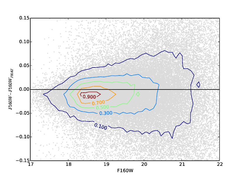
Figure 1: Comparison between our F160W photometry of the published PHAT data and the published PHAT photometry catalogs (Brick 01, Field 09). For this comparison we use the same DOLPHOT parameters that were used in the PHAT catalog. The distribution of the points is illustrated with contour lines of the two-dimensional histogram. The lines show the contours where the histogram falls to 90, 70, 50, 30 and 10 percent of the peak density. The small difference is due to the fact that we use the Anderson PSFs that take into account the spatial variation over the field of view. The median difference between the standard DOLPHOT PSF and the Anderson PSF is $-0.015$ mag which is also the offset we see in the comparison shown here.

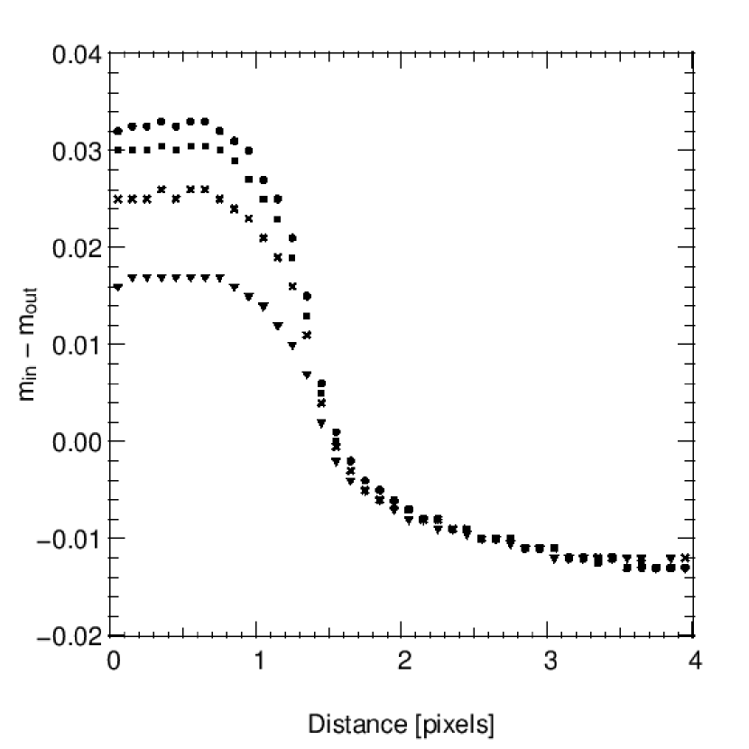
Figure 2: Impact of crowding on our Cepheid sample depending on the distance of the closest source. For each Cepheid a fake source with the same magnitude as the Cepheid is put in the proximity of the Cepheid. This is done iteratively 10000 times for each Cepheid. The difference in magnitude of the fake source ($m_{\mathrm{in}}$) and the recovered source ($m_{\mathrm{out}}$) is a measure of the impact of the Cepheids environment on the crowding. This median difference for all iterations of all Cepheids is shown for different distance bins of the closest source to the fake source. $m_{\mathrm{in}}-m_{\mathrm{out}}$ should be zero for large distances, but due to the background determination it is $\approx-0.01~{}\mathrm{mag}$. This behavior gets worse if the standard background determination parameter is used instead of the parameter for highly crowded fields that is used here. Crowding is only relevant for sources that have the closest source closer than 1.5 pixels. For separations closer than 1 pixel the pixel quantization causes a plateau. Even then the magnitude typically changes only by $0.035~{}\mathrm{mag}$. For these very close separations DOLPHOT might not recover the fake source, which means that there is blending (which is not examined here). The crowding does also depend on the magnitude difference between the fake source and the closest source. The triangles show the crowding for magnitude differences of $3$ mag or larger (i.e. the fake source is at least $3$ mag brighter that the closest source), the crosses for $2$ mag or larger, the squares for $1$ mag or larger and the points for all magnitude differences (including the cases where the fake source is fainter than the closest source).

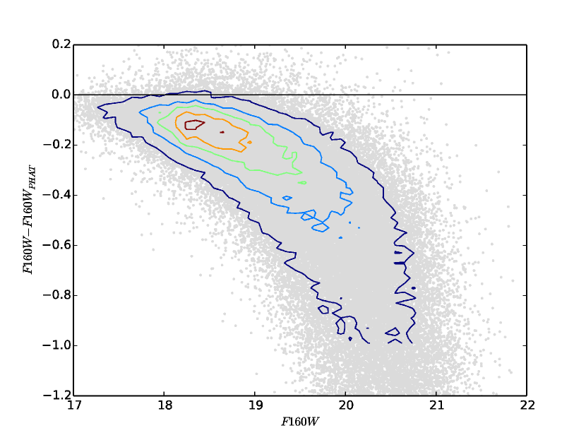
Figure 3: Same as Fig. 1 but with a DOLPHOT sky fitting parameter that is recommended for highly crowded fields. Due to the change in the background determination method our photometry is not consistent any more to the published PHAT catalog. The sky fitting affects the faint stars more than the bright stars. This trend might affect the slope of the PLR but indeed the photometry of the Cepheids only changes slightly due to their brightness. The results are not significantly affected by the change in sky fitting parameter.

We developed a pipeline that identifies the Cepheids from the first year of PAndromeda observations (K13) in the PHAT data. For each Cepheid the pipeline astrometrically matches the corresponding PHAT frames (of all filters) to the PS1 reference frame. After that step we create stamp outs (i.e. small images around the Cepheid) from the aligned PHAT data and the PS1 data. Additionally the pipeline produces difference images from the PHAT data. The number of epochs for each Cepheid is highly dependent on its position (i.e. if it is in an overlap of PHAT bricks). However, due to the observing strategy the optical PHAT filters have at least two epochs (c.f. Fig. 5 in Dalcanton et al. (2012)). Then the Cepheid is identified automatically from these PHAT difference images. This rather sophisticated procedure is necessary due to the fact that it is often unclear which source is the Cepheid in question, as the HST images resolve the error circle of the PS1 source into typically multiple sources. To make sure that the correct source is selected we inspect the result from the pipeline by eye. This involves checking the PHAT stamp outs and difference frame stamp outs of each Cepheid for consistency. This means making sure that the same source is selected in all filters. The pipeline works remarkably well and the few times it fails the information from the WFC3-UVIS frames helps to identify the correct source visually. R12 use the UVIS information to select the correct source when there is a close neighboring source. Although the UVIS data can be very helpful, the problem with this approach is that there are not always UVIS observations available and that the UVIS data can be too shallow to find the source. This is why a source identification based solely on the UVIS information proved to be inferior to the difference image method.

We were able to identify 557 Cepheids from the 2009 Cepheids published in K13 in the PHAT data (all bands). 528 have F110W (close to J band) measurements and 494 have F160W (H band) measurements. 492 Cepheids have F110W and F160W data. While we use all bands for the source identification, in this paper we will only discuss the Cepheids with WFC3-IR data. The obtained magnitudes are random phased. We perform no phase correction since the PS1 epochs in K13 do not cover all PHAT epochs. The precision of the periods from just the first year of PAndromeda observations can be insufficient to determine the correct phase for some PHAT epochs two years apart from the K13 data. With the full PS1 data set of three years we will be able to perform phase corrections. In the few cases in which multiple PHAT measurements are available we therefore use the mean magnitude.

To check our photometry we compare it to R12. 51 of the 68 R12 Cepheids are contained in the K13 sample. Cepheid vn.2.2.463 is present twice in the R12 sample with the same identifier, position, period and F160W photometry, but with a different F110W photometry. So there are rather 50 of the 67 R12 Cepheids contained in K13. We run the remaining 17 Cepheids through our pipeline and include them in our comparison. We compare the stamp outs provided in R12 to our source identification and find only one deviation. For Cepheid vn.2.3.69 (PSO J011.4455+41.9120) our difference frames indicate that the variable source (Cepheid) is indeed the source next to the one identified in the R12 stamp out. We marked this Cepheid with a red D in Fig. 4 and Fig. 5. Fig. 4 shows a mean magnitude difference in F160W photometry of $-0.019\pm 0.011$ mag. Fig. 5 indicates a mean magnitude difference of $-0.258\pm 0.010$ mag in F110W. The two outliers below $\Delta m<-0.5$ mag have a very close source nearby and the offset can be explained by the fact that R12 use aperture photometry in F110W. However that does not explain the offset of approximately a quarter of a magnitude in F110W. This difference remains approximately the same if we perform aperture photometry. The reason for this offset is that R12 used the STScI table for the aperture correction that gives the ensquared energy fraction vs. the aperture size in pixels but assumed this to be the encircled energy fraction (A. Riess, private communication 2014). This explains the offset in F110W. We conclude that our photometry matches that of R12.

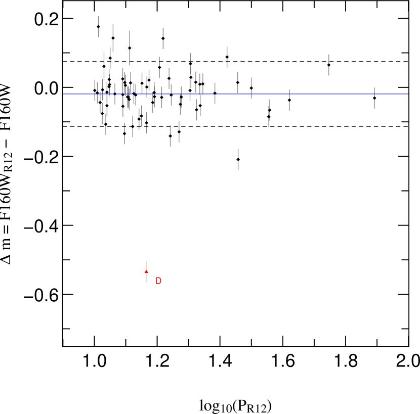
Figure 4: Comparison of our photometry with R12. The Cepheid marked in red (inverted triangle) with a D is due to a misidentification in R12. The mean magnitude difference is $\Delta m=-0.019\pm 0.011$ mag (blue solid line). The standard deviation is shown as a black dashed line.

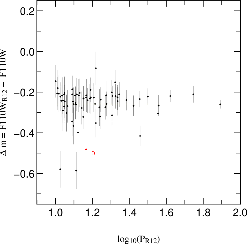
Figure 5: Same as Fig. 4 but with a mean $\Delta m=-0.258\pm 0.010$ mag. The two outliers with $\Delta m<-0.5$ mag are likely due to a close second source that contaminates the aperture photometry of R12. We reproduce the large difference in photometry when performing aperture photometry ourselves. The offset can be explained by an error in the aperture correction in R12.

3 Outlier rejection

After finding 492 Cepheids with F110W and F160W photometry in the PHAT data we want to investigate the Period-Luminosity relation (PLR). As a first step we have to exclude the outliers of our sample that can be seen in Fig. 6. The Wesenheit magnitude, which is reddening-free, used in this figure is defined as:

$$W=m_{F110W}-R\cdot(m_{F110W}-m_{F160W})$$ (1)

where $R$ can be obtained from Schlafly & Finkbeiner (2011, table 6 with $R_{V}=3.1$)

$$R=\frac{A_{F110W}}{A_{F110W}-A_{F160W}}=2.39$$ (2)

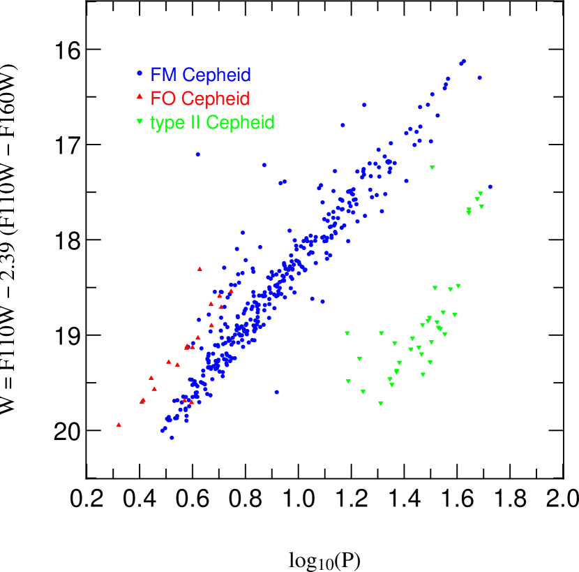
Figure 6: Unclipped Wesenheit Period-Luminosity diagram of 413 classified Cepheids. The shown classification is from K13. The unclassified Cepheids are omitted. The diagram shows the necessity of outlier rejection. The different reasons for outliers as well as an outlier rejection procedure are discussed in Section 3.

There are different reasons for outliers in the period-luminosity relation, namely blending, crowding, extinction, misidentification and misclassification. In the case of blending multiple sources sit along the same line of sight. This is the most difficult case to resolve due to the fact that it needs extensive modeling to do so. Vilardell et al. (2007) studied the impact of blending on the M31 distance and concluded that blending impacts the M31 distance on a $\sim 0.1$ mag level which makes it as significant as the impact of metallicity. Crowding introduces errors in the photometry due to overlapping point spread functions (PSFs). This is obviously worse in ground based observations where the PSFs are larger. The Hubble space telescope (HST) PSF is well determined and stable and as discussed in the previous section (see Fig. 2), crowding does not significantly contribute to our photometric errors. Determining the correct extinction for each Cepheid with spectroscopy is un practical for Cepheids in M31 due to the long exposure times needed and the large spatial extent of M31. In our case we have NIR photometry available for which the extinction is low (McGonegal et al., 1982). Another way to get a handle on extinction is to use Wesenheit magnitudes $W$ that are independent of reddening.

The simplest cause for an outlier is misidentification, i.e. selecting the wrong source when matching two samples. Due to the method of identifying the PS1 Cepheid in PHAT from difference images this kind of mismatch should not be present in our sample. A misclassification of the Cepheid type (fundamental mode (FM), first overtone (FO) and type II) or the identification of a different kind of variable as a Cepheid can also lead to an outlier in the PLR.

The Cepheid type determined by K13 is biased by blending and crowding. Separating FM and FO Cepheids in M31 using ground-based observations is difficult. Ideally, the type would be determined with near infrared light curves. For larger wavelengths the scatter in the PLR is smaller because the temperature sensitivity on the surface brightness is smaller for longer wavelengths (Madore & Freedman, 2012). Even in HST data a Cepheid that is clearly FO in the F160W PLR scatters into the FM in the F814W PLR. For this reason we exclude all unclassified Cepheids from K13 from our sample. This leaves us with 447 Cepheids in F110W and 415 Cepheids in F160W. 413 Cepheids have photometry in both bands simultaneously.

The typical photometric errors we get from DOLPHOT are 0.003 mag. These are very small and do not account for the dispersion of the PLR. The photometric errors are only one aspect that contributes to the dispersion. Extinction and the inherent width of the PLR due to the temperature dependence of the instability strip (Sandage, 1958) are other aspects. In the case of the Wesenheit PLR, different extinction laws for each Cepheid would change $R$ (Equation 2) and therefore increase the scatter in the PLR. The photometric errors in R12 are also very small and as mentioned in E14, Riess et al. (2011) add 0.21 mag in quadrature to the magnitude errors. An ordinary clipping routine without priors or rescaling of the magnitude errors performs very poorly. Introducing priors and rescaling the errors works, but that either usually clips a large fraction of the data or the outlier rejection is unsatisfactory. Testing this method we found no working compromise between clipping away way too much or almost nothing. The problem of outlier clipping and potential implications on the PLR-biases has been recently investigated in detail by E14. As pointed out by E14 that approach possibly underestimates the errors of the PLR. Additionally the combination of priors and strong clipping would prevent a study of the broken slope in our data as was done by Sandage et al. (2009) for their BVI data. On the other hand stricter outlier rejection leads to less blending in the crowded central region of a galaxy (Mager et al., 2013)

We therefore develop a simple outlier rejection method that does not rely on any prior. In the first iteration of the algorithm we assign all measurements the same error and perform a linear fit. The error we assign in the first iteration is the average magnitude error. This ensures (empirically) that at least one Cepheid is above the clipping threshold. After excluding the largest outlier to that fit we calculate the dispersion. For the next step we set the median of the absolute regression residuals (median absolute deviation; MAD) as the magnitude error. After the fit the worst outlier over a threshold of $\kappa$ times the MAD is rejected and the new MAD is calculated. This is repeated until the procedure converges. This is a slightly modified $\kappa$ - $\sigma$ clipping with the MAD for each magnitude error. Another difference to a typical $\kappa$ - $\sigma$ clipping is that only the worst outlier is clipped in one iteration step. A normal $\kappa$ - $\sigma$ clipping without a prior to the slope of the PLR can be heavily influenced by even a few outliers. These outliers could influence the PLR fit in a way that the slope is somewhere between the real PLR and the outliers. The normal $\kappa$ - $\sigma$ clipping would than clip both from the outliers and the real PLR. Clipping only one outlier in one iteration step ensures that an initially wrong PLR fit gradually converges to the genuine PLR and does not clip non outliers on the way. The reason for using the MAD instead of the dispersion is that in this way it is possible to clip Cepheids with a misclassified type, or spurious, or odd (e.g., Polaris-like) Cepheids. (see Fig. 6).

We perform the outlier rejection in the Wesenheit PLR. As a consequence this means that we need both F110W and F160W photometry simultaneously and therefore our sample will consist of 413 Cepheids (FM, FO and type II Cepheids) before the clipping is performed. The main reason for using the Wesenheit function is to minimize the bias caused by extinction and to have a homogenous sample in both F110W and F160W. Clipping in each filter separately could lead to a Cepheid being rejected in one filter but not in the other. Our $\kappa=4$ clipped Wesenheit PLR can be seen in Fig. 7, while the clipped outliers can be seen in Fig. 8.

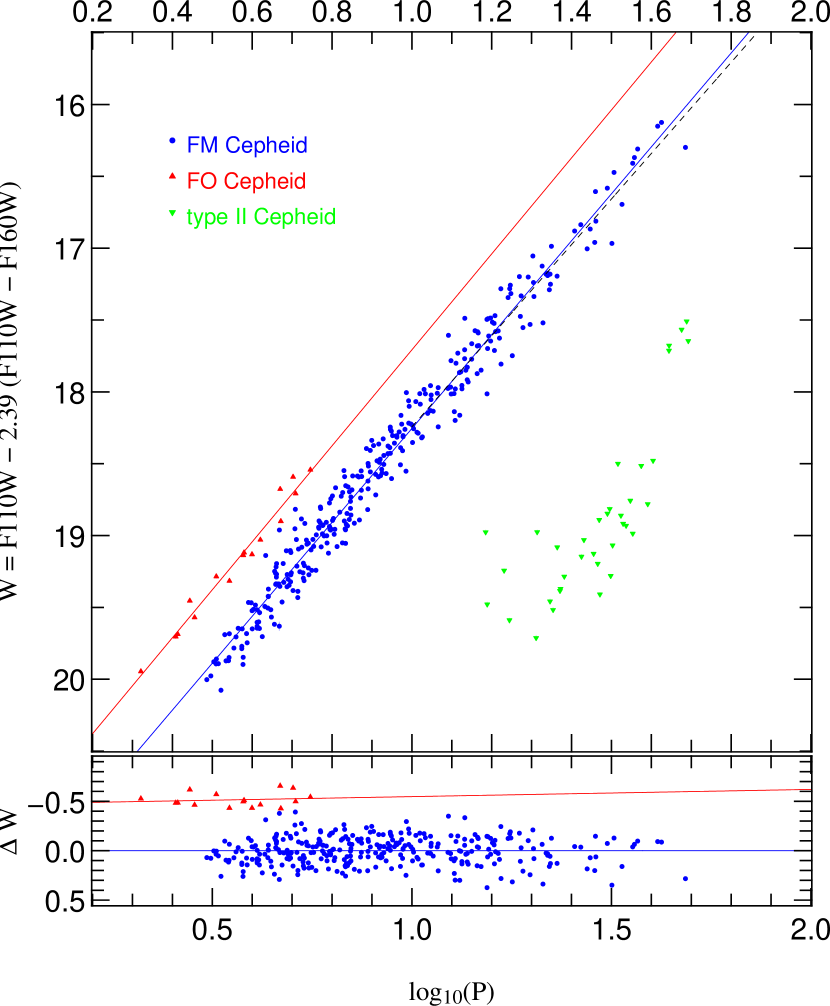
Figure 7: Wesenheit Period-Luminosity relation clipped with the MAD method. The fit parameters to the FM (319 Cepheids, blue solid line) and FO (16 Cepheids, red solid line) PLRs are given in Table 1 ($\#7$ for the FM and $\#9$ for the FO). The 36 type II Cepheids apparently show no linear relationship (see Section 4). The $\log(P)>1$ FM PLR is shown as a black dashed line ($\#8$ in Table 1). The photometric errors (0.009 mag on average) are smaller than the symbols. The bottom panel shows the residuals relative to the FM fit.

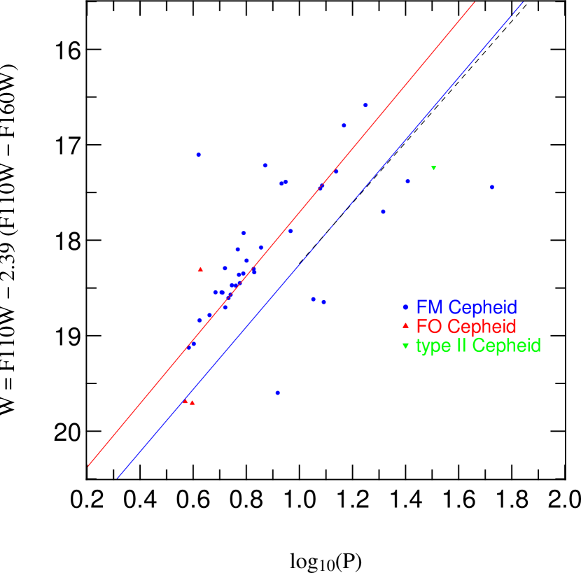
Figure 8: Clipped outliers by the MAD method. The PLR relations are the same as in Fig. 7. Most of the outliers are most likely due to a misclassified Cepheid type.

The number of clipped Cepheids is 42 (38 FM, 3 FO and 1 type II), $\sim$ 10% of the sample. As can be seen most of our outliers are too bright in respect to the best fit PLR, which points to misclassification or blending. About half of the clipped FM Cepheids rejected reside on the FO PLR. Most of the outliers at $0.55\lesssim\log(P)\lesssim 0.85$ are most likely misclassified as FM instead of being classified as FO. Indeed a lot of them are in a region of the amplitude ratio ($A_{21}$) diagram (Fig. 9) populated by both FO and FM Cepheids, which makes them difficult to classify. This is especially true when the light curves, as in our case, are determined from ground based observations in optical bands. Crowding and blending will influence $A_{21}$ which contributes to the misclassification. Blending will decrease amplitudes and the influence of crowding depends on the magnitude difference of the two sources (c.f. Fig. 2). Extinction does not influence the type classification since the classification in K13 only uses the Fourier parameters of first and second order and the extinction only changes the zeroth order (i.e. the mean magnitude). But the greatest contributing factor for the misclassification will be that FO Cepheids populate more than the region characterized in the amplitude ratio diagram in Fig. 9. To resolve this issue we would need spectroscopy or light curves in the near infrared (e.g., see Baranowski et al., 2009). The two clipped sources with the largest periods are also in a transition region between FM and type II in the phase difference diagram (see right panel Fig. 9, K13) and could therefore also be misclassified.

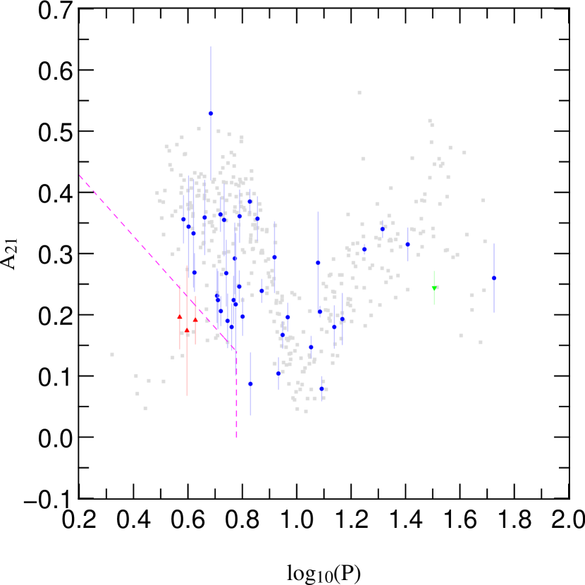
Figure 9: Amplitude ratio diagram. The amplitude ratio $A_{21}$ is determined from a Fourier decomposition in the $r_{P1}$ band (K13). All Cepheids that are not clipped (c.f. Fig. 7) are plotted as gray squares. For better visibility the errors for those Cepheids are omitted. The clipped Cepheids (c.f. Fig. 8) are shown as blue circles (FM), red triangles (FO) and inverted green triangles (type II). The dashed magenta lines define the boundary that was used in K13 to define the parameter space of FO Cepheids. As already discussed in K13 there is a transition region between FM and FO Cepheids and this is most likely the reason that most of the FM outliers that reside on the FO PLR at $\log(P)\sim 0.75$ (c.f. Fig. 8) are misclassified as FM and are rather FO.

E14 introduces an internal scatter $\sigma_{int}$ to the $\chi^{2}$ minimization in order to obtain a $\chi^{2}$ of unity:

$$\chi^{2}=\sum\limits_{i}\frac{(m_{W,i}-m_{W}^{P})^{2}}{(\sigma_{phot,i}^{2}+\sigma_{int}^{2})}$$ (3)

The clipping is performed iteratively until convergence. Fig. 10 shows the clipped Wesenheit PLR if clipped with the E14 method. Fig. 11 shows the corresponding outliers. With a threshold of $\kappa=3$ this algorithm clips 39 FM, 0 FO and 1 T2 Cepheid. For the FM Cepheids the parameters of the fitted line and the dispersion are close to the those of the MAD clipping method (c.f. Table 1). This is not surprising since the sample is the same but for one FM Cepheid that is additionally clipped by the E14 method. Of course the threshold was also chosen such that both methods perform as identically as possible, while still using an integer value for the threshold. If we would not require the threshold to be integer, we could find a threshold that gives the same result as the MAD clipping. Using the same threshold for the FO Cepheids as for the FM Cepheids results in no clipping at all. The MAD method on the other hand does only require one threshold for all Cepheid types. The convergence of the internal scatter method is very sensitive to the threshold $\kappa$ and the starting value of $\sigma_{int}$ (we chose $\sigma_{int}=0$). While the basic idea behind both methods is the same, namely increasing the error by a constant that is described by the dispersion, the method introduced by E14 requires one additional free parameter and according to our tests the convergence performance depends on the starting parameters. The MAD clipping method on the other hand does not depend on the starting parameters and is very easy to implement.

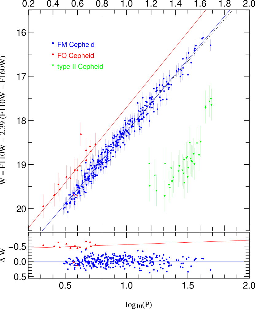
Figure 10: Wesenheit Period-Luminosity relation clipped with the E14 method. The fit parameters to the FM (blue solid line) and FO (red solid line) PLRs are given in Table 1 ($\#10$ for the FM and $\#12$ for the FO). The $\log(P)>1$ FM PLR is shown as a black dashed line ($\#11$ in Table 1). Same as in Fig. 7 the type II Cepheids show no linear relationship (see Section 4). The errors shown here are $\sigma=\sqrt{\sigma_{phot}^{2}+\sigma_{int}^{2}}$, where $\sigma_{phot}$ is the photometric error which is very small compared to the internal scatter $\sigma_{int}$.

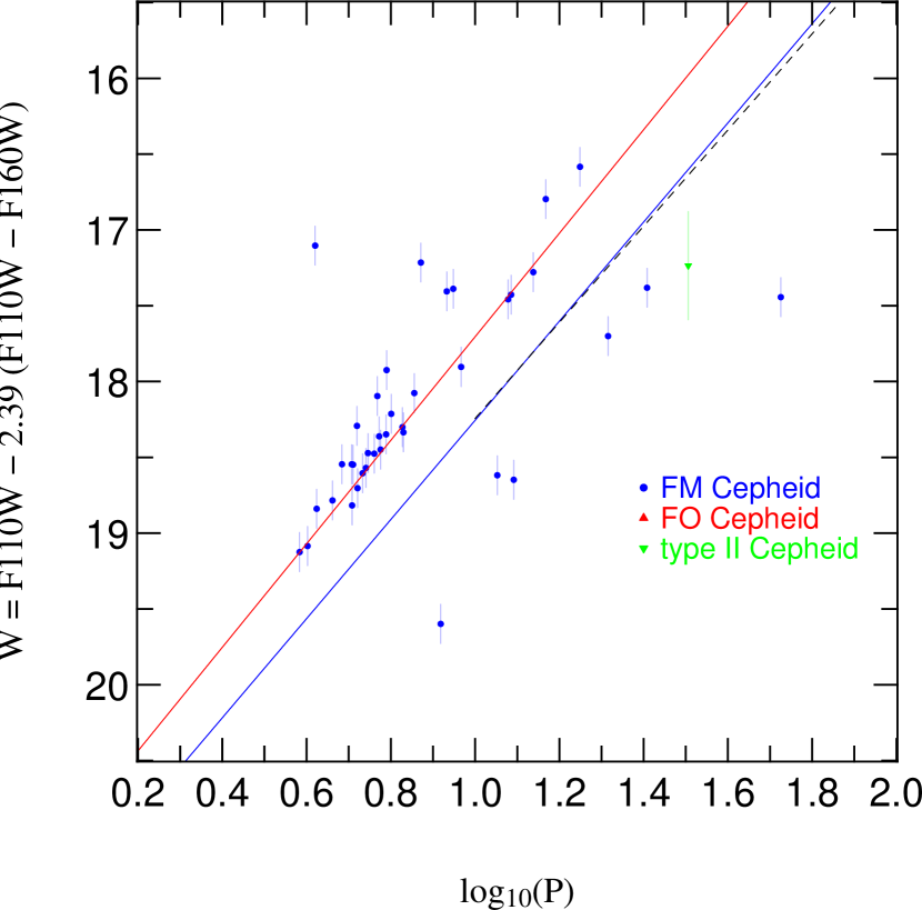
Figure 11: Clipped outliers by the E14 method. The PLR relations are the same as in Fig. 10. None of the FO Cepheids are clipped (3 for the MAD method) and one additional Cepheid is clipped in comparison to the MAD clipping method (c.f. Fig. 8).

4 The adopted Period-Luminosity relations

The F110W and F160W PLRs are shown in Fig. 12 and Fig. 13. Table 1 contains the corresponding best fit parameters. The fits of the Wesenheit PLRs shown in Fig. 7 and Fig. 10 are also included in this table. The PLR fits are of the form $m=a+b\cdot\log(P)$ with a dispersion of $\sigma$. $N_{fit}$ is the number of Cepheids contributing to the fit and $\sigma_{int}$ is given for the cases where the internal scatter clipping method was used (Efstathiou, 2014, see also Equation 3). We included the type II Cepheids in the figures but do not fit a PLR since these do not appear to show one clear linear relationship. Another reason not to fit a PLR is that the transition between W Vir stars and RV Tauri is at $\log(P)\approx 1.3$ and according to Matsunaga et al. (2009) the PLRs of both type II subgroups are not collinear. This can also be seen in the recent study of Ripepi et al. (2015) where the RV Tauri stars are not on the linear PLR of the other type II Cepheids.

The R12 PLRs with $b_{F110W}=-2.725~{}(0.150)$ and $b_{F160W}=-3.003~{}(0.127)$ are steeper than our corresponding slopes (the slopes for the $\log(P)>1$ subsample: $\#2$ and $\#5$ in Table 1). The Wesenheit slope cannot be compared since R12 use $R=1.54$ while we use a different value (c.f. Equations 1 and 2) derived from Schlafly & Finkbeiner (2011, table 6 with $R_{V}=3.1$). In fact the slopes of the R12 sample are closer to our PLRs for the full sample ($\#1$ and $\#4$ in Table 1). Nevertheless the slopes of both samples agree within their $1\sigma$ error bars.

The R12 PLR fits (Table 2 in R12) are slightly inconsistent to the PLR Fig. 2 given in R12. Reanalyzing the R12 F160W data (with the double entry of Cepheid vn.2.2.463 in the data as mentioned before) we can reproduce the R12 slope but get an offset of 0.06 mag for $m(\log(P)=1.2)$. This PLR is closer to the one shown in the R12 PLR plot.

The comparison of the slopes can also be seen in Fig. 14. The theoretical predictions of Bono et al. (2010) for the slopes of the different subsamples are all steeper than our measurements or those of R12. Unfortunately we cannot compare our results for the Wesenheit PLR with E14 since they use a Wesenheit function that includes V and I band magnitudes, which we do not have.

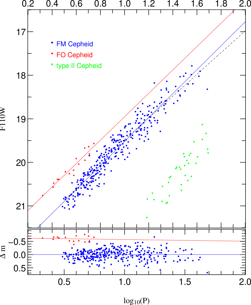
Figure 12: F110W Period-Luminosity relation. The outlier rejection was performed with the MAD method in the Wesenheit PLR (Fig. 7). A Cepheid that was clipped in the Wesenheit PLR was rejected in the near-infrared bands. The fit parameters to the FM (blue solid line) and FO (red solid line) PLRs are given in Table 1 ($\#1$ for the FM and $\#3$ for the FO). The $\log(P)>1$ FM PLR is shown as a black dashed line ($\#2$ in Table 1). The type II Cepheids show no linear relationship (see Section 4)

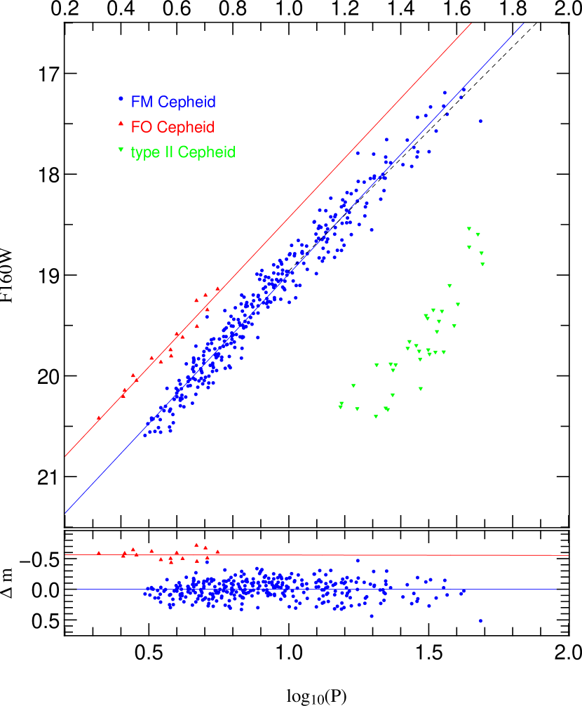
Figure 13: F160W Period-Luminosity relation. The outlier rejection was performed with the MAD method in the Wesenheit PLR (Fig. 7). A Cepheid that was clipped in the Wesenheit PLR was rejected in the near-infrared bands. The fit parameters to the FM (blue solid line) and FO (red solid line) PLRs are given in Table 1 ($\#4$ for the FM and $\#6$ for the FO). The $\log(P)>1$ FM PLR is shown as a black dashed line ($\#5$ in Table 1). The type II Cepheids show no linear relationship (see Section 4)

Table 1: PLR fit parameters

$\#$	band	type	range	$N_{fit}$	a (log P = 1)	slope b	$\sigma$	$\sigma_{int}$	$\chi_{d.o.f.}^{2}$
1	F110W	FM	all	319	19.521 ( 0.012)	-2.749 ( 0.057)	0.204	-	1.000
2	F110W	FM	log P $>$ 1	110	19.476 ( 0.037)	-2.497 ( 0.209)	0.243	-	1.415
3	F110W	FO	all	16	18.953 ( 0.051)	-2.686 ( 0.157)	0.105	-	1.000
4	F160W	FM	all	319	18.991 ( 0.003)	-2.966 ( 0.033)	0.155	-	1.000
5	F160W	FM	log P $>$ 1	110	18.960 ( 0.028)	-2.779 ( 0.171)	0.178	-	1.318
6	F160W	FO	all	16	18.431 ( 0.051)	-2.960 ( 0.145)	0.082	-	1.000
7	Wesenheit	FM	all	319	18.255 ( 0.007)	-3.267 ( 0.071)	0.138	-	1.000
8	Wesenheit	FM	log P $>$ 1	110	18.244 ( 0.016)	-3.172 ( 0.117)	0.147	-	1.145
9	Wesenheit	FO	all	16	17.708 ( 0.134)	-3.339 ( 0.281)	0.074	-	1.000
10	Wesenheit	FM	all	318	18.256 ( 0.004)	-3.270 ( 0.036)	0.136	0.128	1.126
11	Wesenheit	FM	log P $>$ 1	110	18.244 ( 0.016)	-3.172 ( 0.117)	0.147	0.128	1.183
12	Wesenheit	FO	all	19	17.705 ( 0.135)	-3.414 ( 0.282)	0.265	0.265	1.062

Note. — The magnitude errors were set to the same value, namely to the dispersion $\sigma$. In the cases where the E14 clipping method was used ($\#10$, $\#11$ and $\#12$) the internal scatter ($\sigma_{int}$) was added in quadrature to the photometric errors (c.f. Fig. 10). The errors of the fitted parameters were determined with the bootstrapping method. Lines 8 and 11 show identical parameters since the only difference is that the magnitude errors for line 11 include the photometric errors determined by DOLPHOT which as mentioned earlier are negligible compared to $\sigma_{int}$.

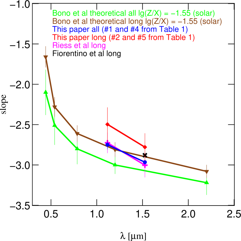
Figure 14: PLR slope dependence on the wavelength. The R12 slopes (magenta) are steeper than our slopes for the long period Cepheid sample ($\log(P)>1$, red, $\#2$ and $\#5$ in Table 1). The Fiorentino et al. (2013) slope with $Z=0.02$ and $Y=0.28$ for long period Cepheids (black) is within the error of the slope of our long period sample result. For a different Helium content the Fiorentino et al. (2013) slope is steeper and would agree with our total Cepheid sample (red, $\#1$ and $\#4$ in Table 1). The theoretical predictions of Bono et al. (2010) are steeper than our measurements for both subsamples.

In the next step we investigate whether our FM Cepheids show any signature of the broken slope proposed by Sandage et al. (2009). For this we use the same approach as in Equations 16 and 17 in K13: We fit two slopes and a common suspension point at 10 days. These fits can be seen in Fig. 15, Fig. 16 and Fig. 17. The fit parameters are summarized in Table 2. All fits show a steeper slope for short period Cepheids ($\log(P)\leq 1$) than for long period Cepheids ($\log(P)>1$) . Note that a Malmquist bias would influence the faint end slope so that it becomes shallower than it actually is. We also perform bootstrapping (resample the data) with 10000 realizations to check how significant the broken slope is and show the results in Fig. 18, 19 and 20. Only for the Wesenheit function there are realizations of the bootstrapping where the 3 $\sigma$ contours overlap. The break at exactly 10 days is often adopted in the literature, but there are also studies contesting that value. Klagyivik & Szabados (2009) for example find that the break occurs at 10.47 days. We discuss the break at 10 days here and provide a table for the relevant parameters of other suspension points in the appendix.

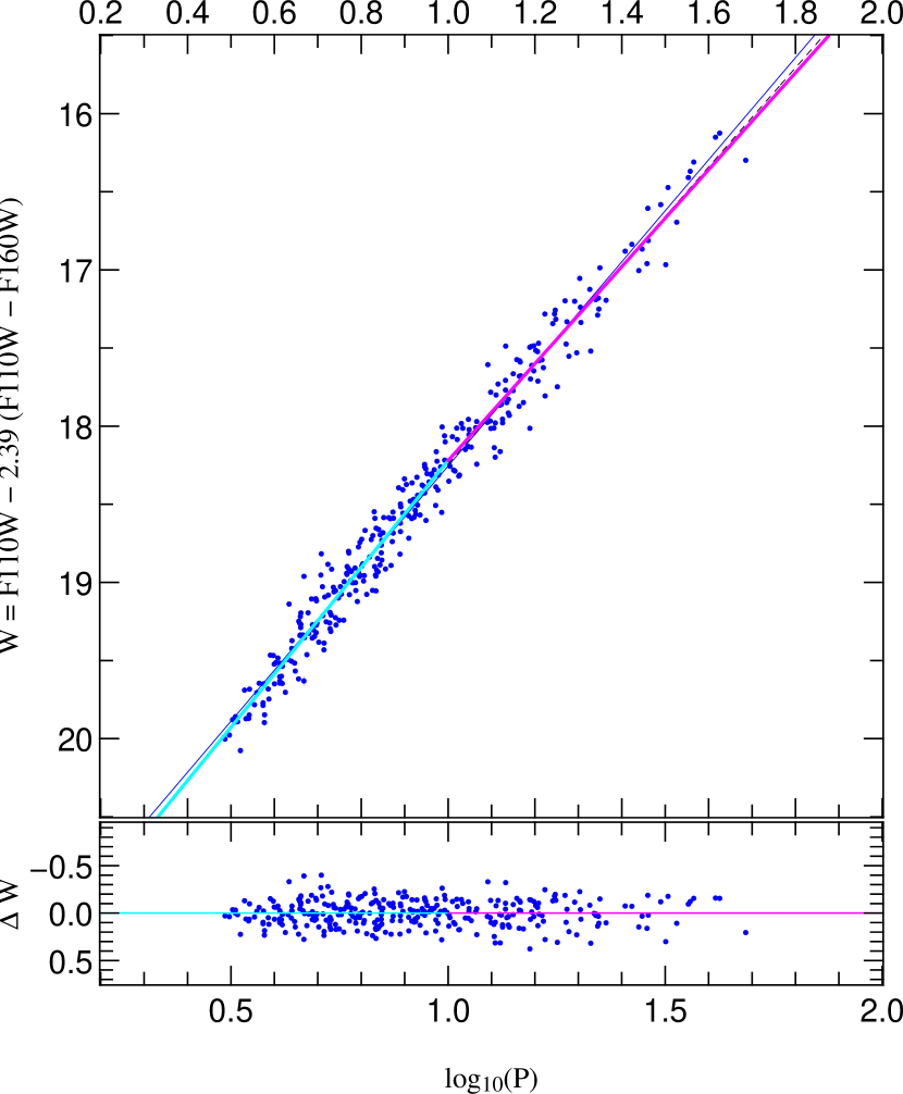
Figure 15: Broken slope Wesenheit PLR for FM Cepheids. A broken slope fit with a common suspension point at 10 days (c.f. Equations 16 and 17 in K13) is shown ($\#1$ in Table 2). The short period Cepheid slope ($\log(P)\leq 1$) is shown in cyan and the long period Cepheid slope ($\log(P)>1$) in magenta. The blue solid line is the linear slope fit ($\#7$ in Table 1) and the black dashed line the fit to the long period Cepheid sample ($\#8$ in Table 1).

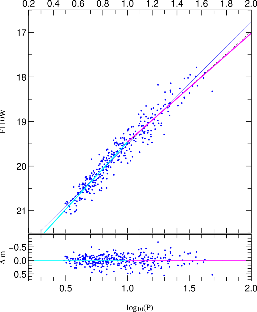
Figure 16: Broken slope F110W PLR for FM Cepheids ($\#2$ in Table 2). Same as Fig. 15 but with $\#1$ (Table 1) as linear slope fit and $\#2$ (Table 1) as fit for the long period Cepheids.

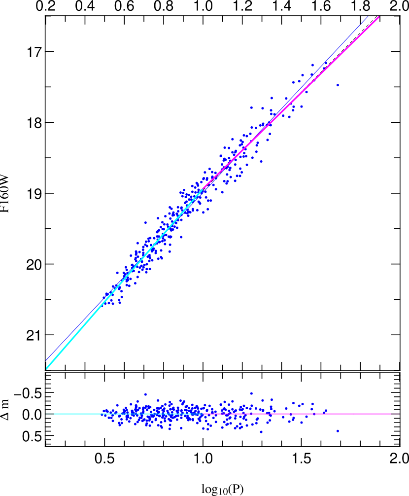
Figure 17: Broken slope F160W PLR for FM Cepheids ($\#3$ in Table 2). Same as Fig. 15 but with $\#4$ (Table 1) as linear slope fit and $\#5$ (Table 1) as fit for the long period Cepheids.

Table 2: broken slope PLR fit parameters

$\#$	band	$b_{\log(P)\leq 1}$	$b_{\log(P)>1}$	$a_{\log(P)=1}$	$\sigma$	$\chi_{d.o.f.}^{2}$
1	Wesenheit	-3.411 ( 0.038)	-3.103 ( 0.060)	18.221 ( 0.013)	0.136	0.978
2	F110W	-3.028 ( 0.078)	-2.433 ( 0.105)	19.455 ( 0.021)	0.200	0.960
3	F160W	-3.188 ( 0.050)	-2.714 ( 0.069)	18.938 ( 0.014)	0.152	0.956

Note. — The magnitude errors were set to the same value, namely to the dispersion $\sigma$ of the corresponding fit in Table 1 ($\#7$, $\#1$ and $\#4$). The errors of the parameters were determined with bootstrapping.

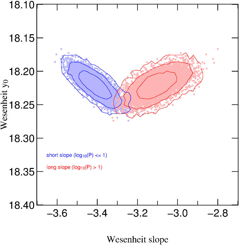
Figure 18: Bootstrapping of the broken slope in the Wesenheit PLR. The common suspension point $y_{0}$ is plotted versus the slope. The short period Cepheid slope ($\log(P)\leq 1$) is shown in blue and the long period Cepheid slope in red. The 1$\sigma$, 2$\sigma$ and 3$\sigma$ contour lines are also shown as solid lines.

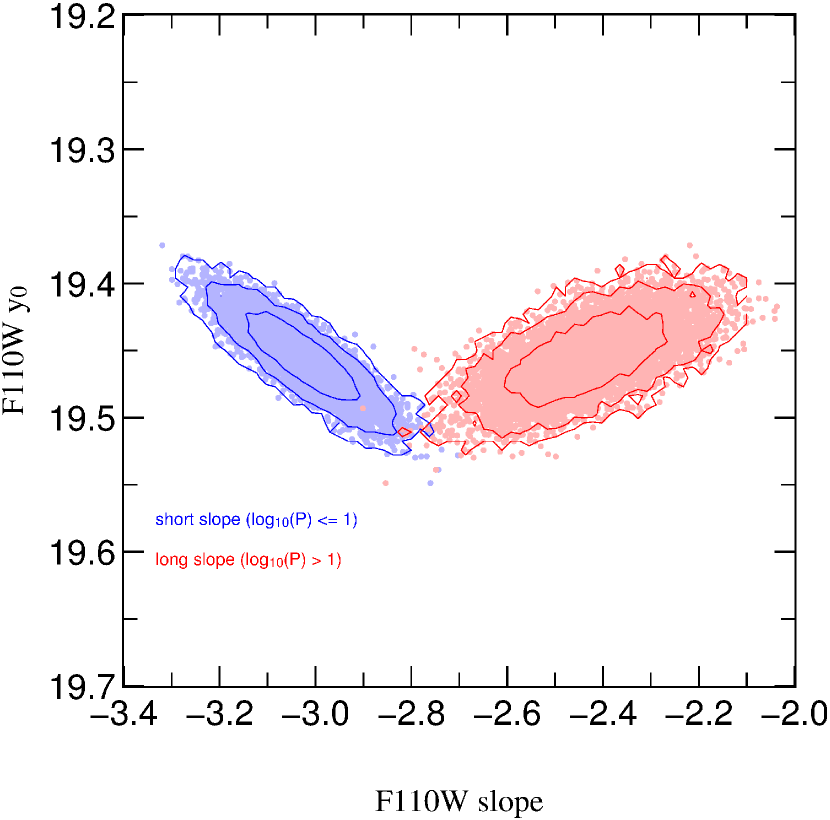
Figure 19: Bootstrapping of the broken slope in the F110W PLR. The legend is otherwise similar to that displayed in Fig. 18.

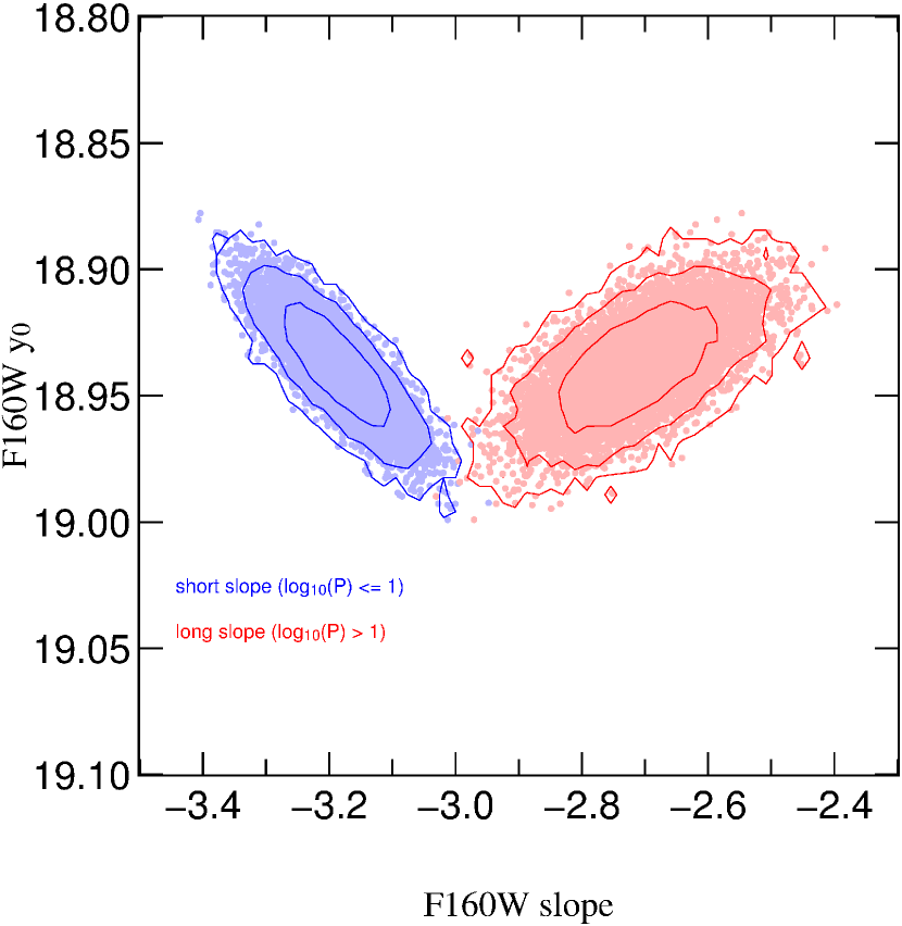
Figure 20: Bootstrapping of the broken slope in the F160W PLR. The legend is otherwise similar to that displayed in Fig. 18.

The results from the bootstrapping already point toward a broken slope. To determine if the broken slope is significantly better than the linear slope we perform an F-test. The advantage of the F-test is that it is not sensitive to the problem of the uncertainty in the adopted magnitude errors. Due to the fact that we chose the magnitude errors to be equal to the dispersion in the linear fit, we are able to get better estimates on the errors of the fitted parameters. However, this approach does not allow us to perform a $\chi^{2}$ test. Following Equations 3.40 and 3.41 from Chatterjee & Hadi (2013) where model 1 is the reduced model with $p_{1}$ parameters and model 2 the full model with $p_{2}$ parameters, the observed F-ratio is:

$$F_{obs}=\frac{[\chi_{1}^{2}-\chi_{2}^{2}]/[p_{2}-p_{1}]}{\chi_{2}^{2}/[N-p_{2}]}$$ (4)

$N$ denotes the number of data points and the $\chi_{i}^{2}$ are the corresponding $\chi^{2}$ of the two models. The critical F-value is

$$F_{crit}=F(p_{2}-p_{1},N-p_{2};\alpha)$$ (5)

for a significance level of $\alpha$, where F is the distribution function of the F-test. For $F_{obs}\geq F_{crit}$ the null hypothesis (that model 2 is not significantly better than model 1) is rejected. Simply put for $F_{obs}\geq F_{crit}$ model 2 is more significant than model 1. In our case model 1 is the linear fit (Table 1) and model 2 the fit with the broken slope (Table 2). For a typical significance level of $\alpha=0.05$ the critical F-value is $F_{crit}=F(1,316;0.05)=3.87$. Our observed F-values are $F_{obs,Wesenheit}=8.24$, $F_{obs,F110W}=14.12$ and $F_{obs,F160W}=15.71$. Therefore all three broken slope fits are significant at a level of at least $1-\alpha=0.95$. We confirm the result from the bootstrapping i.e. the Wesenheit broken slope is less significant than the F110W and F160W broken slopes. Indeed the F110W and F160W broken slopes are also still significant at a 3 $\sigma$ level.

In the next step we check how well the data are described by a parabola instead of a broken linear relation. The parabolic fits are shown in Fig. 21, 22 and 23. The fit parameters are summarized in Table 3. As can already be seen from the $\sigma_{d.o.f.}$ the parabolic fit will practically be as significant as the broken slope.

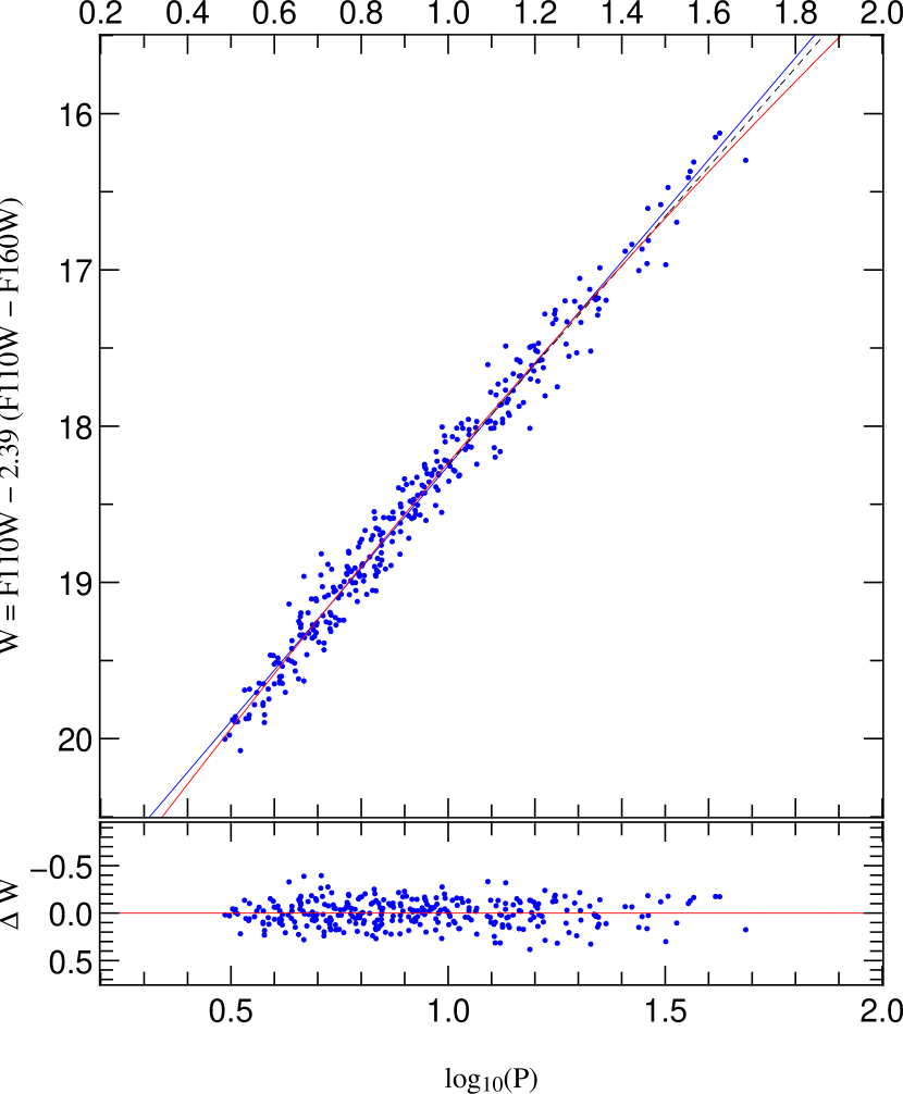
Figure 21: Parabolic Wesenheit PLR for FM Cepheids ($\#1$ in Table 3). The parabola is shown as a red solid line. The blue solid line is the linear slope fit ($\#7$ in Table 1) and the black dashed line the fit to the long period Cepheid sample ($\#8$ in Table 1).

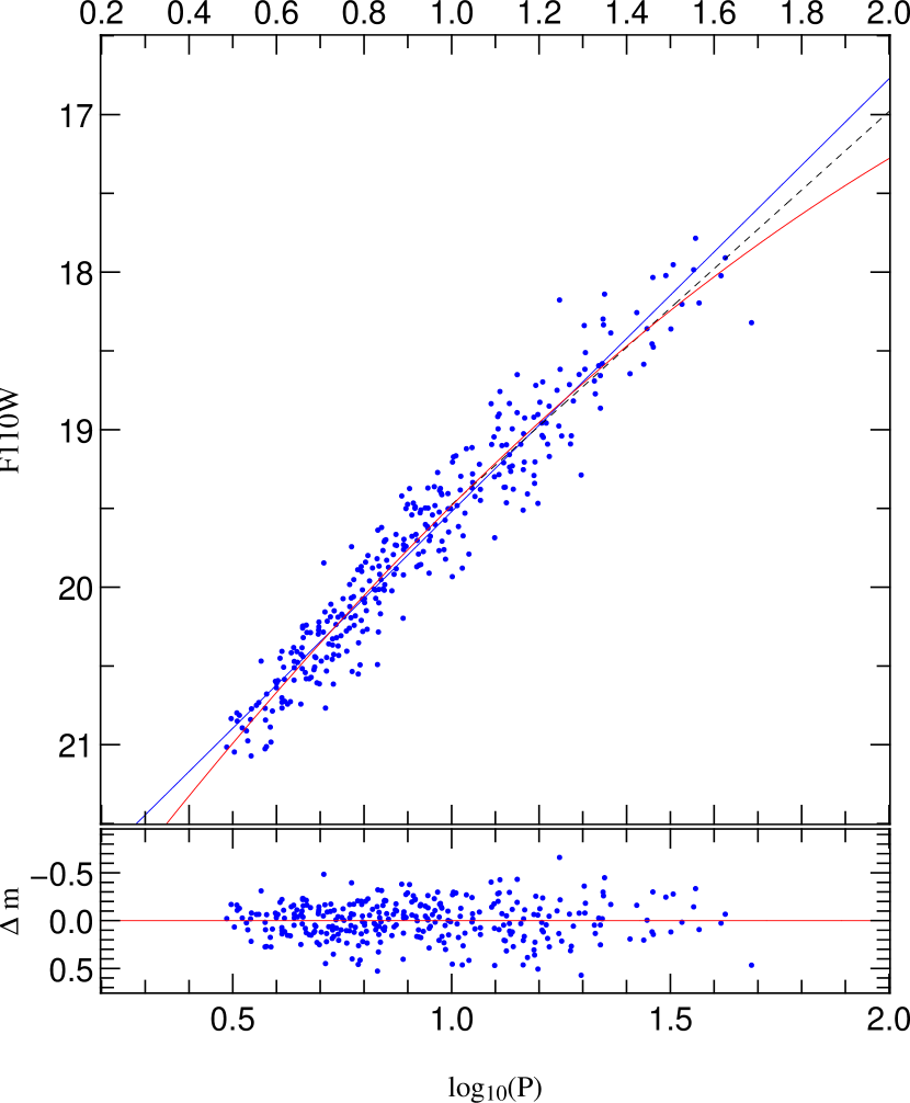
Figure 22: Parabolic F110W PLR for FM Cepheids (red solid line, $\#2$ in Table 3). The blue solid line is the linear slope fit ($\#1$ in Table 1) and the black dashed line the fit to the long period Cepheid sample ($\#2$ in Table 1).

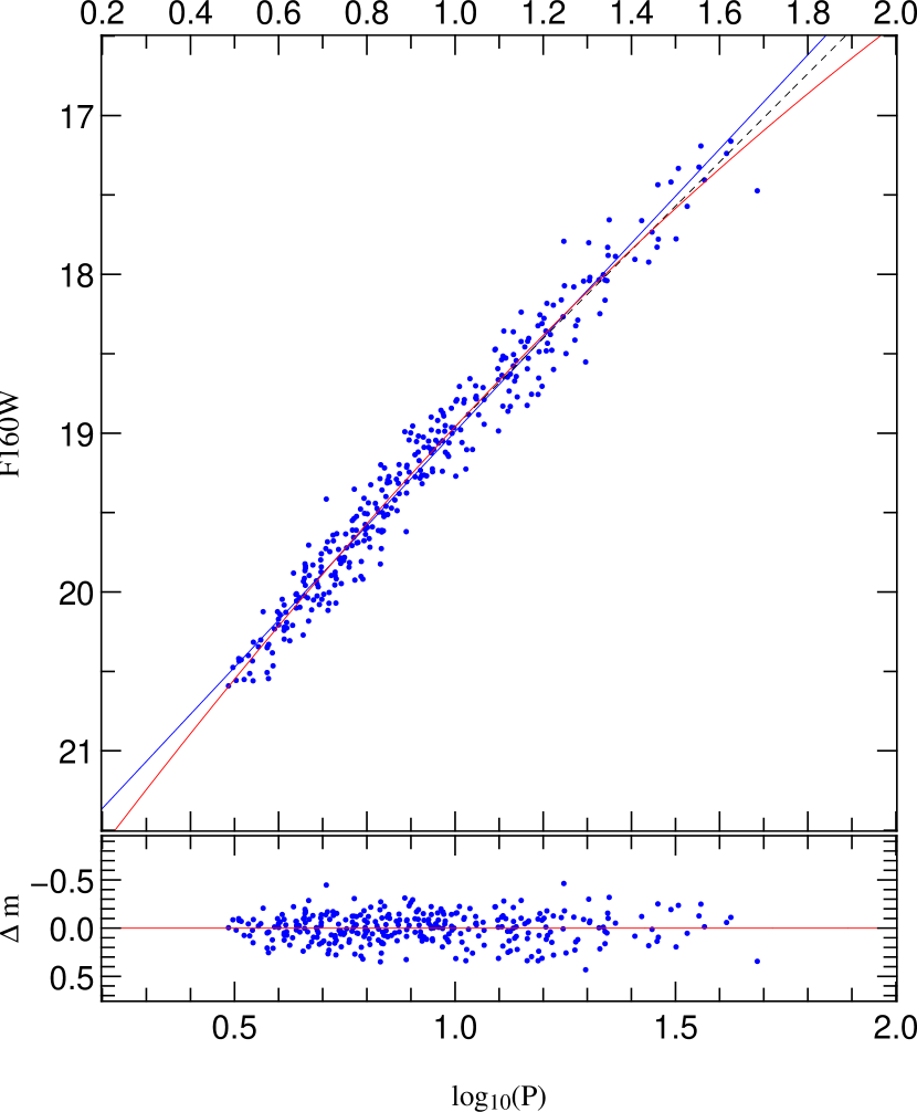
Figure 23: Parabolic F160W PLR for FM Cepheids (red solid line, $\#3$ in Table 3). The blue solid line is the linear slope fit ($\#4$ in Table 1) and the black dashed line the fit to the long period Cepheid sample ($\#5$ in Table 1).

Table 3: parabola PLR fit parameters

$\#$	band	$a_{\log(P)=1}$	$b$	$c$	$\sigma$	$\chi_{d.o.f.}^{2}$
1	Wesenheit	18.236 ( 0.011)	-3.265 ( 0.029)	0.267 ( 0.089)	0.136	0.980
2	F110W	19.482 ( 0.016)	-2.746 ( 0.039)	0.543 ( 0.141)	0.200	0.960
3	F160W	18.960 ( 0.012)	-2.964 ( 0.032)	0.427 ( 0.107)	0.152	0.957

Note. — The magnitude errors were set to the same value, namely to the dispersion $\sigma$ of the corresponding fit in Table 1 ($\#7$, $\#1$ and $\#4$) and the errors of the fit parameters determined with bootstraping. The parabola fit has the form $m=a+b\cdot\log(P)+c\cdot[\log(P)]^{2}$.

A possible reason for the broken slope could be the Hertzsprung progression. With increasing periods the bump in the light curve moves to the maximum (brightest magnitude) of the light curve. For periods larger than 10 days the bump moves away from the maximum (see e.g. K13). Randomly phased observations might be biased toward brighter magnitudes due to the bump in the light curve. This effect would be strongest for Cepheids around 10 days and for larger periods it would decrease again. This would mean that the magnitudes at 10 days are systematically brighter than they should be, which could explain the broken slope.

In the light curves published in Persson et al. (2004) we see that the bumps are stronger in the J band than in the H band. This fits to our result that in the F110W band (close to the J band) the curvature of the parabolic fit to the PLR is stronger than in the F160W band (close to H band). Also the decrease of the slope of the long-period Cepheid PLR as compared to the linear fit to the full sample is stronger in F110W than in F160W. In view of this, an overestimation of the mean magnitudes of Cepheids near $\log(P)=1$ from random-phase data due to the bump presence seems indeed to be a plausible explanation for the observed non-linearity in the PLRs or at least is contributing to this effect. With the full PAndromeda data set of three years we will be able to perform a phase correction and therefore be capable to test whether such a hypothetical bias exists.

5 Implications of the improved PLR on the Hubble constant

As can be seen in Fig. 14 and e.g. in $\#5$ in Table 1 our PLR is different from the R12 PLR. Therefore we want to explore what impact our new sample has on the estimate of the Hubble constant $H_{0}$.

We use method $\#10$ table 3 in R12 where M31 is used as the anchor for the comparison. If we were to use a different fit where M31 only contributes to the fit of the slope, we would have to do the complete analysis of the SN Ia data. So the idea is to only check for relative changes in the anchor and assume nothing changes in the SN Ia galaxy analysis, i.e. plug our sample in as an anchor and leave everything else the same. Furthermore we have to make the reasonable assumption that the photometric offsets between our sample and the R12 sample are well understood and described by:

$$<\Delta m_{\mathrm{F160W}}>=<m_{\mathrm{F160W,R12}}-m_{\mathrm{F160W,K14}}>=-0.019~{}\mathrm{mag}$$ (6)

$$<\Delta m_{\mathrm{F110W}}>=<m_{\mathrm{F110W,R12}}-m_{\mathrm{F110W,K14}}>=-0.258~{}\mathrm{mag}$$ (7)

We have to make this assumption so that we can later compare the offsets between the two samples.

The first step is to fit the color corrected Wesenheit function of the R12 sample with a slope of -3.20 as given by $\#10$ Table 3 in R12 in order to obtain $m(\log(P)=1.2)_{\mathrm{R12}}$. Fig. 24 shows the fit to the color corrected Wesenheit function. In the next step we check how well the color correction factor of $X=-0.066~{}\mathrm{mag}$ in R12 applies to our data. As can be seen in Fig. 25 the color correction factor is also consistent with our sample (the mean offset is only $0.004~{}\mathrm{mag}$) when we apply the offsets described in Equations 6 and 7. The last step is to fit the color corrected Wesenheit function with the offsets in order to obtain $m(\log(P)=1.2)_{\mathrm{K14}}$. The fit shown in Fig. 26 was done with the same slope that was used in the first step. Due to the small photometric errors in our sample the individual data points were not weighted by their errors.

The magnitude difference for the two anchor samples is

$$\Delta M=<m(\log(P)=1.2)_{\mathrm{R12}}-m(\log(P)=1.2)_{\mathrm{K14}}>=17.701~{}\mathrm{mag}-17.769~{}\mathrm{mag}=-0.068~{}\mathrm{mag}$$ (8)

This corresponds to

$$\Delta\mu=(m-M)_{\mathrm{R12}}-(m-M)_{\mathrm{K14}}=\Delta m-\Delta M=-\Delta M=0.068~{}\mathrm{mag}$$ (9)

i.e. only the difference in the anchor is relevant, since $\Delta m=0~{}\mathrm{mag}$ due to the first assumption. Since $d_{L}\sim 1/H_{0}$ we get

$$\Delta\mu_{0}=\mu_{\mathrm{0,R12}}-\mu_{\mathrm{0,K14}}=5\log\left(\frac{d_{\mathrm{L,R12}}}{d_{\mathrm{L,K14}}}\right)=5\log\left(\frac{H_{\mathrm{0,K14}}}{H_{\mathrm{0,R12}}}\right)$$ (10)

and therefore

$$H_{\mathrm{0,K14}}=10^{[\Delta\mu_{0}/5]}\cdot H_{\mathrm{0,R12}}=1.032\cdot H_{\mathrm{0,R12}}$$ (11)

So our sample gives a $3.2\%$ increased $H_{0}$ compared to the R12 sample. This is very surprising when considering that the R12 sample is in large part a subset of our sample. Fig. 27 shows the difference in the two samples.

We checked if there is any indication for this difference in the spatial distribution of the two data sets, since our sample covers more of the M31 area. But the subsets are distributed equivalently across M31. It is not the case that one subsample is located in the spiral arms and the other is not. As can be seen in the appendix the crowding tests also support the argument that the spatial distribution is not the reason for the offset, since the offset only changes slightly.

The offset that is described in this section is very worrisome since it begs the question how well we can constrain $H_{0}$ if a larger Cepheid sample that covers more of the galaxy produces a different $H_{0}$.

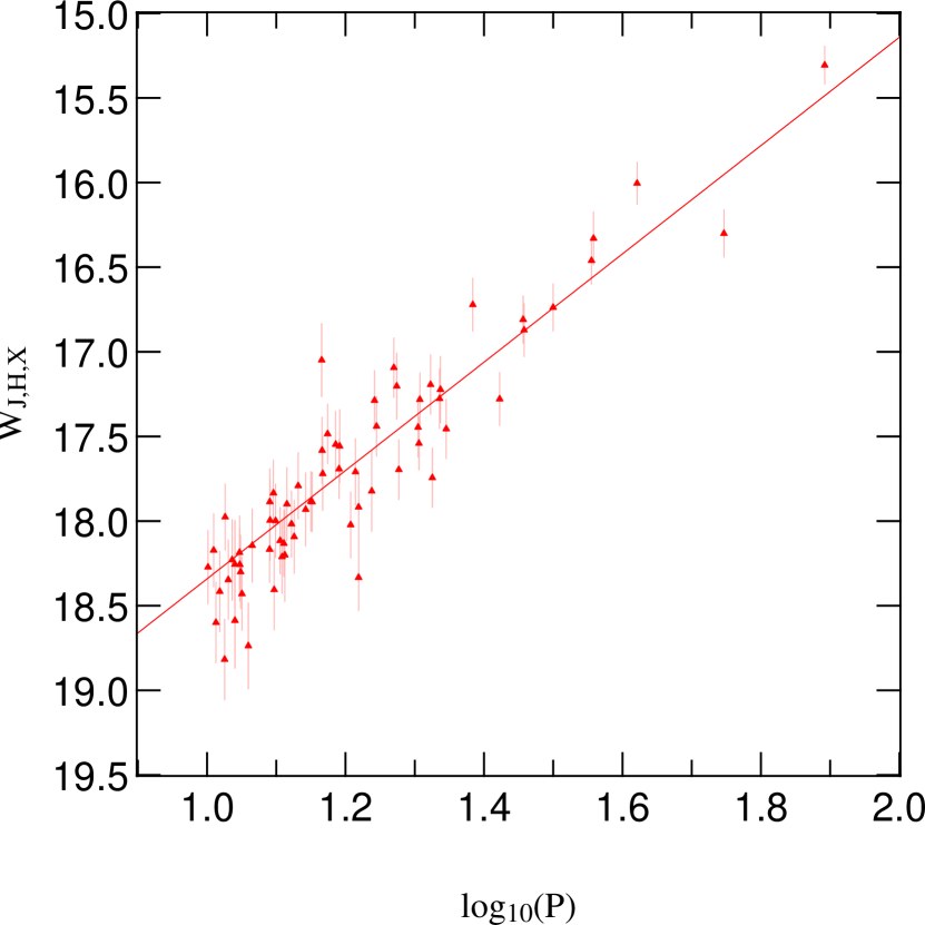
Figure 24: Color corrected Wesenheit ($W_{\mathrm{J,H,X}}=\mathrm{F160W}-1.54(\mathrm{F110W}-\mathrm{F160W}+0.066)$) of the R12 sample. The solid red line shows a fit of the slope of -3.20 ($\#10$ in table 3 R12) to the data. The fit gives a $m(\log(P)=1.2)_{\mathrm{R12}}=17.701~{}\mathrm{mag}$.

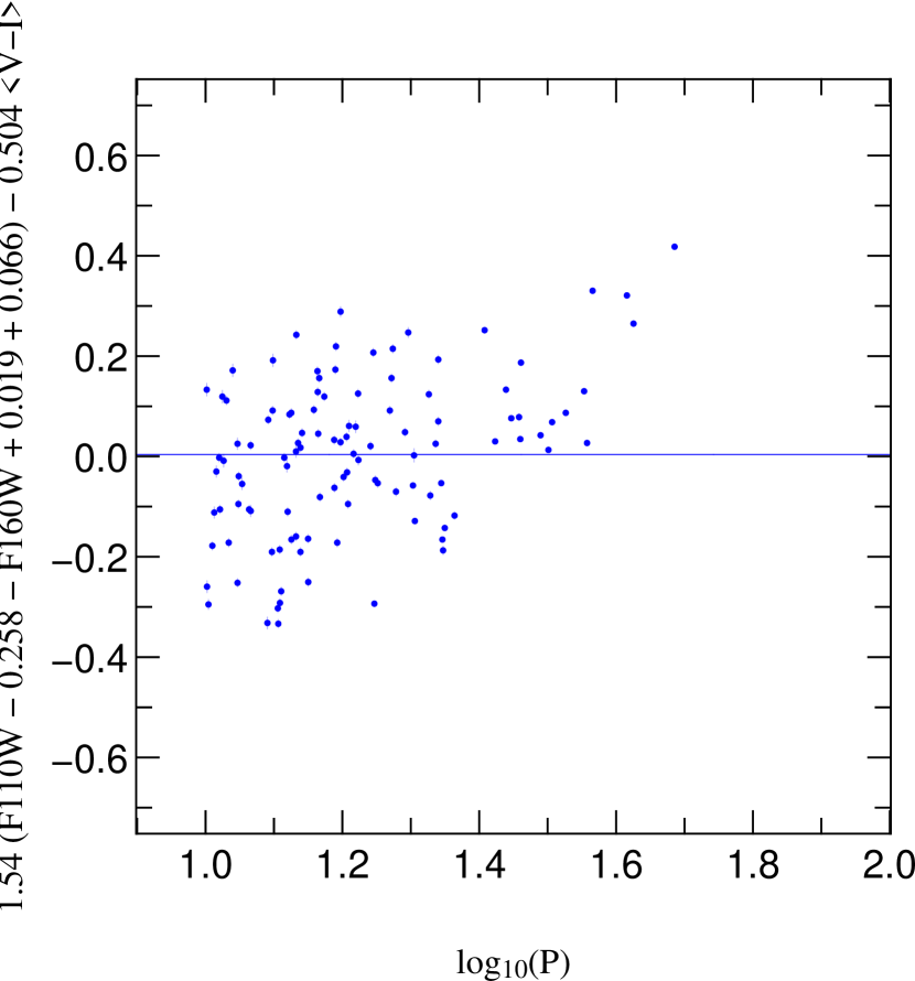
Figure 25: The plot shows how well the color correction factor of $X=-0.066~{}\mathrm{mag}$ from R12 fits to our data that was transformed to the same photometric system used in R12 (i.e. with applied offsets). The blue solid line shows the mean offset of $0.004~{}\mathrm{mag}$. The brightness trend is also present in R12.

Figure 26: Color corrected Wesenheit ($W_{\mathrm{J,H,X}}=\mathrm{F160W}-0.019-1.54(\mathrm{F110W}-0.258-\mathrm{F160W}+0.019+0.066)$) for our sample. Same as in Fig. 24 the solid line shows a fit of the -3.20 slope to the data. The fit gives $m(\log(P)=1.2)_{\mathrm{K14}}=17.769~{}\mathrm{mag}$, which means that our sample is fainter than the R12 sample.

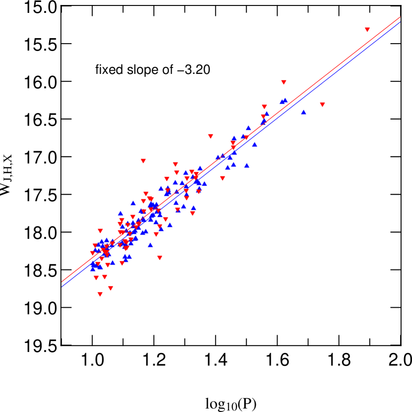
Figure 27: Comparison between Fig. 24 and Fig. 26. The blue triangles are our Cepheids, while the inverted red triangles are the R12 Cepheids. The Wesenheit $W_{\mathrm{J,H,X}}$ is the color corrected Wesenheit function as defined in Fig. 24 and Fig. 26 for the respective samples (i.e. the blue Cepheids have the offsets applied as defined in Equations 6 and 7). Both fits use a fixed slope of -3.20 that was also used in R12 for the SN Ia host galaxies.

6 Conclusion

In this paper we present a new method of outlier rejection that does not rely on priors and is capable of clipping misclassified first overtone (FO) Cepheids from the fundamental mode (FM) Cepheid sample. The method is similar to the outlier rejection method established by E14. Both use the dispersion to correct the underestimated errors from photometry. The difference is that our median absolute deviation clipping method does not use an additional free parameter.

We use the publicly available PHAT (Dalcanton et al., 2012) data to obtain near-infrared photometry of a subsample of Cepheids published in K13. Our data reduction pipeline takes the HST and PS1 difference images into account in order to identify the correct source in the PHAT data. With the MAD clipping method we obtain a sample of 371 Cepheids with F110W and F160W photometry. The sample consists of 319 FM, 16 FO and 36 type II Cepheids. 110 FM Cepheids have periods of 10 days or more. The slopes of our PLRs for Cepheids with periods of 10 or more days are shallower than the slopes obtained by R12, but agree within the $1\sigma$ errors.

We check our sample for a broken slope in the PLR and find that a broken slope describes the data significantly better than a linear slope.

An estimation of the effect of our PLRs on the Hubble constant shows that our sample gives a $3.2\%$ larger $H_{0}$ than the R12 sample.

With the full three years of PAndromeda data the Cepheid sample will increase, especially toward longer periods. Additionally we will be able to perform phase correction to the PHAT data. This will help to distinguish between a broken slope PLR and a parabolic PLR. The phase correction will also improve the dispersion further, resulting in an even tighter constrained PLR.

Appendix A Appendix

Our sample will be published in electronic form on the CDS.

A.1 Stampouts

The stampouts of the 371 Cepheids (319 FM Cepheids, 16 FO Cepheids and 36 type II Cepheids) can be seen in Fig. 28, Fig. 29, Fig. 30 and Fig. 31. The stampouts for the clipped outliers are shown in Fig. 32. The scaling in each stampout is different and calculated automatically. Therefore the brightness between two stampouts cannot be compared. Each stampout has the width of 2.5 arcsec and the white circle centered around the Cepheid has a radius of 0.5 arcsec.

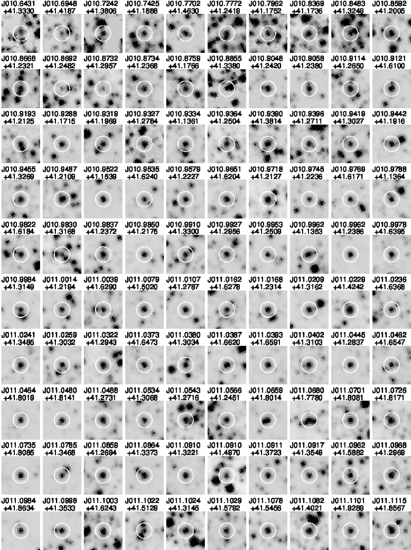
Figure 28: Cepheid stampouts

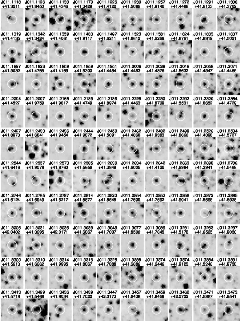
Figure 29: Cepheid stampouts

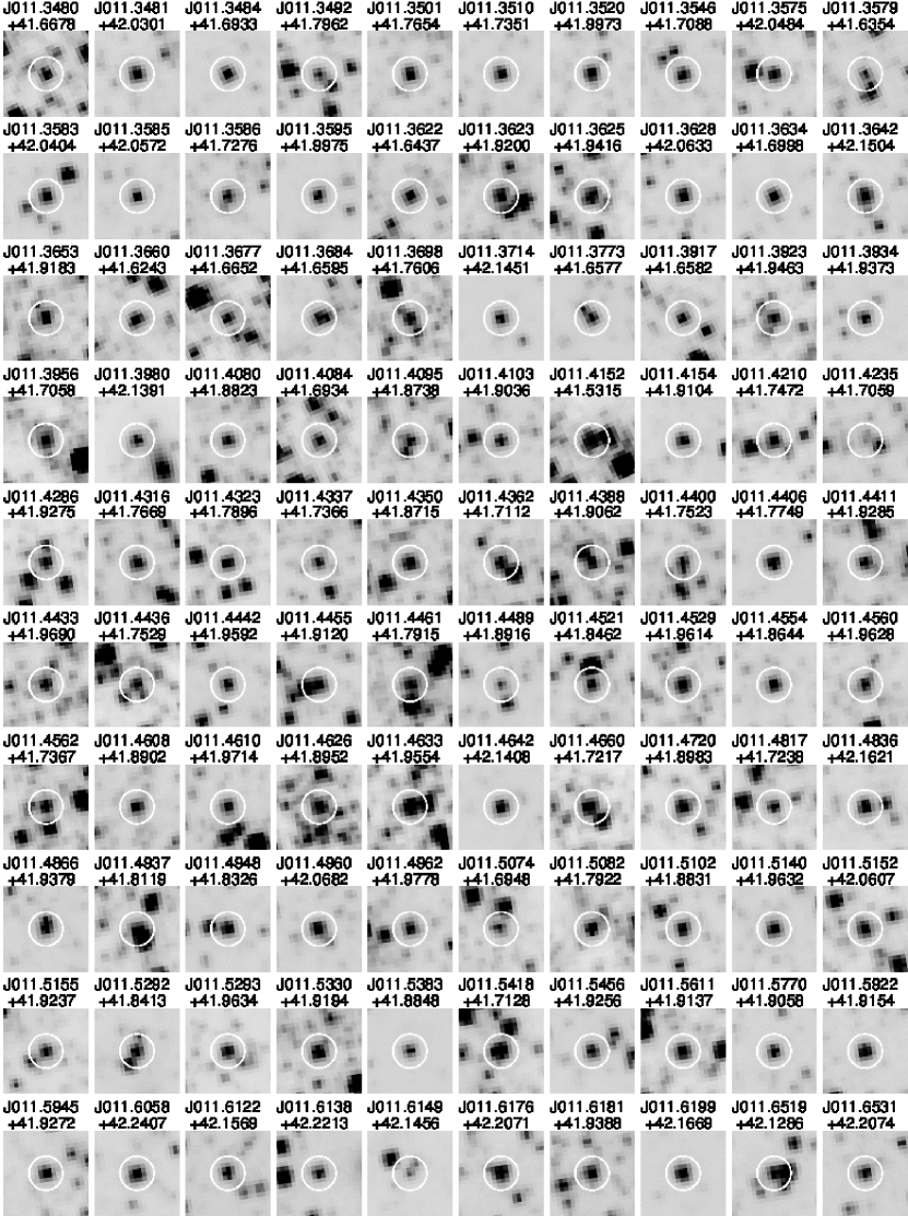
Figure 30: Cepheid stampouts

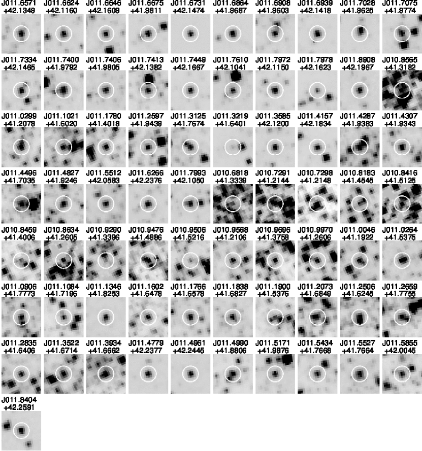
Figure 31: Cepheid stampouts

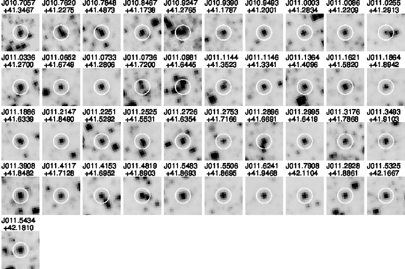
Figure 32: Stampouts of the clipped Cepheids

A.2 Crowding test

This section of the appendix provides Figures (Fig. 33 - Fig. 37) and Tables (Table 4 - Table 6) that include only those Cepheids that have no source closer than 1.5 pixels (c.f. Fig. 2) i.e. are uncrowded. The uncrowded sample consists of 265 Cepheids (217 FM Cepheids, 14 FO Cepheids and 34 type II Cepheids). For this sample 37 Cepheids were clipped (33 FM Cepheids, 3 FO Cepheids and 1 type II Cepheid). The relevant F-test values (c.f. section 4) are $F_{crit}=F(1,268;0.05)=3.88$, $F_{obs,Wesenheit}=8.08$, $F_{obs,F110W}=12.13$ and $F_{obs,F160W}=13.48$. So the broken slopes are still significant at a $2\sigma$ level and the F110W and F160W broken slopes are also still significant at a $3\sigma$ level. Note that the mean F160W offset in Fig. 4 changes to $-0.018~{}\mathrm{mag}$ and the offset in Fig. 5 changes to $-0.257~{}\mathrm{mag}$. Equation 8 changes to

$$\Delta M=<m(\log(P)=1.2)_{\mathrm{R12}}-m(\log(P)=1.2)_{\mathrm{K14}}>=17.689~{}\mathrm{mag}-17.772~{}\mathrm{mag}=-0.083~{}\mathrm{mag}$$ (A1)

which implies for Equation 9:

$$\Delta\mu=(m-M)_{\mathrm{R12}}-(m-M)_{\mathrm{K14}}=\Delta m-\Delta M=-\Delta M=0.083~{}\mathrm{mag}$$ (A2)

and therefore

$$H_{\mathrm{0,K14}}=10^{[\Delta\mu_{0}/5]}\cdot H_{\mathrm{0,R12}}=1.039\cdot H_{\mathrm{0,R12}}$$ (A3)

So the $3.2\%$ increase to $3.9\%$.

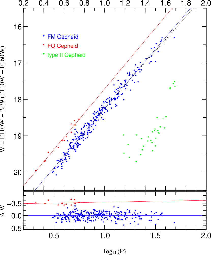
Figure 33: Same as Fig. 7 but only for uncrowded Cepheids (217 FM Cepheids, 14 FO Cepheids and 34 type II Cepheids).

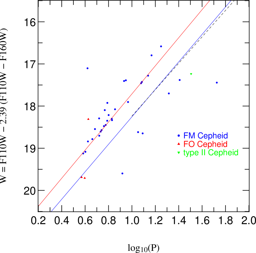
Figure 34: Same as Fig. 8, but only for uncrowded Cepheids. There are 37 clipped Cepheids (33 FM Cepheids, 3 FO Cepheids and 1 type II Cepheid).

Table 4: PLR fit parameters

$\#$	band	type	range	$N_{fit}$	a (log P = 1)	slope b	$\sigma$	$\sigma_{int}$	$\chi_{d.o.f.}^{2}$
1	F110W	FM	all	271	19.515 ( 0.007)	-2.778 ( 0.032)	0.209	-	1.000
2	F110W	FM	log P $>$ 1	93	19.464 ( 0.055)	-2.483 ( 0.155)	0.251	-	1.435
3	F110W	FO	all	14	18.947 ( 0.070)	-2.714 ( 0.152)	0.112	-	1.000
4	F160W	FM	all	271	18.987 ( 0.002)	-2.979 ( 0.023)	0.158	-	1.000
5	F160W	FM	log P $>$ 1	93	18.950 ( 0.023)	-2.755 ( 0.125)	0.184	-	1.348
6	F160W	FO	all	14	18.429 ( 0.072)	-2.973 ( 0.154)	0.087	-	1.000
7	Wesenheit	FM	all	271	18.255 ( 0.005)	-3.259 ( 0.080)	0.137	-	1.000
8	Wesenheit	FM	log P $>$ 1	93	18.236 ( 0.017)	-3.132 ( 0.086)	0.150	-	1.209
9	Wesenheit	FO	all	14	17.712 ( 0.100)	-3.333 ( 0.176)	0.077	-	1.000

Note. — Same as Table 1 but for uncrowded Cepheids.

Table 5: broken slope PLR fit parameters

$\#$	band	$b_{\log(P)\leq 1}$	$b_{\log(P)>1}$	$a_{\log(P)=1}$	$\sigma$	$\chi_{d.o.f.}^{2}$
1	Wesenheit	-3.411 ( 0.058)	-3.077 ( 0.080)	18.219 ( 0.017)	0.135	0.974
2	F110W	-3.071 ( 0.079)	-2.430 ( 0.136)	19.446 ( 0.020)	0.205	0.958
3	F160W	-3.213 ( 0.061)	-2.701 ( 0.103)	18.932 ( 0.015)	0.155	0.952

Note. — Same as Table 2 but for uncrowded Cepheids.

Table 6: parabola PLR fit parameters

$\#$	band	$a_{\log(P)=1}$	$b$	$c$	$\sigma$	$\chi_{d.o.f.}^{2}$
1	Wesenheit	18.233 ( 0.011)	-3.253 ( 0.030)	0.318 ( 0.121)	0.135	0.973
2	F110W	19.475 ( 0.017)	-2.767 ( 0.047)	0.595 ( 0.186)	0.205	0.958
3	F160W	18.955 ( 0.012)	-2.970 ( 0.036)	0.479 ( 0.142)	0.155	0.952

Note. — Same as Table 3 but for uncrowded Cepheids.

Figure 35: Same as Fig. 24 but for 56 uncrowded Cepheids.

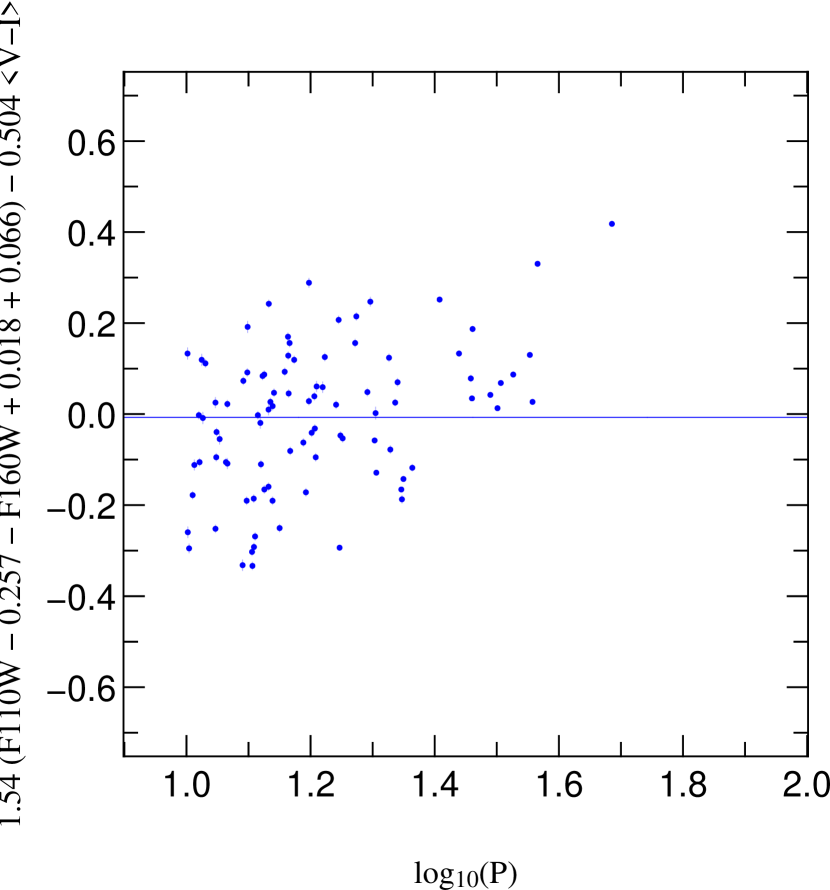
Figure 36: Same as Fig. 25 but for uncrowded Cepheids.

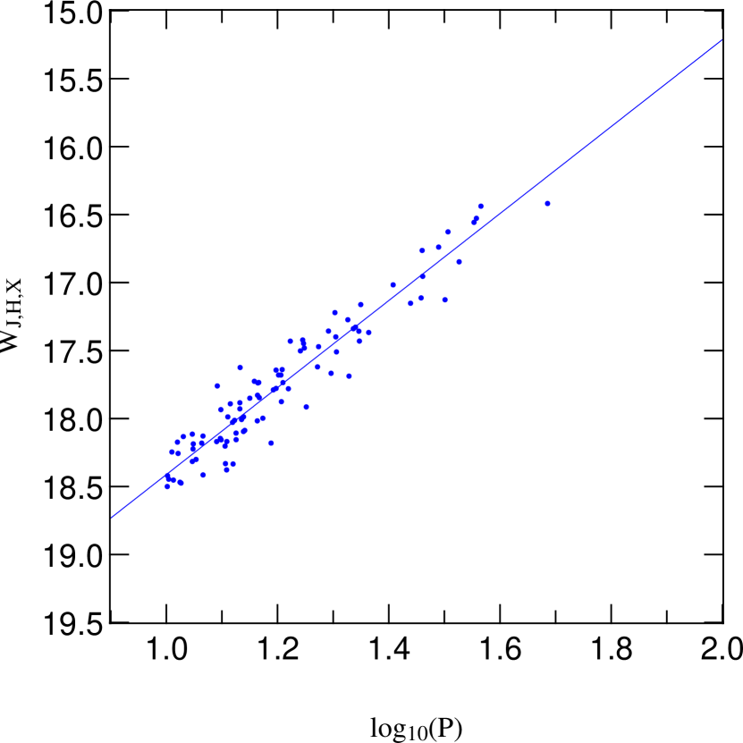
Figure 37: Same as Fig. 26 but for uncrowded Cepheids.

A.3 Suspension point

Due to the fact that our data are random phased we cannot be sure about the correct suspension point. We believe it is better to determine the suspension point with phase corrected data. For the interested reader we provide Table 7 that shows the fit parameters for different suspension points. The best fit for the broken slope is around 8 to 9 days but the observed F-ratio is above the critical F-value for all fits, although also this value favors a suspension point around 8 to 9 days.

Table 7: broken slope PLR fit parameters

$x_{0}$	band	$b_{\log(P)\leq 1}$	$b_{\log(P)>1}$	$a_{\log(P)=1}$	$\sigma$	$\chi_{d.o.f.}^{2}$	$F_{\mathrm{obs}}$
5.000	Wesenheit	-3.813 ( 0.138)	-3.209 ( 0.033)	19.214 ( 0.012)	0.136	0.978	8.195
5.000	F110W	-3.366 ( 0.218)	-2.684 ( 0.056)	20.322 ( 0.020)	0.203	0.988	4.707
5.000	F160W	-3.553 ( 0.166)	-2.904 ( 0.042)	19.858 ( 0.015)	0.154	0.980	7.461
6.000	Wesenheit	-3.598 ( 0.090)	-3.189 ( 0.040)	18.952 ( 0.014)	0.136	0.979	7.845
6.000	F110W	-3.240 ( 0.133)	-2.634 ( 0.064)	20.090 ( 0.020)	0.202	0.979	7.841
6.000	F160W	-3.390 ( 0.087)	-2.866 ( 0.048)	19.613 ( 0.014)	0.153	0.972	10.221
7.000	Wesenheit	-3.508 ( 0.068)	-3.170 ( 0.043)	18.731 ( 0.013)	0.136	0.979	7.710
7.000	F110W	-3.202 ( 0.097)	-2.567 ( 0.072)	19.891 ( 0.020)	0.201	0.965	12.573
7.000	F160W	-3.330 ( 0.068)	-2.819 ( 0.055)	19.405 ( 0.014)	0.152	0.960	14.168
8.000	Wesenheit	-3.474 ( 0.056)	-3.141 ( 0.045)	18.538 ( 0.014)	0.136	0.976	8.923
8.000	F110W	-3.154 ( 0.077)	-2.503 ( 0.079)	19.721 ( 0.020)	0.200	0.955	15.840
8.000	F160W	-3.288 ( 0.057)	-2.770 ( 0.061)	19.225 ( 0.013)	0.151	0.951	17.470
8.500	Wesenheit	-3.455 ( 0.054)	-3.130 ( 0.047)	18.451 ( 0.014)	0.136	0.976	8.959
8.500	F110W	-3.117 ( 0.084)	-2.483 ( 0.085)	19.648 ( 0.020)	0.200	0.955	15.773
8.500	F160W	-3.259 ( 0.050)	-2.754 ( 0.062)	19.147 ( 0.013)	0.151	0.951	17.435
9.000	Wesenheit	-3.440 ( 0.045)	-3.119 ( 0.050)	18.370 ( 0.014)	0.136	0.975	8.969
9.000	F110W	-3.084 ( 0.079)	-2.464 ( 0.090)	19.579 ( 0.020)	0.200	0.956	15.456
9.000	F160W	-3.233 ( 0.051)	-2.739 ( 0.068)	19.073 ( 0.013)	0.151	0.951	17.183
10.000	Wesenheit	-3.411 ( 0.038)	-3.103 ( 0.060)	18.221 ( 0.013)	0.136	0.978	8.237
10.000	F110W	-3.028 ( 0.078)	-2.433 ( 0.105)	19.455 ( 0.021)	0.200	0.960	14.121
10.000	F160W	-3.188 ( 0.050)	-2.714 ( 0.069)	18.938 ( 0.014)	0.152	0.956	15.707
10.470	Wesenheit	-3.399 ( 0.039)	-3.097 ( 0.063)	18.156 ( 0.014)	0.136	0.979	7.723
10.470	F110W	-3.007 ( 0.076)	-2.419 ( 0.112)	19.401 ( 0.022)	0.201	0.962	13.512
10.470	F160W	-3.171 ( 0.048)	-2.703 ( 0.072)	18.880 ( 0.015)	0.152	0.958	14.939
11.000	Wesenheit	-3.386 ( 0.039)	-3.092 ( 0.067)	18.087 ( 0.015)	0.136	0.981	7.140
11.000	F110W	-2.987 ( 0.072)	-2.401 ( 0.116)	19.343 ( 0.022)	0.201	0.963	13.035
11.000	F160W	-3.154 ( 0.047)	-2.691 ( 0.076)	18.817 ( 0.015)	0.152	0.960	14.240
12.000	Wesenheit	-3.365 ( 0.040)	-3.086 ( 0.083)	17.967 ( 0.015)	0.137	0.985	5.971
12.000	F110W	-2.956 ( 0.070)	-2.367 ( 0.119)	19.241 ( 0.022)	0.201	0.965	12.331
12.000	F160W	-3.127 ( 0.040)	-2.668 ( 0.091)	18.707 ( 0.017)	0.152	0.963	13.031
15.000	Wesenheit	-3.325 ( 0.037)	-3.066 ( 0.118)	17.658 ( 0.017)	0.137	0.991	3.977
15.000	F110W	-2.873 ( 0.057)	-2.325 ( 0.190)	18.990 ( 0.026)	0.202	0.978	8.162
15.000	F160W	-3.063 ( 0.044)	-2.636 ( 0.139)	18.432 ( 0.020)	0.153	0.977	8.618

Note. — Same as Fig. 2 but for different suspension points $x_{0}$. Additionally the corresponding $F_{\mathrm{obs}}$ (c.f. section 4) is given.

References

- Anderson King (2006) Anderson, J. King, I. R. 2006, PSFs, Photometry, and Astrometry for the ACS/WFC. (Instrum. Sci. Rep ACS 2006-01; Baltimore: STScI)
- Baranowski et al. (2009) Baranowski, R., Smolec, R., Dimitrov, W., et al. 2009, MNRAS, 396, 2194
- Bono et al. (2010) Bono, G., Caputo, F., Marconi, M., & Musella, I. 2010, ApJ, 715, 277
- Chatterjee & Hadi (2013) Chatterjee, S., & Hadi, A. 2013, Regression Analysis by Example (Wiley)
- Dalcanton et al. (2012) Dalcanton, J. J., Williams, B. F., Lang, D., et al. 2012, ApJS, 200, 18
- Dolphin (2000) Dolphin, A. E. 2000, PASP, 112, 1383
- Efstathiou (2014) Efstathiou, G. 2014, MNRAS, 440, 1138
- Fiorentino et al. (2013) Fiorentino, G., Musella, I., & Marconi, M. 2013, MNRAS, 434, 2866
- Fliri & Valls-Gabaud (2012) Fliri, J., & Valls-Gabaud, D. 2012, Ap&SS, 341, 57
- Freedman & Madore (2010) Freedman, W. L., & Madore, B. F. 2010, ARA&A, 48, 673
- García-Varela et al. (2013) García-Varela, A., Sabogal, B. E., & Ramírez-Tannus, M. C. 2013, MNRAS, 431, 2278
- Inno et al. (2013) Inno, L., Matsunaga, N., Bono, G., et al. 2013, ApJ, 764, 84
- Klagyivik & Szabados (2009) Klagyivik, P., & Szabados, L. 2009, A&A, 504, 959
- Kodric et al. (2013) Kodric, M., Riffeser, A., Hopp, U., et al. 2013, AJ, 145, 106
- Lee et al. (2012) Lee, C.-H., Riffeser, A., Koppenhoefer, J., et al. 2012, AJ, 143, 89
- Madore & Freedman (1991) Madore, B. F., & Freedman, W. L. 1991, PASP, 103, 933
- Madore & Freedman (2012) Madore, B. F., & Freedman, W. L. 2012, ApJ, 744, 132
- Mager et al. (2013) Mager, V. A., Madore, B. F., & Freedman, W. L. 2013, ApJ, 777, 79
- Majaess et al. (2011) Majaess, D., Turner, D., & Gieren, W. 2011, ApJ, 741, L36
- Matsunaga et al. (2009) Matsunaga, N., Feast, M. W., & Menzies, J. W. 2009, MNRAS, 397, 933
- McGonegal et al. (1982) McGonegal, R., McAlary, C. W., Madore, B. F., & McLaren, R. A. 1982, ApJ, 257, L33
- Ngeow et al. (2008) Ngeow, C., Kanbur, S. M., & Nanthakumar, A. 2008, A&A, 477, 621
- Persson et al. (2004) Persson, S. E., Madore, B. F., Krzemiński, W., et al. 2004, AJ, 128, 2239
- Ripepi et al. (2015) Ripepi, V., Moretti, M. I., Marconi, M., et al. 2015, MNRAS, 446, 3034
- Riess et al. (2011) Riess, A. G., Macri, L., Casertano, S., et al. 2011, ApJ, 730, 119
- Riess et al. (2012) Riess, A. G., Fliri, J., & Valls-Gabaud, D. 2012, ApJ, 745, 156
- Sandage (1958) Sandage, A. 1958, ApJ, 127, 513
- Sandage et al. (2006) Sandage, A., Tammann, G. A., Saha, A., et al. 2006, ApJ, 653, 843
- Sandage et al. (2009) Sandage, A., Tammann, G. A., & Reindl, B. 2009, A&A, 493, 471
- Schlafly & Finkbeiner (2011) Schlafly, E. F., & Finkbeiner, D. P. 2011, ApJ, 737, 103
- Udalski et al. (1999) Udalski, A., Soszynski, I., Szymanski, M., et al. 1999, Acta Astron., 49, 223
- Vilardell et al. (2007) Vilardell, F., Jordi, C., & Ribas, I. 2007, A&A, 473, 847