Excitation of Flow Instabilities due to Nonlinear Scale Invariance

Abstract

A novel route to instabilities and turbulence in fluid and plasma flows is presented in kinetic Vlasov-Maxwell model. New kind of flow instabilities is shown to arise due to the availability of new kinetic energy sources which are absent in conventional treatments. The present approach is based on a scale invariant nonlinear analytic formalism developed to address irregular motions on a chaotic attractor or in turbulence in a more coherent manner. We have studied two specific applications of this turbulence generating mechanism. The warm plasma Langmuir wave dispersion relation is shown to become unstable in the presence of these multifractal measures. In the second application, these multifractal measures are shown to induce naturally non-Gaussian i.e. a stretched -Gaussian distribution and anomalous transport for tracer particles from the turbulent advection-diffusion transport equation in a Vlasov plasma flow.

1 Introduction

Relevance of intermittency and multifractal scalings in plasma fluctuations and turbulence have been pointed out in various recent studies. Data analysis based on recent satellite and spaceship measurements reveals that space plasma fluctuations are mostly intermittent in nature with multifractal characteristics [1, 2]. In a fusion plasma edge fluctuations in Stellarators and Tokamaks show that the plasma turbulence is more of an intermittent nature in short time and space scales than in moderate scales when turbulence seems to have a monofractal feature [3]. Intermittency and multifractal fluctuations are also observed in the dynamics of discharge plasma [4]. Significance of multifractal scalings and intermittency were studied in several works in the fluid turbulence [5, 6, 7]. The key feature of the multifractal scaling is the nontrivial dependence of the scaling exponent $\xi(q)$ on a singularity parameter $\epsilon$ that quantifies the strength of singularity in the multifractal measure of the fluctuating dynamical quantity. The symbol $q$, on the other hand, denotes the $q$th moment for the associated probability measure and relates to the singularity parameter $\epsilon$ by a Legendre transform. When the exponent $\xi(q)$ scales linearly with $q$, the fluctuation is purely self-similar, characteristic of a monofractal behaviour. In a more general situation, $\xi(q)$ denotes the generalized dimension spectrum, that is used to classify the observed spatio-temporal fluctuation distributions in various fluid and plasma turbulence and instabilities. Such fluctuation patterns do not conform to self-similarity, but tend, in general, to an intermittent behaviour, i.e. locally analogous to a devil’s staircase function [8]. Understanding the origin and dynamics of such intermittent, multifractal fluctuations in the context of fluid and plasma flows is obviously of considerable interest [5, 6, 7].

In this work we present some new analytic results opening up novel routes to fluid and plasma instabilities [9] which are usually absent in a more conventional analysis of fluid or plasma models. Our study is based on a novel scale invariant nonlinear analysis developed to address in a more coherent manner the production of complex multifractal structures dynamically from a simple initial state. Theory of fractional kinetics [11] using fractional calculus and fractional differential equations are considered by various authors [10, 11, 13, 12] to offer a general theoretical framework to model anomalous scalings and transports. The present approach is not only independent of the fractional kinetics but is a natural extension of the classical analysis to accommodate multifractal scaling behaviours in a smooth (differentiable) manner ([15] -[20]). We show, in particular, how the linear differential measures of the form $dt$ or $dx_{i}$ in a laminar flow can be realized as smooth multifractal measures of the form $dt^{\alpha(\epsilon)}$ and $dx_{i}^{\beta(\epsilon)}$, for a range of multifractal exponents $0<\alpha(\epsilon)\ ,\beta(\epsilon)<1$, in a turbulent flow. The singularity parameter $\epsilon$ corresponds to the scale exposing the level of singularity that is accessed asymptotically and can be related with the Reynolds number in a turbulent flow. The derivation of such anomalous scalings rests on the assumption that increments in a complex flow could be mediated not only by linear shifts but also by small scale discrete, but smooth jumps, giving rise to a duality principle and the associated proliferation of the underlying laminar flow differential equations into self similar replica equations over finer scales . In ordinary setting jump modes are discontinuous, asking for probabilistic arguments to extract macroscopic observables (i.e. the moments) from an irregular Brownian type flow. In the present formalism jump mediated increments are shown to satisfy simple scale invariant linear differential equation in logarithmic variables as opposed to linear shifts of the form $x\mapsto X=x+h$. Although we focus here to applications of this formalism in plasma turbulence, other potential fields of applications are evolution of biological and living systems, stock market variations, dynamics of social systems such as growth and proliferation of human habitats, internet networking, to name a few. We note in particular that the dynamics of a complex organism is known to follow an evolutionary pattern driven mainly by discrete jump mode that is realized, however, in a smooth coherent manner [21] avoiding direct collisions unlike the Brownian motion. The crux of the present approach is to formulate discrete small scale jumps in a smooth manner formally which would allow one to avoid direct collisions with singular points those emerge copiously in the dynamics of a complex system.

It is pertinent to state here the novelty and advantages of the present approach over those available in contemporary literature [10, 11, 12, 13]. As stated already, a major aim is to develop a nonlinear differential analysis to study local behaviour of emergent multifractal measures in turbulent media. The turbulent systems are traditionally studied by stochastic methods [6, 7, 8]. Mathematical models [10, 11, 12, 13] based on fractional calculus, on the other hand, are known to derive anomalous multifractal scaling laws of turbulent flows directly from the underlying fractional differential equations. However, there are various definitions of fractional derivatives such as Riemann-Liouville, Caputo, Weyl, Riezs and others, having relative merits and demerits over each other over their scope and applicability [12]. Moreover, fractional derivatives are basically non-local, thus defeating the very motivation of using a differential equation to discuss local structures. The present approach, however, formulates a rigorous framework of using integer-order differential equations based instead on multifractal measures for local descriptions of evolutionary patterns of emergent complex systems. The differential equations valid for simple systems or in a laminar flow condition are shown to replicate self similarly on the emergent multifractal structures signaling onset of turbulence.

To explain emergence of anomalous multifractal scalings specifically in a turbulent plasma, we first discuss how the scaling of a dynamical variable may become anomalous due to novel multifractal contributions from the asymptotic boundary layer regions realized in a self consistent manner in a given fluid model. Such anomalous scalings can be interpreted as the production in abundance of spatio-temporal multifractal measures [5] triggering turbulence generating instabilities even in a simple electrostatic plane wave solution of the kinetic Vlasov-Maxwell system [9]. As an another application of this novel nonclassical measure, we next derive anomalous stretched Gaussian scalings [11, 13, 10] for the transport of charged tracer particle distribution in a turbulent Vlasov plasma.

2 Nonclassical Measures in Fluid

Here, we present in brief the mathematical arguments [17, 19, 20] leading to the emergence of multifractal scalings from standard differential measures in a laminar flow as the original laminar flow tends to become turbulent. Recall that the traditional (differential) Lebesgue measure is well suited for simple systems, for instance, the uniform rolling of a billiard ball along a straight line, say, or in a laminar flow. In such a context if one envisages a limiting statement involving $x\rightarrow x_{0}$ ($x$ may denote the position of the ball), then it is reasonably correct to treat this motion using the ordinary measure $\Delta x=x-x_{0}$ which goes to zero linearly with uniform rate 1. Motion of a single fluid particle in a moving or static body of fluid medium (Lagrangian view), however, is likely to present a new caveat. As the fluid particle moves uniformly along a streamline (actually a path line) of a laminar flow of the fluid medium, the standard Lebesgue measure apparently has to be modified because of a possible back reaction generated by the intervening fluid particles in the medium. In a laminar flow such back reactions would of course be negligible and can safely be ignored. However, in a turbulent flow the said back reactions from intervening fluid particles (molecules) need not be negligible. The line segment joining any two points along a turbulent path line, $x$ and $x_{0}$ say, would develop more and more into an irregular curve as the particle at position $x$ is transported non-uniformly not only linearly but also through infinitesimal smooth jumps avoiding singularities those are created dynamically by the enhanced pressure generated within the flow. The length of the dynamically generated irregular curve in the intervening medium, which would grow indefinitely, would, however, contribute a finite (renormalized) correction term to the ordinary Lebesgue measure akin to the renormalization group [22] actions delivering a finite observable effect from an apparent divergence (Fig.1). More importantly, this accumulation of an extra measure is realized in a manner consistent with the original dynamical constraints of the motion.

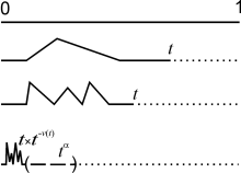
Figure 1: Nonlinear Limit: As a variable $t$ in fluid model approaches 0, the length of invisible (inaccessible)) sector $(0,t)$ diverges intermittently as $t\times t^{-\nu(t)}$. In the limit $t\rightarrow 0$, the neighbourhood of 0 in the visible (accessible) sector $t>0$ is extended by a duality principle to a totally disconnected multifractal set and the original variable $t$ is replaced by the effective renormalized variable $t^{\alpha}$, where the multifractal scaling exponent $\alpha=\alpha(\eta)$ corresponds to the singularity spectrum of the associated multifractal measure. The effective variable $t^{\alpha}$ does not vanish even when $t$ goes to zero (see text for details).

2.1 First Derivation

To explain the above mentioned emergence of the nonclassical measure, let us suppose that the dynamic variable $t$, greater than 1 initially, approaches 0 from the right. For definiteness we assume that the variable $t$ is dimensionless in the sense that $t$ satisfies the scale invariant equation

$$t\frac{dx}{dt}=x,\ x(1)=1$$ (1)

The variable $x$ here may denote the position of a test particle in a uniformly flowing fluid. Assume also that the real number line has a soft, fluid like structure (one dimensional and may be static) so that as $t>0$ approaches 0 the segment between 0 and $t$ gets squeezed in the form of an irregular curve. The length of this segment would grow indefinitely, supposedly in the form $t\times t^{-\nu(t)}$, as $t$ closes gradually toward 0 and continues to become vanishingly small, but does not vanish exactly (0 being a singular point, that may be present in a specific physical problem or fabricated dynamically, see below). As long as $t$ approaches 0 linearly as in an uniform laminar flow the factor $t^{-\nu(t)}$ would remain constant ($\approx 1$) so that $\nu(t)$ satisfies the scale invariant equation

$$\log t\frac{d\nu}{d\log t}=-\nu$$ (2)

and $\nu(t)=\frac{k_{0}}{\log t}$, $k_{0}>\approx 0$ being a constant. However, as the line segment $(0,t)$ gets gradually squeezed due to effective compressive force generated by the nonlinear flow, we expect formation of a countable set of singular points where $\nu(t)$ is nondifferentiable in the usual sense. The length (measure) of the dynamically generated irregular curve inside the interval $(0,t)$ would, however, grow gradually with the production of more and more singularities in the interior. In the present approach such a possibility of dynamic production of a singularity set is avoided, so to speak, by allowing the flow variable $t$ to execute smooth smaller scale jumps respecting eq(2) and its dual eq(3).

First, let us establish the successive growth of length of the interval $(0,t)$ with the generation of $n$ number of singular points $t_{i}:\ i=1,2,\ldots$ such that $0<t_{i+1}<t_{i}<t$. To begin with, suppose $t_{1}$ be the first singularity produced as the line segment $(0,t)$ is squeezed slightly. Exploiting the scale invariance, the exponent $\nu(t)$ would now satisfy eq(2) with $t$ replaced by the rescaled variable $\tilde{t}=t/t_{1}>1$ so that we have $\nu(t)=\frac{k_{1}}{\log\tilde{t}}$, $k_{1}>k_{0}$, and the length of the intervening fluid line would grow as $te^{k_{1}}>t$. At the next level of squeezing, one considers generation of two singular points $0<t_{2}<t_{1}<t$. Proceeding exactly as above with the rescaled variable $t\mapsto\tilde{\tilde{t}}=t/t_{2}$ instead, one now arrives at an enhanced length of the form $t\times t^{-\nu}=te^{k_{2}},\ k_{2}>k_{1}$. Notice that $k_{2}<k_{1}$ is inconsistent with the proposed scenario. Thus with the production of more and more number of singular points the linear measure $t$ of the original segment $(0,t)$ would continue to grow multiplicatively as $te^{k_{n}}$, $k_{n}\rightarrow\infty$ as $n\rightarrow\infty$, when the $n$th level singularity $t_{n}$ is mapped to $t=1$ by rescaling $t/t_{n}$. It follows, consequently, that the nature of the generic singularity at $t=1$ should alter successively as singularities from far deeper regions of $(0,t)$ are mapped to $t=1$ by rescalings. To conclude, the diverging growth in measure in the interior of the fluid segment $(-t,t)$ could be modeled by the simple, logarithmically scale invariant eq(2). The scaling exponent $\nu(t)=\frac{k_{n}}{\log{t^{\prime}}}>1,\ t^{\prime}=t/t_{n}>1$ would diverge in an intermittent manner as new singularity at $t_{n+1}$ is met as $t\rightarrow 0$ by squeezing. This dynamical emergence of singularity set and the associated diverging growth in measure is, however, eliminated (or avoided) by invoking the principle of duality and inversion mediated jump modes as outlined below.

To see explicitly this avoidance of singularity, suppose $t=1$ is the dynamically generated singularity as $t\rightarrow 0$ nonuniformly as described above. As noted already, singularity at any arbitrary point $0<t_{0}<t$ can be mapped to $t=1$ by scale invariance, so that the description of jump mode in the neighbourhood of $t=1$ can be taken as generic. In the said neighbourhood of the singular point 1, let us consider two unevenly distributed points $t_{-}<1<t_{+}$, $t_{+}=1+\eta$ and $t_{-}=1-g(\eta),\ g(\eta)\gtrapprox 0$ for $\eta\gtrapprox 0$ with the property that $0<g(\eta)<\eta$. By transition via inversion induced small scale jump we mean $t_{+}\mapsto t_{+}^{-1}=t_{-}$, so that the exponent $\nu(t_{+})\mapsto\nu(t_{-})=\nu(t_{+}^{-1})\propto 1/\nu(t_{+})$. As a consequence eq(2) valid in the right neighbourhood of 1 gets transformed into a dually (inversely) related self similar replica

$$\log t\frac{d\nu}{d\log t}=-\nu\ \longmapsto\ \log t\frac{d\nu}{d\log t}=\nu$$ (3)

leading to $\nu(t_{-})=k\log t_{-}^{-1},\ k>0$. Notice that had the point $t=1$ been regular, eq(2) would have been extended over the left neighbourhood as well. To emphasize, we see that the dual eq(3) is essentially the self similar replication of the original eq(2) by inversion in classically forbidden (that is to say, inaccessible) region of the turbulent flow.

In presence of this nontrivial jump mode, we now see that the effective scaling factor $t_{+}^{-\nu(t_{+})}$ that remains locally constant in the right hand side of the singular point $t=1$ would make a smooth transition to a fluctuating variable $\tau=t_{-}^{-\nu(t_{-})}$ by inversion induced jump. As $t_{+}\rightarrow 1$, the locally constant scale factor becomes a fluctuating variable $\tau\approx t_{-}^{-kg(\eta)}=t^{-\frac{k(g(\eta))^{2}}{\log t^{-1}}},\ t\approx 0$ for a class of scaling functions $g(\eta)=\eta^{s},\ \eta>0$. The exponent $0<s<1$ depends on the nature of the singularity point. Since there could at least be a countable set of singularities in the interval $(0,t)$ for any small but finite value of $t$, $g(\eta)$ actually denotes a multifractal scaling function. As a consequence, in the limit $t\rightarrow 0$, the ordinary laminar flow measure $dt$ is transformed into the smooth multifractal measure $dt^{\alpha(\eta)}$ where $0<\alpha(\eta)=1-\frac{k(g(\eta))^{2}}{\log t^{-1}}<1$ varies over the singularity set of $(0,t)$. As, in the limit $t\rightarrow 0$, there are an uncountable number of possible singularity set (essentially, a family of Cantor sets), exponent $\alpha$ represents a huge spectrum of turbulent fluctuations. It should be clear that the exponent $\alpha(\eta)$ has intermittent behaviour being almost constant slightly away i.e. as $g(\eta)\rightarrow\eta$ (so that $s\rightarrow 1$ and $\alpha(\eta)\approx 1$ as $\frac{k\eta^{2}}{\log t^{-1}}\approx 0$ relative to the first order infinitesimal $\eta$), from the singular point.

We remark that the dimensionless variable $t$ may either be the time variable or a space variable. The turbulent differential measure for a space variable would scale as $dx^{\beta(\eta)}$ for a multifractal exponent $0<\beta<1$.

Relationship with classical multifractal measure: A multifractal set is a set that is composed with a multitude of interwoven fractal subsets, each with differing fractal dimension [8]. The fractal dimension $D$ gives the idea of scaling of a measure $\mu$ with support on the fractal set $F$ with the size $\delta$ of a ball $B_{x}(\delta)$ centered at $x\in F\cap B_{x}(\delta)$: $\mu(B_{x}(\delta))\sim\delta^{-D}$. The fractal dimension $D$ is defined globally as a constant for a fractal set. For a multifractal the above scaling can be valid only locally: $\mu(B_{x}(\delta))\sim\delta^{\epsilon(x)}$. Here, the exponent $\epsilon(x)$ denotes the singularity strength at the point $x$ and does not, in general, define the fractal dimension of any set. To generalize the concept of dimension for a multifractal set, there exist two approaches, related, in a sense, by a Legendre transform. The first approach starts by covering the support of multifractal measure by boxes of size $\delta$. Let $N_{\epsilon}(\delta)$ be the number of boxes that scales like $\delta^{\epsilon}$. Then, under mild restrictions [14], it can be shown that there exists a convex function $\alpha(\epsilon)$ such that $N_{\epsilon}(\delta)\sim\delta^{-\alpha(\epsilon)}$ and the exponent $\alpha(\epsilon)$, called the singularity spectrum of the multifractal measure, has the interpretation of the fractal (box or Hausdorff) dimension of an interwoven set of points $x$ having the singularity strength $\epsilon(x)=\epsilon$.

In an alternative approach, one considers the partition function $S_{\delta}(q)=\sum_{i}\mu(B_{i}(\delta))^{q}$ for the support of the probability measure $\mu$ that is covered by the balls $B_{i}$. Again, under the stated mild conditions, the partition function has a power law scaling $S_{\delta}(q)\sim\delta^{\tau(q)}$ for $\delta\rightarrow 0$ and one arrives at the generalized Renyi dimensions $D_{q}=\tau(q)/(q-1)$. Further, the generalized dimension spectrum $\tau(q)$ relates to the singularity spectrum $\alpha(\epsilon)$ by the Legendre transform $\tau(q)=\underset{\epsilon}{\inf}{(q\epsilon-\alpha(\epsilon))}$.

To interpret the smooth multifractal scaling exponent $\alpha(\eta)$, derived above from the inversion mediated jump modes, as the singularity spectrum of the dynamically generated multifractal measure in the soft model we proceed as follows. The neighbourhood of the generic singularity at $t=1$ is extended, by rescalings, into non-classical multifractal set that is covered by open intervals (balls) of size $\delta$. The measure concentrated on such a ball scales locally as $\delta^{\eta(\tau)}$. Here, the rescaled variable $\tau$ belongs to the multifractal set and relates logarithmically to the original variable $t$ in the vicinity of the generic singularity. The singularity parameter $\eta(\tau)$ gives an estimate of the relative size of miniscule connected segments over a distribution of miniscule open gaps in the neighbourhood of the point $\tau$ (c.f. Sec.2.3). The exponent $\alpha(\eta)$ now have the meaning of the singularity spectrum of the underlying multifractal measure that is generated dynamically from the diverging linear measure in the invisible (inaccessible) sector in the neighbourhood of the singularity at $t=1$ by the duality principle enunciated above. We shall, however, continue to call the exponents $\alpha(\eta)$ and $\beta(\eta)$ loosely as multifractal scaling exponents in what follows.

2.2 Alternative derivation

We give here another derivation of the jump mediated multifractal increments to explain the origin of turbulent like behaviour in an asymptotic time as $t\rightarrow\infty$. This also points out the appearance of smaller and larger scales dynamically thus making room for activation of jump modes in an otherwise featureless flow. Since we are concerned with realizing a (scale invariant) nonlinear increment in a fluid medium from a linear laminar flow, let us consider the simplest scale invariant uniformly accelerated flow equation

$$t\frac{dv}{dt}=v,\ v(1)=1$$ (4)

in a bounded region of the form $\epsilon<t<\epsilon^{-1}$ where $\epsilon$ may relate to a sufficiently distant time scale $T=\epsilon^{-1/a},\ 0<a=a(\epsilon)<1$. The exponent $a$ is reminiscent of an anomalous scaling that will be justified below. In a simple, laminar like flow condition, the conventional linear velocity increment of the form $\Delta v=v(t+h)-v(t)$ works perfectly well in a fluid model and we also have $a=1$. However, a turbulent like condition may be mimicked here even by eq(4) when one considers a singular limiting problem defined by the concomitant limit $t\rightarrow\epsilon^{-1}$, but $\epsilon\rightarrow 0$ satisfying the condition $0<\epsilon<t^{-1}$. This singular problem is indeed nonclassical because of availability of infinitely large scales of the form $\tau>1$, when the classical analysis can have only to ordinary scales $1\leq t<1/\epsilon$. In the present nonclassical approach, the point $\tau=\epsilon t=1$ is a singularity that is unattainable classically as $t\rightarrow\infty$. However, in the extended scenario, increments in a deleted neighbourhood of $\tau=1$ can be realized by an inversion of the form

$$\tau_{-}=\epsilon t\ (<1)\mapsto\tau_{-}^{-1}=\tau_{+}=t^{-\alpha(\epsilon)}$$ (5)

where we set $\epsilon t^{a}=1$, in the limit $t\rightarrow\infty$ and $0<\alpha(\epsilon)=1-a(\epsilon)<1$, thus transferring an element at $\tau_{-}<1$ to $\tau_{+}>1$, on the extended rescaled real line, instantaneously by the nonlinear but smooth jump mode. More importantly, above inversion induced scaling scenario provides an automatic scheme for identifying the disconnected right neighbourhood of $\tau=1$ with the right neighbourhood of $\tau=0$ of the real line $0<t<\epsilon^{-1}$. We rewrite this new rescaled inverted variable in the right neighbourhood of 0 by $t_{1}=t^{-\alpha(\epsilon)}$. Next, we notice that inversion induced increments as above satisfies eq(4), viz., $t\frac{dv}{dt}=v$, in the transformed small scale monotonic variable $t_{1}=t^{-\alpha(\epsilon)}\gtrapprox 0$ when the ordinary differential increments are translation invariant. As a consequence the inversion induced increments may be said to be translation invariant in double logarithmic variable $\eta=\log\log t_{1}$ when increments are taken as $\log h,\ 0<h<1$.

In a turbulent flow small/large scale nonlinear jump increments given by eq(5) are likely to play vital, predominant role over the ordinary linear increments. Multiscale coherent structures such as eddies and vortices generally endow a turbulent medium a multifractal structure leading to nonuniform scaling exponents and intermittency. In the present approach the jump mode scaling exponent $\alpha=\alpha(\epsilon)$ is not necessarily a fixed constant but a variable depending on the level of singularity, that is to say, the regions or levels of scale changes as encoded explicitly by $\epsilon$ and hence corresponds actually to a multifractal scaling in the turbulent flow (c.f. Sec.2.1). More importantly, a fixed exponent $\alpha$ can only be locally constant in the sense that $\alpha$ is constant for the time scale $t_{1}<<\epsilon^{-1}$ only, but may vary in the next generation large scale $t_{1}\sim\epsilon^{-1}$, and so on. To see this explicitly, suppose $K$ is a constant i.e. $\frac{dK}{dt}=0$ for $\epsilon<t<<\epsilon^{-1}$. However, as $t\rightarrow T^{a}=\epsilon^{-1}$ one gets $\epsilon\frac{dK}{d\epsilon t}=0$ and so by letting $\epsilon\rightarrow 0$ one may deduce that $\frac{dK}{dt_{1}}\neq 0$, when we make use of the jump mode transformations eq(5). So we conclude that

$$K=\mathrm{const.,\ for}\ \epsilon<t<\epsilon^{-1};\\ \mathrm{but}\ \frac{dK}{dt}\neq 0,\ \mathrm{when}\ t\gtrapprox 1/\epsilon$$ (6)

because of the dynamical production of multifractal measures abundantly in the asymptotic boundary layer regions.

Let us recall that in the literature of singular perturbation methods [22], one considers a limiting ansatz of the form $(\tau_{-}=)\ \epsilon t=\epsilon^{-b},\ b=b(\epsilon,t)$ which can be rewritten as $\tau_{-}=t^{\frac{b\log\epsilon^{-1}}{\log t}}$ so that under the proposed inversion mediated jump, one obtains $\tau_{+}=\tau_{-}^{-1}=t^{-\frac{\log t}{b\log\epsilon^{-1}}}$, which exactly matches the derivations of Sec.2.1 following the duality principle viz, eq(3), and also with eq(5) for $\alpha(\epsilon)=\frac{\log t}{b\log\epsilon^{-1}}$. This also tells that the duality is already incorporated into the definition of $\alpha(\epsilon)$ (see below), so that explicit realization of the duality via eq(3) is not necessary in writing eq(5). In other words, the exponent $\alpha(\epsilon)$ is an effective renormalized quantity, invariant under the duality transformation.

Finally, to justify the anomalous scaling for $t$ as $t\rightarrow\infty$ in the present formalism let us remark that as $\eta=t^{-1}\rightarrow 0$ respecting $0<\tilde{\eta}_{n}<\epsilon^{n}<t^{-1}$, relatively invisible smaller scales $\tilde{\eta}_{n}$ residing in $(0,\epsilon^{n})$ might have a coherent, cooperative effect on the visible variable $\eta$ in the form $\eta^{-\alpha(\epsilon)}$ where the slowly varying, locally constant effective exponent $\alpha(\epsilon)=\underset{n\rightarrow\infty}{\lim}\log_{\epsilon^{-n}}(\epsilon^{n}/\tilde{\eta}_{n})>0$ is interpreted as an ultrametric valuation living in a multifractal set of microscopically small and macroscopically large scales [18, 19, 20]. Clearly, cascades of infinitesimally small scale invisible elements $\tilde{\eta}_{n}$ are related dually (i.e. inversely) to a visible, limiting element $\eta$, and hence this definition of the scaling exponent $\alpha(\epsilon)$ naturally incorporates the duality transformation eq(3). A complex turbulent flow is likely to generate such a multifractal set abundantly. Notice that the valuation $\alpha(\epsilon)$ is nontrivial, even when the ordinary variable $\eta$ vanishes asymptotically and signifies cooperative effects of smaller (invisible) scales in formation of complex structures by the inversion induced duality principle. In Sec.2.1, dynamically generated scaling exponent $\alpha(\epsilon)$ is interpreted as the singularity spectrum of the associated multifractal set.

To give an explicit example of the above remarks, let us suppose that the ordinary linear limiting variable $\eta\rightarrow 0$ acquires a nonlinear structure, of the form $\eta\mapsto\eta^{\prime}=\eta^{1-\alpha}$, by the limiting duality $\tilde{\eta}_{n}/\eta^{n}\propto(\eta/\eta^{\prime})^{n},\ n\rightarrow\infty$, so that $0<\alpha(\eta)=\frac{\log\eta/\tilde{\eta}}{\log\eta^{-1}}=\underset{n\rightarrow\infty}{\lim}\frac{\log\eta^{n}/\tilde{\eta}_{n}}{\log\eta^{-n}}<1$ where $\tilde{\eta}=\underset{n\rightarrow\infty}{\lim}\tilde{\eta}_{n}^{1/n}$, for the smaller scale cascade $0<\tilde{\eta}_{n}<\eta^{n}$. Nontriviality of the valuation $\alpha(\eta)$ is verified by setting $\alpha(\eta)=\alpha_{0}$, a constant for all $\eta\in(0,1)$, so that $\alpha(\eta)$ trivially is an ultrametric. More generally, $\alpha(\eta)=\alpha_{0}\eta^{s(\eta)}$ is locally constant over countable open subintervals of (0,1) (i.e. $\eta^{s(\eta)}={\rm constant}$), with nontrivial variability at the points of (classical) discontinuity, as represented by the variable factor $\eta^{s(\eta)}$ with $s(\eta)=s$ remaining constant on an infinitesimally small subinterval of the set of variability of $\alpha(\eta)$ [19, 20], reflecting the cooperative effects of smaller scale cascades. The effective renormalized exponent $\alpha(\eta)$ thus has an intermittent behaviour as claimed. For a special set of values of the form $\eta=1/3^{m\log 3},\ \tilde{\eta}=\eta\times 1/3^{m\log 2},\ m>0$ , the scaling exponent $\alpha(\eta)=\frac{\log 2}{\log 3}$ represents dynamical formation of a monofractal, i.e. the classical triadic Cantor set of dimension $\alpha_{0}=\frac{\log 2}{\log 3}$ in the neighbourhood of the singular point 0. For a realistic nonlinear flow such a well patterned set of values are exceptional, leading instead to an intermittent multifractal exponent $\alpha$ depending on $\eta$.

An important feature to the above derivations, as remarked already in Sec.2.1 is that the above multifractal measure is valid both in the time and space domains. Ordinary Lebesgue measure $dx$ (say) is now extended to the nonlinear multifractal measure of the form $d_{m}x:=dX^{-1}=dx^{\beta(\epsilon)},\ 0<\beta<1$, since in the far asymptotic limit considered here linear increment $x\mapsto x+h$ gets extended to the nonlinear increment $x\mapsto x+h^{\beta}$. Here, $X^{-1}=x^{\beta(\epsilon)}$ denotes the nonclassical space variable extension (by inversion induced duality principle) in an arbitrarily small neighbourhood of $x=0$, analogous to the time variable $T^{-1}$ near $t=0$. The neighbourhood of $x=0$ is said to have extended into a totally disconnected multifractal set since the exponent $\beta(\epsilon)$ is defined only locally and satisfies the inequality $0<\beta(\epsilon)<1$. An equation of the form eq(1) on a connected line segment close to 0 would then be replicated self similarly, by the said duality, on infinitesimally small disconnected line segments in an appropriate nonclassical variable of the form $T^{-1}$ or in $X^{-1}$. The novel possibility of such nonlinear transitions would have significance in offering new inputs in the study of instabilities and turbulence.

Before closing this Section, let us point out that the production of multifractal measures in abundance in both space and time coordinate spaces in a fluid medium has an interesting physical (dynamical) interpretation. In a high Reynolds number flow, the relative velocity between two contiguous fluid elements is expected to be very high. As the separation (usual Lebesgue sense) of the fluid elements is reduced to an infinitesimal level denoted by the fiducial scale $\epsilon$, the diverging nonlinear measure, activated in the intermediate fluid medium because of generation of very high contractive forces by dragging effects in the high velocity flow, leave an influence in the form of a finite effective multifractal measure in the observable sector by inversion. The continuum fluid medium at the invisible infinitesimal scales $<\ \epsilon$ appears to have assumed asymptotically the granular structure with a diverging measure. The freedom of inversion mediated transfer of enhanced measure, that is to say, kinetic energy from the invisible sector to the observable dynamical sector $>\ \epsilon$ in the present scenario creates the room for realizing new levels of instabilities and complex flow patterns in the fluid. The present inversion mediated energy enhancement is analogous in spirit of the renormalization group techniques in critical phenomena and nonlinear systems [22]. The detailed comparison of the two approaches in the fluid flow would be considered separately.

2.3 Activation of Jump Mode: Definitions

Here we introduce the formal definition of the inversion induced jump modes. As before we consider two points $t_{\pm}=1\pm\eta,\ {\rm and}\ t_{+\mu}=1+\eta\mu(\eta),\ \eta<<1$ in the vicinity of $t=1$ which may or may not be a singularity for a flow. Further, let us we assume here that $t_{-}\mapsto t_{-}^{-1}=\lambda t_{+\mu}$, which is the definition of an inversion induced jump transferring the point at $t_{-}$ to a spectrum of possible points denoted by $t_{+\mu}$ and $\lambda$. Our aim is to spell out the role of each of the parameters involved in the definition. We first note that $t_{-}^{-1}=1+\frac{\eta}{1-\eta}:=\tilde{t}_{+}>t_{+}$, a unique point in the right hand side of $t=1$. In case $t=1$ is regular, all the above points attain the point $t=1$ as $O(\eta)$ when $\eta\rightarrow 0$. The linear increment corresponding to inversion induced transition is $\Delta_{i}t_{-}=t_{-}^{-1}-t_{-}=\frac{\eta(2-\eta)}{1-\eta}\sim O(\eta)$. Noting that linear increment for shift mediated flow from $t_{-}$ to $t_{+}$ is $\Delta t_{-}=t_{+}-t_{-}=2\eta$, the relative gain in the jump mediated increment over the ordinary shift defined by $\Delta_{j}t_{-}=(\Delta_{i}t_{-}-\Delta t_{-})/\Delta t_{-}=O(\eta)$ vanishes as $\eta\rightarrow 0$. As a consequence, in a regular flow the measure of the activation of jump modes over the linear mode, defined as the logarithm of the rate of variation of the relative gain of jump mediated increment over the usual linear increment, viz. $J=\log_{\Delta t_{-}}(\Delta_{j}t_{-}/\Delta t_{-})$, vanishes in the limit $\eta\rightarrow 0$. Hence forth, we call $\Delta_{j}t$ the pure jump increment at the point $t$ and evaluated asymptotically in an open neighbourhood of the form $(t-t\eta,t+t\eta)$ when $\eta\rightarrow 0\ (\neq 0)$.

In the nontrivial case, when $t=1$ is a singularity, developed dynamically in a flow, the first order infinitesimal $\eta$ can approach 0 arbitrarily close but, nevertheless, fails to reach 0 exactly. In this case we demonstrate a nontrivial activation of a jump mode asymptotically as $\eta\rightarrow 0$.

As $t_{-}\rightarrow 1$, nonlinear back reaction from the singularity creates a room to invoke jump mode so that the dynamical variable $t$ at $\tilde{t}_{-}=1-\eta\mu(\eta)=t_{-}^{\mu(\eta)}+O(\eta^{2}),\ \mu(\eta)<1,\eta<<1$ takes a jump $\tilde{t}_{-}\mapsto\tilde{t}_{-}^{-1}\propto t_{+}$ to bypass the singularity and thus to allow the flow to continue smoothly but with added structures for $t>1$. As a consequence, the small scale variable $\eta$ in the right hand side of the singularity denotes a growing variable in the interval (0,1). The above relation can be rewritten in the equivalent form of a jump mode introduced previously (c.f. Sec.2.1): $t_{-}\mapsto t_{-}^{-1}=\lambda t_{+\mu^{-1}}+O(\eta^{2})=\lambda(1+\eta\mu^{-1}(\eta))+O(\eta^{2}),\ \lambda<1$. The function $\mu$ is assumed to belong to the class of sufficiently differentiable functions for $\eta>0$ that represents non-specificity or uncertainty in the exact moment in realizing a jump before an emerging singularity. The proportionality parameter $\lambda$ denotes possible uncertainty in the final moment. The combined effect of uncertainty now is rewritten as $t_{-}^{-1}=t_{+}^{\nu}+O(\eta^{2})$ where $\nu=\mu^{-1}+\frac{\log\lambda}{\log t_{+}}$. For definiteness we assume $\nu>1$. This corresponds to continuity of flow and associated structure formation induced by the singularity as referred to above.

It now follows that the jump increment $\Delta_{j}t_{-}$, in the nontrivial case, has the form $\Delta_{j}t_{-}=\frac{1}{2}(\nu-1)+O(\eta)$. In the presence of a singularity at $t=1$, one may imagine an open gap of the form $(1-\eta,1+\eta)$ that is crossed by a jump. The above jump increment then gives a measure of the size of a compact connected segment determined by $\nu$ relative to the open gap of size $2\eta$. Because of intrinsic scale invariance of the jump mode (c.f. Sec. 2.1), a class of nontrivial jump modes is determined uniquely by $\nu=1+2\eta^{\alpha},\ \eta>0$ where $0<\alpha(\eta)<1$. The associated nonlinear differential measure for jump mediated flow is defined by $d_{j}t=d{\tilde{t}}^{\alpha(t)}$ where $\tilde{t}\approx 0$ is a scale invariant small scale growing variable in the neighbourhood of a singularity. As a consequence, the ordinary measure $dt$ gets extended to the nonclassical measure $dT$ for $T=t(1+{\tilde{t}}^{\alpha}/t)$ where the nontrivial part, representing smooth intermittent fluctuations, is activated only in a small neighbourhood of a singularity when $\tilde{t}\approx 0$ but never vanishes exactly. It also follows that the corresponding activation parameter $J=\log_{\Delta t_{-}}\frac{1}{\Delta t_{-}}\Delta_{j}t_{-}=(1-\alpha),\ \alpha\neq 1$ relates to the dimension of the multifractal set on which jump modes live. This activation parameter has an equivalent ultrametric interpretation [18, 19, 20] and was referred to in Sec.2.2.

To summarize, we have presented two different routes for derivation of multifractal differential measures from a soft (fluid) model of real line. It is argued that the linear Lebesgue measure follows from the ordinary stiff model of real line and should apply or be relevant for laminar type flow only. In a complex turbulent flow Lebesgue measures of the form $dt$ and $dx$ must be extended to multifractal measures of the form $dt^{\alpha(\epsilon)}$ and $dx^{\beta(\epsilon)}$ signifying dynamical onset of multifractal sets in the turbulent flow. The exponents $\alpha(\epsilon)$ and $\beta(\epsilon)$ correspond to the singularity spectra of the multifractal measures in the time and space domains respectively of the nonlinear flow. The first derivation of the multifractal measures makes use of a duality principle in the context of the scale invariant equations eq(2) and eq(3). The alternative approach is based on an effective valuation that is invariant under the jump mediated duality transformation. The formal definitions of jump increment and the associated jump differentials are presented in Sec.2.3. A measure called the activation parameter $J$ is also introduced, non-triviality of which demonstrates the onset of nonlinear incremental modes in the flow. It also follows that the jump increment for $t$ ( or $x$) in the neighbourhood of $t=1$ ( or $x=1$) corresponds to the ordinary increment for the scaling function $(\log t)^{\alpha(\epsilon)}$ ( or $(\log x)^{\beta(\epsilon)}$), $0<\alpha(\epsilon)<1\ (0<\beta(\epsilon)<1))$.

3 Applications to Plasma

Here we present two applications of the above formalism in plasma instabilities and plasma turbulence. These examples are expected to confirm that the instabilities considered here actually belong to altogether a new class of instabilities that plague any linear and nonlinear system. We consider the well known plasma model described by the collision-less kinetic Vlasov equation

$$\frac{\partial f_{j}}{\partial t}+v_{i}\frac{\partial f_{j}}{\partial x_{i}}+\frac{q_{j}}{m_{j}}(\vec{E}+\vec{v}\times\vec{B})_{i}\frac{\partial f_{j}}{\partial v_{i}}=0$$ (7)

where the distribution function $f_{j}$ describes the number of charged $q_{j}$ particles of species $j$ of mass $m_{j}$ with velocity $\vec{v}$ and position $\vec{x}$ at time $t$. The electromagnetic fields $\vec{E}$ and $\vec{B}$ created by the plasma particles in the vicinity of $\vec{x}$ and at time $t$ satisfy the full set of Maxwell’s equations

$$\nabla\cdot\vec{E}=4\pi\rho_{c},\ \ \ \nabla\times\vec{E}=-\frac{\partial\vec{B}}{\partial t},\ \ \ \nabla\cdot\vec{B}=0,\ \ \ \nabla\times\vec{B}=\frac{\partial\vec{B}}{\partial t}+4\pi\vec{J}$$ (8)

where we use normalized electromagnetic units i.e. permittivity $\epsilon=1$, permeability $\mu=1$, velocity of light $c=1$. Further, charge and current densities are defined self-consistently by the distribution functions $f_{j}(\vec{x},\vec{v},t)$ as moments over velocity field $\rho_{c}=\sum q_{j}\int f_{j}d^{3}v$ and $\vec{J}=\sum q_{j}\int\vec{v}f_{j}d^{3}v$. As a consequence, the Vlasov-Maxwell equations (7) and (8) are truly nonlinear system of equations. The continuity equation and the corresponding Navier-Stokes equation for the mean fluid velocity field $\vec{u}=\int\vec{v}fd^{3}v_{i}$ viz,

$$\frac{\partial\vec{u}}{\partial t}+\vec{u}\cdot\frac{\partial\vec{u}}{\partial\vec{x}}=-1/\rho\nabla\cdot\mathbf{P}-\rho_{c}(\vec{E}+\vec{u}\times\vec{B})$$ (9)

follow easily from the kinetic Vlasov equation. Here, $\mathbf{P=\sum\int\vec{v}\otimes\vec{v}f_{j}d^{3}v}$ denotes the pressure tensor and $\rho$ is the mass density of the plasma fluid. It follows that the macroscopic plasma flow is analogous to, but not exactly equivalent to the Navier-Stokes flow of an ordinary fluid, because of the closure problem as reflected by the occurrence of the pressure tensor.

3.1 New Instability

Let us consider the electrostatic wave described by the electrostatic Vlasov-Poisson equation

$$\frac{\partial f}{\partial t}+v_{i}\frac{\partial f}{\partial x_{i}}+\frac{q}{m_{e}}(\nabla_{i}\Phi)\frac{\partial f}{\partial v_{i}}=0$$ (10)

where the electrostatic potential $\Phi$ satisfies the Poisson equation

$$\nabla^{2}\Phi=4\pi q[\int f(x_{i},v_{i},t)d^{3}v-\frac{\rho_{0}}{m_{i}}]$$ (11)

Here we restrict $f$ to the one dimensional distribution function of electrons and $\rho_{0}$ is the ion density considered constant. An equilibrium state of this model is given by $f=f_{0}(v)$, and $E=0$ along with the consistency condition $\int f_{0}(v)dv=\frac{\rho_{0}}{m_{i}}$. A simple linear stability analysis for plane wave $\sim e^{i(-\omega t+kx)}$ for the first order fluctuations $f_{1}(x,v,t)$ and $\Phi_{1}(x,t)$ for electron distribution and electric potential now leads in the long wave length limit $k\rightarrow 0$ the warm plasma Langmuir wave dispersion relation [9]

$$\omega^{2}=\omega_{p}^{2}+3<v^{2}>k^{2}$$ (12)

where $\omega_{p}^{2}=4\pi\rho_{0}q^{2}/m^{2}$ is the characteristic plasma frequency and $<v^{2}>=\int v^{2}f_{0}(v)dv$ is the thermal spread due to pressure.

Such linear wave stability may, however, experience new level of instabilities triggered by influx of energy transfer by inversion from smaller and larger scales available in the present formalism. We recall that the Vlasov model is a collisionless limit of Boltzmann equation and is valid for a plasma where collective effects dominate over the collisional effects. Stated in time domain, this translates to the condition that the relevant time scale $t$ must be $<$ the collision time scale $t_{c}$. As a consequence the validity region of the Vlasov equation may be safely considered to be $\epsilon<t<\epsilon^{-1}$ where $t_{c}=\epsilon^{-1/a(\epsilon)},\ 0<a(\epsilon)<1$. Because of translation invariance of the Vlasov equation eq(10), the initial equilibrium state may be realized at $t_{0}=\epsilon$. However, appearance of a fiducial parameter $\epsilon>0$ is significant in producing smaller and large scales having nontrivial dynamical implications as noted above.

As explained in Sec. 2, the presence of the fiducial scale $\epsilon$ now allows one to introduce rescalings $t\mapsto\tilde{t}=\epsilon t$ and $x\mapsto\tilde{x}=x/\epsilon$ which should leave the Vlasov equation (10) invariant. As $t\rightarrow\epsilon^{-1/a(\epsilon)}$ and $\Delta\tilde{x}=\Delta x/\epsilon^{1/b(\epsilon)}\sim 1,\ 0<b(\epsilon)<1$, one then obtains the following transformed differential measure $d\tilde{t}=dt^{\alpha(\epsilon)}$ and $d\tilde{x}=dx^{\beta(\epsilon)},\ \beta(\epsilon)=1-b(\epsilon)$ for the time and space scaling exponents $0<\alpha(\epsilon)<1$ and $0<\beta(\epsilon)<1$. The original Vlasov-Poisson’s equation thus is replicated self similarly by inversions on microscopic time and space scales, the infinite hierarchy of such system of equations is written in a succinct manner as

$$\frac{\partial f_{1}}{\partial\tilde{t}}+\tilde{v}_{i}\frac{\partial f_{1}}{\partial\tilde{x}_{i}}+\frac{\tilde{q}}{\tilde{m}_{e}}(\nabla_{i}\tilde{\Phi}_{1})\frac{\partial f_{0}}{\partial\tilde{v}_{i}}=0$$ (13)

and

$$\nabla^{2}\tilde{\Phi}_{1}=4\pi\tilde{q}\int f_{1}(\tilde{x}_{i},\tilde{v}_{i},\tilde{t})d\tilde{v}$$ (14)

using effective scaling variables $\tilde{t}=t^{\alpha(\epsilon)}$ and $\tilde{x}=x^{\beta(\epsilon)}$, w here $\tilde{v}_{i}=\epsilon^{-2}v,\ \tilde{\Phi}=\epsilon^{-5}\Phi$, $\tilde{q}=\epsilon^{-1}{q}$ and $\tilde{m}_{e}=\epsilon^{-2}m_{e}$ are the transformed velocity, field potential, electron charge and mass respectively, leaving the plasma frequency $\omega_{p}$ scaling invariant. The plane wave solution in the transformed variables of the form $\propto\ e^{i(-\tilde{\omega}\tilde{t}+\tilde{k}\tilde{x})}$ would then have the dispersion relation for corresponding transformed frequency $\tilde{\omega}$ and wave number $\tilde{k}$:

$$\tilde{\omega}^{2}=\omega_{p}^{2}+3<\tilde{v}^{2}>\tilde{k}^{2}$$ (15)

where $\tilde{\omega}=\omega^{\alpha(\epsilon)}$ and $\tilde{k}=k^{\beta(\epsilon)}$ which follow from dimensional analysis. As a consequence one obtains finally $\omega^{2}=(\omega_{p}^{2}+3<\tilde{v}^{2}>k^{2\beta(\epsilon)})^{1/\alpha(\epsilon)}$. New sources of instabilities are manifested from the fact that the exponents are noninteger $0<\alpha,\ \beta<1$ and $-\infty<k<\infty$. For example, for exponents $\alpha=1/3$ and $\beta=1/2$ instability sets in for $k<-\omega_{p}^{2}/3<\tilde{v}^{2}>$. Moreover, infinite set of stable and unstable modes are possible when either $\beta$ or both the exponents are irrational. To consider an example, let $\alpha$ be rational and $\beta$ irrational. Then infinite number of stable and unstable modes are given by

$$\Re\ \omega_{n}^{2\alpha}=\omega_{p}^{2}+3<\tilde{v}^{2}>|k|^{2\beta}\cos 2\beta\pi n,\ \ \Im\ \omega_{n}^{2\alpha}=3<\tilde{v}^{2}>|k|^{2\beta}\sin 2\beta\pi n$$ (16)

For $\alpha=1/2$, in particular, we have stable but de-attenuated modes for $\sin 2\beta\pi n<0$. The modes are unstable and attenuated when the inequality is reversed. The plane wave profile

$$e^{i(-|{\omega}^{\alpha}|{\omega}^{\alpha}T+|k|^{\beta}k^{\beta}X)}$$ (17)

in the normalized stretched coordinates $T=\frac{t^{\alpha}}{|\omega|^{\alpha}},\ X=\frac{x^{\beta}}{|k|^{\beta}}$ would explicitly display both these attenuations and instabilities activated by irrational scaling exponent in space coordinate (Fig.2 & Fig.3). The generation of such a large number of stable and unstable modes is triggered generically by the dynamic creation of localized multifractal structures with irrational exponents in the spatio-temporal configuration space of the plasma medium. The cooperative effect of these irrational modes is expected to induce a complex turbulent behaviour even in an otherwise stable electrostatic wave profile.

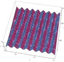
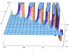
Figure 2: Plane Cosine wave $z=Cos(x-\sqrt{2}t)$ and Stable but de-attenuated irrational Cosine wave for $n=1$ in stretched variables with $\alpha=1/2,\ \beta=1/\sqrt{2}$ and $k=1$, $\omega_{p}=1$, $3<\tilde{v}^{2}>=1$.

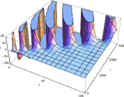
Figure 3: Unstable, attenuated irrational Cosine wave for $n=2$ in stretched variables with $\alpha=1/2,\ \beta=1/\sqrt{2}$ and $k=1$, $\omega_{p}=1$, $3<\tilde{v}^{2}>=1$.

To conclude this section, we note that turbulence is expected to set in much early in the present scenario compared to that from the conventional approach in an electrostatic plane electron wave.

3.2 Anomalous Transport

Our objective here is to study (charged) test (tracer) particles distribution within a model of the Vlasov plasma in the present dynamical scenario. As noted already, the Vlasov equation eq(10) is valid till the collective mode time scale $t$ is much smaller than the collision time scale $t_{c}$. In the above section we have seen that turbulence may set in even in a time scale $t\sim t_{c}^{a}<<t_{c}$ for a small multifractal exponent $0<a=a(\epsilon)<<1$. Recalling the fact that the collisionless equation (10) is nothing but the conservation of number density along a particle trajectory in the phase space i.e. $\frac{df}{dt}=0$, the onset of turbulence can also be associated with the loss of conservation of number density i.e. $\frac{df}{dt}\neq 0$ when $t\sim t_{c}^{a}$ mimicking collisional contributions from multifractal measures generated in the asymptotic boundary layer regions (c.f. eq(6) ).

Let us note next that with the onset of turbulence in, for example, the electrostatic model, the induced magnetic field fluctuations $\vec{B}$ need not be negligible, even in the simplified situation when one could continue to neglect the spontaneously enhanced collisional effects. The electrostatic model of Sec.3.1 now would be extended to the Vlasov-Maxwell equations (7) and (8). The test particle trajectory under the $\vec{E}\times\vec{B}$ drift wave limit is then given by

$$\frac{d\vec{x}}{dt}=\frac{1}{B^{2}}\vec{E}\times\vec{B}$$ (18)

Because of strong nonlinear coupling in the plasma model in presence of turbulence generating instabilities, a statistical treatment of this equation is considered appropriate. Any self-consistent solution of the plasma model would realize the electromagnetic field vectors $\vec{E}$ and $\vec{B}$ as random fluctuating fields, so that the tracer test particle equation (18) is interpreted as a stochastic Langevin equation.

As a specific simplified model, suppose the tracer particle travels initially in a steady electrostatic plasma fluid governed by the Vlasov-Poisson equation and $\vec{B_{0}}$ is a constant magnetic field along the $z$-axis, say. In a steady, stationary fluid profile, the tracer trajectory is likely to resemble a Brownian path, so that the underlying stochastic process driving the tracer particle equation (18) is Gaussian. The corresponding macroscopic description of this Brownian motion is given by the advection-diffusion (AVD) equation

$$\frac{\partial C}{\partial{t}}+{u}_{i}\frac{\partial C}{\partial{x}_{i}}={\frac{\partial}{\partial x_{i}}}{D\frac{\partial C}{\partial{x}_{i}}}$$ (19)

where $D$ is diffusivity and $C(x_{i},t)$ is the concentration density of an ensemble of tracer particles. Under the Markovian approximation $D=\underset{t\rightarrow\infty}{\lim}\frac{\sigma^{2}(t)}{2t}$ is approximately a constant leading to Gaussian scaling for the mean square deviation $\sigma^{2}(t)\sim 2Dt$.

Such a Gaussian scaling for particle trajectory however is expected for very short time evolution of the model. For a sufficiently large time i.e. when $t\sim T>>1$, we rewrite (19) by making use of its rescaling symmetry via the rescaled variables $\tilde{t}=\epsilon t$, $\tilde{x}_{i}=x_{i}/\xi(\epsilon),\ \epsilon^{-1}=T^{a}(\epsilon)\ 0<a(\epsilon)<<1$

$$\frac{\partial C}{\partial\tilde{t}}+\tilde{u}_{i}\frac{\partial C}{\partial\tilde{x}_{i}}=\nu\frac{\partial^{2}C}{\partial\tilde{x}_{i}^{2}}$$ (20)

where the rescaled diffusivity $\nu=D/\epsilon^{1+2h(\epsilon)}$ can become quite large when $\xi^{2}\sim\epsilon^{2h(\epsilon)},\ 0<h(\epsilon)<1/2$.

Next, we observe that the rescaled mean velocity of the fluid $\tilde{u}_{i}=\frac{d\tilde{x}^{i}}{d\tilde{t}}=\epsilon^{-(1-h)}u_{i}>>u_{i}$. The Reynolds number corresponding to the late time evolution of the plasma fluid would therefore be quite large, signaling once again the onset of turbulent inducing instabilities in the plasma fluid. The equation (20) would therefore represent the turbulent advection-diffusion equation. Although looks apparently Gaussian, the underlying motion in the rescaled variables is actually non-Gaussian, that we now establish.

We proceed in steps following the scenario presented in Sec.2:

1. We first recall that the rescaled variables actually denote nontrivial inversion induced transformations (c.f. Sec.2) in the late asymptotic limits $t\rightarrow\infty$ and $\epsilon\rightarrow 0^{+}$, in the sense that the boundary point $\tilde{t}=1$ is singular and unreachable; however the singularity is avoided by inversions of the form $\tilde{t}\mapsto{\tilde{t}}^{-1}=(\log\tilde{t})^{\alpha(\epsilon)},\ 0<\alpha(\epsilon)<1$, where $\tilde{t}$, in the r.h.s, lies close to 1, but exceeds 1.

2. Points 0 and $\infty$ of the positive real line are identified in a nontrivial manner under the above inversion. The asymptotic limit generates countable numbers of disconnected self similar sectors in the neighbourhoods of $\tilde{t}=0$ and $\tilde{t}=1$, with the identification of the right neighbourhood of $\tilde{t}=0$ of sector 1 with that of the right neighbourhood of $\tilde{t}=1$ of sector 2, and so on. The system of plasma (Vlasov-Maxwell, in the present case) equations are proliferated self similarly over each of the neighbourhoods. One particular example is presented in Sec.3.1 for the electrostatic model. As a hindsight, the neighbourhood of the origin of the physical coordinate space acquires a granular structure which in turn is mapped nontrivially to infinity by inversion. Physically, this mean that new sources of kinetic energy become available by inversion from the asymptotic boundary layers (c.f. final remarks in Sec.2).

3. At a macroscopic level such generation and proliferation of underlying plasma model over infinite number of disconnected (granular) asymptotic sectors would actually trigger formation of locally quasi-stable coherent structures (eddies etc.) leading to a new route to turbulence.

4. The asymptotic coherent structures shall produce effective (renormalized) multifractal measures, replacing the ordinary laminar state measures $dt$ and $dx_{i}$ respectively by the multifractal turbulent, but nevertheless, smooth measure $dt^{\alpha}$ and $dx_{i}^{\beta}$ where the multifractal exponents $\beta=\beta(\epsilon)>0$ and $\alpha=\alpha(\epsilon)>0$ respectively represent localized spatio-temporal scalings of asymptotic coherent structures (c.f. Sec.2).

5. For high Reynolds number $Re$, i.e. when $\nu\approx 0$ (equivalently very high mean velocity) the original laminar flow enters into a turbulent flow with a concomitant transformation of the laminar AVD equation (19) for passive tracers approximately into the turbulent AVD equation (20) involving asymptotic rescaled variables $\tilde{t}$ and $\tilde{x}_{i}$. In the asymptotic limits $t\rightarrow 1/\epsilon$, $\Delta x_{i}\rightarrow\xi(\epsilon)$ and $\epsilon\rightarrow 0$, the time and space variables are transformed into the smooth asymptotic multifractal scaling laws by inversion, viz; $d\tilde{t}\mapsto dT^{-1}=dt^{\alpha(\epsilon)},\ \alpha(\epsilon)>0$ and $d\tilde{x}_{i}\mapsto dX_{i}^{-1}=dx_{i}^{\beta(\epsilon)},\ \beta(\epsilon)>0$ as explained in Sec.2 (we assume, for simplicity, spatial homogeneity $\beta_{i}=\beta,\ \forall i$).

We recall that for a low Reynolds number (i.e. low mean speed) laminar flow increments and differential measures follow the standard Lebesgue measures of classical analysis. However, for higher Reynolds number flows tend to inhabit eddies of all possible length scales between the integral scale and the Kolmogorov’s molecular diffusion (dissipative) scale (i.e. between the largest and smallest eddy sizes). The turbulent AVD equation (20) is valid in the intermediate time $t_{I}<<t\sim 1/\epsilon$ and space $l_{K}<<x_{i}<<l_{I}$ scales where subscripts $K$ and $I$ denote appropriate Kolmogorov and integral scales respectively. Assuming that formation of eddies represent nonlinear structure formations in space and time dynamically, the nonlinear multifractal spatial increments as derived in Sec.2 provide a general framework of endowing a smooth, nevertheless, nonlinear measures on a multifractal fluid medium analogous to and paralleling the renormalization group analysis delivering a few finite measurable quantities in the form of scaling exponents even in the absence of a detailed microscopic theory of the given dynamical problem (i.e. the variation of tracer concentration in turbulent plasma flow). Here, the exponent $\beta$ denotes one of the scaling parameters derived from a general argument based on an inversion induced structure formation scenario bypassing a detailed theory of eddy formation and a specific model dependent derivation of nonlinear increments. One recently fashionable approach available in literature is the framework of fractional calculus. As remarked already, our approach is independent of fractional calculus techniques and as shown below can capture anomalous scaling of higher moments of tracer distribution quite naturally and easily. On the time domain, on the other hand, for a time scale greater than the integral scale $t_{I}$, the presence of infinitely large scales close to and beyond the time scale defined by the Reynolds number $t_{R}\sim Re\sim\nu^{-1}$, motion of a tracer particle will be enhanced indefinitely which will then contribute a small measurable renormalized quantity in the form of the nonlinear measure $dt^{\alpha},\ \alpha>0$ by inversion. For small positive values of $\alpha$ this nonlinear measure would model decelerated and/or sub-diffusive processes when $\alpha>1$ can lead to accelerated advection and/or super-diffusion.

Now, recognizing eq(20) as a standard AVD equation in the nonlinear deformed (stretched) variables $\tilde{t}=t^{\alpha(\epsilon)},t>0$ and $\tilde{x}=|x|^{\beta(\epsilon)}$, the concentration density with an initial delta pulse $C(x,0)=\delta(x)$ in a turbulent flow should have the generic form of the normal Gaussian distribution $C(x,t)=(\frac{1}{4\pi\kappa\tilde{t}})^{\frac{n}{2}}e^{-\frac{\tilde{X}^{2}}{4\nu\tilde{t}}}$ in the stretched variables $\tilde{t}$, $|\tilde{X}|$ where $X=x-Vt$. We remark that the definition of the stretched space variable $\tilde{X}$ takes care of the concomitant change in dimension of the corresponding stretched velocity vector $\tilde{V}$ so that $[\tilde{X}]=[\tilde{x}-\tilde{V}\tilde{t}]$. As a consequence the turbulent concentration density has finally the form of a heavy tailed stretched Gaussian (for definiteness, we consider only the one dimensional transport problem)

$$C(x,t)=t^{-\frac{\alpha(\epsilon)}{2}}G_{\beta(\epsilon)}(\frac{x-Vt}{t^{\alpha(\epsilon)/2\beta(\epsilon)}})$$ (21)

where the stretched Gaussian density is defined by [11, 13], $G_{\beta}(u)=\frac{1}{(4\pi\nu)^{\frac{1}{2}}}e^{-\frac{u^{2\beta}}{4\nu}}$. Using the substitution $u=\frac{x-Vt}{t^{\alpha/2\beta}}$, we now compute the mean and variance of the turbulent advected-diffusive transport in the form $<x>=\int_{-\infty}^{\infty}xC(x,t)dx=Vt^{1+\eta(\epsilon)}$ and $\sigma^{2}(t)=\int_{-\infty}^{\infty}(x-Vt)^{2}C(x,t)dx=(4\kappa)^{1/\beta(\epsilon)}t^{\gamma(\epsilon)}$, where $\eta(\epsilon)=\frac{\alpha(\epsilon)-\alpha(\epsilon)\beta(\epsilon)}{2\beta(\epsilon)}$ and $\gamma(\epsilon)=\frac{3\alpha(\epsilon)-\alpha(\epsilon)\beta(\epsilon)}{2\beta(\epsilon)}$. We note that the normal Gaussian statistics $\eta=0,\ \gamma=1$ characterizes the transport in a laminar flow. For turbulent transport one expects, on the other hand, anomalous non-Gaussian statistics. We have sub-advective and sub-diffusive behaviour for $\beta>1$ and $\alpha<2\beta(3-\beta)^{-1}$ (local dependence suppressed for simplicity of notation). The transport is super-advective and super-diffusive when $0<\beta<1$ and $\alpha>2\beta(3-\beta)^{-1}$. Incidentally, we note that the above anomalous scaling of the mean square displacement was also obtained by Chen et al [13] in the context of a fractal derivative diffusion problem. However, the definition of fractal derivative appears to be introduced in an ad hoc manner. The present approach might be considered to be a more rigorous independent derivation of the said scaling law.

The (multifractal) scaling exponents $\alpha$ and $\beta$ are free parameters to be fixed by matching the theoretical statistics $\eta$ and $\gamma$ with experimental data of a specific transport problem. The extrapolated values of $\alpha$ and $\beta$, in turn, should be important in distinguishing various physical characteristics of the turbulent flow and the associated transport problem. The actual problem of comparing the above analytical results with real data will be considered separately. We remark, however, that estimating scaling exponent $\alpha(\epsilon)$, for instance, would require evaluation of nonlinear jump increments of the form $\alpha(\epsilon)\approx\frac{\log\eta/\tilde{\eta}}{\log\eta/\epsilon}$ (c.f. Sec. 2.2) for linear increments $\eta=\Delta t$ and $\tilde{\eta}=\tilde{\Delta t}$ relative to the specified scale $\epsilon$ and satisfying $0<\tilde{\eta}<\epsilon<\eta$ from a time series data. It is expected that a log-log plot of the time series data from a turbulent flow would give a nontrivial slope $\alpha\neq 1$ for each choice of the scale $\epsilon$. This fact might be interpreted as an observational validation of the duality principle advocated in this paper.

4 Concluding Remarks

A new mechanism of instabilities and turbulence is discussed in the context of the kinetic Vlasov-Maxwell theory of plasma flow. The mechanism is based on a dynamic realization of extra kinetic energy influx from an asymptotic boundary layer region into the fluid flow. The production of extra kinetic energy is manifested in the form of multifractal measures indicating formation of multifractal granular structures in an unstable turbulent flow. The mathematical formalism that supports this copious production of multifractal structures is presented in detail. We illustrate the onset of new instability in the context of the warm plasma Langmuir wave dispersion relation. As a second example we show how the anomalous transport and a stretched Gaussian probability density function are derived from the turbulent advection-diffusion equation for a plasma flow in the present scenario. The comparison of the results presented here with experimental data will be considered elsewhere.

Acknowlegments

Authors thank the referee for insightful and constructive comments to improve the clarity and readability of the paper. Thanks are also due to A. Palit for help in drawing the figures.

REFERENCES

- [1] G. Consolini and T. Chang, Space Sci. Rev. 95, (2001), 309.
- [2] S.W.Y.Tam, T. Chang, P. M. Kinter and E. Klatt, Geophys. Res. Lett, 32, (2005), L05109.
- [3] B.A.Carreras, V.E.Lynch, D.E. Newman, R.Balbin, J.Bleuel, M.A.Pedrosa,M.Endler, B.v. Miligen, E.Senchez, C.Hidalgo, Phys. Plasma, 7(8), (2000), 3278.
- [4] C. Stan, C.P.Cristescu, D.G.Dimitriu, Rom. Journ. Phys. 56, (2011), 79.
- [5] B. Mandelbrot, The fractal geometry of Nature, Freeman, Sanfrancisco, (1984).
- [6] G. Parisi and U. Frisch, in Turbulence and predictibility in geophysical fluid dynamics and climate dynamics, North Holland, New York, (1985).
- [7] R. Benzi, G. Paladin, G.Parisi, A. Vulpiani, J.Phys.A:Math. Gen, 17, (1984), 3521.
- [8] U. Frish, Turbulence, Cambridge University Press, Cambridge, UK, (1995).
- [9] E Infeld, G Rowlands, Nonlinear waves, Solitons and Chaos, Cambrige University Press, Cambridge, (2000).
- [10] D. del-Castillo-Negrete, B. A. Carreras, and V. E. Lynch, Phys. Rev. Lett. 94, (2005), 065003.
- [11] R. Metzler, J Klafter, Phys. Rept. 339,(2000), 1-77.
- [12] V. E. Tarasov, J. Phys. A, 42, (2009), 465102.
- [13] W. Chen, H. Sun, X. Zhang, D. Korosak, Computers and Math. with Applications, 59,(2010), 1754.
- [14] K. Falconer, Fractal Geomtry: Mathematical Foundations and Application, John Wiley & Sons, England, (2000).
- [15] D. P. Datta, Radiation Effects and Defects in Solids, 166 (10), (2011), 757.
- [16] D. P. Datta, Radiation Effects and Defects in Solids, 167, (2013), 789.
- [17] D. P. Datta, Emergence of nonlinearity from novel scale invariance: applications to cosmology, (2013), Communicated.
- [18] D. P. Datta and S. Raut, Chaos, Solitons and Fractals, 28, (2006), 581.
- [19] S. Raut and D. P. Datta, Fractals, 18, (2010), 111.
- [20] D. P. Datta, S. Raut and A Raychaudhuri, p-Adic Numbers, Ultrametric Analysis and Applications, 3, (2011), 7.
- [21] M.-W. Ho, The Rainbow and the Worm: The Physics of Organisms (3rd Edition), World Scientific, Singapore, (2008).
- [22] N. D. Goldenfeld, O.Martin, and Y.Oono, J. Scient. Comput. 4, (1989), 355.