Towards $k$-connectivity of the random graph induced by a pairwise key predistribution scheme with unreliable links

Abstract

We study the secure and reliable connectivity of wireless sensor networks. Security is assumed to be ensured by the random pairwise key predistribution scheme of Chan, Perrig, and Song, and unreliable wireless links are represented by independent on/off channels. Modeling the network by an intersection of a random $K$-out graph and an Erdős-Rényi graph, we present scaling conditions (on the number of nodes, the scheme parameter $K$, and the probability of a wireless channel being on) such that the resulting graph contains no nodes with degree less than $k$ with high probability, when the number of nodes gets large. Results are given in the form of zero-one laws and are shown to improve the previous results by Yağan and Makowski on the absence of isolated nodes (i.e., absence of nodes with degree zero). Via simulations, the established zero-one laws are shown to hold also for the property of $k$-connectivity; i.e., the property that graph remains connected despite the deletion of any $k-1$ nodes or edges.

Keywords: Wireless Sensor Networks, Key Predistribution, Random Graphs, Minimum Node Degree, $k$-connectivity, Zero-one Laws.

1 Introduction

1.1 Motivation and Background

Wireless sensor networks (WSNs) are distributed collection of small sensor nodes that gather security-sensitive data and control security-critical operations in a wide range of industrial, home and business applications [1]. Many applications require deploying sensor nodes in hostile environments where an adversary can eavesdrop sensor communications, and can even capture a number of sensors and surreptitiously use them to compromise the network. Therefore, cryptographic protection is required to secure the sensor communication as well as to detect sensor capture and to revoke the compromised keys. Given the limited communication and computational resources available at each sensor, security is expected to be a key challenge in WSNs [6, 3, 14].

Random key predistribution is one of the approaches proposed in the literature for addressing security challenges in resource constrained WSNs. The idea of randomly assigning secure keys to the sensor nodes prior to network deployment was first introduced by Eschenauer and Gligor [6]. Following their original work, a large number of key predistribution schemes have been proposed; see the survey articles [14, 15] (and references therein).

Here we consider the random pairwise key predistribution scheme proposed by Chan et al. in [3]: Before deployment, each of the $n$ sensor nodes is paired (offline) with $K$ distinct nodes which are randomly selected from amongst all other nodes. For each sensor and any sensor paired to it, a unique (pairwise) key is generated and stored in their memory modules along with their ids. Two nodes can then secure an existing wireless communication link if at least one of them is paired to the other so that the two nodes have at least one pairwise key in common. Precise implementation details are given in Section 2.

Let $\mathbb{H}(n;K)$ denote the undirected random graph on the vertex set $\{1,\ldots,n\}$ where distinct nodes $i$ and $j$ are adjacent if they have a pairwise key in common as described earlier; this random graph models the random pairwise predistribution scheme under full visibility (whereby all nodes have a wireless link in between). The random graph $\mathbb{H}(n;K)$ is known in the literature on random graphs as the random $K$-out graph [2, 7, 8], and is typically defined in the following equivalent manner: For each of the $n$ vertices assign exactly $K$ arcs to $K$ distinct vertices that are selected uniformly at random, and then ignore the orientation of the arcs. Several properties of this graph have been recently analyzed by Yağan and Makowski [19, 20, 23, 22].

Recently, there has been a significant interest [10, 21, 17, 25, 24] to drop the full visibility assumption and to model and analyze random key predistribution schemes under more realistic situations that account for the possibility that communication links between nodes may not be available – This could occur due to the presence of physical barriers between nodes or because of harsh environmental conditions severely impairing transmission. With this in mind, several authors [21, 17, 25, 24] have started with a simple communication model where wireless links are represented by independent channels that are either on (with probability $p$) or off (with probability $1-p$). This suggests an overall modeling framework that is constructed by intersecting the random $K$-out graph $\mathbb{H}(n;K)$, with an Erdős-Rényi (ER) graph $\mathbb{G}(n;p)$ [2].

1.2 Contributions

In this paper, we initiate an analysis towards the $k$-connectivity for the resulting intersection graph $\mathbb{H\cap G}(n;K,p)$. A network (or graph) is said to be $k$-connected if its connectivity is preserved despite the failure of any $(k-1)$ nodes or links [11]. Therefore, the property of $k$-connectivity provides a guarantee of network reliability against the possible failures of sensors or links due to adversarial attacks or battery depletion; a much needed property given the key application areas of sensor networks such as health monitoring, battlefield surveillance, and environmental monitoring. Finally, $k$-connectivity has important benefits in mobile wireless sensor networks. For instance, if a network is known to be $k$-connected, then any $k-1$ nodes in the network are free to move anywhere in the network while the rest of the network remains at least 1-connected.

Our main result is a zero-one law for the property that the minimum node degree of $\mathbb{H\cap G}(n;K,p)$ is at least $k$. Namely, we present scaling conditions on the parameters $p$ and $K$ with respect to $n$, such that the resulting graph contains no nodes with degree less than $k$ with probability approaching to zero, or one, respectively, as the number of nodes $n$ gets large. The established results already imply the zero-law for the $k$-connectivity, since a graph can not be $k$-connected unless all nodes have degree at least $k$. Further, in most random graph models in the literature, including ER graphs, random geometric graphs [11], and random key graphs [24], the conditions that ensure $k$-connectivity coincide with those ensuring minimum node degree to be at least $k$. This is often established by showing the improbability of a graph being not $k$-connected when all nodes have at least $k$ neighbors. Here, we demonstrate this phenomenon via simulations which suggest that our zero-one laws hold also for the property of $k$-connectivity.

Furthermore, our results with $k=1$ constitute an improvement of the previous results by Yağan and Makowski [18, 21] on the absence of isolated nodes (i.e., absence of nodes with degree zero) in $\mathbb{H\cap G}(n;K,p)$. Namely, we show that the threshold for absence of isolated nodes (which is also the threshold for 1-connectivity) characterized in [18, 21] is not valid unless the limit $\lim_{n\to\infty}p_{n}\in[0,1]$ exists, a condition that was enforced throughout in [18, 21]. Instead, our main result indicates a new threshold function which does not require the existence of $\lim_{n\to\infty}p_{n}$. More importantly, we show that the new threshold function is stronger in that it indicates a sharper transition of the graph $\mathbb{H\cap G}(n;K,p)$ (as the parameters $K$ and $p$ increase) from having at least one isolated to having no isolated nodes almost surely; see Section 4.2 for details. We believe that the precise characterization of the threshold for absence of isolated will also pave the way to improving the results of [18, 21] for 1-connectivity of $\mathbb{H\cap G}(n;K,p)$.

Finally, our main contributions include a key confinement result that not only eases the proof of our main result, but is likely to play a key role in studying any monotone increasing property of the graph $\mathbb{H\cap G}(n;K_{n},p_{n})$; e.g., $k$-connectivity, existence of certain subgraphs, etc. In a nutshell, this confinement result shows that when seeking results for the asymptotic $k$-connectivity of $\mathbb{H\cap G}(n;K_{n},p_{n})$ with the parameters $K$ and $p$ scaled with number of nodes $n$, we can restrict our attention to a subclass of structured scalings (referred throughout as admissible scalings). In other words, we show that the aforementioned results (and others in the same vein) need only be established for such strongly admissible scalings. See Section 5.1 for details of the confinement argument, followed in Section 5.2 by its several useful consequences that arise in our context.

1.3 Notation and conventions

A word on the notation: All statements involving limits are understood with $n$ going to infinity. The random variables (rvs) under consideration are all defined on the same probability triple $(\Omega,{\cal F},\mathbb{P})$. Probabilistic statements are made with respect to this probability measure $\mathbb{P}$, and we denote the corresponding expectation operator by $\mathbb{E}$. The indicator function of an event $E$ is denoted by ${\bf 1}\left[E\right]$. Distributional equality is denoted by $=_{st}$. In comparing the asymptotic behaviors of the sequences $\{a_{n}\},\{b_{n}\}$, we use $a_{n}=o(b_{n})$, $a_{n}=O(b_{n})$, $a_{n}=\Omega(b_{n})$, and $a_{n}=\Theta(b_{n})$, with their meaning in the standard Landau notation. Namely, we write $a_{n}=o(b_{n})$ as a shorthand for the relation $\lim_{n\to\infty}\frac{a_{n}}{b_{n}}=0$, whereas $a_{n}=O(b_{n})$ means that there exists $c>0$ such that $a_{n}\leq cb_{n}$ for all $n$ sufficiently large. Also, we have $a_{n}=\Omega(b_{n})$ if $b_{n}=O(a_{n})$, or equivalently, if there exists $c>0$ such that $a_{n}\geq cb_{n}$ for all $n$ sufficiently large. Finally, we write $a_{n}=\Theta(b_{n})$ if we have $a_{n}=O(b_{n})$ and $a_{n}=\Omega(b_{n})$ at the same time.

1.4 Organization of the Paper

The paper is organized as follows: In Section 2, we give a formal model for the random pairwise key predistribution scheme of Chan et al., and introduce the induced random $K$-out graph. In particular, the main model $\mathbb{H\cap G}(n;K,p)$ considered in this paper, i.e., the intersection of a random $K$-out graph with an Erdős-Rényi graph, is introduced in Section 2.3. The main result of the paper concerning the minimum node degree of $\mathbb{H\cap G}(n;K,p)$ is presented in Section 3. In Section 4, we compare our results against the classical results of Erdős-Rényi and then against earlier results by Yağan and Makowski [21] on the absence of isolated nodes in $\mathbb{H\cap G}(n;K,p)$. Also in Section 4.3, we provide numerical results in support of our analytical results. The proof of the main result is initiated in Section 5 where we establish an important confining result that significantly eases the rest of the proof; there we also establish some preliminary scaling results to be used throughout. The proof of our main result is outlined in Section 6 and the necessary steps are established in Sections 7 through 11.

2 Model

2.1 The random pairwise key predistribution scheme

Interest in the random pairwise key predistribution scheme of Chan et al. [3] stems from the following advantages over the original Eschenauer - Gligor scheme: (i) Even if some nodes are captured, the secrecy of the remaining nodes is perfectly preserved; (ii) Unlike earlier schemes, this pairwise scheme enables both node-to-node authentication and quorum-based revocation. See also [16] for a detailed comparison of these two classical key predistribution schemes.

We parametrize the pairwise key distribution scheme by two positive integers $n$ and $K$ such that $K<n$. There are $n$ nodes, labelled $i=1,\ldots,n$, with unique ids ${\rm Id}_{1},\ldots,{\rm Id}_{n}$. Write ${\cal V}=\{1,\ldots,n\}$ and set ${\cal V}_{-i}={\mathcal{V}}-\{i\}$ for each $i=1,\ldots,n$. With node $i$, we associate a subset $\Gamma_{n,i}(K)$ of $K$ nodes selected uniformly at random from ${\cal V}_{-i}$, We say that each of the nodes in $\Gamma_{n,i}(K)$ is paired to node $i$. Thus, for any subset $A\subseteq{\cal V}_{-i}$, we require

$${\mathbb{P}}\left[{\Gamma_{n,i}(K)=A}\right]=\left\{\begin{array}[]{ll}{{n-1}\choose{K}}^{-1}&\mbox{if $|A|=K$}\\ &\\ 0&\mbox{otherwise.}\\ \end{array}\right.$$ (1)

Put differently, the selection of $\Gamma_{n,i}(K)$ is done uniformly amongst all subsets of ${\cal V}_{-i}$ which are of size $K$ and we further assume that rvs $\Gamma_{n,1}(K),\ldots,\Gamma_{n,n}(K)$ are mutually independent.

Once this offline random pairing has been created, we construct the key rings $\Sigma_{n,1}(K),\ldots,\Sigma_{n,n}(K)$, one for each node, as follows: Assumed available is a collection of $nK$ distinct cryptographic keys $\{\omega_{i|\ell},\ i=1,\ldots,n;\ \ell=1,\ldots,K\}$. Fix $i=1,\ldots,n$ and let $\ell_{n,i}:\Gamma_{n,i}(K)\rightarrow\{1,\ldots,K\}$ denote a labeling of $\Gamma_{n,i}(K)$. For each node $j$ in $\Gamma_{n,i}(K)$ paired to $i$, the cryptographic key $\omega_{i|\ell_{n,i}(j)}$ is associated with $j$. For instance, if the random set $\Gamma_{n,i}(K)$ is realized as $\{j_{1},\ldots,j_{K}\}$ with $1\leq j_{1}<\ldots<j_{K}\leq n$, then an obvious labeling consists in $\ell_{n,i}(j_{k})=k$ for each $k=1,\ldots,K$ so that key $\omega_{i|k}$ is associated with node $j_{k}$. Of course other labelings are possible. Finally, with node $j$ paired to node $i$, the pairwise key $\omega^{\star}_{n,ij}=[{\rm Id}_{i}|{\rm Id}_{j}|\omega_{i|\ell_{n,i}(j)}]$ is constructed and inserted in the memory modules of both nodes $i$ and $j$. The key $\omega^{\star}_{n,ij}$ is assigned exclusively to the pair of nodes $i$ and $j$, hence the terminology pairwise predistribution scheme. The key ring $\Sigma_{n,i}(K)$ of node $i$ is the set

$$\Sigma_{n,i}(K)=\left\{\omega^{\star}_{n,ij},\ j\in\Gamma_{n,i}(K)\right\}\cup\left\{\omega^{\star}_{n,ji},\ \begin{array}[]{c}j=1,\ldots,n\\ i\in\Gamma_{n,j}(K)\\ \end{array}\right\}$$ (4)

Two nodes $i$ and $j$, can secure an existing communication link if and only if $\Sigma_{n,i}(K)\cap\Sigma_{n,j}(K)\neq\emptyset$ which holds if at least one of the events $i\in\Gamma_{n,j}(K)$ or $j\in\Gamma_{n,i}(K)$ takes place. Namely, it is plain that

$$[\Sigma_{n,i}(K)\cap\Sigma_{n,j}(K)\neq\emptyset]=[i\in\Gamma_{n,j}(K)]\cup[j\in\Gamma_{n,i}(K)]$$

Both events can take place, in which case the memory modules of node $i$ and $j$ both contain the distinct keys $\omega^{\star}_{n,ij}$ and $\omega^{\star}_{n,ji}$. It is plain by construction that this scheme supports distributed node-to-node authentication.

2.2 Random $K$-out graphs

The pairwise key predistribution scheme naturally gives rise to the following class of random graphs: With $n=2,3,\ldots$ and positive integer $K<n$, we say that the distinct nodes $i$ and $j$ are K-adjacent, written $i\sim_{K}j$, if and only if they have at least one key in common in their key rings, namely

$$i\sim_{K}j\quad\mbox{iff}\quad\Sigma_{n,i}(K)\cap\Sigma_{n,j}(K)\neq\emptyset.$$ (5)

Let $\mathbb{H}(n;K)$ denote the undirected random graph on the vertex set $\{1,\ldots,n\}$ induced by the adjacency notion (5). This ensures that edges in $\mathbb{H}(n;K)$ represent pairs of sensors that have at least one cryptographic key in common, and thus that can securely communicate over an existing communication channel. Let $\lambda_{n}(K)$ define the edge assignment probability in $\mathbb{H}(n;K)$; i.e., we have

$${\mathbb{P}}\left[{i\sim_{K}j}\right]=\lambda_{n}(K)$$ (6)

for any distinct $i,j\in\mathcal{V}$. It is easy to check that

$$\lambda_{n}(K)=1-{\mathbb{P}}\left[{i\not\in\Gamma_{n,j}(K)~{}\cap~{}j\not\in\Gamma_{n,i}(K)}\right]=1-\left(\frac{{{n-2}\choose{K}}}{{{n-1}\choose{K}}}\right)^{2}=\frac{2K}{n-1}-\left(\frac{K}{n-1}\right)^{2}.$$ (7)

The random graph $\mathbb{H}(n;K)$ is known in the literature on random graphs as the random $K$-out graph [2, 8], or random $K$-orientable graph [7]. Those references adopt the following definition, which can easily be seen to be equivalent to the adjacency condition (5): For each of the $n$ vertices assign exactly $K$ arcs to $K$ distinct vertices that are selected uniformly at random, and then ignore the orientation of the arcs. The directed version of this graph (i.e., with the orientation of the arcs preserved) has also been studied; e.g., see the work by Philips et al. [12], who showed that the diameter of the directed $K$-out graph concentrates almost surely on two values.

2.3 Intersection of random graphs

As mentioned earlier, we assume a simple wireless communication model that consists of independent channels, each of which can be either on or off. Thus, with $p$ in $(0,1)$, let $\{B_{ij}(p),1\leq i<j\leq n\}$ denote i.i.d. $\{0,1\}$-valued rvs with success probability $p$. The channel between nodes $i$ and $j$ is available (resp. up) with probability $p$ and unavailable (resp. down) with the complementary probability $1-p$.

Distinct nodes $i$ and $j$ are said to be B-adjacent, written $i\sim_{B}j$, if $B_{ij}(p)=1$. B-adjacency defines the standard Erdős-Rényi (ER) graph $\mathbb{G}(n;p)$ on the vertex set $\{1,\ldots,n\}$ [2]. Obviously, ${\mathbb{P}}\left[{i\sim_{B}j}\right]=p.$

The random graph model studied here is obtained by intersecting the random graphs induced by the pairwise key predistribution scheme, and by the on-off communication model, respectively. Namely, we consider the intersection of $\mathbb{H}(n;K)$ with the ER graph $\mathbb{G}(n;p)$. In this case, distinct nodes $i$ and $j$ are said to be adjacent, written $i\sim j$, if and only they are both K-adjacent and B-adjacent, namely

$$i\sim j~{}~{}\quad\mbox{iff}~{}~{}~{}\quad\Sigma_{n,i}(K)\cap\Sigma_{n,j}(K)\neq\emptyset~{}~{}\mbox{and}~{}~{}B_{ij}(p)=1.$$ (8)

The resulting undirected random graph defined on the vertex set $\{1,\ldots,n\}$ through this notion of adjacency is denoted $\mathbb{H\cap G}(n;K,p)$. The relevance of $\mathbb{H\cap G}(n;K,p)$ in the context of secure WSNs is now clear. Two nodes that are connected by an edge in $\mathbb{H\cap G}(n;K,p)$ share at least one cryptographic key and have a wireless link available to them, so that they can establish a secure communication link.

Throughout we assume the collections of rvs $\{\Gamma_{n,1}(K),\ldots,\Gamma_{n,n}(K)\}$ and $\{B_{ij}(p),1\leq i<j\leq n\}$ to be independent, in which case the edge occurrence probability in $\mathbb{H\cap G}(n;K,p)$ is given by

$${\mathbb{P}}\left[{i\sim j}\right]={\mathbb{P}}\left[{i\sim_{K}j}\right]{\mathbb{P}}\left[{i\sim_{B}j}\right]=p\lambda_{n}(K).$$ (9)

3 The result

Our main technical result is given next. To fix the terminology, we refer to any mapping $K:\mathbb{N}_{0}\rightarrow\mathbb{N}_{0}$ as a scaling (for random $K$-out graphs) provided it satisfies the natural conditions

$$K_{n}<n\qquad n=1,2,\ldots.$$ (10)

Similarly, we let any mapping $p:\mathbb{N}_{0}\rightarrow[0,1]$ define a scaling for Erdős-Rényi graphs.

To lighten the notation we often group the parameters $K$ and $p$ into the ordered pair $\theta\equiv(K,p)$. Hence, a mapping $\theta:\mathbb{N}_{0}\rightarrow\mathbb{N}_{0}\times[0,1]$ defines a scaling for the intersection graph $\mathbb{H\cap G}(n;\theta)$ provided that the condition (10) holds.

Theorem 3.1

Consider scalings $K:\mathbb{N}_{0}\rightarrow\mathbb{N}_{0}$ and $p:\mathbb{N}_{0}\rightarrow[0,1]$ such that $\lim_{n\to\infty}(n-2K_{n})=\infty$ and $\limsup_{n\to\infty}p_{n}<1$. With the sequence $\gamma:\mathbb{N}_{0}\rightarrow\mathbb{R}$ defined through

$$p_{n}K_{n}\left(1-\frac{\log(1-p_{n})}{p_{n}}-\frac{K_{n}}{n-1}\right)=\log n+(k-1)\log\log n+\gamma_{n}$$ (11)

we have

$$\lim_{n\rightarrow\infty}{\mathbb{P}}\left[{\textrm{Min~{}node~{}degree~{}of~{}}\atop\mathbb{H}\cap\mathbb{G}(n;\theta_{n})~{}\textrm{ is~{}no~{}less~{}than~{}}k}\right]=\left\{\begin{array}[]{ll}0&\mbox{{if}~{} $\lim\limits_{n\to\infty}\gamma_{n}=-\infty$}\\ &\\ 1&\mbox{{if} ~{}$\lim\limits_{n\to\infty}\gamma_{n}=+\infty$}.\end{array}\right.$$ (15)

The proof of Theorem 3.1 passes through the method of first and second moments [8], applied to the random variable counting the number of nodes with degree $\ell$, with $\ell=0,1,\ldots,k-1$. Although this technique is standard in the literature, its application to the intersection graph $\mathbb{H\cap G}(n;\theta)$ is far from being straightforward due to intricate dependencies amongst the degrees of nodes. The proof of Theorem 3.1 is given in Sections 6 through 11.

The extra conditions enforced by Theorem 3.1 are required for technical reasons; i.e., for the method of moments to be applied successfully to the aforementioned count variables. However, we remark that these conditions are mild and do not preclude their application in realistic WSN scenarios. First, the condition $\limsup_{n\to\infty}p_{n}<1$ enforces that wireless communication channels between nodes do not become available with probability one as $n$ gets large. The situation $\limsup_{n\to\infty}p_{n}=1$ that is not covered by our result is reminiscent of the full visibility case considered in [22], and is not likely to hold in practice. In fact, as the number of nodes gets large, it may be expected that $p_{n}$ goes to zero due to interference associated with a large number of nodes communicating simultaneously. Second, the condition $\lim_{n\to\infty}(n-2K_{n})=\infty$ will already follow if $2K_{n}\leq cn$ for some $c<1$. Given that $2K_{n}$ is equal to the mean number of keys stored per sensor in the pairwise scheme [23], this condition needs to hold in any practical WSN scenario due to limited memory and computational capability of the sensors. In fact, Di Pietro et al. [4] noted that key ring sizes on the order of $\log n$ are feasible for WSNs.

We now present a simple corollary of Theorem 3.1, that will help in comparing our main result with the classical results of Erdős-Rényi [5].

Corollary 3.2

Consider scalings $K:\mathbb{N}_{0}\rightarrow\mathbb{N}_{0}$ and $p:\mathbb{N}_{0}\rightarrow[0,1]$ such that $\lim_{n\to\infty}(n-2K_{n})=\infty$ and $\limsup_{n\to\infty}p_{n}<1$. With the sequence $\gamma:\mathbb{N}_{0}\rightarrow\mathbb{R}$ defined through

$$\frac{p_{n}K_{n}}{n-1}\left(1-\frac{\log(1-p_{n})}{p_{n}}-\frac{K_{n}}{n-1}\right)=\frac{\log n+(k-1)\log\log n+\gamma_{n}}{n}$$ (16)

we have

$$\lim_{n\rightarrow\infty}{\mathbb{P}}\left[{\textrm{Min~{}node~{}degree~{}of~{}}\atop\mathbb{H}\cap\mathbb{G}(n;\theta_{n})~{}\textrm{ is~{}no~{}less~{}than~{}}k}\right]=\left\{\begin{array}[]{ll}0&\mbox{{if}~{} $\lim\limits_{n\to\infty}\gamma_{n}=-\infty$}\\ &\\ 1&\mbox{{if} ~{}$\lim\limits_{n\to\infty}\gamma_{n}=+\infty$}.\end{array}\right.$$ (20)

Proof.  Pick scalings $K:\mathbb{N}_{0}\rightarrow\mathbb{N}_{0}$ and $p:\mathbb{N}_{0}\rightarrow[0,1]$ such that $\lim_{n\to\infty}(n-2K_{n})=\infty$ and $\limsup_{n\to\infty}p_{n}<1$. Define the sequence $\gamma:\mathbb{N}_{0}\rightarrow\mathbb{R}$ through (11). For this scaling, we have

$$\frac{p_{n}K_{n}}{n-1}\left(1-\frac{\log(1-p_{n})}{p_{n}}-\frac{K_{n}}{n-1}\right) = \frac{\log n+(k-1)\log\log n+\gamma_{n}}{n-1}$$ (21)

$$= \frac{\log n+(k-1)\log\log n+\gamma_{n}+\frac{\log n+(k-1)\log\log n+\gamma_{n}}{n-1}}{n}$$

$$= \frac{\log n+(k-1)\log\log n+\gamma_{n}(1+o(1))+o(1)}{n}.$$

Comparing (21) with (16), we get the desired result (20) from (15) as we note that

$$\lim_{n\to\infty}\gamma_{n} = +\infty\qquad\textrm{if and only if}\qquad\lim_{n\to\infty}\left(\gamma_{n}(1+o(1))+o(1)\right)=+\infty$$

$$\lim_{n\to\infty}\gamma_{n} = -\infty\qquad\textrm{if and only if}\qquad\lim_{n\to\infty}\left(\gamma_{n}(1+o(1))+o(1)\right)=-\infty.$$

 

4 Comments and Discussion

4.1 Comparison with Erdős-Rényi Graphs

For each $p$ in $[0,1]$ and $n=2,3,\ldots$, let $\mathbb{G}(n;p)$ denote the Erdős-Rényi graph on the vertex set $\{1,\ldots,n\}$ with edge probability $p$. It is known that edge assignments are mutually independent in $\mathbb{G}(n;p)$, whereas they are strongly correlated in $\mathbb{H}(n;K)$ in that they are negatively associated in the sense of Joag-Dev and Proschan [9]; see [21] for details. Thus, $\mathbb{H}(n;K)$ cannot be equated with $\mathbb{G}(n;p)$ even when the parameters $p$ and $K$ are selected so that the edge assignment probabilities in these two graphs coincide, say $\lambda(n;K)=p$. Therefore, $\mathbb{H\cap G}(n;\theta)$ cannot be equated with an ER graph either, and the results obtained here are not mere consequences of classical results for ER graphs.

However, some similarities do exist between $\mathbb{H\cap G}(n;\theta)$ and ER graphs. We start by presenting the following well-known zero-one law for $k$-connectivity in ER graphs [5]: For any scaling $p:\mathbb{N}_{0}\rightarrow[0,1]$ satisfying

$$p_{n}=\frac{\log n+(k-1)\log\log n+\gamma_{n}}{n}$$ (22)

for some $\gamma:\mathbb{N}_{0}\to\mathbb{R}$, it holds that

$$\lim_{n\rightarrow\infty}{\mathbb{P}}\left[{~{}\mathbb{G}(n;p_{n})\mbox{~{}is $k$-connected~{}}}\right]$$ (26)

$$= \lim_{n\rightarrow\infty}{\mathbb{P}}\left[{~{}\mathbb{G}(n;p_{n})\mbox{~{}has min. node degree $\geq k$~{}}}\right]=\left\{\begin{array}[]{ll}0&\mbox{if~{} $\gamma_{n}\to-\infty$}\\ &\\ 1&\mbox{if~{} $\gamma_{n}\to+\infty$.}\end{array}\right.$$

We now compare this with our main result by means of Corollary 3.2. Notice that the right-hand sides of the scalings (16) and (22) are exactly the same, and so are the corresponding zero-one laws (20) and (26), respectively. In the case of the ER graph $\mathbb{G}(n;p_{n})$, the left-hand side of (22) corresponds to the edge probability $p_{n}$. We now explore how the left-hand side of (16) is related to the corresponding edge probability $p_{n}\lambda_{n}(K_{n})$ (viz. (9)) of the graph $\mathbb{H}\cap\mathbb{G}(n;\theta_{n})$. First, we recall (7) and use the fact that $\log(1-p_{n})\leq-p_{n}$ to get

$$\frac{p_{n}K_{n}}{n-1}\left(1-\frac{\log(1-p_{n})}{p_{n}}-\frac{K_{n}}{n-1}\right)\geq p_{n}\lambda_{n}(K_{n}).$$

Hence, in ER graphs the threshold of $k$-connectivity, and of minimum node degree being at least $k$, appears when the link probability is compared against $(\log n+(k-1)\log\log n)/n$. In $\mathbb{H\cap G}(n;\theta_{n})$, our result shows that the threshold appears when a quantity that is always larger than the link probability $p_{n}\lambda_{n}(K_{n})$ is compared against $(\log n+(k-1)\log\log n)/n$. This indicates that $\mathbb{H\cap G}(n;\theta_{n})$ tends to exhibit the property that all nodes have at least $k$ neighbors easier than ER graphs; i.e., this property can be ensured by a smaller link probability between nodes (which leads to smaller average node degree).

The situation is more intricate if it holds that $\lim_{n\to\infty}p_{n}=0$, whence we have

$$\log(1-p_{n})=-p_{n}-\frac{p_{n}^{2}}{2}(1+o(1)).$$

This leads to

$$\frac{p_{n}K_{n}}{n-1}\left(1-\frac{\log(1-p_{n})}{p_{n}}-\frac{K_{n}}{n-1}\right) = \frac{p_{n}K_{n}}{n-1}\left(2-\frac{K_{n}}{n-1}+\frac{p_{n}}{2}(1+o(1))\right)\qquad\qquad\qquad\qquad$$ (27)

$$= \frac{p_{n}K_{n}}{n-1}\left(2-\frac{K_{n}}{n-1}\right)\left(1+\frac{p_{n}}{2}\cdot\frac{1+o(1)}{2-\frac{K_{n}}{n-1}}\right)$$

$$= p_{n}\lambda_{n}(K_{n})(1+\Theta(p_{n}))$$

$$= p_{n}\lambda_{n}(K_{n})(1+o(1)),$$ (28)

where in (27), we used the fact that $1\leq 2-\frac{K_{n}}{n-1}\leq 2$ since $K_{n}\leq n-1$. Thus, in the practically relevant case when the wireless channels become weaker as $n$ gets large, the threshold for minimum node degree of $\mathbb{H\cap G}(n;\theta_{n})$ to be at least $k$ appears when a quantity that is asymptotically equivalent to link probability is compared against $(\log n+(k-1)\log\log n)/n$; a situation that is reminiscent of the ER graphs. A similar observation was made in [21] for the threshold of $1$-connectivity and absence of isolated nodes.

Nevertheless, it is worth mentioning that even under $\lim_{n\to\infty}p_{n}=0$, the zero-one laws for the minimum node degree being at least $k$ in ER graphs and $\mathbb{H\cap G}(n;\theta_{n})$ are not exactly analogous. This is because, the term $o(1)$ in (28) may change the behavior of the sequence $\gamma_{n}$ appearing in (16) as it is given by

$$\gamma_{n} = np_{n}\lambda_{n}(K_{n})(1+\Theta(p_{n}))-\log n-(k-1)\log\log n$$

$$= np_{n}\lambda_{n}(K_{n})-\log n-(k-1)\log\log n+\Theta(np_{n}^{2}\lambda_{n}(K_{n}))$$

$$= np_{n}\lambda_{n}(K_{n})-\log n-(k-1)\log\log n+\Theta(K_{n}p_{n}^{2})$$

as we note that $\lambda_{n}(K_{n})=\Theta(K_{n}/n)$. It is now clear that, even under $\lim_{n\to\infty}p_{n}=0$, the two results, (26) under (22) and (20) under (16), may be deemed analogous if and only if $K_{n}p_{n}^{2}$ is bounded, i.e., $K_{n}p_{n}^{2}=O(1)$. Combining, we can conclude that for the two graphs, $\mathbb{G}(n;p_{n})$ and $\mathbb{H\cap G}(n;K_{n},p_{n})$, to exhibit asymptotically the same behavior for the property that their minimum node degrees are at least $k$, the parameter scalings should satisfy

$$p_{n}=o(1)\qquad\textrm{and}\qquad K_{n}p_{n}^{2}=O(1).$$

4.2 Comparison with results by Yağan and Makowski for $k=1$

We now compare our results with those by Yağan and Makowski [21] who established zero-one laws for 1-connectivity, and for the absence of isolated nodes (i.e., absence of nodes with degree zero) in $\mathbb{H\cap G}(n;\theta)$. Here, we present their result in a slightly different form: Consider scalings $K:\mathbb{N}_{0}\rightarrow\mathbb{N}_{0}$ and $p:\mathbb{N}_{0}\rightarrow(0,1)$ such that

$$p_{n}K_{n}\left(2-\frac{K_{n}}{n-1}\right)\left(\frac{1-\frac{\log(1-p_{n})}{p_{n}}}{2}\right)\sim c\log n,$$ (29)

for some $c>0$. Assume also that $\lim_{n\to\infty}p_{n}=p^{\star}$ exists. Then, we have

$$\lim_{n\rightarrow\infty}{\mathbb{P}}\left[{\mathbb{H\cap G}(n;\theta_{n})~{}\mbox{is connected}}\right]$$ (33)

$$= \lim_{n\rightarrow\infty}{\mathbb{P}}\left[{\mathbb{H\cap G}(n;\theta_{n})~{}\mbox{contains~{}no~{}isolated~{}nodes }}\right]=\left\{\begin{array}[]{ll}0&\mbox{if~{} $c<1$}\\ &\\ 1&\mbox{if~{} $c>1$}.\end{array}\right.$$

To better compare this result with ours, we set $k=1$ and rewrite our scaling condition (11) as

$$p_{n}K_{n}\left(2-\frac{K_{n}}{n-1}\right)\left(\frac{1-\frac{\log(1-p_{n})}{p_{n}}-\frac{K_{n}}{n-1}}{2-\frac{K_{n}}{n-1}}\right)=\log n+\gamma_{n}$$ (34)

under which Theorem 3.1 gives

$$\lim_{n\rightarrow\infty}{\mathbb{P}}\left[{\mathbb{H}\cap\mathbb{G}(n;\theta_{n})~{}\atop{\textrm{ has~{}no~{}isolated~{}nodes~{}}}}\right]=\left\{\begin{array}[]{ll}0&\mbox{{if}~{} $\gamma_{n}\to-\infty$}\\ &\\ 1&\mbox{{if} ~{}$\gamma_{n}\to+\infty$}.\end{array}\right.$$ (38)

We now argue how our result on absence of isolated nodes constitutes an improvement on the result of [21]. The assumption that limit $\lim_{n\to\infty}p_{n}=p^{\star}$ exists was the key in establishing (33) under (29) and our results in this paper explains why. First, it is clear that if $p^{\star}=0$, then

$$\lim_{n\to\infty}\left(\frac{1-\frac{\log(1-p_{n})}{p_{n}}}{2}\right)=1=\lim_{n\to\infty}\left(\frac{1-\frac{\log(1-p_{n})}{p_{n}}-\frac{K_{n}}{n-1}}{2-\frac{K_{n}}{n-1}}\right)$$

so that the left hand sides of (34) and (29) are asymptotically equivalent. Next, if $p^{\star}>0$, then it follows that $K_{n}=O(\log n)$ (see [21]) under (29). This again yields the asymptotical equivalence of the left hand sides of (34) and (29). Therefore, under the assumption that $p_{n}$ has a limit, a scaling condition that is equivalent to (29) is given by

$$p_{n}K_{n}\left(2-\frac{K_{n}}{n-1}\right)\left(\frac{1-\frac{\log(1-p_{n})}{p_{n}}-\frac{K_{n}}{n-1}}{2-\frac{K_{n}}{n-1}}\right)\sim c\log n,$$ (39)

with the results (33) unchanged.

Comparing (34) with (39), we see that our absence of isolated nodes result is more fine-grained than the one given in [21]. In a nutshell, the scaling condition (39) enforced in [21] requires a deviation of $\gamma_{n}=\pm\Omega(\log n)$ (from the threshold $\log n$) to get the zero-one law, whereas in our formulation (34), it suffices to have an unbounded deviation; e.g., even $\gamma_{n}=\pm\log\log\cdots\log n$ will do. Put differently, we cover the case of $c=1$ in (33) under (39) and show that $\mathbb{H\cap G}(n;\theta_{n})$ could be almost surely free of or not free of isolated nodes, depending on the limit of ${\gamma_{n}}$; in fact, if (39) holds with $c>1$, we see from Theorem 3.1 that $\mathbb{H\cap G}(n;\theta_{n})$ is not only free of isolated nodes but also all of its nodes will have degree larger than $k$ for all $k=1,2,\ldots$.

4.3 Numerical results and a conjecture

We now present some numerical results to check the validity of Theorem 3.1, particularly in the non-asymptotic regime, i.e., when parameter values are set in accordance with real-world wireless sensor network scenarios. In all experiments, we fix the number of nodes at $n=2000$. Then for a given parameter pair $(K,p)$, we generate $200$ independent samples of the graph $\mathbb{H\cap G}(n;K,p)$ and count the number of times (out of a possible 200) that the obtained graphs i) have minimum node degree no less than $k$ and ii) are $k$-connected, for $k=1,2,\ldots$. Dividing the counts by $200$, we obtain the (empirical) probabilities for the events of interest.

In Figure 1, we depict the resulting empirical probability that each node in $\mathbb{H\cap G}(n;K,p)$ has degree at least $2$ as a function of $K$ for various $p$ values. For each $p$ value, we also show the critical threshold of having minimum degree at least $2$ asserted by Theorem 3.1 (viz. (11)) by a vertical dashed line. Namely, the vertical dashed lines stand for the minimum integer value of $K$ that satisfies

$$pK\left(1-\frac{\log(1-p)}{p}-\frac{K}{n-1}\right)>\log n+\log\log n$$ (40)

Even with $n=2000$, we can observe the threshold behavior suggested by Theorem 3.1; i.e., the probability that $\mathbb{H\cap G}(n;K,p)$ has minimum node degree at least $k$ transitions from zero to one as $K$ varies very slightly from a certain value. Those $K$ values match well the vertical dashed lines suggested by Theorem 3.1, leading to the conclusion that numerical experiments are in good agreement with our theoretical results.

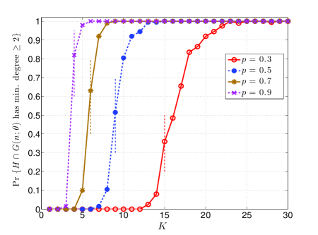
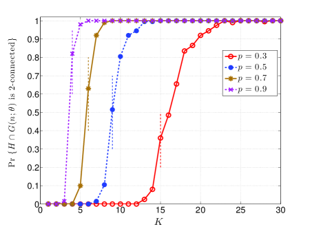
Figure 1: a) Probability that all nodes in $\mathbb{H}\cap\mathbb{G}(n;K,p)$ have degree at least 2 as a function of $K$ for $p=0.3$, $p=0.5$, $p=0.7$, and $p=0.9$ with $n=2000$. b) Probability that $\mathbb{H}\cap\mathbb{G}(n;K,p)$ is 2-connected as a function of $K$ for $p=0.3$, $p=0.5$, $p=0.7$, and $p=0.9$ with $n=2000$. The two figures being indistinguishable suggests that an analog of Theorem 3.1 holds also for the property of $k$-connectivity.

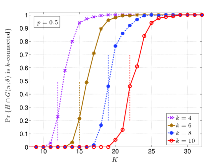
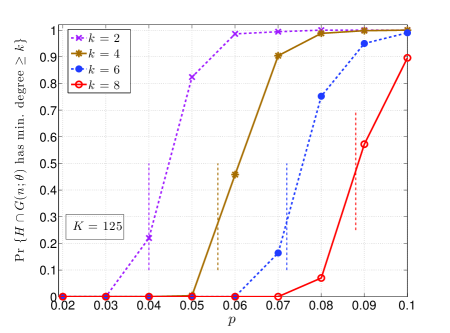
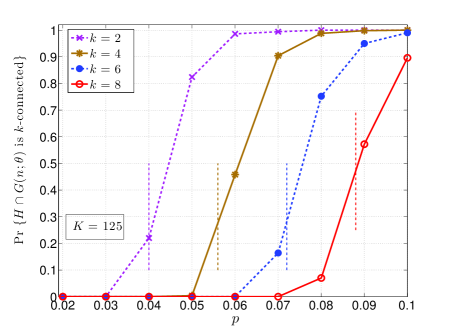
Figure 2: a,b) With $n=2000$ and $p=0.5$, the probability that all nodes in $\mathbb{H}\cap\mathbb{G}(n;K,p)$ have degree at least $k$, and the probability that $\mathbb{H}\cap\mathbb{G}(n;K,p)$ is $k$-connected are plotted, respectively, as a function of $K$. c,d) With $n=2000$ and $K=125$, the probability that all nodes in $\mathbb{H}\cap\mathbb{G}(n;K,p)$ have degree at least $k$, and the probability that $\mathbb{H}\cap\mathbb{G}(n;K,p)$ is $k$-connected are plotted, respectively as a function of $p$.

Figure 1 is obtained in the same way with Figure 1, this time for the probability that $\mathbb{H\cap G}(n;K,p)$ is $2$-connected. It is clear that two figures show a strong similarity with curves corresponding to each $p$ value being almost indistinguishable. This raises the possibility that an analog of the zero-one law given in Theorem 3.1 holds also for the property of $k$-connectivity in $\mathbb{H}\cap\mathbb{G}(n;K,P)$. This would be reminiscent of several other random graph models from the literature where the two graph properties (min. node degree $\geq k$ and $k$-connectivity) shown to be asymptotically equivalent; e.g., see ER graphs [5] (viz. (26)), random key graphs and their intersection with ER graphs [13, 24], and random geometric graphs over a unit torus [11].

To drive this point further, we have conducted an extensive simulation study and compared the empirical probabilities for the properties of minimum node degree is at least $k$, and $k$-connectivity in graph $\mathbb{H}\cap\mathbb{G}(n;K,P)$. Some of the results are reported in Figures 2-2, and they strongly suggest the equivalence of these two properties in $\mathbb{H}\cap\mathbb{G}(n;K,P)$ as well. This leads us to cast the following conjecture, which is the analog of Theorem 3.1 for $k$-connectivity.

Conjecture 4.1

Consider scalings $K:\mathbb{N}_{0}\rightarrow\mathbb{N}_{0}$ and $p:\mathbb{N}_{0}\rightarrow[0,1]$ such that $\lim_{n\to\infty}(n-2K_{n})=\infty$ and $\limsup_{n\to\infty}p_{n}<1$, and a sequence $\gamma:\mathbb{N}_{0}\rightarrow\mathbb{R}$ defined through (11). Then,

$$\lim_{n\rightarrow\infty}{\mathbb{P}}\left[{\mathbb{H}\cap\mathbb{G}(n;\theta_{n})~{}\textrm{is $k$-connected}}\right]=\left\{\begin{array}[]{ll}0&\mbox{{if}~{} $\gamma_{n}\to-\infty$}\\ &\\ 1&\mbox{{if} ~{}$\gamma_{n}\to+\infty$}.\end{array}\right.$$ (44)

We close this section with a few comments on Conjecture 4.1, before we start the proof of our main result in the next section. First, it is clear that if a graph has minimum node degree less than $k$, i.e., it has at least one vertex whose degree is less than or equal to $k-1$, then it will be not $k$-connected. This is because the graph can be made disconnected by taking all the neighbors of the node with degree $\leq k-1$; i.e., by taking less than or equal to $k-1$ nodes. Therefore, Theorem 3.1 already establishes the zero-law of the Conjecture 4.1. Namely, it is clear under the enforced assumptions on the scalings that

$$\lim_{n\rightarrow\infty}{\mathbb{P}}\left[{\mathbb{H}\cap\mathbb{G}(n;\theta_{n})~{}\textrm{is $k$-connected}}\right]=0\qquad\textrm{if}\quad\gamma_{n}\to-\infty.$$

Therefore, it only remains to establish the one-law in Conjecture 4.1. In view of Theorem 3.1, this will follow if it is shown that

$$\lim_{n\rightarrow\infty}{\mathbb{P}}\left[{\mathbb{H}\cap\mathbb{G}(n;\theta_{n})~{}\textrm{is {\em not} $k$-connected}~{}\bigcap~{}\atop~{}~{}~{}\mathbb{H}\cap\mathbb{G}(n;\theta_{n})~{}\textrm{has min.~{}degree $\geq k$}}\right]=0\qquad\textrm{if}\quad\gamma_{n}\to+\infty.$$ (45)

Exploring the validity of (45) is one of the main directions to be followed in the future work.

5 Preliminaries

Before we give a proof of Theorem 3.1, we collect in this section some preliminary results that will be used throughout.

5.1 A reduction step: Confining $\gamma_{n}$

A key step in proving Theorem 3.1 is to restrict the deviation function $\gamma_{n}$ defined through (11) to satisfy $\gamma_{n}=\pm o(\log n)$; i.e., that

$$\lim_{n\to\infty}\frac{\gamma_{n}}{\log n}=0.$$ (46)

Some useful consequences of (46) are established in Section 5.2. In this section, we will show that (46) can be assumed without loss of generality in establishing Theorem 3.1. More precisely, we will show that

Theorem 3.1 under $$\gamma_{n}=\pm o(\ln n) \Rightarrow$$ Theorem 3.1 (47)

First, we establish the fact that $\gamma_{n}$ defined through (11) is monotone increasing in both parameters $p_{n}$ and $K_{n}$.

Proposition 5.1

With $p$ in $(0,1)$ and a positive integer $K<n$, the function

$$\gamma_{n}=pK\left(1-\frac{\log(1-p)}{p}-\frac{K}{n-1}\right)-\log n-(k-1)\log\log n$$ (48)

is monotone increasing in $p$ and $K$.

Proof.  We first show that $\gamma_{n}$ is monotone increasing in $p$. Taking the derivative of (48) with respect to $p$, we get

$$\frac{d}{dp}\gamma_{n} = \frac{d}{dp}\left(pK-K\log(1-p)-p\frac{K^{2}}{n-1}\right)$$

$$= K+K\frac{1}{1-p}-\frac{K^{2}}{n-1}$$

$$\geq K+K\frac{1}{1-p}-K$$

$$\geq 0,$$

where, in (5.1) we used the fact that $K\leq n-1$.

Next, we show that $\gamma_{n}$ is monotone increasing in $K$ as well. To see this, take the derivative of (48) with respect to $K$ to get

$$\frac{d}{dK}\gamma_{n} = \frac{d}{dK}\left(pK-K\log(1-p)-p\frac{K^{2}}{n-1}\right)$$

$$= p-\log(1-p)-2\frac{Kp}{n-1}$$

$$\geq p-\log(1-p)-2p$$ (52)

$$\geq 0,$$ (53)

where in (52) and (53), we used the facts that $K\leq n-1$ and $\log(1-p)\leq-p$, respectively.  

Recall that any mapping $(K,p):\mathbb{N}_{0}\to\mathbb{N}_{0}\times[0,1]$ defines a scaling provided that the condition (10) is satisfied. We now introduce the notion of an admissible scaling.

Definition 5.2

A mapping $(K,p):\mathbb{N}_{0}\to\mathbb{N}_{0}\times[0,1]$ is said to be an admissible scaling if (10) holds, and the sequence $\gamma:\mathbb{N}_{0}\rightarrow\mathbb{R}$ defined through (11) satisfies (46).

The relevance of the notion of admissibility flows from the following two results.

Proposition 5.3

Consider a scaling $(K,p):\mathbb{N}_{0}\to\mathbb{N}_{0}\times[0,1]$ such that $\lim_{n\to\infty}(n-2K_{n})=\infty$, $\limsup_{n\to\infty}p_{n}<1$, and the sequence $\gamma:\mathbb{N}_{0}\rightarrow\mathbb{R}$ defined through (11) satisfying

$$\lim_{n\to\infty}\gamma_{n}=\infty.$$

Then, there always exists an admissible scaling $(\tilde{K},\tilde{p}):\mathbb{N}_{0}\to\mathbb{N}_{0}\times[0,1]$ with $\lim_{n\to\infty}(n-2\tilde{K}_{n})=\infty$, $\limsup_{n\to\infty}\tilde{p}_{n}<1$ and such that

$$\tilde{K}_{n}\leq K_{n}\quad{\rm and}\quad\tilde{p}_{n}\leq p_{n},\quad n=1,2,\ldots$$ (54)

whose deviation function $\tilde{\gamma}:\mathbb{N}_{0}\rightarrow\mathbb{R}$ defined through

$$\tilde{\gamma}_{n}=\tilde{p}_{n}\tilde{K}_{n}\left(1-\frac{\log(1-\tilde{p}_{n})}{\tilde{p}_{n}}-\frac{\tilde{K}_{n}}{n-1}\right)-\log n-(k-1)\log\log n$$ (55)

satisfies both conditions

$$\lim_{n\rightarrow\infty}\tilde{\gamma}_{n}=\infty$$ (56)

and

$$\tilde{\gamma}_{n}=o(\log n).$$ (57)

Proof.  Under the enforced assumptions on the scaling $(K,p):\mathbb{N}_{0}\to\mathbb{N}_{0}\times[0,1]$ and the deviation sequence $\gamma_{n}$ associated with it, pick $\tilde{K}_{n}=K_{n}$, $\tilde{\gamma}_{n}=\min\{\log\log n,\gamma_{n}\}$ for each $n=1,2,\ldots$, and define the sequence $\tilde{p}_{n}$ through

$$\tilde{\gamma}_{n}=\tilde{p}_{n}{K}_{n}\left(1-\frac{\log(1-\tilde{p}_{n})}{\tilde{p}_{n}}-\frac{{K}_{n}}{n-1}\right)-\log n-(k-1)\log\log n$$ (58)

Note that since $\tilde{\gamma}_{n}$ is monotone increasing in $\tilde{p}_{n}$ (see Proposition 5.1), the relation (58) will uniquely define $\tilde{p}_{n}$. Since $\tilde{\gamma}_{n}\leq\gamma_{n}$ by construction, we have $\tilde{p}_{n}\leq p_{n}$ in view of of the fact that deviation sequences are monotone increasing in $p$. Thus, the pair $\tilde{K}_{n},\tilde{p}_{n}$ satisfies (54). It is also plain from $\tilde{\gamma}_{n}=\min\{\log\log n,\gamma_{n}\}$ and the fact that $\lim_{n\to\infty}\gamma_{n}=\infty$, that we have (56) and (57). Finally, it is clear that $\lim_{n\to\infty}(n-2\tilde{K}_{n})=\infty$ (since $\tilde{K}_{n}=K_{n}$) and $\limsup_{n\to\infty}\tilde{p}_{n}<1$ since $\tilde{p}_{n}\leq p_{n}$.  

The next result is an analog of Proposition 57 for the case $\lim_{n\to\infty}\gamma_{n}=-\infty$.

Proposition 5.4

Consider a scaling $(K,p):\mathbb{N}_{0}\to\mathbb{N}_{0}\times[0,1]$ such that $\lim_{n\to\infty}(n-2K_{n})=\infty$, $\limsup_{n\to\infty}p_{n}<1$, and the sequence $\gamma:\mathbb{N}_{0}\rightarrow\mathbb{R}$ defined through (11) satisfying

$$\lim_{n\to\infty}\gamma_{n}=-\infty.$$

Then, there always exists an admissible scaling $(\tilde{K},\tilde{p}):\mathbb{N}_{0}\to\mathbb{N}_{0}\times[0,1]$ with $\lim_{n\to\infty}(n-2\tilde{K}_{n})=\infty$, $\limsup_{n\to\infty}\tilde{p}_{n}<1$ and such that

$$\tilde{K}_{n}\geq K_{n}\quad{\rm and}\quad\tilde{p}_{n}\geq p_{n},\quad n=1,2,\ldots$$ (59)

whose deviation function $\tilde{\gamma}:\mathbb{N}_{0}\rightarrow\mathbb{R}$ defined through (55) satisfies both conditions

$$\lim_{n\rightarrow\infty}\tilde{\gamma}_{n}=-\infty$$ (60)

and

$$\tilde{\gamma}_{n}=-o(\log n).$$ (61)

Proof.  The proof of Proposition 61 is a bit more tricky than that of Proposition 57. This time, we start by setting $\tilde{\gamma}_{n}=\max\{\gamma_{n},-\log\log n\}$ under the enforced assumptions on the scalings $K_{n}$, $p_{n}$ and the associated deviation sequence $\gamma_{n}$ defined through (11). It is plain that we have (60) and (61). Thus, we only need to find scalings $\tilde{p}_{n}$ and $\tilde{K}_{n}$ that satisfy

$$\tilde{\gamma}_{n}=\tilde{p}_{n}\tilde{K}_{n}\left(1-\frac{\log(1-\tilde{p}_{n})}{\tilde{p}_{n}}-\frac{\tilde{K}_{n}}{n-1}\right)-\log n-(k-1)\log\log n$$ (62)

together with (59), $\lim_{n\to\infty}(n-2\tilde{K}_{n})=\infty$, and $\limsup_{n\to\infty}\tilde{p}_{n}<1$. Since the deviation sequence is monotone increasing (viz. Proposition 5.1), and we have $\tilde{\gamma}_{n}\geq\gamma_{n}$, we can attempt to construct the scalings $\tilde{p}_{n}$ and $\tilde{K}_{n}$ as in the proof of Proposition 57. Namely, set $\tilde{K}_{n}=K_{n}$, choose the sequence $\tilde{p}_{n}=\tilde{p}_{n}^{\star}$ that satisfies

$$\tilde{\gamma}_{n}=\tilde{p}_{n}^{\star}{K}_{n}\left(1-\frac{\log(1-\tilde{p}_{n}^{\star})}{\tilde{p}_{n}^{\star}}-\frac{{K}_{n}}{n-1}\right)-\log n-(k-1)\log\log n$$ (63)

It is plain that we have $\tilde{p}_{n}^{\star}\geq p_{n}$ since $\tilde{\gamma}_{n}\geq\gamma_{n}$ . If it holds that $\limsup_{n\to\infty}\tilde{p}_{n}^{\star}<1$, then we are done by choosing $\tilde{p}_{n}=\tilde{p}_{n}^{\star}$ and $\tilde{K}_{n}=K_{n}$.

On the other hand, if (63) is satisfied with $\limsup_{n\to\infty}\tilde{p}_{n}^{\star}=1$, then we set

$$\tilde{p}_{n}=\min\left\{\max\{p_{n},0.5\},\tilde{p}_{n}^{\star}\right\},\qquad n=1,2,\ldots$$ (64)

so that $\tilde{p}_{n}\geq p_{n}$ and $\limsup_{n\to\infty}\tilde{p}_{n}<1$ hold. Then pick a positive real number $\tilde{K}_{n}^{\star}\leq n-1$ such that it satisfies

$$\tilde{\gamma}_{n}=\tilde{p}_{n}\tilde{K}_{n}^{\star}\left(1-\frac{\log(1-\tilde{p}_{n})}{\tilde{p}_{n}}-\frac{\tilde{K}_{n}^{\star}}{n-1}\right)-\log n-(k-1)\log\log n,$$ (65)

and set $\tilde{K}_{n}=\lceil\tilde{K}_{n}^{\star}\rceil$. Note that $\tilde{K}_{n}^{\star}$ is uniquely defined from (65) since $\tilde{\gamma}_{n}$ is monotone increasing in $\tilde{K}_{n}^{\star}$ (see Proposition 5.1). We will first show that the deviation sequence associated with the pair $(\tilde{p}_{n},\tilde{K}_{n})$ is the same with that associated with $(\tilde{p}_{n},\tilde{K}^{\star}_{n})$ within an additive constant. Namely, with $\tilde{\gamma}_{n}^{\prime}$ defined through

$$\tilde{\gamma}_{n}^{\prime}=\tilde{p}_{n}\tilde{K}_{n}\left(1-\frac{\log(1-\tilde{p}_{n})}{\tilde{p}_{n}}-\frac{\tilde{K}_{n}}{n-1}\right)-\log n-(k-1)\log\log n$$

we will show that

$$\tilde{\gamma}_{n}^{\prime}=\tilde{\gamma}_{n}+O(1).$$ (66)

This will ensure that (60) and (61) are still in effect with $\tilde{\gamma}_{n}^{\prime}$ replaced by $\tilde{\gamma}_{n}$. In order to obtain (66), we note that $\tilde{K}_{n}<\tilde{K}_{n}^{\star}+1$ and write

$$\tilde{\gamma}_{n}^{\prime}-\tilde{\gamma}_{n}\leq\tilde{p}_{n}-\log(1-\tilde{p}_{n})-\tilde{p}_{n}\frac{2\tilde{K}_{n}^{\star}+1}{n-1}\leq\tilde{p}_{n}-\log(1-\tilde{p}_{n})=O(1),$$ (67)

where in the last step we used the fact that $\limsup_{n\to\infty}\tilde{p}_{n}<1$.

Now, with $\tilde{K}_{n}=\lceil\tilde{K}_{n}^{\star}\rceil$ where $\tilde{K}_{n}^{\star}$ is defined in (65), we have to show that $\tilde{K}_{n}\geq K_{n}$ and that $\lim_{n\to\infty}(n-2\tilde{K}_{n})=\infty$. First, since $\tilde{p}_{n}\leq\tilde{p}_{n}^{\star}$, we must have $\tilde{K}_{n}^{\star}\geq K_{n}$ so that the pair ($\tilde{p}_{n},\tilde{K}_{n}^{\star}$) leads to same deviation sequence $\tilde{\gamma}_{n}$ with the pair ($\tilde{p}_{n}^{\star},{K}_{n}$); this is plain from Proposition 5.1. This establishes $\tilde{K}_{n}\geq K_{n}$ and the only condition which is yet to be shown is that $\lim_{n\to\infty}(n-2\tilde{K}_{n})=\infty$. To see this, first note from (64) that $\tilde{p}_{n}\geq 0.5$ for all $n$ sufficiently large since we have $\limsup_{n\to\infty}\tilde{p}_{n}^{\star}=1$. Then, from (65) we get

$$\tilde{\gamma}_{n}+\log n+(k-1)\log\log n = \tilde{p}_{n}\tilde{K}_{n}^{\star}\left(1-\frac{\log(1-\tilde{p}_{n})}{\tilde{p}_{n}}-\frac{\tilde{K}_{n}^{\star}}{n-1}\right)$$ (68)

$$\geq \tilde{p}_{n}\tilde{K}_{n}^{\star}\left(2-\frac{\tilde{K}_{n}^{\star}}{n-1}\right)$$

$$\geq \tilde{p}_{n}\tilde{K}_{n}^{\star}$$

$$\geq 0.5\tilde{K}_{n}^{\star}$$

for all $n$ sufficiently large. Thus, in view of $\lim_{n\to\infty}\tilde{\gamma_{n}}=-\infty$, we conclude from the last inequality that $\tilde{K}_{n}^{\star}=O(\log n)$. Since $\tilde{K}_{n}^{\star}\leq\tilde{K}_{n}<\tilde{K}_{n}^{\star}+1$, this also ensures that $\tilde{K}_{n}=O(\log n)$. The desired condition $\lim_{n\to\infty}(n-2\tilde{K}_{n})=\infty$ is now established and this concludes the proof of Proposition 61.  

Propositions 57 and 61 will pave the way in establishing the desired reduction step (47) through the following coupling argument. In a nutshell, the following result shows that the probability ${\mathbb{P}}\left[{\textrm{Min~{}node~{}degree~{}of~{}}\mathbb{H}\cap\mathbb{G}(n;K_{n},p_{n})~{}\textrm{ is~{}no~{}less~{}than~{}}k}\right]$ is monotone increasing in $K_{n}$ and $p_{n}$.

Proposition 5.5

Consider a scaling $(K,p):\mathbb{N}_{0}\to\mathbb{N}_{0}\times[0,1]$. Then for any scaling $(\tilde{K},\tilde{p}):\mathbb{N}_{0}\to\mathbb{N}_{0}\times[0,1]$ such that (59) holds, we have

$${\mathbb{P}}\left[{\textrm{Min~{}node~{}degree~{}of~{}}\atop\mathbb{H}\cap\mathbb{G}(n;K_{n},p_{n})~{}\textrm{ is~{}no~{}less~{}than~{}}k}\right]\leq{\mathbb{P}}\left[{\textrm{Min~{}node~{}degree~{}of~{}}\atop\mathbb{H}\cap\mathbb{G}(n;\tilde{K}_{n},\tilde{p}_{n})~{}\textrm{ is~{}no~{}less~{}than~{}}k}\right]$$ (69)

Similarly, for any scaling $(\tilde{K},\tilde{p}):\mathbb{N}_{0}\to\mathbb{N}_{0}\times[0,1]$ such that (54) holds, we have

$${\mathbb{P}}\left[{\textrm{Min~{}node~{}degree~{}of~{}}\atop\mathbb{H}\cap\mathbb{G}(n;K_{n},p_{n})~{}\textrm{ is~{}no~{}less~{}than~{}}k}\right]\geq{\mathbb{P}}\left[{\textrm{Min~{}node~{}degree~{}of~{}}\atop\mathbb{H}\cap\mathbb{G}(n;\tilde{K}_{n},\tilde{p}_{n})~{}\textrm{ is~{}no~{}less~{}than~{}}k}\right]$$ (70)

Proof.  It is plain that it suffices to establish only one of the desired results (69) or (70) under (59) or (54), respectively. We will establish (69) under (59) by showing the existence of a coupling such that $\mathbb{H}\cap\mathbb{G}(n;K_{n},p_{n})$ is a spanning subgraph of $\mathbb{H}\cap\mathbb{G}(n;\tilde{K}_{n},\tilde{p}_{n})$. In this case, it is easy to conclude that (e.g., see the work by Rybarczyk [13, pp. 7])

$$\mathbb{P}[\mathbb{H}\cap\mathbb{G}(n;K_{n},p_{n})\textrm{ has property }\mathcal{P}]\leq\mathbb{P}[\mathbb{H}\cap\mathbb{G}(n;\tilde{K}_{n},\tilde{p}_{n})\textrm{ has property }\mathcal{P}].$$ (71)

for any monotone increasing graph property $\mathcal{P}$. It is straightforward to see that the property that the minimum node degree is no less than $k$ is monotone increasing (and so is the property of $k$-connectivity).

We now show that, if (59) holds, i.e., if $\tilde{K}_{n}\geq K_{n}$ and $\tilde{p}_{n}\geq p_{n}$, then

$$\mathbb{H}\cap\mathbb{G}(n;K_{n},p_{n})\subseteq\mathbb{H}\cap\mathbb{G}(n;\tilde{K}_{n},\tilde{p}_{n}).$$ (72)

The required coupling argument will be completed in two steps owing to the independence of $\mathbb{H}(n;K_{n})$ and $\mathbb{G}(n;p_{n})$ in the construction of the intersection graph $\mathbb{H}\cap\mathbb{G}(n;K_{n},p_{n})$. First, we argue that if $\tilde{p}_{n}\geq p_{n}$, then there exists a coupling that establishes

$$\mathbb{G}(n;p_{n})\subseteq\mathbb{G}(n;\tilde{p}_{n})$$ (73)

We use the same arguments as in [24]. Pick independent Erdős-Rényi graphs $\mathbb{G}(n,{{p}_{n}/\tilde{p}_{n}})$ and $\mathbb{G}(n,\tilde{p}_{n})$ on the same vertex set; note that we can construct $\mathbb{G}(n,{{p}_{n}/\tilde{p}_{n}})$ with link probability ${p}_{n}/\tilde{p}_{n}$ since ${p}_{n}/\tilde{p}_{n}\leq 1$ under the enforced assumptions. It is plain that the intersection $\mathbb{G}(n,{{p}_{n}/\tilde{p}_{n}})\cap\mathbb{G}(n,\tilde{p}_{n})$ will still be an Erdős-Rényi graph (due to independence) with edge probability given by $\tilde{p}_{n}\cdot\frac{{p}_{n}}{\tilde{p}_{n}}={p}_{n}$. In other words, we have $\mathbb{G}(n,{{p}_{n}/\tilde{p}_{n}})\cap\mathbb{G}(n,\tilde{p}_{n})=_{st}\mathbb{G}(n,{p}_{n})$. Consequently, under this coupling, $\mathbb{G}(n,{{p}_{n}})$ is a spanning subgraph of $\mathbb{G}(n,\tilde{p}_{n})$.

Next, we provide a coupling argument that shows that if $\tilde{K}_{n}\geq K_{n}$, then

$$\mathbb{H}(n;K_{n})\subseteq\mathbb{H}(n;\tilde{K}_{n})$$ (74)

Recall that $\mathbb{H}(n;\tilde{K}_{n})$ is constructed as follows: assign each node exactly $\tilde{K}_{n}$ arcs towards $\tilde{K}_{n}$ distinct vertices that are selected uniformly at random, and then ignore the orientation of the arcs. An equivalent way of generating $\mathbb{H}(n;\tilde{K}_{n})$ is as follows. In the first round, for each node assign $K_{n}$ arcs towards $K_{n}$ vertices that are selected uniformly at random, and then ignore the orientation of the arcs. At this point, we have constructed an instantiation of $\mathbb{H}(n;{K}_{n})$. Next, to each node assign $\tilde{K}_{n}-K_{n}$ additional arcs towards $\tilde{K}_{n}-K_{n}$ distinct nodes which are randomly selected from among all nodes that were not picked in the first round. Namely, for each node this second round of selection will be made uniformly at random among the set of $n-1-K_{n}$ nodes that were not picked in the previous round. Finally, by ignoring the orientation of the arcs assigned in the second round, we obtain $\mathbb{H}(n;\tilde{K}_{n})$. It is now plain that we have (74) whenever $\tilde{K}_{n}\geq K_{n}$.

The desired result (72) follows immediately from (73) and (74) by independence.  

We can now establish (47) and reduce the proof of Theorem 3.1 to admissible scalings. Suppose that Theorem 3.1 is proved under the additional condition that the scaling $(K,p):\mathbb{N}_{0}\rightarrow\mathbb{N}_{0}\times[0,1]$ is admissible; i.e., that the associated deviation sequence $\gamma_{n}$ defined through (11) satisfies $\gamma_{n}=\pm o(\log n)$. This result is stated below as Proposition 5.6 for convenience.

Assume that Proposition 5.6 holds and pick any scaling $(K,p):\mathbb{N}_{0}\rightarrow\mathbb{N}_{0}\times[0,1]$ such that $\lim_{n\to\infty}(n-2K_{n})=\infty$, $\limsup_{n\to\infty}p_{n}<1$. If the deviation sequence $\gamma_{n}$ defined through (11) satisfies $\lim_{n\to\infty}\gamma_{n}=\infty$, then we know from Proposition 57 that there exists an admissible scaling $(\tilde{K},\tilde{p}):\mathbb{N}_{0}\to\mathbb{N}_{0}\times[0,1]$ that satisfies (54), $\lim_{n\to\infty}(n-2\tilde{K}_{n})=\infty$, $\limsup_{n\to\infty}\tilde{p}_{n}<1$, and still the deviation function $\tilde{\gamma}:\mathbb{N}_{0}\rightarrow\mathbb{R}$ defined through (55) satisfying $\lim_{n\rightarrow\infty}\tilde{\gamma}_{n}=\infty$. Then, we get

$$\lim_{n\rightarrow\infty}{\mathbb{P}}\left[{\textrm{Min~{}node~{}degree~{}of~{}}\mathbb{H}\cap\mathbb{G}(n;\tilde{K}_{n},\tilde{p_{n}})~{}\textrm{ is~{}no~{}less~{}than~{}}k}\right]=1$$

from Proposition 5.6, and the desired result

$$\lim_{n\rightarrow\infty}{\mathbb{P}}\left[{\textrm{Min~{}node~{}degree~{}of~{}}\mathbb{H}\cap\mathbb{G}(n;{K}_{n},{p_{n}})~{}\textrm{ is~{}no~{}less~{}than~{}}k}\right]=1$$

follows from (70) since (54) holds.

In a similar manner, pick any scaling $(K,p):\mathbb{N}_{0}\rightarrow\mathbb{N}_{0}\times[0,1]$ such that $\lim_{n\to\infty}(n-2K_{n})=\infty$, $\limsup_{n\to\infty}p_{n}<1$. If the deviation sequence $\gamma_{n}$ defined through (11) satisfies $\lim_{n\to\infty}\gamma_{n}=-\infty$, then we know from Proposition 61 that there exists an admissible scaling $(\tilde{K},\tilde{p}):\mathbb{N}_{0}\to\mathbb{N}_{0}\times[0,1]$ that satisfies (59), $\lim_{n\to\infty}(n-2\tilde{K}_{n})=\infty$, $\limsup_{n\to\infty}\tilde{p}_{n}<1$, and still the deviation function $\tilde{\gamma}:\mathbb{N}_{0}\rightarrow\mathbb{R}$ defined through (55) satisfying $\lim_{n\rightarrow\infty}\tilde{\gamma}_{n}=-\infty$. Then, we get

$$\lim_{n\rightarrow\infty}{\mathbb{P}}\left[{\textrm{Min~{}node~{}degree~{}of~{}}\mathbb{H}\cap\mathbb{G}(n;\tilde{K}_{n},\tilde{p_{n}})~{}\textrm{ is~{}no~{}less~{}than~{}}k}\right]=0$$

from Proposition 5.6, and the desired result

$$\lim_{n\rightarrow\infty}{\mathbb{P}}\left[{\textrm{Min~{}node~{}degree~{}of~{}}\mathbb{H}\cap\mathbb{G}(n;{K}_{n},{p_{n}})~{}\textrm{ is~{}no~{}less~{}than~{}}k}\right]=0$$

follows from (69) since (59) holds.

The rest of the paper will be devoted to establishing the next result; i.e., Theorem 3.1 under admissible scalings.

Proposition 5.6

Consider an admissible scaling $(K,p):\mathbb{N}_{0}\rightarrow\mathbb{N}_{0}\times[0,1]$ such that $\lim_{n\to\infty}(n-2K_{n})=\infty$ and $\limsup_{n\to\infty}p_{n}<1$. With the sequence $\gamma:\mathbb{N}_{0}\rightarrow\mathbb{R}$ defined through (11), we have

$$\lim_{n\rightarrow\infty}{\mathbb{P}}\left[{\textrm{Min~{}node~{}degree~{}of~{}}\atop\mathbb{H}\cap\mathbb{G}(n;\theta_{n})~{}\textrm{ is~{}no~{}less~{}than~{}}k}\right]=\left\{\begin{array}[]{ll}0&\mbox{{if}~{} $\lim\limits_{n\to\infty}\gamma_{n}=-\infty$}\\ &\\ 1&\mbox{{if} ~{}$\lim\limits_{n\to\infty}\gamma_{n}=+\infty$}.\end{array}\right.$$ (78)

5.2 Useful consequences of the scaling condition (11)

We collect in this section some useful consequences of the scaling condition (11) that follow under the assumptions of admissibility and $\limsup_{n\to\infty}p_{n}<1$.

Lemma 5.7

Consider an admissible scaling $(K,p):\mathbb{N}_{0}\rightarrow\mathbb{N}_{0}\times[0,1]$ such that $\limsup_{n\to\infty}p_{n}<1$. Namely, the sequence $\gamma:\mathbb{N}_{0}\rightarrow\mathbb{R}$ defined through (11) satisfies $\gamma_{n}=\pm o(\log n)$. Then, we have

$$p_{n}K_{n}=\Theta(\log n)$$ (79)

and thus

$$K_{n}=\Omega(\log n).$$ (80)

Proof.  Under the admissibility condition $\gamma_{n}=\pm o(\log n)$, it is clear that (11) implies

$$p_{n}K_{n}\left(1-\frac{\log(1-p_{n})}{p_{n}}-\frac{K_{n}}{n-1}\right)=\Theta(\log n).$$ (81)

Next, observe that if $\limsup_{n\to\infty}p_{n}<1$, then

$$1\leq-\frac{\log(1-p_{n})}{p_{n}}\leq M$$

for some finite scalar $M$. Thus, it is immediate that

$$1\leq\left(1-\frac{\log(1-p_{n})}{p_{n}}-\frac{K_{n}}{n-1}\right)\leq M+1$$ (82)

since $-1\leq-\frac{K_{n}}{n-1}\leq 0$. The desired result (79) is now immediate from (81) and (82). Since $p_{n}\leq 1$ for all $n$, (80) follows clearly from (79).  

6 A proof of Theorem 3.1

As the discussion in Section 5.1 shows, the proof of Theorem 3.1 will be completed if we establish Proposition 5.6. In this section, we outline the proof of Proposition 5.6 and then complete the proof in several subsequent sections. The main idea behind the proof is to apply the method of first and second moments [8, p. 55] to the variable $X_{\ell}(n;\theta)$ that counts the number of nodes in $\mathbb{H}\cap\mathbb{G}(n;\theta)$ with degree $\ell$, for each $\ell=0,1\ldots,n-1$. Namely, with $d_{i}$ denoting the degree of node $i$, i.e.,

$$d_{i}=\sum_{j\in\{1,\ldots,n\}/\{i\}}{\bf 1}\left[i\sim j\right],$$

and $D_{i,\ell}$ standing for the event that node $i$ has degree $\ell$ (i.e., $D_{i,\ell}:=[d_{i}=\ell]$), we set

$$X_{\ell}(n;\theta)=\sum_{i=1}^{n}{\bf 1}\left[D_{i,\ell}\right].$$ (83)

Note that the dependence of the event $D_{i,\ell}$ (and, of the variable $d_{i}$) to the parameters $n$ and $\theta$ is suppressed here for notational convenience. The graph $\mathbb{H}\cap\mathbb{G}(n;\theta)$ will have minimum node degree no less than $k$ if $X_{\ell}(n;\theta)=0$ for each $\ell=0,1,\ldots,k-1$. Similarly, the minimum node degree will be less than $k$ if for at least one of $\ell=0,1,\ldots,k-1$, we have $X_{\ell}(n;\theta)>0$.

Let $\delta(n;\theta)$ denote the minimum node degree in $\mathbb{H}\cap\mathbb{G}(n;\theta)$. The method of first and second moments [8, p. 55] will be used here in the forms

$${\mathbb{P}}\left[{X_{\ell}>0}\right]\leq{\mathbb{E}}\left[{X_{\ell}}\right]$$ (84)

and

$$\frac{{\mathbb{E}}\left[{X_{\ell}}\right]^{2}}{{\mathbb{E}}\left[{X_{\ell}^{2}}\right]}\leq{\mathbb{P}}\left[{X_{\ell}>0}\right],$$ (85)

respectively, which are valid for any positive-valued random variable $X_{\ell}$.

It is clear that collection of random variables ${\bf 1}\left[D_{1,\ell}\right],\ldots,{\bf 1}\left[D_{n,\ell}\right]$ are exchangeable and thus we have

$${\mathbb{E}}\left[{X_{\ell}(n;\theta)}\right]=n{\mathbb{P}}\left[{D_{x,\ell}}\right]$$ (86)

and

$${\mathbb{E}}\left[{\left(X_{\ell}(n;\theta)\right)^{2}}\right]=n{\mathbb{P}}\left[{D_{x,\ell}}\right]+n(n-1){\mathbb{P}}\left[{D_{x,\ell}\cap D_{y,\ell}}\right]$$

by the binary nature of the rvs involved; here $x$ and $y$ are used to denote generic node ids. It then follows that

$$\frac{{\mathbb{E}}\left[{\left(X_{\ell}(n;\theta)\right)^{2}}\right]}{{\mathbb{E}}\left[{X_{\ell}(n;\theta)}\right]^{2}}=\frac{1}{n{\mathbb{P}}\left[{D_{x,\ell}}\right]}+\frac{n-1}{n}\cdot\frac{{\mathbb{P}}\left[{D_{x,\ell}\cap D_{y,\ell}}\right]}{\left({\mathbb{P}}\left[{D_{x,\ell}}\right]\right)^{2}}.$$ (87)

From (84) and (86) it is plain that the one-law $\lim_{n\to\infty}{\mathbb{P}}\left[{\delta(n;\theta_{n})\geq k}\right]=1$ will be established if we show that

$$\lim_{n\to\infty}n{\mathbb{P}}\left[{D_{x,\ell}}\right]=0,\quad\ell=0,1,\ldots,k-1$$ (88)

From (85) and (6) we see that the zero-law $\lim_{n\to\infty}{\mathbb{P}}\left[{\delta(n;\theta_{n})\geq k}\right]=0$ holds if

$$\lim_{n\to\infty}n{\mathbb{P}}\left[{D_{x,k-1}}\right]=\infty$$ (89)

and

$$\limsup_{n\to\infty}\frac{{\mathbb{P}}\left[{D_{x,k-1}\cap D_{y,k-1}}\right]}{\left({\mathbb{P}}\left[{D_{x,k-1}}\right]\right)^{2}}\leq 1.$$ (90)

The proof of Proposition 5.6 passes through the next two technical propositions which establish (88), (89) and (90) under the appropriate conditions on the scaling $\theta:\mathbb{N}_{0}\rightarrow\mathbb{N}_{0}\times(0,1)$.

Proposition 6.1

Consider an admissible scaling $(K,p):\mathbb{N}_{0}\rightarrow\mathbb{N}_{0}\times[0,1]$ such that $\lim_{n\to\infty}(n-K_{n})=\infty$ and $\limsup_{n\to\infty}p_{n}<1$. Define the sequence $\gamma_{\ell}:\mathbb{N}_{0}\rightarrow\mathbb{R}$ through

$$p_{n}K_{n}\left(1-\frac{\log(1-p_{n})}{p_{n}}-\frac{K_{n}}{n-1}\right)=\log n+\ell\log\log n+\gamma_{\ell,n},$$ (91)

for each $\ell=0,1,\ldots$, and for each $n=1,2,\ldots$. Then, we have

$$\lim_{n\rightarrow\infty}n{\mathbb{P}}\left[{D_{x,\ell}}\right]=\left\{\begin{array}[]{ll}0&\mbox{{if}~{} $\lim\limits_{n\to\infty}\gamma_{\ell,n}=+\infty$}\\ &\\ \infty&\mbox{{if} ~{}$\lim\limits_{n\to\infty}\gamma_{\ell,n}=-\infty$}.\end{array}\right.$$ (95)

A proof Proposition 6.1 is given in Section 7.

Proposition 6.2

Consider an admissible scaling $(K,p):\mathbb{N}_{0}\rightarrow\mathbb{N}_{0}\times[0,1]$ such that $\lim_{n\to\infty}(n-2K_{n})=\infty$ and $\limsup_{n\to\infty}p_{n}<1$. Then, we have

$${\mathbb{P}}\left[{D_{x,\ell}\cap D_{y,\ell}}\right]\leq(1+o(1))\left({\mathbb{P}}\left[{D_{x,\ell}}\right]\right)^{2}$$ (96)

for each $\ell=0,1,\ldots$.

A proof Proposition 6.2 can be found in Section 8.

The proof of Proposition 5.6 can now be completed. Pick an admissible scaling $(K,p):\mathbb{N}_{0}\rightarrow\mathbb{N}_{0}\times[0,1]$ such that $\lim_{n\to\infty}(n-2K_{n})=\infty$ and $\limsup_{n\to\infty}p_{n}<1$. Assume that the sequence $\gamma:\mathbb{N}_{0}\rightarrow\mathbb{R}$ defined through (11) satisfies $\lim_{n\to\infty}\gamma_{n}=+\infty$. Comparing (11) with (91), this ensures that

$$\lim_{n\to\infty}\gamma_{\ell,n}=+\infty,\qquad\ell=0,1,\ldots,k-1$$

as we note that $\gamma_{\ell,n}$ is monotone decreasing in $\ell$ and that $\lim_{n\to\infty}\gamma_{n}=+\infty$ is equivalent to $\lim_{n\to\infty}\gamma_{k-1,n}=+\infty$. It is clear that (88) follows by using Proposition 6.1 for each $\ell=0,1,\ldots,k-1$ and the one-law $\lim_{n\to\infty}{\mathbb{P}}\left[{\delta(n;\theta_{n})\geq k}\right]=1$ is immediate from (84) and (86).

Next, assume that the sequence $\gamma:\mathbb{N}_{0}\rightarrow\mathbb{R}$ defined through (11) satisfies $\lim_{n\to\infty}\gamma_{n}=-\infty$. This is equivalent to $\lim_{n\to\infty}\gamma_{k-1,n}=-\infty$, and we get (89) from Proposition 6.1 with $\ell=k-1$. Also, (90) follows from Proposition 6.2, and the zero-law $\lim_{n\to\infty}{\mathbb{P}}\left[{\delta(n;\theta_{n})\geq k}\right]=0$ is now established via (85) and (6).  

7 A proof of Proposition 6.1

7.1 Outline

For simplicity, we first consider the case when the parameters $K$ and $P$ are fixed; i.e., not scaled with $n$. The degree $d_{x}$ of an arbitrary node $x$ in $\mathbb{H\cap G}(n;\theta)$ can be written as the sum of two independent variables:

$$d_{x}=\sum_{j:~{}j\in\Gamma_{n,x}(K)}{\bf 1}\left[x\sim j\right]+\sum_{j:~{}j\not\in\Gamma_{n,x}(K)~{}\textrm{and}~{}x\in\Gamma_{n,j}(K)}{\bf 1}\left[x\sim j\right]$$

where $\Gamma_{n,x}(K)$ and $\Gamma_{n,j}(K)$ are as defined previously in (1); i.e., they represent the set of $K$ nodes that are selected uniformly at random by nodes $x$ and $j$, respectively, in the pairing mechanism of the random pairwise scheme. Notice that $x$ will not have an edge with $j$ in $\mathbb{H\cap G}(n;\theta)$ unless at least one of the events $j\in\Gamma_{n,x}(K)$ and $x\in\Gamma_{n,j}(K)$ takes place. Also, if either $j\in\Gamma_{n,x}(K)$ or $x\in\Gamma_{n,j}(K)$, the edge $x\sim j$ will exist in $\mathbb{H\cap G}(n;\theta)$ if and only if the communication channel between them is on; i.e., they are $B-$adjacent. Noting that communication channels are on with probability $p$ independently from each other, we have

$$d_{x}=_{\sl{st}}\textrm{Bin}\left(K,p\right)+\textrm{Bin}\left(n-K-1,\frac{pK}{n-1}\right)$$ (97)

where $\textrm{Bin}(n,p)$ defines a standard Binomial distribution with $n$ trials and success probability $p$. This follows easily from the facts that

$$|j:~{}j\in\Gamma_{n,x}(K)|=K$$

and

$$|{j:~{}j\not\in\Gamma_{n,x}(K)~{}\textrm{and}~{}x\in\Gamma_{n,j}(K)}|=_{\sl st}\textrm{Bin}\left(n-K-1,\frac{K}{n-1}\right),$$

where the last relation follows from

$${\mathbb{P}}\left[{x\in\Gamma_{n,j}(K)}\right]={{{n-2}\choose{K-1}}\over{{n-1}\choose{K}}}=\frac{K}{n-1},\qquad j\in\{1,\ldots,n\},~{}j\neq x.$$ (98)

The following result is the key in establishing Proposition 6.1 and will follow directly from the expression (97).

Proposition 7.1

Consider an admissible scaling $(K,p):\mathbb{N}_{0}\rightarrow\mathbb{N}_{0}\times[0,1]$ such that $\lim_{n\to\infty}(n-K_{n})=\infty$ and $\limsup_{n\to\infty}p_{n}<1$. For each $\ell=0,1,\ldots$, we have

$${\mathbb{P}}\left[{D_{x,\ell}}\right]=(1+o(1))\cdot\frac{(p_{n}K_{n})^{\ell}}{\ell!}\cdot(1-p_{n})^{K_{n}}\cdot\left(1-\frac{p_{n}K_{n}}{n-1}\right)^{n-K_{n}-1}\cdot\left(1-\frac{K_{n}}{n-1}+\frac{1}{1-p_{n}}\right)^{\ell}$$ (99)

The proof of Proposition 7.1 is given in Section 7.2.

We are now in a position to finish the proof of Proposition 6.1. Consider an admissible scaling $(K,p):\mathbb{N}_{0}\rightarrow\mathbb{N}_{0}\times[0,1]$ such that $\lim_{n\to\infty}(n-K_{n})=\infty$ and $\limsup_{n\to\infty}p_{n}<1$. We consider each term in (99) in turn. Since $K_{n}\leq n-1$ and $\limsup_{n\to\infty}p_{n}<1$, we have

$$\left(1-\frac{K_{n}}{n-1}+\frac{1}{1-p_{n}}\right)^{\ell}=\Theta(1).$$ (100)

Also, in view of (79), we have

$$(p_{n}K_{n})^{\ell}=\Theta\left((\log n)^{\ell}\right),\qquad\ell=0,1,\ldots$$ (101)

Next, we make use of the following decomposition,

$$\log(1-x)=-x-\Psi(x),\quad\quad 0\leq x<1$$ (102)

with

$$\Psi(x)=\int_{0}^{x}\frac{t}{1-t}dt$$ (103)

L’Hospital s rule yields $\lim_{x\downarrow 0}\frac{\Psi(x)}{x^{2}}=\frac{1}{2}$. Applying this decomposition, we get

$$\left(1-\frac{p_{n}K_{n}}{n-1}\right)^{n-K_{n}-1}=\exp\left\{-\frac{p_{n}K_{n}}{n-1}(n-K_{n}-1)-(n-K_{n}-1)\Psi\left(\frac{p_{n}K_{n}}{n-1}\right)\right\}$$

Since $p_{n}K_{n}=\Theta(\log n)$ in view of Lemma 80, we have $\lim_{n\to\infty}\frac{p_{n}K_{n}}{n-1}=0$ and $\lim_{n\to\infty}\left(\frac{\Psi\left(\frac{p_{n}K_{n}}{n-1}\right)}{\frac{p_{n}^{2}K_{n}^{2}}{(n-1)^{2}}}\right)=\frac{1}{2}.$ This gives

$$(n-K_{n}-1)\Psi\left(\frac{p_{n}K_{n}}{n-1}\right)=(n-K_{n}-1)\frac{p_{n}^{2}K_{n}^{2}}{(n-1)^{2}}\left(\frac{\Psi\left(\frac{p_{n}K_{n}}{n-1}\right)}{\frac{p_{n}^{2}K_{n}^{2}}{(n-1)^{2}}}\right)=O\left(\frac{(\log n)^{2}}{n-1}\right)=o(1).$$

Thus, we conclude that

$$\left(1-\frac{p_{n}K_{n}}{n-1}\right)^{n-K_{n}-1}=\exp\left\{-p_{n}K_{n}\left(1-\frac{K_{n}}{n-1}\right)+o(1)\right\}$$ (104)

Finally, we report (100), (101), and (104) into (99) to get

$$n{\mathbb{P}}\left[{D_{x,\ell}}\right]=\Theta\left(\exp\left\{\log n+\ell\log\log n-p_{n}K_{n}\left(1-\frac{\log(1-p_{n})}{p_{n}}-\frac{K_{n}}{n-1}\right)\right\}\right)$$

We now invoke the scaling condition (91) as in the statement of Proposition 6.1 to get

$$n{\mathbb{P}}\left[{D_{x,\ell}}\right]=\Theta\left(e^{-\gamma_{\ell,n}}\right)=e^{-\gamma_{\ell,n}+\Theta(1)}$$

The desired result (95) is now immediate.  

7.2 A proof of Proposition 7.1

Recall that ${\mathbb{P}}\left[{D_{x,\ell}}\right]={\mathbb{P}}\left[{d_{x}=\ell}\right]$. Given that the binomial distributions are independent in (97), we get

$${\mathbb{P}}\left[{D_{x,\ell}}\right] = {\sum}\limits_{i=0}^{\ell}{n-K-1\choose i}\left(\frac{pK}{n-1}\right)^{i}\left(1-\frac{pK}{n-1}\right)^{n-K-1-i}\cdot{K\choose\ell-i}p^{\ell-i}(1-p)^{K-\ell+i}$$

$$= p^{\ell}(1-p)^{K}\left(1-\frac{pK}{n-1}\right)^{n-K-1}{\sum}\limits_{i=0}^{\ell}{n-K-1\choose i}\left(\frac{K}{n-1}\right)^{i}\cdot{K\choose\ell-i}(1-p)^{i-\ell}$$ (105)

$$~{}\cdot\left(1-\frac{pK}{n-1}\right)^{-i}$$

by an easy conditioning argument.

Now, pick an admissible scaling $(K,p):\mathbb{N}_{0}\rightarrow\mathbb{N}_{0}\times[0,1]$ such that $\lim_{n\to\infty}(n-K_{n})=\infty$ and $\limsup_{n\to\infty}p_{n}<1$. We will invoke this scaling into (105). First, we introduce a simple asymptotic equivalency that will prove useful throughout: For any sequence $a_{n}$ such that $\lim_{n\to\infty}a_{n}=\infty$ and any fixed scalar $i=0,1,\ldots$, we have

$${a_{n}\choose i}=\frac{a_{n}!}{(a_{n}-i)!~{}i!}=\frac{a_{n}^{i}}{i!}\cdot\prod_{j=1}^{i-1}\left(1-\frac{j}{a_{n}}\right)=\frac{a_{n}^{i}}{i!}(1+o(1)).$$ (106)

Under the enforced assumptions, we have $K_{n}=\Omega(n)$ from Lemma 80 so that $\lim_{n\to\infty}K_{n}=\infty$. Also, by assumption we have $\lim_{n\to\infty}(n-K_{n})=\infty$. Thus, we can use (106) in both of the combinatorial terms appearing in (105). Finally, under the enforced assumptions, we have $p_{n}K_{n}=\Theta(\log n)$ from Lemma 80, so that

$$\left(1-\frac{p_{n}K_{n}}{n-1}\right)^{-i}=1+o(1),\qquad i=0,1,\ldots,\ell.$$ (107)

Reporting (106) and (107) together with the admissible scaling under consideration into (105), we get

$${\mathbb{P}}\left[{D_{x,\ell}}\right]$$

$$= (1+o(1))p_{n}^{\ell}(1-p_{n})^{K}\left(1-\frac{p_{n}K_{n}}{n-1}\right)^{n-K_{n}-1}{\sum}\limits_{i=0}^{\ell}\frac{(n-K_{n}-1)^{i}}{i!}\left(\frac{K_{n}}{n-1}\right)^{i}\frac{K_{n}^{\ell-i}}{(\ell-i)!}(1-p_{n})^{i-\ell}$$

$$= (1+o(1))\frac{(p_{n}K_{n})^{\ell}}{\ell!}(1-p_{n})^{K}\left(1-\frac{p_{n}K_{n}}{n-1}\right)^{n-K_{n}-1}{\sum}\limits_{i=0}^{\ell}{\ell\choose i}\left(\frac{n-K_{n}-1}{n-1}\right)^{i}(1-p_{n})^{i-\ell}$$

$$= (1+o(1))\frac{(p_{n}K_{n})^{\ell}}{\ell!}(1-p_{n})^{K}\left(1-\frac{p_{n}K_{n}}{n-1}\right)^{n-K_{n}-1}\left(1-\frac{K_{n}}{n-1}+\frac{1}{1-p_{n}}\right)^{\ell}$$ (109)

upon using Binomial Theorem in the last step. This completes the proof of Proposition 7.1.  

8 A proof of Proposition 6.2

We start by obtaining an expression for ${\mathbb{P}}\left[{D_{x,\ell}\cap D_{y,\ell}}\right]$. Qualitatively, this is the probability of two distinct nodes having degree $\ell$ in $\mathbb{H\cap G}(n;\theta)$. This probability clearly depends on whether or not there is an edge between $x$ and $y$ in $\mathbb{H\cap G}(n;\theta)$, which is tightly related to whether or not $x\sim_{K}y$; i.e., whether there is an edge between $x$ and $y$ in he individual $K$-out graph $\mathbb{H}(n;K)$. To that end, we use $\Gamma_{x}$ instead of $\Gamma_{n,x}(K)$ for any node $x$ to suppress the notation, and find it useful to write

$${\mathbb{P}}\left[{D_{x,\ell}\cap D_{y,\ell}}\right] = {\mathbb{P}}\left[{D_{x,\ell}~{}\cap~{}D_{y,\ell}~{}\bigg{|}~{}x\notin\Gamma_{y}~{},~{}y\notin\Gamma_{x}}\right]\cdot{\mathbb{P}}\left[{x\notin\Gamma_{y}~{}\cap~{}y\notin\Gamma_{x}}\right]$$ (110)

$$~{}+2\cdot{\mathbb{P}}\left[{D_{x,\ell}~{}\cap~{}D_{y,\ell}~{}\bigg{|}~{}x\in\Gamma_{y}~{},~{}y\notin\Gamma_{x}}\right]\cdot{\mathbb{P}}\left[{x\in\Gamma_{y}~{}\cap~{}y\notin\Gamma_{x}}\right]$$

$$~{}+{\mathbb{P}}\left[{D_{x,\ell}~{}\cap~{}D_{y,\ell}~{}\bigg{|}~{}x\in\Gamma_{y}~{},~{}y\in\Gamma_{x}}\right]\cdot{\mathbb{P}}\left[{x\in\Gamma_{y}~{}\cap~{}y\in\Gamma_{x}}\right]$$

upon noting that by symmetry

$${\mathbb{P}}\left[{D_{x,\ell}~{}\cap~{}D_{y,\ell}~{}\bigg{|}~{}x\in\Gamma_{y}~{},~{}y\notin\Gamma_{x}}\right]={\mathbb{P}}\left[{D_{x,\ell}~{}\cap~{}D_{y,\ell}~{}\bigg{|}~{}x\notin\Gamma_{y}~{},~{}y\in\Gamma_{x}}\right].$$

Now, pick an admissible scaling $(K,p):\mathbb{N}_{0}\rightarrow\mathbb{N}_{0}\times[0,1]$ such that $\lim_{n\to\infty}(n-2K_{n})=\infty$ and $\limsup_{n\to\infty}p_{n}<1$. Note that for any node pair $x$ and $y$, we have $K_{n}\leq|\Gamma_{x}\cup\Gamma_{y}|\leq 2K_{n}$. Thus, conditioning on the event $|\Gamma_{x}\cup\Gamma_{y}|=2K_{n}-m$, the terms in (110) can be written as follows

$${\mathbb{P}}\left[{D_{x,\ell}~{}\cap~{}D_{y,\ell}~{}\big{|}~{}x\notin\Gamma_{y},y\notin\Gamma_{x}}\right] = \sum\limits_{m=0}^{K_{n}}{\mathbb{P}}\left[{D_{x,\ell}~{}\cap~{}D_{y,\ell}~{}\bigg{|}~{}x\notin\Gamma_{y},y\notin\Gamma_{x},|\Gamma_{x}\cup\Gamma_{y}|=2K_{n}-m}\right]$$ (111)

$$~{}\cdot{\mathbb{P}}\left[{|\Gamma_{x}\cup\Gamma_{y}|=2K_{n}-m~{}\big{|}~{}x\notin\Gamma_{y}~{},~{}y\notin\Gamma_{x}}\right]$$

$${\mathbb{P}}\left[{D_{x,\ell}~{}\cap~{}D_{y,\ell}~{}\big{|}~{}x\in\Gamma_{y},y\notin\Gamma_{x}}\right] = \sum\limits_{m=0}^{K_{n}}{\mathbb{P}}\left[{D_{x,\ell}~{}\cap~{}D_{y,\ell}~{}\bigg{|}~{}x\in\Gamma_{y},y\notin\Gamma_{x},|\Gamma_{x}\cup\Gamma_{y}|=2K_{n}-m}\right]$$ (112)

$$~{}\cdot{\mathbb{P}}\left[{|\Gamma_{x}\cup\Gamma_{y}|=2K_{n}-m~{}\big{|}~{}x\in\Gamma_{y}~{},~{}y\notin\Gamma_{x}}\right]$$

$${\mathbb{P}}\left[{D_{x,\ell}~{}\cap~{}D_{y,\ell}~{}\big{|}~{}x\in\Gamma_{y},y\in\Gamma_{x}}\right] = \sum\limits_{m=0}^{K_{n}}{\mathbb{P}}\left[{D_{x,\ell}~{}\cap~{}D_{y,\ell}~{}\bigg{|}~{}x\in\Gamma_{y},y\in\Gamma_{x},|\Gamma_{x}\cup\Gamma_{y}|=2K_{n}-m}\right]$$ (113)

$$~{}\cdot{\mathbb{P}}\left[{|\Gamma_{x}\cup\Gamma_{y}|=2K_{n}-m~{}\big{|}~{}x\in\Gamma_{y}~{},~{}y\in\Gamma_{x}}\right]$$

Proof of Proposition 6.2 passes through finding appropriate upper bounds for each of the terms (111), (112), and (113). These bounds are provided in the next three results, which are subsequently established in Sections 9, 10, and 11. For ease of notation, we define

$${P_{1}(n,\theta_{n};m,\ell)} := {\mathbb{P}}\left[{D_{x,\ell}~{}\cap~{}D_{y,\ell}~{}\bigg{|}~{}x\notin\Gamma_{y}~{},~{}y\notin\Gamma_{x}~{},~{}|\Gamma_{x}\cup\Gamma_{y}|=2K_{n}-m}\right]$$

$${P_{2}(n,\theta_{n};m,\ell)} := {\mathbb{P}}\left[{D_{x,\ell}~{}\cap~{}D_{y,\ell}~{}\bigg{|}~{}x\in\Gamma_{y}~{},~{}y\notin\Gamma_{x}~{},~{}|\Gamma_{x}\cup\Gamma_{y}|=2K_{n}-m}\right]$$

$${P_{3}(n,\theta_{n};m,\ell)} := {\mathbb{P}}\left[{D_{x,\ell}~{}\cap~{}D_{y,\ell}~{}\bigg{|}~{}x\in\Gamma_{y}~{},~{}y\in\Gamma_{x}~{},~{}|\Gamma_{x}\cup\Gamma_{y}|=2K_{n}-m}\right]$$

Proposition 8.1

Consider an admissible scaling $(K,p):\mathbb{N}_{0}\rightarrow\mathbb{N}_{0}\times[0,1]$ such that $\lim_{n\to\infty}(n-2K_{n})=\infty$ and $\limsup_{n\to\infty}p_{n}<1$. Given $\ell=0,1,\ldots$, we have

$${P_{1}(n,\theta_{n};m,\ell)}\leq(1+o(1)){\mathbb{P}}\left[{D_{x,\ell}}\right]^{2}$$ (114)

for each $m=0,1,\ldots,K_{n}$.

A proof of proposition 8.1 is given in Section 9.

Proposition 8.2

Consider an admissible scaling $(K,p):\mathbb{N}_{0}\rightarrow\mathbb{N}_{0}\times[0,1]$ such that $\lim_{n\to\infty}(n-2K_{n})=\infty$ and $\limsup_{n\to\infty}p_{n}<1$. Given $\ell=0,1,\ldots$, we have

$${P_{2}(n,\theta_{n};m,\ell)}\leq(1+o(1)){\mathbb{P}}\left[{D_{x,\ell}}\right]^{2}$$ (115)

for each $m=0,1,\ldots,K_{n}$.

A proof of proposition 8.2 is given in Section 10.

Proposition 8.3

Consider an admissible scaling $(K,p):\mathbb{N}_{0}\rightarrow\mathbb{N}_{0}\times[0,1]$ such that $\lim_{n\to\infty}(n-2K_{n})=\infty$ and $\limsup_{n\to\infty}p_{n}<1$. Given $\ell=0,1,\ldots$, we have

$${P_{3}(n,\theta_{n};m,\ell)}\leq(1+o(1))(1-p_{n})^{-1}{\mathbb{P}}\left[{D_{x,\ell}}\right]^{2}$$ (116)

for each $m=0,1,\ldots,K_{n}$.

A proof of proposition 8.3 is given in Section 11.

We can now complete the proof of Proposition 6.2. Reporting (114), (115), and (116) for each $m=0,1,\ldots,K_{n}$ into (111), (112), and (113), respectively, we get

$${\mathbb{P}}\left[{D_{x,\ell}~{}\cap~{}D_{y,\ell}~{}\big{|}~{}x\notin\Gamma_{y}~{},~{}y\notin\Gamma_{x}}\right] \leq (1+o(1)){\mathbb{P}}\left[{D_{x,\ell}}\right]^{2}$$ (117)

$${\mathbb{P}}\left[{D_{x,\ell}~{}\cap~{}D_{y,\ell}~{}\big{|}~{}x\in\Gamma_{y}~{},~{}y\notin\Gamma_{x}}\right] \leq (1+o(1)){\mathbb{P}}\left[{D_{x,\ell}}\right]^{2}$$ (118)

$${\mathbb{P}}\left[{D_{x,\ell}~{}\cap~{}D_{y,\ell}~{}\big{|}~{}x\in\Gamma_{y}~{},~{}y\in\Gamma_{x}}\right] \leq (1+o(1))(1-p_{n})^{-1}{\mathbb{P}}\left[{D_{x,\ell}}\right]^{2}$$ (119)

Now we use (117), (118), (119) to bound ${\mathbb{P}}\left[{D_{x,\ell}\cap D_{y,\ell}}\right]$ via (110). It is clear that the desired result (96) will follow if we show that

$${\mathbb{P}}\left[{x\notin\Gamma_{y}~{}\cap~{}y\notin\Gamma_{x}}\right]+2\cdot{\mathbb{P}}\left[{x\in\Gamma_{y}~{}\cap~{}y\notin\Gamma_{x}}\right]+(1-p_{n})^{-1}{\mathbb{P}}\left[{x\in\Gamma_{y}~{}\cap~{}y\in\Gamma_{x}}\right]=1+o(1)$$ (120)

under the enforced assumptions. Recalling (98) and independence of $\Gamma_{x}$ and $\Gamma_{y}$, we get by a direct computation that

$${\mathbb{P}}\left[{x\notin\Gamma_{y}\cap y\notin\Gamma_{x}}\right]+2\cdot{\mathbb{P}}\left[{x\in\Gamma_{y}\cap y\notin\Gamma_{x}}\right]+(1-p_{n})^{-1}{\mathbb{P}}\left[{x\in\Gamma_{y}\cap y\in\Gamma_{x}}\right]$$ (121)

$$= \left(1-\frac{K_{n}}{n-1}\right)^{2}+2\frac{K_{n}}{n-1}\left(1-\frac{K_{n}}{n-1}\right)+(1-p_{n})^{-1}\left(\frac{K_{n}}{n-1}\right)^{2}$$

$$= 1+\frac{K_{n}^{2}}{(n-1)^{2}}\left(\frac{1}{1-p_{n}}-1\right)$$

$$= 1+\frac{K_{n}^{2}~{}p_{n}}{(n-1)^{2}~{}(1-p_{n})}$$

Note that we have $K_{n}\leq n-1$ and $p_{n}K_{n}=\Theta(\log n)$ by the admissibility of the scaling; just recall (10) and (79). We also have $\limsup_{n\to\infty}p_{n}<1$ by assumption. Combining we get

$$\frac{K_{n}^{2}~{}p_{n}}{(n-1)^{2}~{}(1-p_{n})}\leq\frac{K_{n}~{}p_{n}}{(n-1)}\cdot\frac{1}{1-p_{n}}=o(1)$$

and (120) follows from (121). The desired result (96) is established and the proof of Proposition 6.2 is now complete.  

9 A proof of Proposition 8.1

We will seek an exact expression for $P_{1}(n,\theta_{n};m,\ell)$ first, and then apply judicious bounding arguments to get the desired result (114). First, observe that under the condition $(x\notin\Gamma_{y}~{},~{}y\notin\Gamma_{x}~{},~{}|\Gamma_{x}\cup\Gamma_{y}|=2K_{n}-m)$, nodes $x$ and $y$ do not have an edge in between (i.e., the event $(x\sim y)^{c}$ takes place) and all of their $\ell$ neighbors have to be among the $n-2$ nodes in $\mathcal{V}/\{x,y\}$. Furthermore, it is clear that

$$|\Gamma_{x}\cap\Gamma_{y}|=m,\qquad|\Gamma_{x}/\Gamma_{y}|=K_{n}-m,\qquad\textrm{and}\qquad|\Gamma_{y}/\Gamma_{x}|=K_{n}-m$$

This situation is depicted in Figure 3. When calculating the probability ${\mathbb{P}}\left[{D_{x,\ell}~{}\cap~{}D_{y,\ell}}\right]$ under this condition, we first consider the possible neighbors of nodes $x$ and $y$ in the set $\Gamma_{x}\cup\Gamma_{y}$. Let $d_{x}(\Gamma_{x}\cup\Gamma_{y})$ denote the number of neighbors of $x$ in $\mathbb{H\cap G}(n;\theta_{n})$ restricted to node set $\Gamma_{x}\cup\Gamma_{y}$. More precisely, we set

$$d_{x}(\Gamma_{x}\cup\Gamma_{y})=\sum_{z:~{}z\in(\Gamma_{x}\cup\Gamma_{y})}{\bf 1}\left[x\sim z\right]$$

We define $d_{y}(\Gamma_{x}\cup\Gamma_{y})$ similarly. Similar to (97), it is easy to check that

$$d_{x}(\Gamma_{x}\cup\Gamma_{y})=d_{x}(\Gamma_{x})+d_{x}(\Gamma_{y}/\Gamma_{x})$$

with $d_{x}(\Gamma_{x})$ and $d_{x}(\Gamma_{y}/\Gamma_{x})$ independent, and

$$d_{x}(\Gamma_{x})=_{\sl st}\textrm{Bin}(K_{n},p_{n})\qquad\textrm{and}\qquad d_{x}(\Gamma_{y}/\Gamma_{x})=_{\sl st}\textrm{Bin}\left(K_{n}-m,\frac{p_{n}K_{n}}{n-1}\right)$$

Similar arguments hold for the corresponding quantities for node $y$. In particular, we have

$$d_{x}(\Gamma_{x}\cup\Gamma_{y})=_{\sl st}d_{y}(\Gamma_{x}\cup\Gamma_{y})=_{\sl st}\textrm{Bin}(K_{n},p_{n})+\textrm{Bin}\left(K_{n}-m,\frac{p_{n}K_{n}}{n-1}\right),$$

and clearly $d_{x}(\Gamma_{x}\cup\Gamma_{y})$ and $d_{y}(\Gamma_{x}\cup\Gamma_{y})$ are independent.

Figure 3: Depicting the condition $(x\notin\Gamma_{y}~{},~{}y\notin\Gamma_{x}~{},~{}|\Gamma_{x}\cup\Gamma_{y}|=2K_{n}-m)$ for the calculation of $P_{1}(n,\theta_{n};m,\ell)$. Dashed lines emanating from a node $x$ stand for the set of nodes in $\Gamma_{x}$.

Next, we have to consider the possible neighbors of $x$ and $y$ among the $n-(2K_{n}-m+2)$ nodes in $\mathcal{V}/(\{x,y\}\cup\Gamma_{x}\cup\Gamma_{y})$. This time, $d_{x}(\mathcal{V}/(\{x,y\}\cup\Gamma_{x}\cup\Gamma_{y}))$ and $d_{y}(\mathcal{V}/(\{x,y\}\cup\Gamma_{x}\cup\Gamma_{y}))$ are not independent from each other. In fact, they are negatively associated in the sense of Joag-Dev and Proschan [9]. The reader is referred to [21, Section IX] for a formal proof of this claim, but it is a consequence of the fact that the set $\Gamma_{z}$ for any node $z$ is a random sample (without replacement) of size $K$ from $\mathcal{V}/\{z\}$. This fact will be exploited here in the following way. Note that each node $z$ in $\mathcal{V}/(\{x,y\}\cup\Gamma_{x}\cup\Gamma_{y})$ will satisfy one of the following independently from any other node in $\mathcal{V}/(\{x,y\}\cup\Gamma_{x}\cup\Gamma_{y})$:

• $(z\sim x)\cap(z\sim y)$, with probability ${\mathbb{P}}\left[{(z\sim x)\cap(z\sim y)}\right]\leq({\mathbb{P}}\left[{(z\sim x)}\right])^{2}$

• $(z\sim x)^{c}\cap(z\sim y)$ with probability ${\mathbb{P}}\left[{(z\sim x)^{c}\cap(z\sim y)}\right]\leq{\mathbb{P}}\left[{(z\sim y)}\right]$

• $(z\sim x)\cap(z\sim y)^{c}$, with probability ${\mathbb{P}}\left[{(z\sim x)\cap(z\sim y)^{c}}\right]\leq{\mathbb{P}}\left[{(z\sim x)}\right]$

• $(z\sim x)^{c}\cap(z\sim y)^{c}$ with probability ${\mathbb{P}}\left[{(z\sim x)^{c}\cap(z\sim y)^{c}}\right]\leq({\mathbb{P}}\left[{(z\sim x)^{c}}\right])^{2}$

The bound in item (i) follows from the negative association of the events $(z\sim x)$ and $(z\sim y)$, which also implies the negative association of $(z\sim x)^{c}$ and $(z\sim y)^{c}$ leading to the bound in item (iv). The bounds in items (ii) and (iii) hold trivially.

Combining these arguments, we now get

$$P_{1}(n;\theta_{n};m,\ell)$$ (123)

$$= \sum\limits_{i,j=0}^{\ell}{K_{n}\choose i}{K_{n}\choose j}p_{n}^{i+j}(1-p_{n})^{2K_{n}-i-j}~{}\sum\limits_{i_{1},j_{1}=0}^{\ell-i,\ell-j}{K_{n}-m\choose i_{1}}{K_{n}-m\choose j_{1}}\cdot\left(\frac{p_{n}K_{n}}{n-1}\right)^{i_{1}+j_{1}}$$

$$~{}\left(1-\frac{p_{n}K_{n}}{n-1}\right)^{2K_{n}-2m-i_{1}-j_{1}}~{}\sum\limits_{u=0}^{\ell-\max{(i+i_{1},j+j_{1})}}{n-2K_{n}+m-2\choose u}({\mathbb{P}}\left[{(z\sim x)\cap(z\sim y)}\right])^{u}$$

$$~{}\cdot{n-2K_{n}+m-2-u\choose\ell-i-i_{1}-u}({\mathbb{P}}\left[{(z\sim x)\cap(z\sim y)^{c}}\right])^{\ell-u-i-i_{1}}\cdot{n-2K_{n}+m-2-\ell+i+i_{1}\choose\ell-j-j_{1}-u}$$

$$~{}\cdot({\mathbb{P}}\left[{(z\sim x)^{c}\cap(z\sim y)}\right])^{\ell-u-j-j_{1}}\left({\mathbb{P}}\left[{(z\sim x)^{c}\cap(z\sim y)^{c}}\right]\right)^{n-2K_{n}+m-2-2\ell+i+i_{1}+j+j_{1}+u}$$

$$\leq \sum\limits_{i,j=0}^{\ell}{K_{n}\choose i}{K_{n}\choose j}p_{n}^{i+j}(1-p_{n})^{2K_{n}-i-j}~{}\sum\limits_{i_{1},j_{1}=0}^{\ell-i,\ell-j}{K_{n}-m\choose i_{1}}{K_{n}-m\choose j_{1}}\cdot\left(\frac{p_{n}K_{n}}{n-1}\right)^{i_{1}+j_{1}}$$

$$\cdot\left(1-\frac{p_{n}K_{n}}{n-1}\right)^{2K_{n}-2m-i_{1}-j_{1}}~{}\sum\limits_{u=0}^{\ell-\max{(i+i_{1},j+j_{1})}}{n-2K_{n}+m-2\choose u}\left(\frac{p_{n}K_{n}}{n-1}\right)^{2u}$$

$$\cdot{n-2K_{n}+m-2-u\choose\ell-i-i_{1}-u}\left(\frac{p_{n}K_{n}}{n-1}\right)^{2\ell-2u-i-i_{1}-j-j_{1}}$$

$$\cdot{n-2K_{n}+m-2-\ell+i+i_{1}\choose\ell-j-j_{1}-u}\left(1-\frac{p_{n}K_{n}}{n-1}\right)^{2(n-2K_{n}+m-2-2\ell+i+i_{1}+j+j_{1}+u)}$$

with $z$ denoting an arbitrary node in $\mathcal{V}/(\{x,y\}\cup\Gamma_{x}\cup\Gamma_{y})$. In (123), we used a series of conditioning arguments with the following notation: $d_{x}(\Gamma_{x})=i$, $d_{y}(\Gamma_{y})=j$, $d_{x}(\Gamma_{y}/\Gamma_{x})=i_{1}$, $d_{y}(\Gamma_{x}/\Gamma_{y})=j_{1}$, and $u$ denoting the number of nodes in $\mathcal{V}/(\{x,y\}\cup\Gamma_{x}\cup\Gamma_{y})$ that are connected to both $x$ and $y$; i.e., $u=|\{z\in\mathcal{V}/(\{x,y\}\cup\Gamma_{x}\cup\Gamma_{y}):~{}(z\sim x)\cap(z\sim y)\}|$. Also, (123) follows easily from the bounds introduced in items (i)-(iv) above and from the fact that

$${\mathbb{P}}\left[{(z\sim x)~{}|~{}z\not\in\Gamma_{x}}\right]={\mathbb{P}}\left[{(x\in\Gamma_{z})~{}\cap~{}(B_{xz}(p_{n})=1)}\right]=\frac{K_{n}}{n-1}p_{n}.$$

We now simplify this bound further. We first apply available cancelations and then use (106) for ${K_{n}\choose i}$ and ${K_{n}\choose j}$ since $K_{n}=\Omega(\log n)$ under the enforced assumptions; just recall (80). Finally, multiplying and dividing by $\ell!$, we get the following simplified version.

$$P_{1}(n,\theta_{n};m,\ell)$$ (125)

$$\leq (1+o(1))(p_{n}K_{n})^{2\ell}(1-p_{n})^{2K_{n}}\left(1-\frac{p_{n}K_{n}}{n-1}\right)^{2(n-K_{n}-1)}\left(\frac{1}{\ell!}\right)^{2}$$

$$~{}\cdot\sum\limits_{i,j=0}^{\ell}\left(\frac{K_{n}^{i}K_{n}^{j}(\ell!)^{2}}{i!j!}\right)p_{n}^{i+j}(1-p_{n})^{-i-j}(p_{n}K_{n})^{-i-j}\left(\frac{1}{n-1}\right)^{2\ell-i-j}~{}\sum\limits_{i_{1},j_{1}=0}^{\ell-i,\ell-j}{K_{n}-m\choose i_{1}}$$

$$~{}\cdot{K_{n}-m\choose j_{1}}\cdot\sum\limits_{u=0}^{\ell-\max{(i+i_{1},j+j_{1})}}{n-2K_{n}+m-2\choose u}\left(1-\frac{p_{n}K_{n}}{n-1}\right)^{-2-4\ell+2i+2j+2u+i_{1}+j_{1}}$$

$$~{}\cdot{n-2K_{n}+m-2-u\choose\ell-i-i_{1}-u}{n-2K_{n}+m-2-\ell+i+i_{1}\choose\ell-j-j_{1}-u}$$

Note that $\ell,u,i,j,i_{1},j_{1}$ are all bounded constants. Thus, in view of (79), we clearly have

$$\left(1-\frac{p_{n}K_{n}}{n-1}\right)^{-2-4\ell+2i+2j+2u+i_{1}+j_{1}}=1+o(1)$$ (126)

Using this, and recalling (99), we see that Proposition 8.1 will be established if we show that

$$\sum\limits_{i,j=0}^{\ell}\left(\frac{(\ell!)^{2}}{i!j!}\right)\left(\frac{1}{n-1}\right)^{2\ell-i-j}(1-p_{n})^{-i-j}\sum\limits_{i_{1},j_{1}=0}^{\ell-i,\ell-j}{K_{n}-m\choose i_{1}}{K_{n}-m\choose j_{1}}$$

$$\cdot\sum\limits_{u=0}^{\ell-\max{(i+i_{1},j+j_{1})}}{n-2K_{n}+m-2\choose u}{n-2K_{n}+m-2-u\choose\ell-i-i_{1}-u}{n-2K_{n}+m-2-\ell+i+i_{1}\choose\ell-j-j_{1}-u}$$

$$\leq (1+o(1))\left(1-\frac{K_{n}}{n-1}+\frac{1}{1-p_{n}}\right)^{2\ell}$$ (128)

for each $m=0,1,\ldots,K_{n}$.

Under the enforced assumption that $\lim_{n\to\infty}(n-2K_{n})=\infty$, we have for any pair of constants $c_{1}$, $c_{2}$ that

$${n-2K_{n}+m\pm c_{1}\choose c_{2}}\leq\frac{(n-2K_{n}+m\pm c_{1})^{c_{2}}}{c_{2}!} = \frac{(n-2K_{n}+m)^{c_{2}}}{c_{2}!}\left(1\pm\frac{c_{1}}{n-2K_{n}+m}\right)^{c_{2}}$$ (129)

$$= (1+o(1))\frac{(n-2K_{n}+m)^{c_{2}}}{c_{2}!}$$

In view of this, we get

$$\sum\limits_{u=0}^{\ell-\max{(i+i_{1},j+j_{1})}}{n-2K_{n}+m-2\choose u}{n-2K_{n}+m-2-u\choose\ell-i-i_{1}-u}{n-2K_{n}+m-2-\ell+i+i_{1}\choose\ell-j-j_{1}-u}$$ (130)

$$\leq (1+o(1))\sum\limits_{u=0}^{\ell-\max{(i+i_{1},j+j_{1})}}\frac{(n-2K_{n}+m)^{2\ell-i-i_{1}-j-j_{1}-u}}{u!(\ell-i-i_{1}-u)!(\ell-j-j_{1}-u)!}~{}~{}~{}~{}~{}~{}~{}~{}~{}~{}~{}~{}~{}~{}~{}~{}~{}~{}~{}~{}\qquad\qquad$$

$$= (1+o(1))(n-2K_{n}+m)^{2\ell-i-i_{1}-j-j_{1}}\sum\limits_{u=0}^{\ell-\max{(i+i_{1},j+j_{1})}}\frac{(n-2K_{n}+m)^{-u}}{u!(\ell-i-i_{1}-u)!(\ell-j-j_{1}-u)!}$$

$$= (1+o(1))(n-2K_{n}+m)^{2\ell-i-i_{1}-j-j_{1}}\cdot\frac{1}{(\ell-i-i_{1})!(\ell-j-j_{1})!}$$

upon noting that

$$\sum\limits_{u=0}^{\ell-\max{(i+i_{1},j+j_{1})}}\frac{(n-2K_{n}+m)^{-u}}{u!(\ell-i-i_{1}-u)!(\ell-j-j_{1}-u)!}$$

$$= \frac{1}{(\ell-i-i_{1})!(\ell-j-j_{1})!}+\sum\limits_{u=1}^{\ell-\max{(i+i_{1},j+j_{1})}}\frac{(n-2K_{n}+m)^{-u}}{u!(\ell-i-i_{1}-u)!(\ell-j-j_{1}-u)!}$$

$$= \frac{1}{(\ell-i-i_{1})!(\ell-j-j_{1})!}+o(1)$$

$$= \frac{1}{(\ell-i-i_{1})!(\ell-j-j_{1})!}(1+o(1))$$

in view of $\lim_{n\to\infty}(n-2K_{n}+m)=\infty$ for all $m=0,1,\ldots,K_{n}$.

We now report (130) into (LABEL:eq:for_p_1_to_show_1) and note that

$$\sum\limits_{i_{1},j_{1}=0}^{\ell-i,\ell-j}{K_{n}-m\choose i_{1}}{K_{n}-m\choose j_{1}}(n-2K_{n}+m)^{2\ell-i-i_{1}-j-j_{1}}\cdot\frac{1}{(\ell-i-i_{1})!(\ell-j-j_{1})!}$$ (131)

$$\leq \sum\limits_{i_{1},j_{1}=0}^{\ell-i,\ell-j}\frac{(K_{n}-m)^{i_{1}+j_{1}}}{i_{1}!~{}j_{1}!}\frac{(n-2K_{n}+m)^{2\ell-i-j-i_{1}-j_{1}}}{(\ell-i-i_{1})!(\ell-j-j_{1})!}$$

$$= \frac{1}{(\ell-i)!~{}(\ell-j)!}\cdot\sum\limits_{i_{1},j_{1}=0}^{\ell-i,\ell-j}{{\ell-i}\choose i_{1}}{{\ell-j}\choose j_{1}}\left(K_{n}-m\right)^{i_{1}+j_{1}}\left(n-2K_{n}+m\right)^{2\ell-i-j-i_{1}-j_{1}}$$

$$= \frac{1}{(\ell-i)!~{}(\ell-j)!}\cdot\left(\sum\limits_{i_{1}=0}^{\ell-i}{{\ell-i}\choose i_{1}}\left(K_{n}-m\right)^{i_{1}}\left(n-2K_{n}+m\right)^{\ell-i-i_{1}}\right)$$

$$~{}\cdot\left(\sum\limits_{j_{1}=0}^{\ell-j}{{\ell-j}\choose j_{1}}\left(K_{n}-m\right)^{j_{1}}\left(n-2K_{n}+m\right)^{\ell-j-j_{1}}\right)$$

$$= \frac{1}{(\ell-i)!~{}(\ell-j)!}\cdot\left(n-K_{n}\right)^{2\ell-i-j}$$

upon using Binomial Theorem in the last step. Using (130) together with (131) in (LABEL:eq:for_p_1_to_show_1), we get

$$\sum\limits_{i,j=0}^{\ell}\left(\frac{(\ell!)^{2}}{i!j!}\right)\left(\frac{1}{n-1}\right)^{2\ell-i-j}(1-p_{n})^{-i-j}\sum\limits_{i_{1},j_{1}=0}^{\ell-i,\ell-j}{K_{n}-m\choose i_{1}}{K_{n}-m\choose j_{1}}$$

$$\cdot\sum\limits_{u=0}^{\ell-\max{(i+i_{1},j+j_{1})}}{n-2K_{n}+m-2\choose u}{n-2K_{n}+m-2-u\choose\ell-i-i_{1}-u}{n-2K_{n}+m-2-\ell+i+i_{1}\choose\ell-j-j_{1}-u}$$

$$\leq (1+o(1))\sum\limits_{i,j=0}^{\ell}\left(\frac{(\ell!)^{2}}{i!j!}\right)\left(\frac{1}{n-1}\right)^{2\ell-i-j}(1-p_{n})^{-i-j}\frac{1}{(\ell-i)!~{}(\ell-j)!}\cdot\left(n-K_{n}\right)^{2\ell-i-j}$$

$$= (1+o(1))\left(\sum\limits_{i=0}^{\ell}{\ell\choose i}\left((1-p_{n})^{-1}\right)^{i}\left(\frac{n-K_{n}}{n-1}\right)^{\ell-i}\right)^{2}$$

$$= (1+o(1))\left(1-\frac{K_{n}-1}{n-1}+\frac{1}{1-p_{n}}\right)^{2\ell}$$

$$= (1+o(1))\left(1-\frac{K_{n}}{n-1}+\frac{1}{1-p_{n}}+o(1)\right)^{2\ell}$$

$$= (1+o(1))\left(1-\frac{K_{n}}{n-1}+\frac{1}{1-p_{n}}\right)^{2\ell},$$

where in the last step we used the fact that

$$\left(1-\frac{K_{n}}{n-1}+\frac{1}{1-p_{n}}\right)\geq 1$$ (133)

in view of (10). Thus, we get the desired result (128) for each $m=0,1,\ldots,K_{n}$ and the proof of Proposition 8.1 is now completed.  

10 A proof of Proposition 8.2

We first condition on the event $(x\sim_{B}y)$ and write $P_{2}(n,\theta_{n};m,\ell)$ as

$$P_{2}(n,\theta_{n};m,\ell)=p_{n}\cdot P_{21}(n,\theta_{n};m,\ell)+(1-p_{n})\cdot P_{22}(n,\theta_{n};m,\ell)$$ (134)

with $P_{21}(n,\theta_{n};m,\ell)$ and $P_{22}(n,\theta_{n};m,\ell)$ defined through

$$P_{21}(n,\theta_{n};m,\ell) = {\mathbb{P}}\left[{D_{x,\ell}\cap D_{y,\ell}~{}\big{|}~{}x\in\Gamma_{y}~{},~{}y\notin\Gamma_{x}~{},~{}|\Gamma_{x}\cup\Gamma_{y}|=2K_{n}-m~{},~{}B_{xy}(p_{n})=1}\right]$$

$$P_{22}(n,\theta_{n};m,\ell) = {\mathbb{P}}\left[{D_{x,\ell}\cap D_{y,\ell}~{}\big{|}~{}x\in\Gamma_{y}~{},~{}y\notin\Gamma_{x}~{},~{}|\Gamma_{x}\cup\Gamma_{y}|=2K_{n}-m~{},~{}B_{xy}(p_{n})=0}\right]$$

Recall that $B_{xy}(p_{n})$ is defined in Section 2.3 and controls whether the wireless channel between nodes $x$ and $y$ is on ($B_{xy}(p_{n})=1$), or off ($B_{xy}(p_{n})=0$). Thus, (134) follows upon noting that $B_{xy}(p_{n})$ is independent from $\Gamma_{x}$ and $\Gamma_{y}$.

We will consider each of the terms $P_{21}(n,\theta_{n};m,\ell)$ and $P_{22}(n,\theta_{n};m,\ell)$ separately. We start by showing that

$$P_{21}(n,\theta_{n};m,\ell)=o\left({\mathbb{P}}\left[{D_{x,\ell}}\right]^{2}\right),\qquad\ell=1,2,\ldots$$ (135)

for each $m=0,1,\ldots,K_{n}$ under the enforced assumptions. First, note that under the condition $(x\in\Gamma_{y}~{},~{}y\notin\Gamma_{x}~{},~{}|\Gamma_{x}\cup\Gamma_{y}|=2K_{n}-m~{},~{}B_{xy}(p_{n})=1)$, nodes $x$ and $y$ do have an edge in between (in the intersection graph $\mathbb{H}\cap\mathbb{G}(n;\theta_{n})$), and they just need to have $\ell-1$ additional neighbors among the $n-2$ nodes in $\mathcal{V}/\{x,y\}$. Furthermore, it is clear that

$$|\Gamma_{x}\cap\Gamma_{y}|=m,\quad|\Gamma_{x}/(\Gamma_{y}\cup\{x,y\})|=K_{n}-m,\quad\textrm{and}\quad|\Gamma_{y}/(\Gamma_{x}\cup\{x,y\})|=K_{n}-m-1$$ (136)

This situation is depicted in Figure 4.

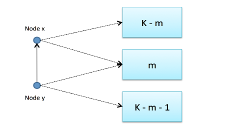
Figure 4: Depicting the condition $(x\in\Gamma_{y}~{},~{}y\notin\Gamma_{x}~{},~{}|\Gamma_{x}\cup\Gamma_{y}|=2K_{n}-m~{},~{}B_{xy}=1)$ for the calculation of $P_{21}(n,\theta_{n};m,\ell)$. Dashed lines emanating from a node $x$ stand for the set of nodes in $\Gamma_{x}$ and a dashed line between $x$ and $y$ is made bold if $B_{xy}=1$.

Now, using arguments similar to those that lead to (123), we get

$$P_{21}(n;\theta_{n};m,\ell)$$ (137)

$$= \sum\limits_{i,j=0}^{\ell-1}{K_{n}\choose i}{{K_{n}-1}\choose j}p_{n}^{i+j}(1-p_{n})^{2K_{n}-i-j-1}~{}\sum\limits_{i_{1},j_{1}=0}^{\ell-1-i,\ell-1-j}{K_{n}-m-1\choose i_{1}}{K_{n}-m\choose j_{1}}$$

$$~{}\cdot\left(\frac{p_{n}K_{n}}{n-1}\right)^{i_{1}+j_{1}}\left(1-\frac{p_{n}K_{n}}{n-1}\right)^{2K_{n}-2m-i_{1}-j_{1}-1}~{}\sum\limits_{u=0}^{\ell-1-\max{(i+i_{1},j+j_{1})}}{n-2K_{n}+m-1\choose u}$$

$$~{}\cdot({\mathbb{P}}\left[{(z\sim x)\cap(z\sim y)}\right])^{u}{n-2K_{n}+m-1-u\choose\ell-1-i-i_{1}-u}({\mathbb{P}}\left[{(z\sim x)\cap(z\sim y)^{c}}\right])^{\ell-1-u-i-i_{1}}$$

$$~{}\cdot{n-2K_{n}+m-\ell+i+i_{1}\choose\ell-1-j-j_{1}-u}\cdot({\mathbb{P}}\left[{(z\sim x)^{c}\cap(z\sim y)}\right])^{\ell-1-u-j-j_{1}}$$

$$~{}\cdot\left({\mathbb{P}}\left[{(z\sim x)^{c}\cap(z\sim y)^{c}}\right]\right)^{n-2K_{n}+m+1-2\ell+i+i_{1}+j+j_{1}+u}$$

with $z$ denoting an arbitrary node in $\mathcal{V}/(\{x,y\}\cup\Gamma_{x}\cup\Gamma_{y})$. In (137), the following notation is used in the conditioning arguments: $d_{x}(\Gamma_{x})=i$, $d_{y}(\Gamma_{y}/\{x\})=j$, $d_{x}(\Gamma_{y}/(\Gamma_{x}\cup\{x,y\}))=i_{1}$, $d_{y}(\Gamma_{x}/(\Gamma_{y}\cup\{x,y\}))=j_{1}$, and $u$ denotes the number of nodes in $\mathcal{V}/(\{x,y\}\cup\Gamma_{x}\cup\Gamma_{y})$ that are connected to both $x$ and $y$; i.e., $u=|\{z\in\mathcal{V}/(\{x,y\}\cup\Gamma_{x}\cup\Gamma_{y}):~{}(z\sim x)\cap(z\sim y)\}|$.

By direct comparison of (137) and (123), we find that

$$P_{21}(n;\theta_{n};m,\ell)\leq(1+o(1))(1-p_{n})^{-1}\left(1-\frac{p_{n}K_{n}}{n-1}\right)^{-1}P_{1}(n;\theta_{n};m,\ell-1)$$ (138)

as we note

$${K_{n}-1\choose j}\leq{K_{n}\choose j}\qquad\textrm{and}\qquad{K_{n}-m-1\choose i_{1}}\leq{K_{n}-m\choose i_{1}}$$

and use the asymptotic equivalencies

$${n-2K_{n}+m-1\choose u} = (1+o(1)){n-2K_{n}+m-2\choose u}$$

$${n-2K_{n}+m-1-u\choose\ell-1-i-i_{1}-u} = (1+o(1)){n-2K_{n}+m-2-u\choose(\ell-1)-i-i_{1}-u}$$

$${n-2K_{n}+m-\ell+i+i_{1}\choose\ell-1-j-j_{1}-u} = (1+o(1)){n-2K_{n}+m-2-(\ell-1)+i+i_{1}\choose(\ell-1)-j-j_{1}-u}$$

that are immediate from the following arguments: Pick any positive constants $c_{1}$ and $c_{2}$, and recall that $\lim_{n\to\infty}n-2K_{n}=\infty$ under the enforced assumptions. Then, for any $m=0,1,\ldots,K_{n}$, we have

$$\frac{{n-2K_{n}+m\pm c_{1}\choose c_{2}}}{{n-2K_{n}+m\choose c_{2}}} = \frac{(n-2K_{n}+m\pm c_{1})!}{(n-2K_{n}+m\pm c_{1}-c_{2})!}\cdot\frac{(n-2K_{n}+m-c_{2})!}{(n-2K_{n}+m)!}$$ (139)

$$= \frac{(n-2K_{n}+m\pm c_{1})\cdots(n-2K_{n}+m\pm c_{1}-c_{2}+1)}{(n-2K_{n}+m)\cdots(n-2K_{n}+m-c_{2}+1)}$$

$$= \prod_{i=0}^{c_{2}-1}\left(1\pm\frac{c_{1}}{n-2K_{n}+m-i}\right)$$

$$= (1\pm o(1))^{c_{2}}$$

$$= 1+o(1).$$

We now report (107) and Proposition 8.1 into (138), and get

$$P_{21}(n;\theta_{n};m,\ell)\leq(1+o(1))(1-p_{n})^{-1}{\mathbb{P}}\left[{D_{x,\ell-1}}\right]^{2},\qquad\ell=1,2,\ldots.$$ (140)

Using the tight bound obtained for ${\mathbb{P}}\left[{D_{x,\ell}}\right]$ in Proposition 7.1, this then yields

$$P_{21}(n;\theta_{n};m,\ell)\leq(1+o(1)){\mathbb{P}}\left[{D_{x,\ell}}\right]^{2}(1-p_{n})^{-1}\left(\frac{p_{n}K_{n}}{\ell}\left(1-\frac{K_{n}}{n-1}+\frac{1}{1-p_{n}}\right)\right)^{-2}$$ (141)

The claim (135) is now immediate as we note that $(1-p_{n})^{-1}=O(1)$ under the assumption that $\lim\sup_{n\to\infty}p_{n}<1$ and

$$\lim_{n\to\infty}\left(\frac{p_{n}K_{n}}{\ell}\left(1-\frac{K_{n}}{n-1}+\frac{1}{1-p_{n}}\right)\right)=\infty$$

since $p_{n}K_{n}=\Omega(\log n)$ from (79) and we have $\left(1-\frac{K_{n}}{n-1}+\frac{1}{1-p_{n}}\right)\geq 1$ from (133).

We now consider the second term $P_{22}(n,\theta_{n};m,\ell)$ in (134). In view of (135), it is clear that Proposition 8.2 will be established if we show that

$$P_{22}(n,\theta_{n};m,\ell)\leq(1+o(1))(1-p_{n})^{-1}{\mathbb{P}}\left[{D_{x,\ell}}\right]^{2},\qquad\ell=0,1,\ldots$$ (142)

for each $m=0,1,\ldots,K_{n}$ under the enforced assumptions. We proceed as before and note that under the condition $(x\in\Gamma_{y}~{},~{}y\notin\Gamma_{x}~{},~{}|\Gamma_{x}\cup\Gamma_{y}|=2K_{n}-m~{},~{}B_{xy}(p_{n})=0)$, nodes $x$ and $y$ do not have an edge in between, and both need to have $\ell$ neighbors among the $n-2$ nodes in $\mathcal{V}/\{x,y\}$. Otherwise, everything is just the same with the case of computing $P_{21}(n,\theta_{n};m,\ell)$ including the set sizes given in (136). Therefore, we have

$$P_{22}(n,\theta_{n};m,\ell)=P_{21}(n,\theta_{n};m,\ell+1),\qquad\ell=0,1,\ldots$$ (143)

for each $m=0,1,\ldots,K_{n}$. Now, we use (138) in (143) to get

$$P_{22}(n,\theta_{n};m,\ell) \leq (1+o(1))(1-p_{n})^{-1}\left(1-\frac{p_{n}K_{n}}{n-1}\right)^{-1}P_{1}(n;\theta_{n};m,\ell)$$

$$\leq (1+o(1))(1-p_{n})^{-1}{\mathbb{P}}\left[{D_{x,\ell}}\right]^{2},$$

where in the last step we used (107) and Proposition 8.1. This establishes (142), and the proof of Proposition 8.2 is now complete in view of (135) and (134).  

11 A proof of Proposition 8.3

We start as in the proof of Proposition 8.2 and condition on the event $(x\sim_{B}y)$ to get

$$P_{3}(n,\theta_{n};m,\ell)=p_{n}P_{31}(n,\theta_{n};m,\ell)+(1-p_{n})P_{32}(n,\theta_{n};m,\ell)$$ (144)

where

$$P_{31}(n,\theta_{n};m,\ell) = {\mathbb{P}}\left[{D_{x,\ell}\cap D_{y,\ell}~{}\big{|}~{}x\in\Gamma_{y}~{},~{}y\in\Gamma_{x}~{},~{}|\Gamma_{x}\cup\Gamma_{y}|=2K_{n}-m~{},~{}B_{xy}(p_{n})=1}\right]$$

$$P_{32}(n,\theta_{n};m,\ell) = {\mathbb{P}}\left[{D_{x,\ell}\cap D_{y,\ell}~{}\big{|}~{}x\in\Gamma_{y}~{},~{}y\in\Gamma_{x}~{},~{}|\Gamma_{x}\cup\Gamma_{y}|=2K_{n}-m~{},~{}B_{xy}(p_{n})=0}\right]$$

In what follows, we will compute $P_{31}(n,\theta_{n};m,\ell)$ and $P_{32}(n,\theta_{n};m,\ell)$ in turn. We will start by showing that

$$P_{31}(n,\theta_{n};m,\ell)=o\left({\mathbb{P}}\left[{D_{x,\ell}}\right]^{2}\right),\qquad\ell=1,2,\ldots$$ (145)

for each $m=0,1,\ldots,K_{n}$ under the enforced assumptions. To do so, we note that the condition $(x\in\Gamma_{y}~{},~{}y\in\Gamma_{x}~{},~{}|\Gamma_{x}\cup\Gamma_{y}|=2K_{n}-m~{},~{}B_{xy}(p_{n})=1)$ amounts to having

$$|\Gamma_{x}\cap\Gamma_{y}|=m,\quad|\Gamma_{x}/(\Gamma_{y}\cup\{x,y\})|=K_{n}-m-1,\quad\textrm{and}\quad|\Gamma_{y}/(\Gamma_{x}\cup\{x,y\})|=K_{n}-m-1$$ (146)

Also under this condition, nodes $x$ and $y$ do have an edge in between, and they just need to have $\ell-1$ additional neighbors among the $n-2$ nodes in $\mathcal{V}/\{x,y\}$. These facts are depicted in Figure 5.

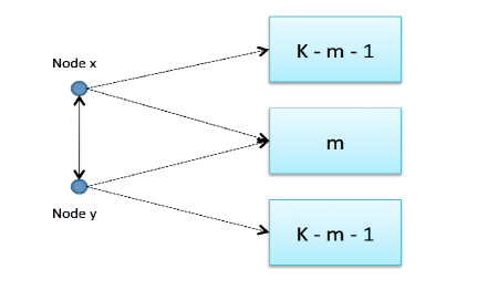
Figure 5: Depicting the condition $(x\in\Gamma_{y}~{},~{}y\in\Gamma_{x}~{},~{}|\Gamma_{x}\cup\Gamma_{y}|=2K_{n}-m~{},~{}B_{xy}=1)$ for calculating $P_{31}(n,\theta_{n};m,\ell)$. Dashed lines emanating from a node $x$ stand for the set of nodes in $\Gamma_{x}$ and a dashed line between $x$ and $y$ is made bold if $B_{xy}=1$.

Now, using arguments similar to those that lead to (123) and (137), we get

$$P_{31}(n;\theta_{n};m,\ell)$$ (147)

$$= \sum\limits_{i,j=0}^{\ell-1}{K_{n}-1\choose i}{{K_{n}-1}\choose j}p_{n}^{i+j}(1-p_{n})^{2K_{n}-i-j-2}~{}\sum\limits_{i_{1},j_{1}=0}^{\ell-1-i,\ell-1-j}{K_{n}-m-1\choose i_{1}}{K_{n}-m-1\choose j_{1}}$$

$$~{}\cdot\left(\frac{p_{n}K_{n}}{n-1}\right)^{i_{1}+j_{1}}\left(1-\frac{p_{n}K_{n}}{n-1}\right)^{2K_{n}-2m-i_{1}-j_{1}-2}~{}\sum\limits_{u=0}^{\ell-1-\max{(i+i_{1},j+j_{1})}}{n-2K_{n}+m\choose u}$$

$$~{}\cdot({\mathbb{P}}\left[{(z\sim x)\cap(z\sim y)}\right])^{u}{n-2K_{n}+m-u\choose\ell-1-i-i_{1}-u}({\mathbb{P}}\left[{(z\sim x)\cap(z\sim y)^{c}}\right])^{\ell-1-u-i-i_{1}}$$

$$~{}\cdot{n-2K_{n}+m-\ell+1+i+i_{1}\choose\ell-1-j-j_{1}-u}\cdot({\mathbb{P}}\left[{(z\sim x)^{c}\cap(z\sim y)}\right])^{\ell-1-u-j-j_{1}}$$

$$~{}\cdot\left({\mathbb{P}}\left[{(z\sim x)^{c}\cap(z\sim y)^{c}}\right]\right)^{n-2K_{n}+m+2-2\ell+i+i_{1}+j+j_{1}+u}$$

with $z$ denoting an arbitrary node in $\mathcal{V}/(\{x,y\}\cup\Gamma_{x}\cup\Gamma_{y})$. The notation used in the conditioning arguments of (147) are as follows: $d_{x}(\Gamma_{x})=i$, $d_{y}(\Gamma_{y}/\{x\})=j$, $d_{x}(\Gamma_{y}/(\Gamma_{x}\cup\{x,y\}))=i_{1}$, $d_{y}(\Gamma_{x}/(\Gamma_{y}\cup\{x,y\}))=j_{1}$, and $u$ denotes the number of nodes in $\mathcal{V}/(\{x,y\}\cup\Gamma_{x}\cup\Gamma_{y})$ that are connected to both $x$ and $y$; i.e., $u=|\{z\in\mathcal{V}/(\{x,y\}\cup\Gamma_{x}\cup\Gamma_{y}):~{}(z\sim x)\cap(z\sim y)\}|$.

By direct comparison of (147) and (137), we find that

$$P_{31}(n;\theta_{n};m,\ell)\leq(1+o(1))(1-p_{n})^{-1}\left(1-\frac{p_{n}K_{n}}{n-1}\right)^{-1}P_{21}(n;\theta_{n};m,\ell)$$ (148)

upon noting that

$${K_{n}-1\choose i}\leq{K_{n}\choose i}\qquad\textrm{and}\qquad{K_{n}-m-1\choose j_{1}}\leq{K_{n}-m\choose j_{1}}$$

and using the bounds

$${n-2K_{n}+m\choose u} = (1+o(1)){n-2K_{n}+m-1\choose u}$$

$${n-2K_{n}+m-u\choose\ell-1-i-i_{1}-u} = (1+o(1)){n-2K_{n}+m-1-u\choose\ell-1-i-i_{1}-u}$$

$${n-2K_{n}+m-\ell+1+i+i_{1}\choose\ell-1-j-j_{1}-u} = (1+o(1)){n-2K_{n}+m-\ell+i+i_{1}\choose\ell-1-j-j_{1}-u}$$

that are immediate from (139). The claimed result (145) follows immediately by reporting (135) into (148) and noting that

$$(1-p_{n})^{-1}\left(1-\frac{p_{n}K_{n}}{n-1}\right)^{-1}=O(1)$$ (149)

under the enforced assumptions; just recall that $\lim\sup_{n\to\infty}p_{n}<1$ and use (107).

In view of (145) and (144), Proposition 8.3 will be established if we show that

$$P_{32}(n,\theta_{n};m,\ell)\leq(1+o(1))(1-p_{n})^{-2}{\mathbb{P}}\left[{D_{x,\ell}}\right]^{2},\qquad\ell=0,1,\ldots$$ (150)

for each $m=0,1,\ldots,K_{n}$. In calculation of $P_{32}(n,\theta_{n};m,\ell)$, we need to consider the condition $(x\in\Gamma_{y}~{},~{}y\in\Gamma_{x}~{},~{}|\Gamma_{x}\cup\Gamma_{y}|=2K_{n}-m~{},~{}B_{xy}(p_{n})=0)$, where nodes $x$ and $y$ do not have an edge in between, and both need to have $\ell$ neighbors among the $n-2$ nodes in $\mathcal{V}/\{x,y\}$. This is the only difference between the probabilities $P_{31}(n,\theta_{n};m,\ell)$ and $P_{32}(n,\theta_{n};m,\ell)$. Except this difference, all statistical equivalencies and relations are the same including the set sizes given in (146). Therefore, it is immediate that

$$P_{32}(n,\theta_{n};m,\ell)=P_{31}(n,\theta_{n};m,\ell+1),\qquad\ell=0,1,\ldots$$ (151)

for each $m=0,1,\ldots,K_{n}$. We now use (148) in (151) to get

$$P_{32}(n,\theta_{n};m,\ell) \leq (1+o(1))(1-p_{n})^{-1}\left(1-\frac{p_{n}K_{n}}{n-1}\right)^{-1}P_{21}(n;\theta_{n};m,\ell+1)$$

$$\leq (1+o(1))(1-p_{n})^{-2}\cdot{\mathbb{P}}\left[{D_{x,\ell}}\right]^{2},$$

where in the last step we used the previously obtained bound (140) together with (107). This establishes (150), and the proof of Proposition 8.3 is now complete in view of (145) and (144).

References

• [1] I.ย F. Akyildiz, W.ย Su, Y.ย Sankarasubramaniam, and E.ย Cayirci. Wireless sensor networks: a survey. Computer networks, 38, 2002.
• [2] B.ย Bollobรกs. Random graphs. Cambridge university press, 2001.
• [3] H.ย Chan, A.ย Perrig, and D.ย Song. Random key predistribution schemes for sensor networks. In Proc. of IEEE S&P, 2003.
• [4] R.ย Diย Pietro, L.ย V. Mancini, A.ย Mei, A.ย Panconesi, and J.ย Radhakrishnan. Redoubtable sensor networks. ACM Trans. Inf. Syst. Secur., 11(3):13:1โ€“13:22, March 2008.
• [5] P.ย Erdล‘s and A.ย Rรฉnyi. On the strength of connectedness of random graphs. Acta Math. Acad. Sci. Hungar, pages 261โ€“267, 1961.
• [6] L.ย Eschenauer and V.ย Gligor. A key-management scheme for distributed sensor networks. In Proc. of ACM CCS, 2002.
• [7] T.ย I. Fenner and A.ย M. Frieze. On the connectivity of random m-orientable graphs and digraphs. Combinatorica, 2(4), 1982.
• [8] S.ย Janson, T.ย ลuczak, and A.ย Ruciล„ski. Random graphs. 2000. Wileyโ€“Intersci. Ser. Discrete Math. Optim, 2000.
• [9] K.ย Joag-Dev and F.ย Proschan. Negative association of random variables with applications. The Annals of Statistics, (1):286โ€“295, 1983.
• [10] B.ย Krishnan, A.ย Ganesh, and D.ย Manjunath. On connectivity thresholds in superposition of random key graphs on random geometric graphs. In Proc. of IEEE ISIT, pages 2389โ€“2393, 2013.
• [11] M.ย D. Penrose. Random Geometric Graphs. Oxford University Press, July 2003.
• [12] T.ย Philips, D.ย Towsley, and J.ย Wolf. On the diameter of a class of random graphs. IEEE Transactions on Information Theory, 36(2):285โ€“288, March 1990.
• [13] K.ย Rybarczyk. Sharp threshold functions for the random intersection graph via a coupling method. Electr. Journal of Combinatorics, 18:36โ€“47, 2011.
• [14] Y.ย Wang, G.ย Attebury, and B.ย Ramamurthy. A survey of security issues in wireless sensor networks. Communications Surveys Tutorials, IEEE, 8(2):2โ€“23, 2006.
• [15] Y. Xiao and V. K. Rayi and B. Sun and X. Du and F. Hu and M. Galloway. A survey of key management schemes in wireless sensor networks. Computer Communications, 30:2314 โ€“ 2341, 2007.
• [16] O.ย YaฤŸan. Random Graph Modeling of Key Distribution Schemes in Wireless Sensor Networks. PhD thesis, Department of Electrical and Computer Engineering, University of Maryland, College Park (MD), June 2011. Available online at http://hdl.handle.net/1903/11910.
• [17] O.ย YaฤŸan. Performance of the Eschenauer-Gligor key distribution scheme under an on/off channel. IEEE Transactions on Information Theory, 58(6):3821โ€“3835, June 2012.
• [18] O.ย YaฤŸan and A.ย M. Makowski. Designing securely connected wireless sensor networks in the presence of unreliable links. In Communications (ICC), 2011 IEEE International Conference on, pages 1โ€“5, 2011.
• [19] O.ย YaฤŸan and A.ย M. Makowski. On the gradual deployment of random pairwise key distribution schemes. In Proc. of WiOpt, 2011.
• [20] O.ย YaฤŸan and A.ย M. Makowski. Connectivity results for sensor networks under a random pairwise key predistribution scheme. In Information Theory Proceedings (ISIT), 2012 IEEE International Symposium on, pages 1797โ€“1801, 2012.
• [21] O.ย YaฤŸan and A.ย M. Makowski. Modeling the pairwise key predistribution scheme in the presence of unreliable links. IEEE Transactions on Information Theory, 59(3):1740โ€“1760, 2013.
• [22] O.ย YaฤŸan and A.ย M. Makowski. On the connectivity of sensor networks under random pairwise key predistribution. IEEE Transactions on Information Theory, 59(9):5754โ€“5762, 2013.
• [23] O.ย YaฤŸan and A.ย M. Makowski. On the scalability of the random pairwise key predistribution scheme: Gradual deployment and key ring sizes. Performance Evaluation, 70(7 8):493 โ€“ 512, 2013.
• [24] J.ย Zhao, O.ย YaฤŸan, and V.ย Gligor. k-connectivity in secure wireless sensor networks with physical link constraints - the on/off channel model. Arxiv, June 2012. Submitted to IEEE Transactions on Information Theory. Available online at arXiv:1206.1531 [cs.IT].
• [25] J.ย Zhao, O.ย YaฤŸan, and V.ย Gligor. Secure k-connectivity in wireless sensor networks under an on/off channel model. In Proc. of IEEE Intl. Symp. Info. Theory (ISIT), pages 2790โ€“2794, 2013.