Direct numerical simulation of pattern formation in subaqueous sediment

Abstract

We present results of direct numerical simulation of incompressible fluid flow over a thick bed of mobile, spherically-shaped particles. The algorithm is based upon the immersed boundary technique for fluid-solid coupling and uses a soft-sphere model for the solid-solid contact. Two parameter points in the laminar flow regime are chosen, leading to the emergence of sediment patterns classified as ‘small dunes’, while one case under turbulent flow conditions leads to ‘vortex dunes’ with significant flow separation on the lee side. Wavelength, amplitude and propagation speed of the patterns extracted from the spanwise-averaged fluid-bed interface are found to be consistent with available experimental data. The particle transport rates are well represented by available empirical models for flow over a plane sediment bed in both the laminar and the turbulent regimes.

1 Introduction

The process of erosion of particles from an initially flat subaqueous sediment layer and their deposition at certain preferential locations leads, under certain circumstances, to the amplification of small perturbations and gives rise to wave-like bed shapes which are commonly described as ripples or dunes. These sedimentary patterns are commonly observed in river and marine flows, as well as in various technical applications involving shear flow over a bed of mobile sediment particles. From an engineering point of view it is highly desirable to be able to predict the occurrence and the nature of this phenomenon, since the bed-form significantly influences flow characteristics such as resistance, mixing properties and sediment transport.

Most of the previous theoretical work on the formation of sediment patterns is based upon the notion that a flat bed is unstable with respect to perturbations of sinusoidal shape. It was Kennedy (1963) who first studied this instability problem by considering a potential flow solution, and over the years the concept has been applied by a number of researchers for a variety of flow conditions, in the laminar (Charru & Mouilleron-Arnould, 2002; Charru & Hinch, 2006) and turbulent regime (Richards, 1980; Sumer & Bakioglu, 1984; Colombini, 2004; Colombini & Stocchino, 2011). Invoking a disparity in time scales between the flow and the bed shape modification, most of the approaches have considered the bed shape as fixed for the purpose of the analysis. The hydrodynamic stability problem is then complemented by an expression for the particle flux as a function of the local bed shear stress at a given transversal section of the flow.

It is now generally accepted that the mechanism which destabilizes a flat sediment bed is the phase-lag between the perturbation in bed height and the bottom shear stress as a consequence of fluid inertia. A balance between this destabilizing mechanism and other stabilizing effects such as gravity (Engelund & Fredsoe, 1982) or phase-lag between bottom shear stress and the particle flow rate (Charru, 2006) is believed to result in instability of the bed at a certain preferred wavelength. Linear stability analysis is often applied to the problem in order to predict the most unstable wavelength; compared to experimental observations, however, predictions resulting from this approach can be broadly described as unsatisfactory, sometimes predicting pattern wavelengths which are off by an order of magnitude (Raudkivi, 1997; Langlois & Valance, 2007; Coleman & Nikora, 2009; Ouriemi et al., 2009).

Most available experimental studies report wavelengths of the developed bed-forms after they have undergone a coarsening process (the temporal evolution of the initial patterns to their ‘steady-state’ form), or possibly after they have coalesced with other bed-forms. There are several experimental studies which report on the initial wavelength and its development (Coleman & Melville, 1994; Betat et al., 2002; Coleman et al., 2003; Langlois & Valance, 2007; Ouriemi et al., 2009). However, the reported data is widely dispersed. Today it is still a challenge to capture the three-dimensional nature of the individual particle and fluid motion within the bed layer in a laboratory experiment, which in turn has hindered the assessment of the various theoretical approaches.

In the present work we numerically investigate the development of subaqueous patterns in a statistically uni-directional channel flow configuration both in the laminar and turbulent regimes. A sufficiently large number of freely-moving spherical particles are represented such that they form a realistic sediment bed in the simulation. To our knowledge, no attempt to numerically simulate the evolution of a bed of mobile sediment particles (leading to pattern formation) by means of direct numerical simulation (DNS), which resolves all the relevant length and time scales of the turbulent flow as well as the individual sediment particles, has been reported to the present date. The present study focuses on aspects related to the initial bed instabilities and their subsequent short-time development.

$(a)$

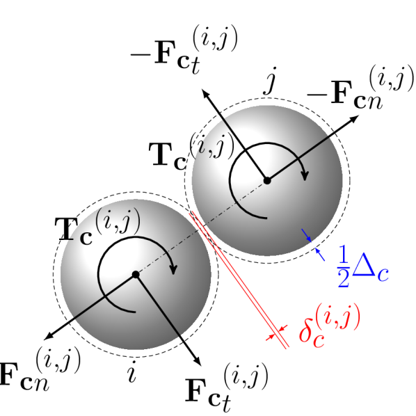
$(b)$

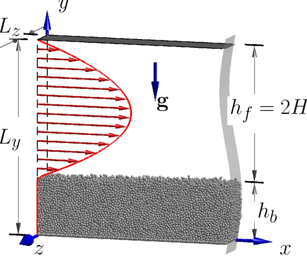
$(c)$

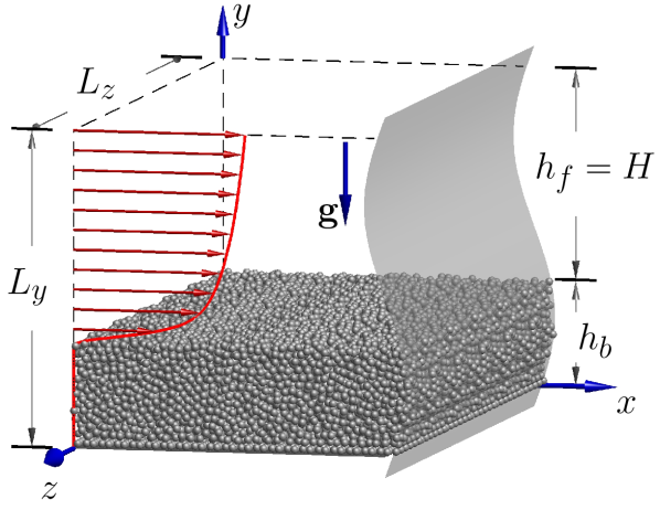
Figure 1: (a) Schematic showing the collision force $\mathbf{F_{c}}^{(i,j)}$ and torque $\mathbf{T_{c}}^{(i,j)}$ acting on particle with index $i$ during contact with particle $j$. The subscripts $n$ and $t$ indicate the normal and tangential components, respectively; $\Delta_{c}$ denotes the force range, and $\delta_{c}^{(i,j)}$ is the overlap length. (b) Computational domain and coordinate definition in cases LC1 and LC2. (c) The same for case TO1. The computational domains are periodic along the $x$- and $z$-directions with periods $L_{x}$, $L_{z}$, respectively.

2 Computational setup

2.1 Numerical method

The numerical treatment of the fluid-solid system is based upon the immersed boundary technique. The incompressible Navier-Stokes equations are solved with a second-order finite-difference method throughout the entire computational domain $\Omega$ (comprising the fluid domain $\Omega_{\mathrm{f}}$ and the domain occupied by the suspended particles $\Omega_{\mathrm{s}}$), adding a localized force term which serves to impose the no-slip condition at the fluid-solid interface. The particle motion is obtained via integration of the Newton equation for rigid body motion, driven by the hydrodynamic force (and torque) as well as gravity and the force (torque) resulting from inter-particle contact. Further information on the extensive validation of the direct numerical simulation (DNS) code on a whole range of benchmark problems can be found in Uhlmann (2005), Uhlmann & Dušek (2014) and further references therein. The code has been previously employed for the simulation of various particulate flow configurations (Uhlmann, 2008; Chan-Braun et al., 2011; García-Villalba et al., 2012; Kidanemariam et al., 2013).

In the present case, direct particle-particle contact contributes significantly to the dynamics of the system. In order to realistically simulate the collision process between the immersed particles, a discrete element model (DEM) based on the soft-sphere approach is coupled to the two-phase flow solver. The DEM used in the present work employs a linear mass-spring-damper system to model the collision forces, which are computed independently for each colliding particle pair. Any two particles are defined as ‘being in contact’ when the smallest distance between their surfaces, $\Delta$, becomes smaller than a force range $\Delta_{c}$ as illustrated in figure 1(a). The collision force is computed from the sum of an elastic normal component, a normal damping component and a tangential frictional component. The elastic part of the normal force component is a linear function of the penetration length $\delta_{c}\equiv\Delta_{c}-\Delta$, with a stiffness constant $k_{n}$. The normal damping force is a linear function of the normal component of the relative velocity between the particles at the contact point with a constant coefficient $c_{n}$. The tangential frictional force (the magnitude of which is limited by the Coulomb friction limit with a friction coefficient $\mu_{c}$) is a linear function of the tangential relative velocity at the contact point, again formulated with a constant coefficient denoted as $c_{t}$. A detailed description of the collision model and extensive validation tests with respect to available experimental data of a single particle colliding with a wall in a viscous fluid and in the case of bedload transport under laminar shear flow has been recently provided by Kidanemariam & Uhlmann (2014).

Case	$Re_{b}$	$Re_{\tau}$	$\rho_{p}/\rho_{f}$	$Ga$	$D^{+}$	$H/D$	$\Theta$	$[L_{x}\times L_{y}\times L_{z}]/D$	$\Delta x^{+}$	$D/\Delta x$	$N_{p}$
LC1	700	32.31	2.5	2.42	1.20	26.92	0.25	$307.2\times 76.8\times 12.8$	0.12	10	79073
LC2	700	32.08	2.5	1.97	1.20	26.71	0.37	$307.2\times 76.8\times 12.8$	0.12	10	79073
TO1	6022	290.34	2.5	28.37	11.59	25.05	0.17	$307.2\times 38.4\times 76.8$	1.16	10	263412

Table 1: Physical and numerical parameters of the simulations: $Re_{b}$ and $Re_{\tau}$ are the bulk and friction Reynolds numbers, respectively, $\rho_{p}/\rho_{f}$ is the particle-to-fluid density ratio, $Ga$ is the Galileo number, $D$ is the particle diameter, $H$ is the equivalent boundary layer thickness, $\Theta$ the Shields number, $L_{i}$ is the domain size in the $i$th coordinate direction, $\Delta x$ is the uniform mesh width and $N_{p}$ is the number of particles.

The four parameters which describe the collision process in the framework of this model ($k_{n}$, $c_{n}$, $c_{t}$, $\mu_{c}$) as well as the force range $\Delta_{c}$ need to be prescribed for each simulation. From an analytical solution of the linear mass-spring-damper system in an idealised configuration (considering a binary collision of uniformly translating spheres in vacuum and in the absence of external forces), a relation between the normal stiffness coefficient $k_{n}$ and the normal damping coefficient $c_{n}$ can be formed by introducing the dry restitution coefficient $\varepsilon_{d}$. This latter quantity is a material property, defined as the absolute value of the ratio between the normal components of the relative velocity post-collision and pre-collision. In the present simulations, $\Delta_{c}$ is set equal to one grid spacing $\Delta x$. The stiffness parameter $k_{n}$ has a value equivalent to approximately $17000$ times the submerged weight of the particles, divided by the particle diameter. The chosen value ensures that the maximum overlap $\delta_{c}$ over all contacting particle pairs is within a few percent of $\Delta_{c}$. The dry coefficient of restitution is set to $\varepsilon_{d}=0.3$ which together with $k_{n}$ fixes the value for $c_{n}$. Finally, the tangential damping coefficient $c_{t}$ was set equal to $c_{n}$, and a value of $\mu_{c}=0.4$ was imposed for the Coulomb friction coefficient. This set of parameter values for the contact model was successfully employed in the simulations of (featureless) bedload transport by Kidanemariam & Uhlmann (2014).

In order to account for the large disparity between the time scales of the particle collision process and those of the smallest flow scales, the Newton equation for particle motion is solved with a significantly smaller time step than the one used for solving the Navier-Stokes equations (by a factor of approximately one hundred), while keeping the hydrodynamic contribution to the force and torque acting upon the particles constant during the intermediate interval.

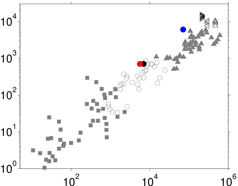
$Ga({2H}/{D})^{2}$

$Re_{b}$, $Re_{pipe}$

Figure 2: Different regimes of sediment bed patterns obtained in the pipe flow experiment of Ouriemi et al. (2009), shown in the parameter plane ($Re_{b}$,$Ga({2H}/{D})^{2}$): ‘flat bed in motion’ ($\blacksquare$); ‘small dunes’ ($\circ$); ‘vortex dunes’ ($\blacktriangle$). For the pipe flow data the Reynolds number $Re_{pipe}$ based upon the pipe diameter $d_{pipe}$ and the bulk velocity $q_{f}/d_{pipe}$ is used. The data points in the turbulent channel flow experiment of Langlois & Valance (2007) are indicated by: $D=100\mu m$ ($\vartriangle$); $D=250\mu m$ ($\vartriangleleft$); $D=500\mu m$ ($\vartriangleright$). The following symbols refer to the present simulations: $\bullet$, LC1; $\bullet$, LC2; $\bullet$, TO1.

2.2 Flow configuration and parameter values

The flow considered in this work is horizontal plane channel flow in a doubly-periodic domain as shown in figure 1$(b,c)$. Three simulations are performed, henceforth denoted as case LC1, case LC2 (both in the laminar flow regime) and case TO1 (in the turbulent regime). In cases LC1 and LC2 the domain is bounded in the vertical direction by two solid wall planes, whereas for reasons of computational cost in case TO1 an open channel is simulated, i.e. only the lower boundary plane corresponds to a no-slip wall, while a free-slip condition is imposed at the upper boundary plane. As shown in figure 1 the Cartesian coordinates $x$, $y$, and $z$ are aligned with the streamwise, wall-normal and spanwise directions, respectively, while gravity acts in the negative $y$-direction. The flow is driven by a horizontal pressure gradient at constant flow rate $q_{f}$ (per unit spanwise length) which results in a shear flow of height $h_{f}$ over a mobile bed of height $h_{b}$; spatial averages $\langle\overline{h}_{f}\rangle_{x}$ and $\langle\overline{h}_{b}\rangle_{x}$ of both quantities are defined in § 2.4; temporal averaging over the final period of the simulations is henceforth indicated by the operator $\langle\cdot\rangle_{t}$. The bulk Reynolds number of the flow is defined as $Re_{b}=2Hu_{b}/\nu$, where $u_{b}\equiv q_{f}/\langle\overline{h}_{f}\rangle_{xt}$ is the bulk velocity, $H$ is the equivalent boundary layer thickness (i.e. $H=\langle\overline{h}_{f}\rangle_{xt}/2$ in cases LC1, LC2 and $H=\langle\overline{h}_{f}\rangle_{xt}$ in case TO1, cf. figure 1$b,c$), and $\nu$ is the kinematic viscosity. Similarly, the friction Reynolds number is defined as $Re_{\tau}=u_{\tau}\langle\overline{h}_{f}\rangle_{xt}/\nu$, where the friction velocity $u_{\tau}$ is computed by extrapolation of the total shear stress to the fully-developed value of the wall-normal location of the average fluid-bed interface $\langle\overline{h}_{b}\rangle_{x}$. Further physical parameters are the ratio of particle to fluid density, $\rho_{p}/\rho_{f}$, the Galileo number $Ga=u_{g}D/\nu$ (where $u_{g}=((\rho_{p}/\rho_{f}-1)|\mathbf{g}|D)^{1/2}$ and $D$ the particle diameter), the Shields number $\Theta=u_{\tau}^{2}/u_{g}^{2}$ and the length scale ratio $H/D$; these together with the chosen numerical parameters are shown in table 1. The present simulations consumed a total of approximately 5 million core hours on the computing system SuperMUC at LRZ München. Typical runs of case TO1 were carried out on 576 cores.

Figure 2 shows the three parameter points of the present simulations in the plane spanned by $Re_{b}$ and $Ga({2H}/{D})^{2}$) in comparison to the laboratory experiments of Ouriemi et al. (2009) and Langlois & Valance (2007). Note that the former experiment was performed in pipe flow, whereas the latter was in plane channel flow. It can be seen that the cases LC1 and LC2 fall into the regime where the formation of ‘small dunes’ is expected while ‘vortex dunes’ can be anticipated in case TO1.

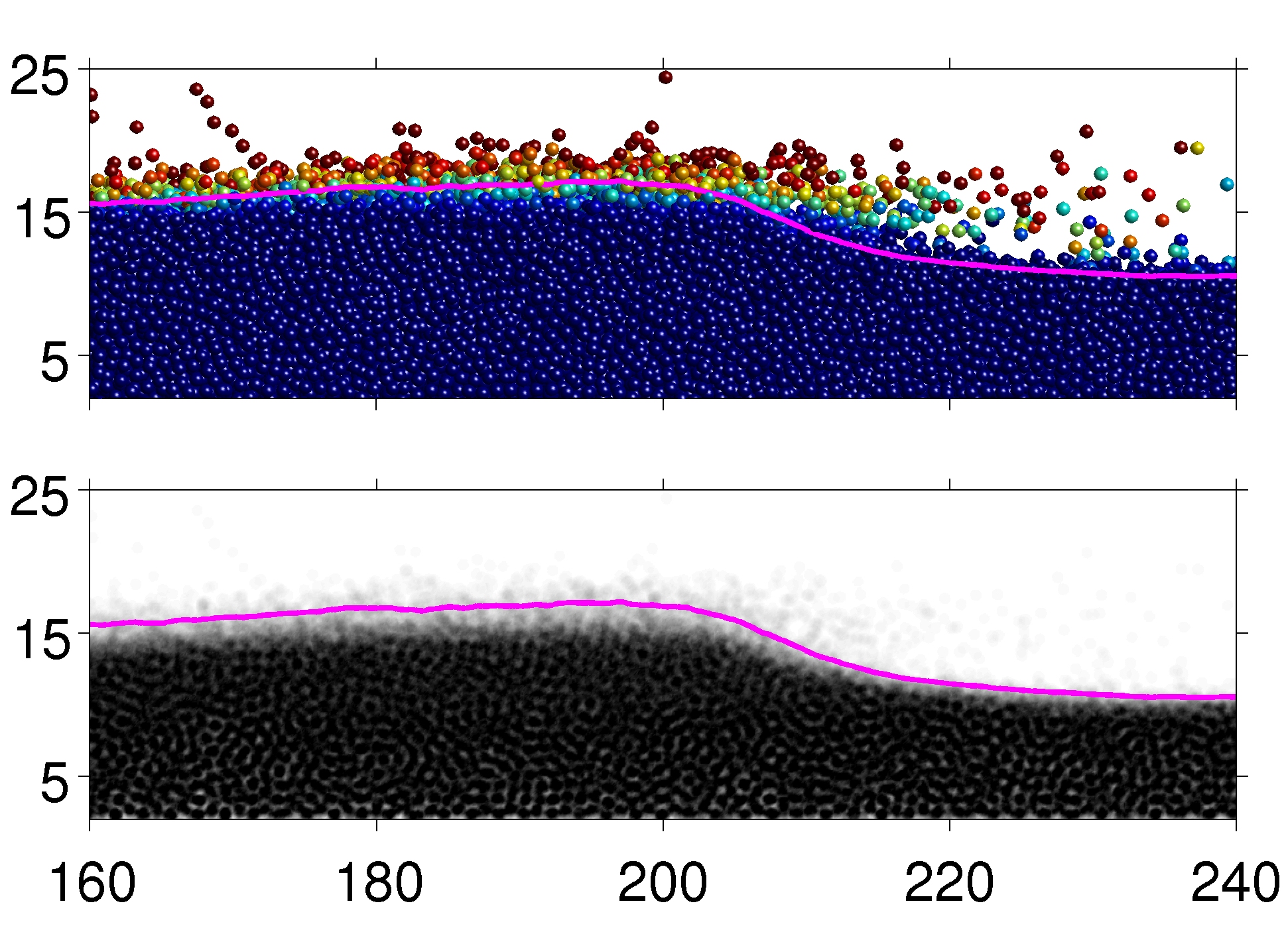
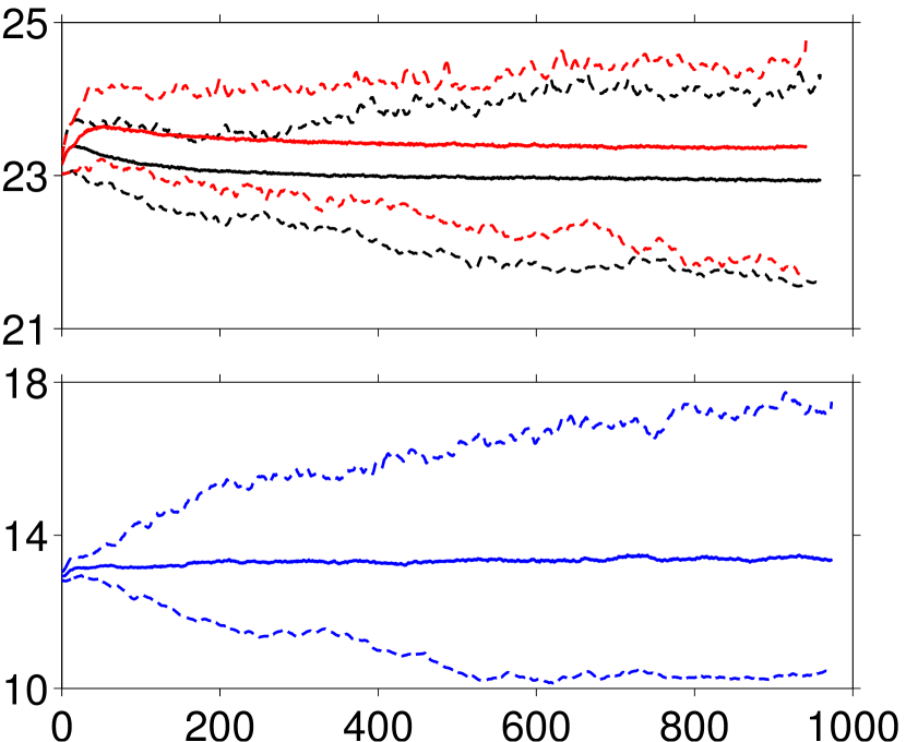
$(a)$ $\displaystyle\frac{y}{D}$ $(b)$ $\displaystyle\frac{y}{D}$ $x/D$    $(c)$ $\displaystyle\frac{y}{D}$ $(d)$ $\displaystyle\frac{y}{D}$ $t\,u_{b}/H$

Figure 3: (a) Close-up showing an instantaneous distribution of particles (colored according to their streamwise velocity) in case TO1. (b) The spanwise-averaged two-dimensional solid volume fraction $\langle\phi_{p}\rangle_{z}(x,y,t)$ corresponding to the snapshot shown in (a) displayed in greyscale. The extracted fluid-bed interface location $\overline{h}_{b}(x,t)$ is shown with a magenta colored line. (c) Time evolution of the bed height: $\langle\overline{h}_{b}\rangle_{x}(t)$ is shown as solid lines, $\min_{x}(\overline{h}_{b})$ and $\max_{x}(\overline{h}_{b})$ are shown as dashed lines. Black color is used for case LC1, red color for case LC2. (d) The same quantities as shown in (c), but for case TO1(see also the movies available as supplementary material).

2.3 Initiation of the simulations

The simulations were initiated as follows. In a first stage the initial sediment bed was generated by means of a simulation of particles settling (from random initial positions) under gravity and under solid-solid collisions but disregarding hydrodynamic forces. The result is a pseudo-randomly packed bed of initial bed thickness $h_{b}(t=0)$ above the bottom wall. Then the actual fully-coupled fluid-solid simulation is started with all particles being initially at rest. In cases LC1 and LC2, the initial fluid velocity field is set equal to a laminar Poiseuille flow profile with the desired flowrate in the interval $h_{b}(t=0)\leq y\leq L_{y}$ and zero elsewhere. After starting the simulation, individual particles are set into motion due to the action of hydrodynamic force/torque, and erosion takes place. In case TO1 the fluid-solid simulation was first run with all particles held fixed in order to develop a fully-turbulent field over the given sediment bed. After approximately $100$ bulk time units the particles were released, and the bed started to evolve away from its initial macroscopically flat shape, as discussed in the following.

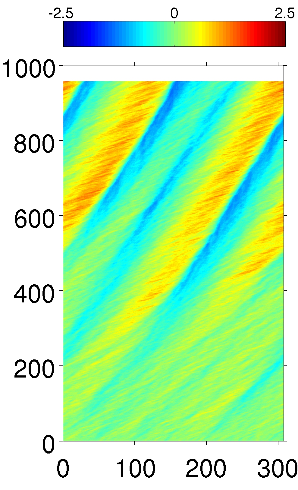
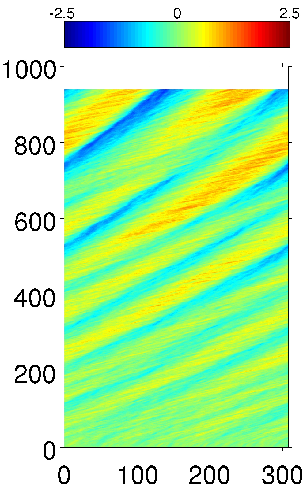
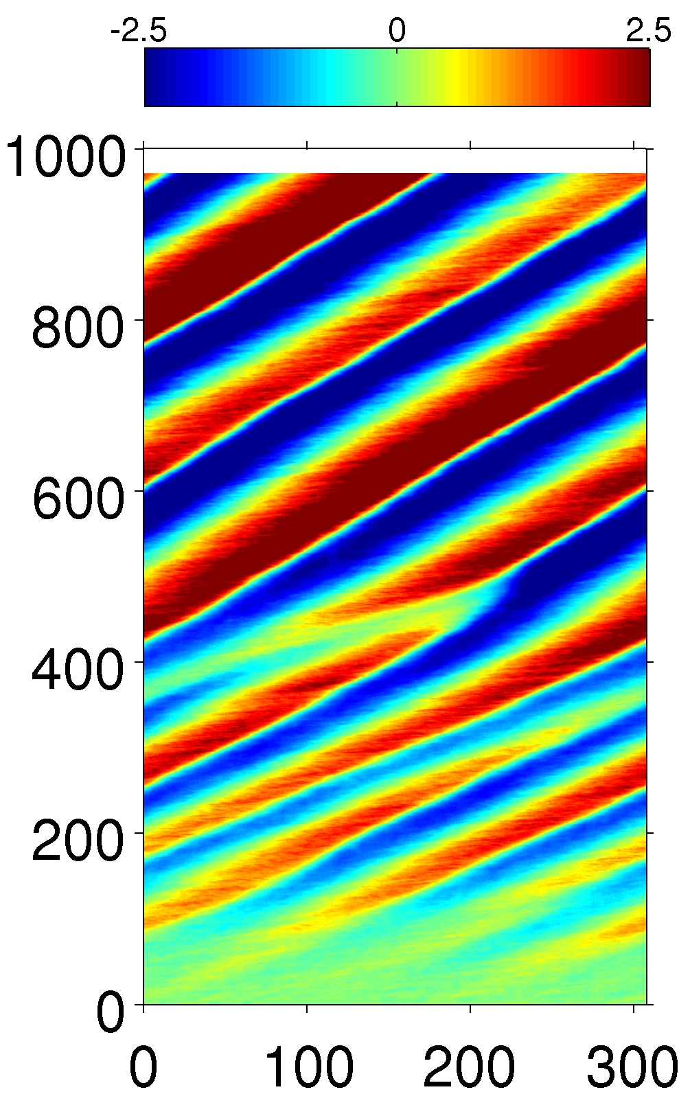
$(a)$ $t\,u_{b}/H$ $x/D$    $(b)$ $t\,u_{b}/H$ $x/D$    $(c)$ $t\,u_{b}/H$ $x/D$

Figure 4: Space-time evolution of the fluctuation of the fluid-bed interface location, $\overline{h}_{b}^{\prime}(x,t)=\overline{h}_{b}(x,t)-\langle\overline{h}_{b}\rangle_{x}(t)$, normalized with the particle diameter $D$: (a) case LC1; (b) case LC2; (c) case TO1.

2.4 Definition of the fluid-bed interface

The location of the interface between the fluid and the sediment bed has been determined in the following way. First, a solid phase indicator function $\phi_{p}(\mathbf{x},t)$ is defined which measures unity if $\mathbf{x}$ is located inside any particle and zero elsewhere. Spanwise averaging then yields $\langle\phi_{p}\rangle_{z}(x,y,t)$ which is a direct measure of the instantaneous, two-dimensional solid volume fraction. The spanwise-averaged fluid-bed interface location $\overline{h}_{b}(x,t)$ is finally extracted by means of a threshold value, chosen as $\langle\phi_{p}\rangle_{z}^{thresh}=0.1$ (Kidanemariam & Uhlmann, 2014), viz.

$$\overline{h}_{b}(x,t) = y\;\;|\;\langle\phi_{p}\rangle_{z}(x,y,t)=\langle\phi_{p}\rangle_{z}^{thresh}\;,$$ (1)

as illustrated in figure 3(b). The corresponding spanwise-averaged fluid height is then simply given by $\overline{h}_{f}(x,t)=L_{y}-\overline{h}_{b}(x,t)$. Figure 3(c,d) shows the time evolution of the streamwise average of the bed height defined in (1), $\langle\overline{h}_{b}\rangle_{x}(t)$, as well as its minimum and maximum values. It can be observed that after a small initial dilation $\langle\overline{h}_{b}\rangle_{x}$ quickly reaches an approximately constant value in all three cases. Contrarily, the maximum and minimum values of the bed elevation continue to diverge over the simulated interval of approximately $1000$ bulk time units, not reaching an equilibrium state.

3 Results

Space-time plots of the sediment bed height fluctuation with respect to the instantaneous streamwise average, defined as $\overline{h}_{b}^{\prime}(x,t)=\overline{h}_{b}(x,t)-\langle\overline{h}_{b}\rangle_{x}(t)$, are shown in figure 4. The emergence of dune-like patterns can be clearly observed, with a streamwise succession of alternating ridges and troughs forming shortly after start-up in all three cases. In the two simulations in the laminar regime we obtain similar fluctuation amplitudes. However, the propagation velocity is significantly larger in case LC2 (i.e. at larger Shields number) than in case LC1. The turbulent case TO1, on the other hand, is found to exhibit a higher growth rate, rapidly leading to enhanced fluctuation amplitudes as compared to both laminar cases.

$(a)$

$x/D$

$y/D$

$(b)$

$x/D$

Figure 5: Close-up of the instantaneous, spanwise-averaged solid-volume fraction $\langle\phi_{p}\rangle_{z}$ (plotted in greyscale) as well as the streamlines computed from a spanwise-averaged instantaneous flow field in the final phase of the simulated interval: $(a)$ case LC1; $(b)$ case TO1.

Furthermore, these space-time plots show the occasional occurrence of dune mergers with a subsequent increase of wavelength and an apparent decrease of the propagation speed. For times $t\gtrsim 550H/u_{b}$ the sediment bed patterns in the turbulent case TO1 (cf. figure 4$c$) remain roughly invariant with two distinct dunes featuring somewhat different elevation amplitudes.

A visualization of the fluid-bed interface and the streamlines of the spanwise averaged flow field towards the end of the simulated intervals is shown in figure 5. It is found that the patterns in the laminar cases indeed correspond to ‘small dunes’ in the terminology of Ouriemi et al. (2009), and to ‘vortex dunes’ with significant separation on the lee-side in the turbulent case (the graph for case LC2 is similar to case LC1 and has been omitted). These results are, therefore, consistent with the regime classification based upon the channel (or pipe) Reynolds number proposed by these authors (cf. figure 2).

The instantaneous two-point correlation of the bed height fluctuation as a function of streamwise separations $r_{x}$, defined as $R_{h}(r_{x},t)=\langle\overline{h}_{b}^{\prime}(x,t)\,\overline{h}_{b}^{\prime}(x+r_{x},t)\rangle_{x}$, exhibits a clear negative minimum in all of the present cases (figure omitted). Therefore, we can define an average pattern wavelength $\lambda_{av}$ as twice the streamwise separation at which the global minimum of $R_{h}$ occurs. The time evolution of the mean wavelength $\lambda_{av}$, normalized by the particle diameter, is shown in figure 6$(a)$. Also indicated with horizontal dashed lines in the graph are the wavelengths of the second to sixth harmonics in the present computational domain (recall that $L_{x}/D=307.2$ throughout the present work). It can be seen that for short times the wavelength $\lambda_{av}$ in the turbulent case TO1 exhibits several fast oscillations between $L_{x}/5$ and $L_{x}/2$ before approximately settling at a value near $L_{x}/3$ (i.e. $\lambda_{av}/D\approx 102$) for some 200 bulk time units. Starting with time $tu_{b}/H\approx 250$ the average wavelength then grows at an increasing rate, settling again at $\lambda_{av}\approx L_{x}/2=153.6D$ until the end of the simulated interval.

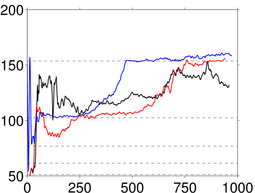
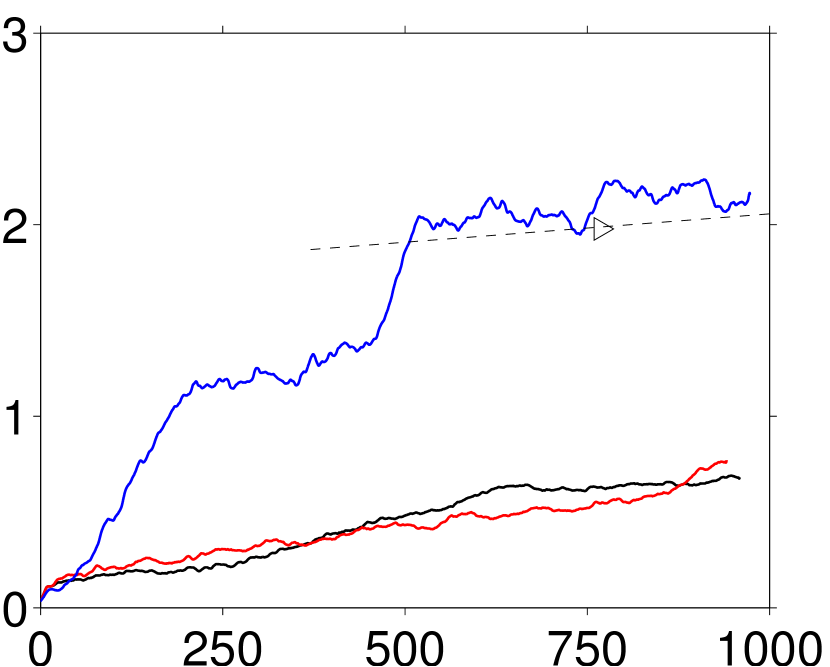
$(a)$ $\lambda_{av}/D$ $t\,u_{b}/H$ $(b)$ $\langle\overline{h}_{b}^{\prime}\overline{h}_{b}^{\prime}\rangle_{x}^{1/2}/D$ $t\,u_{b}/H$

Figure 6: (a) Time evolution of the mean wavelength of the sediment bed height normalized with the particle diameter. The dashed lines indicate the wavelengths of the second to sixth streamwise harmonics in the current domain. (b) Time evolution of the r.m.s. sediment bed height. The dashed line shows the fit obtained by Langlois & Valance (2007, figure 6$a$) for their case with $Re_{2H}=15130$, $\Theta=0.099$, $H/D=35$. Note that this fit was obtained for $t\geq 740u_{b}/H$ (their first data point is indicated by the symbol ‘$\vartriangleright$’). In both graphs solid lines with the following colors correspond to the present cases:   LC1,   LC2,   TO1.

Contrarily, the two laminar cases have a less oscillatory initial evolution. Case LC2 first settles into a plateau-like state (with $\lambda_{av}\approx L_{x}/3$) after approximately 250 elapsed bulk time units. Subsequently the wavelength corresponding to the second harmonic ($\lambda_{av}\approx L_{x}/2$) grows in amplitude and becomes dominant after approximately 750 bulk units. Case LC1 does not appear to settle into any of the harmonic wavelengths of the current domain, exhibiting an average wavelength in the range of $100-150$ particle diameters for the most part of the simulated interval. In turbulent channel flow experiments, Langlois & Valance (2007) have determined values of the initial pattern wavelength of $\lambda/D\approx 100-150$, roughly independent of the grain size. Upon scaling with the equivalent boundary layer thickness, the average pattern wavelengths in the three cases of the present work measure $3-6.5H$, except for a few initial bulk time units. This range is comparable to the range found for the initial wavelength of the ‘small dunes’ in pipe flow reported as $2.5-12.6H$ by Ouriemi et al. (2009, figure 7$b$) and for the ‘vortex dune’ data shown in their figure 3$(c)$, where an initial wavelength of $4H$ is observed.

Let us turn to the amplitude of the sediment patterns. The evolution of the r.m.s. value of the fluid-bed interface location is plotted in figure 6(b). The fact that no saturation is observed by the end of the simulated intervals is consistent with experimental observations, where it was found that even after an order of magnitude longer times the amplitude of the patterns continues to grow (the intervals simulated in the current work correspond to roughly one minute in the experiments of Langlois & Valance, 2007, conducted over more than one hour). Both of the present laminar cases exhibit growth at an approximately constant rate (with a slope of $6\cdot 10^{-4}$ in the units of figure 6b). Contrarily, the time evolution in the turbulent case TO1 is quasi-linear with different slopes in different time intervals. The initial growth of the turbulent case (for times up to $tu_{b}/H\approx 200$) and the growth in the interval $450\lesssim tu_{b}/H\lesssim 500$ are approximately ten times higher than the growth in the laminar cases, while in the remaining two intervals the growth rate is comparable to the laminar value. As can be seen in figure 6(b), the time evolution in the final period of case TO1 is roughly equivalent to the one determined by Langlois & Valance (2007) in turbulent flow at comparable parameter values ($Re_{2H}=15130$, $\Theta=0.099$, $H/D=35$).

The propagation speed of the patterns can be determined from the shift of the maximum of the two-point/two-time correlation of the fluid-bed interface fluctuation $\overline{h}_{b}^{\prime}(x,t)$. It turns out that the patterns in case LC1 propagate at a relatively constant speed of approximately $0.011u_{b}$, while the propagation velocity decreases with time during the coarsening process in cases LC2 and TO1, reaching values of $0.026u_{b}$ and $0.035u_{b}$, respectively, in the final period of the current simulations. The latter number is consistent with the range of values reported for ‘vortex dunes’ by Ouriemi et al. (2009, figure 3$b$).

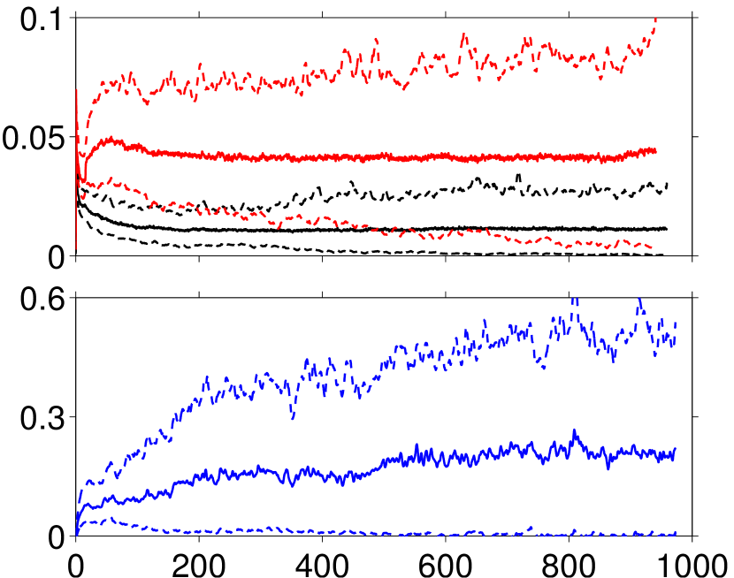
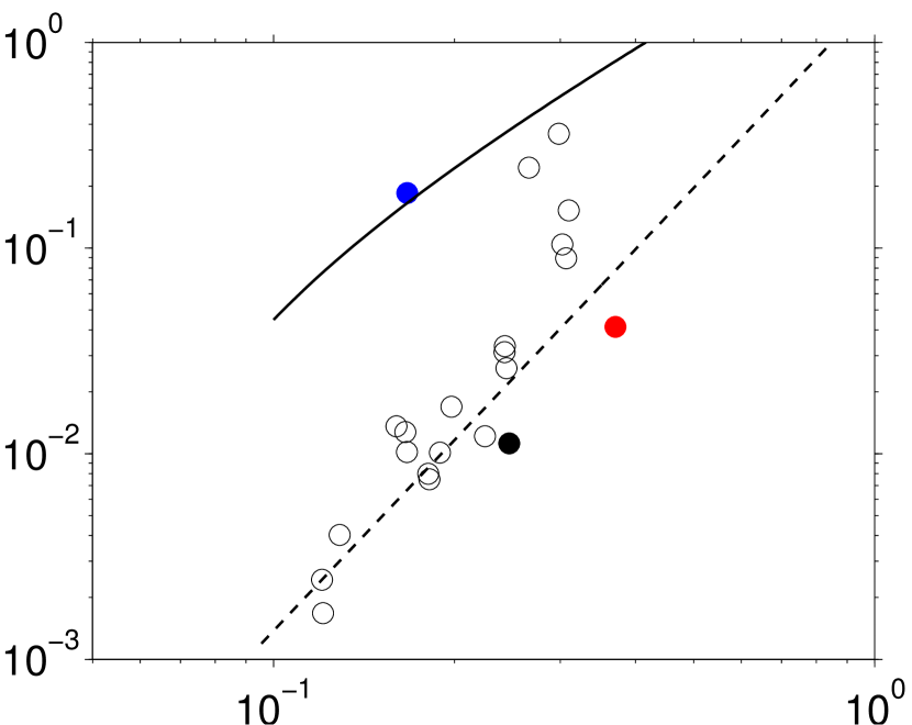
$(a)$ $\langle\overline{q}_{p}\rangle_{x}/q_{v}$ $(b)$ $\langle\overline{q}_{p}\rangle_{x}/q_{i}$ $t\,u_{b}/H$ $(c)$ $\langle\overline{q}_{p}\rangle_{xt}/q_{i}$ $\langle\overline{q}_{p}\rangle_{xt}/q_{v}$, $\Theta$

Figure 7: Analysis of the volumetric particle flow rate (per unit spanwise length), $\overline{q}_{p}(x,t)$. (a) The time evolution of the streamwise average value, $\langle\overline{q}_{p}\rangle_{x}(t)$ in cases LC1 (black color) and LC2 (red color) is shown with solid lines. The viscous scale $q_{v}=Ga^{2}\,\nu$ is used for the purpose of normalization. Additionally, the two dashed lines in each case indicate the respective minimum and maximum values ($\min_{x}\overline{q}_{p}$, $\max_{x}\overline{q}_{p}$). (b) The same quantity in case TO1, using the inertial scale $q_{i}=u_{g}D$ for normalization. (c) The value of the time average $\langle\overline{q}_{p}\rangle_{xt}$ over the final part of the simulations plotted versus the Shields number $\Theta$: $\bullet$, LC1; $\bullet$, LC2; $\bullet$, TO1. Note the different scalings ($q_{v}$ in the laminar cases, $q_{i}$ in the turbulent case). The open circles are for featureless bedload transport in laminar flow (Kidanemariam & Uhlmann, 2014); the dashed line is the fit $\langle\overline{q}_{p}\rangle_{xt}/q_{v}=1.66\,\Theta^{3.08}$ from that reference. The solid line is the Wong & Parker (2006) version $\langle\overline{q}_{p}\rangle_{xt}/q_{i}=4.93\,(\Theta-0.047)^{1.6}$ of the Meyer-Peter & Müller (1948) formula for turbulent flow.

The volumetric particle flow rate (per unit spanwise length), $\overline{q}_{p}(x,t)$, is analyzed in figure 7. The solid lines in figure 7$(a,b)$ show the temporal evolution of the streamwise average $\langle\overline{q}_{p}\rangle_{x}(t)$, which is observed to reach approximately constant values after a few hundred bulk time units in all cases. The continuous growth of the pattern amplitudes (cf. figure 6$b$) seems to have only a mild influence upon the total particle flow rate, irrespective of the flow regime. These graphs also show for each instant the maximum and minimum values (in space) of the particle flow rate, drawn as dashed lines. Although these extrema curves are noisier, it can be observed that the maxima continue to grow until the end of the simulations, consistent with the increase in the amplitude of the propagating patterns. Of particular interest in view of applications is the scaling of the particle transport rates, typically expressed as a function of the Shields number $\Theta$. Figure 7$(c)$ shows the space-averaged values, additionally averaged in time over the final part of the simulations, denoted as $\langle\overline{q}_{p}\rangle_{xt}$. It is found that the present values of $\langle\overline{q}_{p}\rangle_{xt}/q_{v}$ (where $q_{v}=Ga^{2}\,\nu$) in the two laminar cases are only slightly below the (approximately) cubic power law fitted by Kidanemariam & Uhlmann (2014) to their simulation data for featureless bedload transport. It is obviously not possible to infer scaling from two data points. However, if a power law of the particle flow rate as a function of the Shields number is assumed, the present laminar data suggest a cubic variation. Turning to the turbulent case TO1, figure 7$(c)$ shows that the value for $\langle\overline{q}_{p}\rangle_{xt}/q_{i}$ (with the inertial scaling $q_{i}=u_{g}\,D$) is very close to the value given by the empirical law of Wong & Parker (2006), which in turn is a modified version of the Meyer-Peter & Müller (1948) formula for turbulent flow. Wong & Parker’s formula is valid for plane sediment beds. The fact that the present data agrees well with that prediction together with the observed mild variation in time (cf. figure 7$b$) shows that the presence of ‘vortex dunes’ does not strongly affect the net particle transport rate.

4 Summary and conclusion

We have performed direct numerical simulation of the flow over an erodible bed of spherical sediment particles above both the threshold for particle mobility and for pattern formation. Two cases in laminar flow (with different Galileo and Shields numbers) lead to the formation of ‘small dunes’, while one case under turbulent flow conditions exhibits ‘vortex dunes’, consistently with the regime classification of Ouriemi et al. (2009). The reconstruction of the fluid-bed interface from a spanwise-averaged solid volume fraction (involving a threshold value) has allowed us to analyze the length scales, amplitude and propagation velocity of the sediment patterns in detail. In all three respects, the results of the present simulations are found to be consistent with available experimental data.

We have observed that the continuing growth of the dune patterns, which have not reached a statistically stationary state after approximately 1000 bulk time units, does not strongly affect the net volumetric particle transport rates. In the two laminar cases the particle flow rate (per unit span) is consistent with a cubic power law as a function of the Shields number; these values are found to be not far from those obtained in featureless bedload transport. The value pertaining to the turbulent case is very well predicted by the transport law of Wong & Parker (2006) which is derived for turbulent flow in the presence of a plane mobile bed. The present results therefore seem to suggest that the presence of ‘small dunes’ as well as that of ‘vortex dunes’ up to the amplitudes encountered in the present simulations does not lead to a modification of the net particle transport rate which would require a correction of the respective transport laws. This conclusion should be reassessed in the future when much longer temporal intervals can be covered.

The present work demonstrates that the DNS-DEM approach to sediment pattern formation is feasible today. Although still costly in terms of computational resources, it is already possible to address some of the outstanding questions with this method. Some aspects which are of importance in geophysical applications (such as reaching the fully rough turbulent regime, guaranteeing an asymptotically large computational domain and integrating over asymptotically long temporal intervals) still present a considerable computational challenge.

As a next step, the streamwise length of the computational domain should be extended in order to reduce the influence of the discreteness of the numerical harmonics upon the pattern wavelength. Conversely, shrinking the box length will allow to reveal the smallest amplified wavelength of the sedimentary patterns. Finally, an in-depth investigation of the flow field which develops over the time-dependent sediment bed can be carried out based upon the simulation data. Preliminary visualization suggests that in the turbulent case the coherent structures leave their footprint in the bed shape, visible as longitudinal ridges and troughs superposed on the roughly two-dimensional dune patterns. Such an analysis is left for future work.

This work was supported by the German Research Foundation (DFG) through grant UH 242/2-1. The computer resources, technical expertise and assistance provided by the staff at LRZ München (grant pr58do) are thankfully acknowledged.

Movies of the particle motion are available as ancillary files along with the arXiv submission and from the following URL:

http://www.ifh.kit.edu/dns_data

References

- Betat et al. (2002) Betat, A., Kruelle, C. A., Frette, V. & Rehberg, I. 2002 Long-time behavior of sand ripples induced by water shear flow. Eur. Phys. J. E. Soft Matter 8 (5), 465–76.
- Chan-Braun et al. (2011) Chan-Braun, C., García-Villalba, M. & Uhlmann, M. 2011 Force and torque acting on particles in a transitionally rough open-channel flow. J. Fluid Mech. 684, 441–474.
- Charru (2006) Charru, F. 2006 Selection of the ripple length on a granular bed sheared by a liquid flow. Phys. Fluids 18 (12), 121508.
- Charru & Hinch (2006) Charru, F. & Hinch, E. J. 2006 Ripple formation on a particle bed sheared by a viscous liquid. Part 1. Steady flow. J. Fluid Mech. 550, 111–121.
- Charru & Mouilleron-Arnould (2002) Charru, F. & Mouilleron-Arnould, H. 2002 Instability of a bed of particles sheared by a viscous flow. J. Fluid Mech. 452, 303–323.
- Coleman et al. (2003) Coleman, S. E., Fedele, J. J. & Garcia, M. H. 2003 Closed-Conduit Bed-Form Initiation and Development. J. Hydraul. Eng. 129 (December), 956–965.
- Coleman & Melville (1994) Coleman, S. E. & Melville, B. W. 1994 Bed-form development. J. Hydraul. Eng. 120 (4), 544–560.
- Coleman & Nikora (2009) Coleman, S. E. & Nikora, V. I. 2009 Bed and flow dynamics leading to sediment-wave initiation. Water Resour. Res. 45 (4), n/a–n/a.
- Colombini (2004) Colombini, M. 2004 Revisiting the linear theory of sand dune formation. J. Fluid Mech. 502, 1–16.
- Colombini & Stocchino (2011) Colombini, M. & Stocchino, a. 2011 Ripple and dune formation in rivers. J. Fluid Mech. 673, 121–131.
- Engelund & Fredsoe (1982) Engelund, F. & Fredsoe, J. 1982 Sediment Ripples and Dunes. Annu. Rev. Fluid Mech. 14 (1), 13–37.
- García-Villalba et al. (2012) García-Villalba, M., Kidanemariam, A. G & Uhlmann, M. 2012 DNS of vertical plane channel flow with finite-size particles: Voronoi analysis, acceleration statistics and particle-conditioned averaging. Int. J. Multiph. Flow 46, 54–74.
- Kennedy (1963) Kennedy, J. F. 1963 The mechanics of dunes and antidunes in erodible-bed channels. J. Fluid Mech. 16 (4), 521–544.
- Kidanemariam & Uhlmann (2014) Kidanemariam, A.G. & Uhlmann, M. 2014 Interface-resolved direct numerical simulation of the erosion of a sediment bed sheared by laminar flow. Int. J. Multiphase Flow (submitted).
- Kidanemariam et al. (2013) Kidanemariam, A. G., Chan-Braun, C., Doychev, T. & Uhlmann, M. 2013 Direct numerical simulation of horizontal open channel flow with finite-size, heavy particles at low solid volume fraction. New J. Phys. 15 (2), 025031.
- Langlois & Valance (2007) Langlois, V. & Valance, A. 2007 Initiation and evolution of current ripples on a flat sand bed under turbulent water flow. Eur. Phys. J. E. Soft Matter 22 (3), 201–8.
- Meyer-Peter & Müller (1948) Meyer-Peter, E. & Müller, R. 1948 Formulas for bed-load transport. In Proc. 2nd Meeting, pp. 39–64. IAHR, Stockholm, Sweden.
- Ouriemi et al. (2009) Ouriemi, M., Aussillous, P. & Guazzelli, É. 2009 Sediment dynamics. Part 2. Dune formation in pipe flow. J. Fluid Mech. 636, 295–319.
- Raudkivi (1997) Raudkivi, A. J. 1997 Ripples on Stream Bed. J. Hydraul. Eng. 123 (1), 58–64.
- Richards (1980) Richards, K. J. 1980 The formation of ripples and dunes on an erodible bed. J. Fluid Mech. 99 (3), 597–618.
- Sumer & Bakioglu (1984) Sumer, B. M. & Bakioglu, M. 1984 On the formation of ripples on an erodible bed. J. Fluid Mech. 144, 177–190.
- Uhlmann (2005) Uhlmann, M. 2005 An immersed boundary method with direct forcing for the simulation of particulate flows. J. Comput. Phys. 209 (2), 448–476.
- Uhlmann (2008) Uhlmann, M. 2008 Interface-resolved direct numerical simulation of vertical particulate channel flow in the turbulent regime. Phys. Fluids 20 (5), 053305.
- Uhlmann & Dušek (2014) Uhlmann, M. & Dušek, J. 2014 The motion of a single heavy sphere in ambient fluid: a benchmark for interface-resolved particulate flow simulations with significant relative velocities. Int. J. Multiphase Flow 59, 221–243.
- Wong & Parker (2006) Wong, M. & Parker, G. 2006 Reanalysis and correction of bed-load relation of Meyer-Peter and Müller using their own database. J. Hydr. Eng. 132 (11), 1159–1168.