We propose here a new model termed as the Differential Equation Model for the first $0_{1}^{+}\rightarrow 2_{1}^{+}$ state excitation energy E2 of a given even-even nucleus, according to which the energy E2 is expressed in terms of its derivatives with respect to the neutron and proton numbers. This is based on a similar derivative equation satisfied by its complementary physical quantity namely the Reduced Electric Quadrupole Transition Probability B(E2)$\uparrow$ in a recently developed model. Although the proposed differential equation for E2 has been perceived on the basis of its close similarity to B(E2)$\uparrow$, its theoretical foundation otherwise has been clearly demonstrated. We further exploit the very definitions of the derivatives occurring in the differential equation in the model to obtain two different recursion relations for E2, connecting in each case three neighboring even-even nuclei from lower to higher mass numbers and vice-verse. We demonstrate their numerical validity using the available data throughout the nuclear chart and also explore their possible utility in predicting the unknown E2 values.

DIFFERENTIAL EQUATION MODEL FOR THE FIRST $0_{1}^{+}\rightarrow 2_{1}^{+}$ STATE EXCITATION ENERGY E2 OF EVEN-EVEN NUCLEI$*$

$*$ This is a slightly modified version of the article submitted for publication in Int. Jou. of Mod. Phys. (2014).

I Introduction

Reduced electric quadrupole transition probability B(E2)$\uparrow$ and its complimentary quantity, namely the first $0_{1}^{+}\rightarrow 2_{1}^{+}$ state excitation energy E2 for a even-even nucleus play crucial roles for the study of excited states of nuclei and more importantly the inherent nuclear structure. Such studies got a boost with the advent of isotope facilities providing a large amount of experimental data for several nuclides throughout the nuclear chart. The existence of a large volume of experimental data led Raman et al. rmn at the Oak Ridge Nuclear Data Project rmn ; rm3 to make a comprehensive analysis of all those data, in preparing the most sought-after experimentally adopted data table for both the above two physical quantities. Of late, Pritychenko et al. prt followed the process in compiling the newly emerging data sets for even-even nuclei near $N\sim Z\sim$ 28. These new data including the old set obviously put a challenge for the nuclear theorists to understand them.

Theoretically, possible existence of symmetry in nuclear dynamics first explored in developing mass formulas such as the Garvey-Kelson gkl mass formula that connects masses of six neighboring nuclei, got into the domain of properties of the excited states. In this regard possible existence of such symmetry led Ross and Bhadurirbh in developing difference equations involving both B(E2)$\uparrow$ and the E2 excitation energies of the neighboring even-even nuclei. Patnaik et al. pat on the other hand have also succeeded in establishing even more simpler difference equations connecting these values of four neighboring even-even nuclei.

Just recently wedem have succeeded in developing a new model for the B(E2)$\uparrow$, termed as the Differential Equation Model (DEM) according to which, the B(E2)$\uparrow$ value of a given even-even nucleus is expressed in terms of its derivatives with respect to the neutron and proton numbers. Since these two quantities more or less complement each other, it is expected that the excitation energy E2 should also satisfy a similar differential equation. Therefore in the present work with this view in the background, we propose a similar model for E2 and explore its validity and utility in predicting hitherto unknown data. It is needless to stress here that any relation in the form of a differential equation of any physical quantity is intrinsically sound enough to posses a good predictive ability. This philosophy has been well demonstrated in case of B(E2)$\uparrow$ predictions dem just recently, and also over the recent years in the development inm ; in2 ; in3 ; in5 of the Infinite Nuclear Matter (INM) model of atomic nuclei specifically for the prediction in5 of nuclear masses. We should also note here that the development of the Differential Equation Model for the B(E2)$\uparrow$ and presently for E2 is also based on the local energy relation of the INM model, which happens to be an important component of the ground-state energy of a nucleus signifying its individual characteristic nature.

In Sec. II, we show how such a relation in the form of a differential equation for E2 can be formulated followed by its possible theoretical justification. Sec. III deals with how the same differential equation can be used to derive two recursion relations in E2, connecting in each case three different neighboring even-even nuclei. Finally we present in Section IV, their numerical validity when subjected to the known rmn experimental data throughout the nuclear chart, and their possible utility in predicting its unknown values.

II Derivation of the Differential Equation for the First $0_{1}^{+}\rightarrow 2_{1}^{+}$ State Excitation Energy E2

As mentioned above that the development of the DEM model both for the B(E2)$\uparrow$ and presently for E2 owes its origin to the local energy differential equation in the INM model of atomic nuclei. Physically the local energy $\eta$ embodies all the characteristic properties of a given nucleus, mainly the shell and deformation, and has been explicitly shown rcn to carry the shell-structure. Therefore it is likely to have some characteristic correspondence with the properties of excited states of a given nucleus in general and in particular, the reduced transition probability $B(E2)\uparrow$ and its complementary quantity E2. Accordingly the $\eta$-equation as well as the B(E2)$\uparrow$-equation [see for instance the Eqs. (1 and 4) of the DEM model dem ] can be used as an ansatz to satisfy a similar relation involving the E2 value of a given even-even nucleus. As a result we write on analogy, a similar equation for E2 as

$${E2[N,Z]/A}={1\over 2}\left[(1+\beta){\Bigl{(}\partial E2/\partial N\Bigr{)}}_{Z}+(1-\beta){\Bigl{(}\partial E2/\partial Z}\Bigr{)}_{N}\right].$$ (1)

Thus we see that we have a relation (1) that connects the E2 value of a given nucleus (N,Z) with its partial derivatives with respect to neutron and proton numbers N and Z. It is true that our proposition of this differential equation for E2 is purely on the basis of intuition and on close analogy with that of B(E2)$\uparrow$. However its validity needs to be established, which we show in the following.

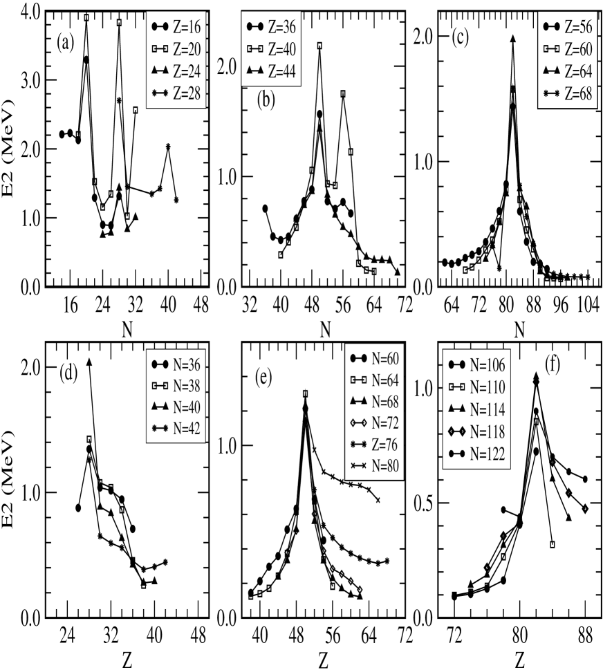
Figure 1: Known E2 values plotted as isolines for even-even nuclei. Isolines drawn in the graphs (a-c) connect E2 values of various isotopes for Z=16 on wards with varying neutron number N, while the isolines drawn in the graphs (d-f) show the same for isotones for N=36 on wards with varying proton number Z. Other possible isolines are not shown here to avoid clumsiness of the graphs.

For a theoretical justification of the above equation, we use the approximation of expressing E2 as the sum of two different functions $E_{1}(N)$ and $E_{2}(Z)$ as

$${E2[N,Z]}=E_{1}(N)+E_{2}(Z).$$ (2)

The goodness of this simplistic approximation can only be judged from numerical analysis of the resulting equations that follow using the experimental data. Secondly we use the empirical fact [see Fig. 1] that E2s are more or less slowly varying functions of N and Z locally. This assumption however cannot be strictly true at the magic numbers and in regions where deformations drastically change. In fact known E2 values plotted as isolines for isotopes and isotones in Fig. 1, convincingly demonstrate the above aspects in most of the cases. The usual typical bending and kinks at magic numbers like 20, 50, 82 and semi-magic numbers 28 and 40 can be seen as a result of sharply changing deformations. Consequently $E_{1}$ and $E_{2}$ can be written directly proportional to N and Z respectively as

$$E_{1}(N)=\lambda N,\leavevmode\nobreak\ \leavevmode\nobreak\ and\leavevmode\nobreak\ \leavevmode\nobreak\ E_{2}(Z)=\nu Z,$$ (3)

where $\lambda$ and $\nu$ are arbitrary constants and vary from branch to branch across the kinks. Then one can easily see that just by substitution of the above two Eqs. (2,3), the differential Eq. (1) gets directly satisfied. Thus the proposed differential equation for E2 analogous to the B(E2)$\uparrow$ relation in the DEM model gets theoretically justified. However, the differential Eq. (1) has its own limitations, and need not be expected to remain strictly valid across the magic-number nuclei because of the very approximations involved in proving it.

III Derivation of the Recursion Relations in E2

It is always desirable to solve the differential Eq. (1) in order to utilize it for practical applications. Therefore it is necessary to obtain possible recursion relations in E2 for even-even nuclei in (N,Z) space from it. The partial derivatives occurring in this equation at mathematical level are defined for continuous functions. However for finite nuclei, these derivatives are to be evaluated taking the difference of E2 values of neighboring nuclei. Since our interest is to obtain recursion relations for even-even nuclei, we use in the above equation the usual forward and backward definitions for the partial derivatives. These are given by

$$\Bigl{(}{\partial E2/\partial N}\Bigr{)}_{Z} \simeq {1\over 2}\Bigl{[}E2[N+2,Z]-E2[N,Z]\Bigr{]},$$

$$\Bigl{(}{\partial E2/\partial Z}\Bigr{)}_{N} \simeq {1\over 2}\Bigl{[}E2[N,Z+2]-E2[N,Z]\Bigr{]},$$

$$and$$

$$\Bigl{(}{\partial E2/\partial N}\Bigr{)}_{Z} \simeq {1\over 2}\Bigl{[}E2[N,Z]-E2[N-2,Z]\Bigr{]},$$

$$\Bigl{(}{\partial E2/\partial Z}\Bigr{)}_{N} \simeq {1\over 2}\Bigl{[}E2[N,Z]-E2[N,Z-2]\Bigr{]}.$$ (5)

Substitution of the above two pairs of definitions for the derivatives in the differential equation (1) enabled us to derive the following two recursion relations for E2, each connecting three neighboring even-even nuclei. These are

$$E2[N,Z] = {N\over{A-2}}\>E2[N-2,Z]+{Z\over{A-2}}\>E2[N,Z-2],$$ (6)

$$E2[N,Z] = {N\over{A+2}}\>E2[N+2,Z]+{Z\over{A+2}}\>E2[N,Z+2]..$$ (7)

The first recursion relation (6) connects three neighboring nuclei (N,Z), (N-2,Z) and (N,Z-2) while the second one (7) connects (N,Z), (N,Z+2) and (N+2,Z). The first one relates E2 of lower to higher mass nuclei while the second one relates higher to lower mass, and hence they can be termed as the forward and backward recursion relations termed as E2-F and E2-B respectively. Thus depending on the availability of E2 data, one can use either or both of these two relations to obtain the corresponding unknown values of neighboring nuclei.

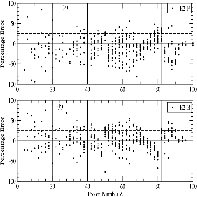
Figure 2: Numerical Test of the Recursion Relations connecting E2 values of neighboring nuclei. The percentage errors of the computed E2 values of all the anchor nuclei are plotted against Proton Number Z of those nuclei. The graph (a) shown as E2-F corresponds to the results of the relation (6) while graph (b) marked as E2-B shows those of the relation (7). The vertical solid lines are drawn just to focus larger deviations if any at the magic and semi-magic numbers.

IV Numerical Test of the Recursion Relations in E2

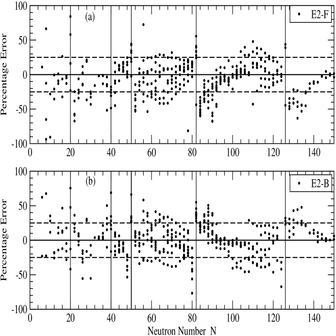
Figure 3: Same as Fig.2 plotted versus Neutron Number N.

Having derived the recursion relations in E2 from the differential equation (III), it is desirable to establish their numerical validity to see to what extent they satisfy the known experimental data throughout the nuclear chart. This would also numerically support the differential equation (1) from which the recursion relations are derived. For this purpose we use the experimentally adopted E2 data set of Raman et al. rmn in the above relations throughout mass range of A=10 to 240 , and compute the same of all possible anchor nuclei that are characterized by the neutron and proton numbers (N,Z) occurring in the left hand sides of the relations (6,7). For better visualization of our results, we calculate the deviations of the computed E2 values from those of the experimental data in terms of the percentage errors following Raman et al. rm2 . The percentage error of a particular calculated quantity is as usual defined as the deviation of that quantity from that of the experiment divided by the average of the concerned data inputs, and then expressed as the percentage of the average. Obviously the larger the percentage error larger is the deviation of the concerned computed value. These percentages so computed are plotted in the figures 2 and 3 against the proton and neutron numbers respectively. This is intentionally done to ascertain to what extent possible deviations occur at proton and neutron magic numbers. From the presented results we see, that in most of the cases both forward and backward recursion relations (6,7) give reasonably good agreement with experiment. Numerically the deviations in 284 out of 417 cases for the forward relation [E2-F] and 278 out of 416 cases for the backward relation [E2-B] lie within $\pm$25% error [shown within broken lines in the figures]. In view of this, the agreement of the model recursion relations with those of experiment can be considered good. However one can see from the figures 2 and 3, that the percentage errors (deviations) are relatively higher for some nuclei in the neighborhood of the magic numbers 20, 50, 82, 126 and semi-magic number 40. Such increase in the vicinity of the magic numbers is expected, as the differential Eq. (1) from which the recursion relations are derived need not be strictly valid at the magic numbers.

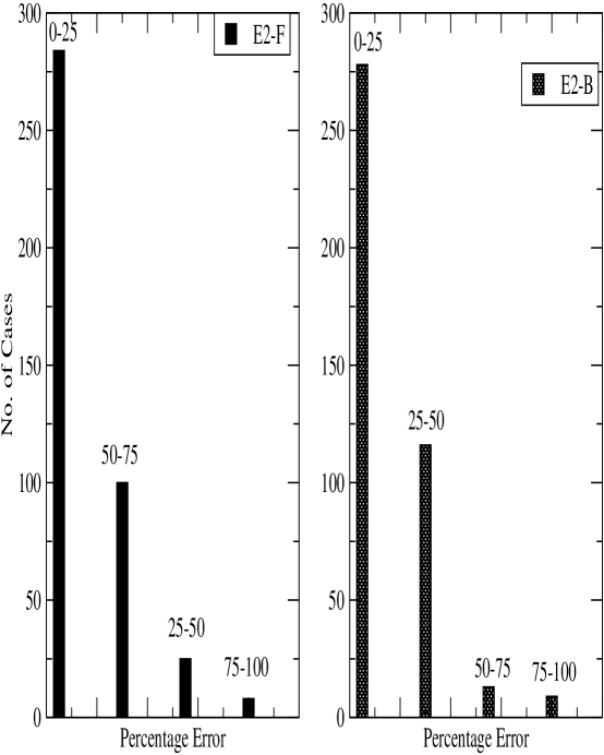
Figure 4: Vertical pillars showing number of cases having different ranges of absolute percentage errors. Those marked as E2-F and E2-B correspond to the results of our relations (6 and 7) respectively.

To bring out the contrasting features of our results in a better way, we also present our results in the form of histograms in Fig. 4, which displays the total number of cases having different ranges of percentage errors. As can be seen, the sharply decreasing heights of the vertical pillars with the increasing range of errors are a clear testimony of the goodness of our recursion relations.

For exact numerical comparison, we also present in Table I results obtained in our calculation along with those of the experiment rmn for some of the nuclides randomly chosen all over the nuclear chart. One can easily see that the agreement of the predictions with the measured values is rather good in most of the cases. In few cases such as ${}^{36}Si$, ${}^{40}S$, ${}^{44}Ca$ and ${}^{220}Rn$ there exists little bit of discrepancy in between the predictions of the relation (7) and those of the experiment. Thus one can fairly say, that the overall agreement of our model predictions with those of experiment is exceedingly good. Therefore such agreement is a clear testimony of the goodness of our recursion relations.

Nucleus	Experiment	B(E2)-B	B(E2)-F	Nucleus	Experiment	B(E2)-B	B(E2)-F
	(MeV)	(MeV)	(MeV)		(MeV)	(MeV)	(MeV)
${}^{24}Ne$	1.982	-	1.782	${}^{30}Mg$	1.482	1.509	1.226
${}^{36}Si$	1.399	2.429	1.104	${}^{40}S$	0.900	1.272	0.969
${}^{44}Ar$	1.144	1.129	1.403	${}^{44}Ca$	1.157	1.447	1.089
${}^{48}Ti$	0.984	1.146	1.152	${}^{74}Ge$	0.596	0.776	0.546
${}^{80}Se$	0.666	0.632	0.689	${}^{82}Kr$	0.776	0.654	0.823
${}^{92}Sr$	0.815	0.798	0.852	${}^{102}Zr$	0.152	0.184	0.158
${}^{106}Mo$	0.172	0.175	0.209	${}^{110}Ru$	0.241	0.227	0.277
${}^{114}Pd$	0.332	0.309	0.403	${}^{120}Cd$	0.506	0.452	0.785
${}^{128}Sn$	1.169	0.965	1.056	${}^{130}Te$	0.839	0.928	0.839
${}^{134}Xe$	0.847	0.803	1.097	${}^{146}Ba$	0.181	0.223	0.146
${}^{148}Ce$	0.159	0.231	0.109	${}^{154}Nd$	0.071	0.077	0.070
${}^{158}Sm$	0.073	0.073	0.072	${}^{160}Gd$	0.075	0.078	0.074
${}^{164}Dy$	0.073	0.078	0.077	${}^{168}Er$	0.080	0.080	0.080
${}^{174}Yb$	0.077	0.079	0.084	${}^{180}Hf$	0.093	0.091	0.098
${}^{186}W$	0.122	0.111	0.146	${}^{192}Os$	0.206	0.196	0.259
${}^{196}Pt$	0.356	0.288	0.405	${}^{202}Hg$	0.438	0.413	0.614
${}^{204}Pb$	0.899	0.759	0.755	${}^{214}Po$	0.609	0.765	0.511
${}^{220}Rn$	0.241	0.401	0.155	${}^{224}Ra$	0.084	0.142	0.069
${}^{232}Th$	0.049	0.055	0.047	${}^{236}U$	0.045	0.046	0.044
${}^{242}Pu$	0.045	0.044	0.046	${}^{246}Cm$	0.043	0.045	0.042
${}^{250}Cf$	0.043	0.043	0.046	${}^{254}Fm$	0.045	0.047	-

Table 1: Comparison of the model predictions referred to as E2-B [Eq. (7)] and E2-F [Eq. (6)] and the experimentalrmn E2 values.

Once we establish the goodness of the two recursion relations, it is desirable to compare our predictions with the latest experimentally adopted data of Pritychenko et al. prt . It must be made clear that none of the values of the new experimental data set has been used in our recursion relations. Rather we use only the available data set of Raman et al. rmn to generate all possible values of a given nucleus employing the two recursions relations (6) and (7). One should note here that each of these relations can be rewritten in three different ways just by shifting the three terms occurring in them from left to right and vice-verse. Thus altogether, these two relations in principle can generate up to six alternate values for a given nucleus subject to availability of the corresponding data. Since each of the values is equally probable, the predicted value for a given nucleus is then obtained by the arithmetic mean of all those generated values so obtained. Our predictions here are confined to those isotopes for which measured values were quoted by Pritychenko et al. prt . The predicted values so obtained termed as the DEM values are presented in Table II for various isotopes of Z=24, 26, 28 and 30 along with those of the latest experimental prt data.

Nucleus	Experiment prt	DEM	Nucleus	Experiment prt	DEM
	(MeV)	(MeV)		(MeV)	(MeV)
${}^{46}Cr$	0.892	0.964	${}^{48}Cr$	0.752	0.723
${}^{50}Cr$	0.783	0.870	${}^{52}Cr$	1.434	1.312
${}^{54}Cr$	0.835	0.977	${}^{56}Cr$	1.007	0.793
${}^{58}Cr$	0.881	0.997	${}^{48}Fe$	0.970	0.805
${}^{50}Fe$	0.765	0.817	${}^{52}Fe$	0.850	0.752
${}^{54}Fe$	1.408	1.476	${}^{56}Fe$	0.847	0.645
${}^{58}Fe$	0.811	0.664	${}^{54}Ni$	1.392	2.078
${}^{56}Ni$	2.701	2.023	${}^{58}Ni$	1.454	1.412
${}^{60}Ni$	1.336	1.222	${}^{62}Ni$	1.173	1.140
${}^{64}Ni$	1.348	1.123	${}^{66}Ni$	1.425	1.431
${}^{68}Ni$	2.034	1.133	${}^{70}Ni$	1.260	1.611
${}^{72}Ni$	1.096	1.111	${}^{74}Ni$	1.024	0.548
${}^{76}Ni$	0.992	0.890	${}^{62}Zn$	0.954	0.918
${}^{64}Zn$	0.992	0.929	${}^{66}Zn$	1.039	1.065
${}^{68}Zn$	1.077	0.832	${}^{70}Zn$	0.885	1.2336
${}^{72}Zn$	0.653	0.717	${}^{74}Zn$	0.606	0.592
${}^{76}Zn$	0.599	0.664	${}^{78}Zn$	0.730	0.645
${}^{80}Zn$	1.492	1.572

Table 2: Comparison of the model predictions and the latest experimental prt E2 values.

We also present our DEM predictions in Fig. 5 to convey a better visualization of our results. One can easily see that in all the cases except for ${}^{54,68,74}Ni$ and ${}^{68,70}Zn$, the agreement between the predictions with those of the experiment are remarkably good. For these few nuclei, the discrepancies may be attributed to the possible sub-shell effect as either proton or neutron numbers or both are close to semi-magic numbers 28 and 40. For sake of comparison we have also presented in Fig. 5, results obtained from two shell-model calculations gxp ; prt marked here as SM1 and SM2. One should note here, that the first one obtained using the effective interactions GXPF1A gxp did not succeed in getting reliable values for nuclei having neutron number beyond N=36 because of its own limitations. Hence the second shell-model with JUN45 effective interaction was performed by Pritychenko et al. prt for the nuclei ${}^{64}Fe,^{68}Ni$ and ${}^{72,74}Zn$. One can easily see that the shell-model values SM1 almost agree with those of ours for almost all the isotopes while the other shell-model values SM2 are rather away from ours as well as from the experimental values.

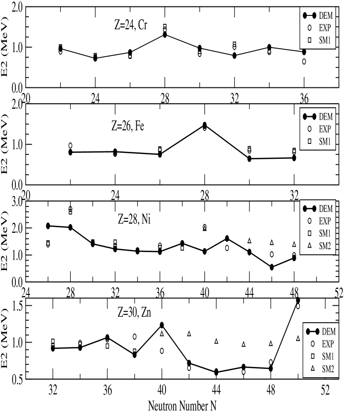
Figure 5: Both calculated (DEM) and the latest experimental (EXP) prt E2 values [see text for details] are presented for various isotopes of Z=24, 26, 28 and 30 versus Neutron Numbers N. DEM Values for different isotopes are connected by solid lines just to guide the eye. Recent shell-model calculated values [SM1 and SM2] are also presented for sake of comparison

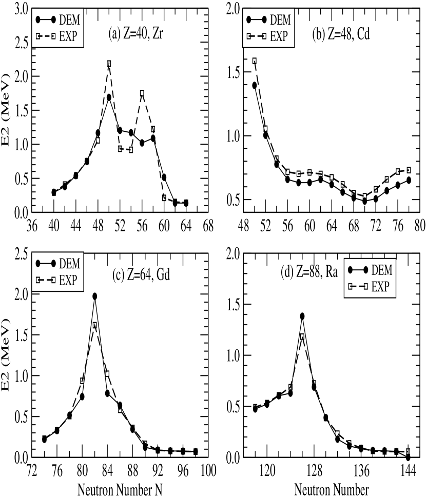
Figure 6: Similar to Fig. 5 but for Z=40, 48, 64 and 88. The experimental data points marked as EXP correspond to those of Raman et al. rmn .

We have just demonstrated as shown above the utility of the recursion relations for predicting E2 values for some of the even-even isotopes of Cr, Fe, Ni and Zn in agreement with the latest experimental prt data. Therefore it is desirable to find out whether the model is good enough for such predictions in the higher mass regions of the nuclear chart. However in these regions there is no new data to compare with and hence we can only compare with the data set of Raman et al. rmn . With this view, we repeated our calculations for higher isotope series following the same methodology outlined above. Since the main aim of our present investigation is just to establish the goodness of our model, we present here results of only few such series for which experimental data exist for a relatively large number of isotopes. Accordingly we have chosen four isotope series Z=40, 48, 64 and 88 covering nuclei both in mid-mass and heavy-mass regions. Our choice of the first two series namely Z=40 and 48 is again to see to what extent our model works across the semi-magic number 40 and magic number 50. Our predictions along with those of experimental data of Raman et al. rmn are presented in Fig. 6. From the presented results we see that the agreement of the model values with experiment is remarkably good. All isotopic variations of our model predictions clearly follow those of the experiment. However small discrepancies exist at the magic numbers N=50, 82 and 126 as the DEM model need not be expected to hold good.

Now taking stock of all the results discussed so far, one can fairly say that the recursion relations for E2 work exceedingly well almost throughout the nuclear chart. Even across the magic numbers and sharply changing deformations, these relations have succeeded in reproducing the experimental data to a large extent with a little bit of deviation here and there. In a nutshell, the recursion relations for the excitation energies E2 derived here can be termed sound enough as to have passed the numerical test both in reproducing and predicting the experimental data , and thereby establish the goodness of the differential equation (1) from which they originate.

V Concluding Remarks

In conclusion, we would like to say that we have succeeded in obtaining for the first time, a novel relation for the first $0_{1}^{+}\rightarrow 2_{1}^{+}$ state excitation energy E2 of a given even-even nucleus in terms of its derivatives with respect to neutron and proton numbers. We could establish such a differential equation on the basis of one-to-one correspondence with the local energy of the Infinite Nuclear Matter model of atomic nuclei and the recently developed Differential Equation Model for the complementary physical quantity B(E2)$\uparrow$. We have also succeeded in establishing its theoretical foundation on the basis of the empirical fact that E2’s are more or less slowly varying functions of neutron and proton numbers except across the magic numbers. We further used the standard definitions of the derivatives with respect to neutron and proton numbers occurring in the equation, to derive two recursion relations in E2. Both these relations are found to connect three different neighboring even-even nuclei from lower to higher mass and vice-verse. The numerical validity of these two relations was further established using the known experimental data set compiled by Raman et al. rmn throughout the mass range of A=10 to 240. More importantly their utility was further demonstrated by comparing our predictions with the latest experimental data set of Pritychenko et al. prt for the isotopes of Cr, Fe, Ni and Zn. The results so obtained convincingly show the goodness of the recursion relations in E2 and thereby their parent differential equation.

99

References

- (1) S. Raman, C. W. Nestor, Jr, P. Tikkanen, At. Data and Nucl. Data Tables 78(2001)1-128
- (2) S. Raman, C. H. Malarkey, W. T. Milner, C. W. Nestor Jr., At. Data and Nucl. Data Tables 36(1987)1.
- (3) B. Pritychenko, J. Choquette, M. Horoi, B. Karamy and B. Singh , At. Data and Nucl. Data Tables 98(2012)798-811
- (4) G. T. Garvey and I. Kelson, Phys. Rev. Lett. 16 (1966) 197
- (5) C. K. Ross and R. K. Bhaduri, Nucl. Phys. A 196 (1972)369
- (6) R. Patnaik, R. Patra and L. Satpathy, Phys. Rev.C12 (1975) 2038
- (7) S. Pattnaik and R. C. Nayak, Int. Jou. of Mod. Phys. E23 (2014) 1450022
- (8) L. Satpathy, J.Phys.G13(1987) 761
- (9) L. Satpathy and R. C. Nayak , At. Data and Nucl. Data Tables 39 (1988) 213
- (10) R. C. Nayak and L. Satpathy, Atom. Data and Nucl. data Tables 73 (1999)213
- (11) R. C. Nayak and L. Satpathy, Atom. Data and Nucl. Data Tables 98 (2012)616
- (12) R. C. Nayak, Phys. Rev.C 60 (1999) 064305
- (13) S. Raman, J. A. Sheikh and K. H. Bhatt, Phys. Rev.C 52 (1995) 1380
- (14) H. Monna, T. Otsuka, B. A. Brown, T. Mizusaki, Eur. Phys. J., A25 (Suppl. 1) (2005)499.
- (15) H. Monna, T. Otsuka, T. Mijusaki, M. Hojorth-Jensen, Phys. Rev. C 80 (2009)064323.
- (16) S. Raman, C. W. Nestor, K. H. Bhatt, Phys. Rev. C 37(1988) 805
99