Design of Efficient Sampling Methods on Hybrid Social-Affiliation Networks
Technique Report

Abstract

Graph sampling via crawling has become increasingly popular and important in the study of measuring various characteristics of large scale complex networks. While powerful, it is known to be challenging when the graph is loosely connected or disconnected which slows down the convergence of random walks and can cause poor estimation accuracy.

In this work, we observe that the graph under study, or called target graph, usually does not exist in isolation. In many situations, the target graph is related to an auxiliary graph and an affiliation graph, and the target graph becomes well connected when we view it from the perspective of these three graphs together, or called a hybrid social-affiliation graph in this paper. When directly sampling the target graph is difficult or inefficient, we can indirectly sample it efficiently with the assistances of the other two graphs. We design three sampling methods on such a hybrid social-affiliation network. Experiments conducted on both synthetic and real datasets demonstrate the effectiveness of our proposed methods.

I Introduction

Online social networks (OSNs) such as Facebook, Sina Weibo, and Twitter have attracted researchers’ much attention in recent years because of their ever-increasing popularity and importance in our daily lives [26, 34, 23, 17, 4]. An OSN not only provides a platform for people to connect with their friends, but also provides an opportunity for researchers to study user characteristics, which are valuable for applications such as marketing decision making. For example, Twitter users’ tweeting activities (e.g., number of tweets related to a movie) can be used to predict movie box-office revenues [5], and Twitter users’ mood characteristics have a relation with stock market prices [9]. Therefore, measuring user characteristics in OSNs is an important task.

Exactly calculating user characteristics requires the complete OSN data. However, for third parties who do not own the data can only rely on public APIs to crawl the OSN. To protect user privacy, OSNs usually impose barriers to limit third parties’ large-scale crawling [25] and restrict the rate of requesting APIs (e.g., Sina Weibo allows a user to issue at most 150 requests per hour [2]). As a result, crawling the complete data of a large-scale OSN is practically impossible.

To address this challenge, sampling methods are developed, i.e., a small fraction of OSN users are sampled and used to calculate the characteristics. In the literature, random walk based sampling methods have become popular [20, 21, 13]. A random walker starts from an initial node in the OSN, and randomly selects a neighbor to visit at the next step; this process repeats until the sampling budget is exhausted. The random walk sampling can generate Markov chain samples which are able to provide unbiased estimates of graph statistics [22].

Motivation: If a graph has community structure, the random walk will suffer from slow mixing, i.e., requiring a long burning period to reach the steady state, which results in a substantially large number of samples so as to keep estimation accuracy. Recent studies have found that the mixing time in several real-world networks is much longer than expected [24]. To overcome the slow mixing problem, one effective approach is to allow the random walker(s) to randomly jump to (or start from) different regions of a network, such as random walk with jumps (RWwJ) [6, 28] and Frontier sampling (FS) [27]. These methods explicitly or implicitly assume that random vertex sampling is enabled. For example, in RWwJ, the walker can randomly jump to other nodes while walking, and the initializing step in FS relies on uniform vertex sampling. However, random vertex sampling can be resource-intensive when the effective account ID space is very sparsely populated such as the following example.

Example 1.

A restaurant company wants to build a new chain store in one of two small candidate cities in China. A market surveyor is sent to study the consuming ability of citizens there. Since most citizens use the check-in service [1] to share their consuming information in Weibo, the surveyor decides to use Weibo as a platform to conduct his research. He plans to uniformly sample two collections of Weibo users in the two cities respectively. It is known that every Weibo account ID consists of ten digits ranging from “1000000000” to the maximum. He generates random numbers in this range as test IDs and finds that about $11\%$ of the test IDs are valid Weibo users. However, because the population sizes of the two cities are small (e.g., hundreds of thousands of citizens comparing to the hundreds of millions of Weibo users), the valid users falling into the two cities has probability as small as $0.1\%$.

In the above example, an effective test ID must fall into one of the two cities, and random vertex sampling becomes extremely inefficient because the probability that a test ID is effective equals $P(\textit{ID is valid})\times P(\textit{ID falls into one city})$, where $P(\textit{ID is valid})\approx 0.11$ and $P(\textit{ID falls into one city})\approx 10^{-3}$. This results in that the surveyor needs to try $10^{4}$ times on average to obtain a valid ID falling in one of the two cities. To make matters worse, in some OSNs such as Pinterest, account IDs are arbitrary-length strings, which makes random vertex sampling practically impossible. So, how can we sample vertex randomly in an OSN when random vertex sampling is extremely inefficient or impractical at all?

Present Work: In Example 1, the key problem is how to effectively sample Weibo users within the two cities. We notice that the check-ins shared by users often contain the venue information, e.g., in which restaurant the user lunched, and most such OSNs (e.g., Foursquare) provide APIs for querying venues (e.g., restaurants) within an area of interest by specifying a rectangle region with the bottom-left and top-right corners latitude-longitude coordinates given, or a circle region with the center point latitude-longitude coordinate and radius given. This function can be used to design efficient sampling methods for sampling venues on a map [18, 19, 31]. Since we can sample venues within an area easily, we are able to indirectly sample Weibo users in an area by relating users to venues through check-in relationships between them. This will be more efficient than directly sampling users in an area. We leave the detailed design of this sampling method in Section III and evaluate it in Section IV.

More than solving a particular problem in Example 1, we are inspired to study a more generalized problem. If we consider the venues in Example 1 as another type of nodes besides user nodes, we can build three graphs, i.e., (1) a user graph formed by users and their relationships, (2) a venue graph formed by venues and their relationships (the edge set can be empty as in Example 1), and (3) a bipartite graph formed by users, venues and their check-in relationships. What we learned from Example 1 is that, when directly sampling the user graph is very difficult or extremely inefficient, we can try to sample the venue graph (which is easier as in Example 1), and the bipartite graph acts as a bridge to connect them. This approach facilitates us to sample user graph indirectly but efficiently. Because the affiliation relationship between users and venues plays an important role in these graphs, we refer to the three graphs as a hybrid social-affiliation network jointly. The formal definition of hybrid social-affiliation network will be given in Section II, and the detailed design of sampling methods on hybrid social-affiliation networks will be depicted in Section III.

Contributions: Overall, we have three main contributions:

• (Problem Novelty) We define the idea of hybrid social-affiliation network and formulate a sampling problem over it. (Section II).

• (Solution Novelty) We design three efficient sampling methods over such a network. These methods facilitate us to indirectly sample a graph efficiently when directly sampling it is difficult (Section III).

• We conduct extensive experiments to validate the proposed methods over both synthetic and real-world networks (Section IV).

II Problem Formulation

In this section, we first define the graph characteristics that we want to measure in this work, and then formally define the hybrid social-affiliation network along with the sampling problem over it.

II-A Graph Characteristics

We model an OSN by an undirected graph $G(\mathcal{U},\mathcal{E})$, where $\mathcal{U}$ and $\mathcal{E}$ are the sets of users and relations among users, respectively. Users in $G$ are labeled. Let $\mathcal{L}=\{l_{1},\ldots,l_{W}\}$ be a set of user labels of size $W$. We map each user $u\in\mathcal{U}$ to a subset of labels he owned by a set function called characteristic function $L\colon\mathcal{U}\mapsto 2^{\mathcal{L}}$. For example, if $\mathcal{L}=\{\text{male},\text{female}\}$, then $L(u)$ represents the gender of $u$.

In many applications, we are interested in measuring the fractions of users having some labels, e.g., the fraction of male/female customers buying a product. This can be represented by the label distribution $\theta=\{\theta_{l}\}_{l\in\mathcal{L}}$, where $\theta_{l}$ is the fraction of users with label $l$. That is

$$\theta_{l}=\frac{1}{n}\sum_{u\in\mathcal{U}}\mathbf{1}\left\{l\in L(u)\right\},\quad l\in\mathcal{L},$$

where $n=|\mathcal{U}|$ is the size of graph $G$, and $\mathbf{1}\left\{\cdot\right\}$ is the indicator function. When the graph size $n$ is known or can be estimated [16, 15], we can also obtain the absolute volume of users having a label $l$ by $n\theta_{l}$.

With this definition of graph characteristics, the objective of sampling then becomes how to collect samples (i.e., nodes) from graph $G$ and design estimators to estimate parameters $\{\theta_{l}\}_{l\in\mathcal{L}}$ based on these samples.

II-B Hybrid Social-Affiliation Networks

Example 1 motivates us to define a hybrid social-affiliation network when directly sampling graph $G$ is difficult or inefficient. A hybrid social-affiliation network consists of three graphs: $G(\mathcal{U},\mathcal{E})$, $G^{\prime}(\mathcal{V},\mathcal{E}^{\prime})$, and $G_{b}(\mathcal{U},\mathcal{V},\mathcal{E}_{b})$, where $\mathcal{U},\mathcal{V}$ are sets of nodes and $\mathcal{E},\mathcal{E}^{\prime},\mathcal{E}_{b}$ are sets of edges. In detail,

• $G(\mathcal{U},\mathcal{E})$ is the target graph whose characteristics $\theta$ are of interest and need to be measured, e.g., the user social network in Example 1.

• $G^{\prime}(\mathcal{V},\mathcal{E}^{\prime})$ is an auxiliary graph which can be sampled more easily or efficiently than sampling the target graph, e.g., the venue graph (with $\mathcal{E}^{\prime}=\emptyset$) in Example 1.

• $G_{b}(\mathcal{U},\mathcal{V},\mathcal{E}_{b})$ is an affiliation graph [33, Chapter 8] which is a bipartite graph connecting nodes in the target and auxiliary graphs, e.g., the graph formed by users, venues and their check-in relationships in Example 1.

Figure 1: An illustration of a hybrid social-affiliation network. The target graph together with auxiliary and affiliation graphs form a better connected graph than target graph itself, which improves sampling efficiency.

An example of such a hybrid social-affiliation network is given in Fig. 1. In addition to Example 1, many other measuring problems can be formed as a hybrid social-affiliation network sampling problem. As another case, let us consider the following example.

Example 2.

Mtime.com [3] is an online movie database in China. Users in Mtime can follow each other to form a social network. Moreover, a user can follow movie actors if he is a fan of the actor. The movie actors can also form connections if they cooperated in a same movie.

In Example 2, if we want to measure the characteristics of the graph formed by Mtime users, and directly sampling users is inefficient (because of the community structure formed by user interests difference, geographic constraints etc., which make the user graph not well connected) we can build a hybrid social-affiliation network as follows:

• The target graph is formed by Mtime users and their following relationships.

• The auxiliary graph is formed by actors and their cooperation relationships.

• The affiliation graph is formed by Mtime users and actors and the fan relationships between them.

Other than the ordinary people, movie actors especially pop stars are more easily to form connections since they have more chances to join same events such as Oscar and Cannes. That is, the auxiliary graph is more likely to be well connected than the target graph. We can leverage this feature to design efficient sampling methods to measure target graph characteristics.

III Sampling Design on Hybrid Social-Affiliation Networks

In this section, we design three sampling methods for measuring target graph characteristics on a hybrid social-affiliation network. The notations that will be used in this section are summarized in Table I.

TABLE I: Notations

$G,G^{\prime},G_{b}$	target/auxiliary/affiliation graph.
$\mathcal{U},\mathcal{V}$	sets of nodes.
$n,n^{\prime}$	size of target/auxiliary graph, i.e., $n\!=\!|\mathcal{U}|,n^{\prime}\!=\!|\mathcal{V}|$.
$\mathcal{E},\mathcal{E}^{\prime},\mathcal{E}_{b}$	sets of edges.
$\mathcal{S},\mathcal{S}^{\prime}$	sets of node samples in target and auxiliary graphs.
$B,B^{\prime}$	sampling budgets, i.e., $B=|\mathcal{S}|,B^{\prime}=|\mathcal{S}^{\prime}|$.
$\mathcal{V}_{u},\mathcal{U}_{v}$	neighbors of node $u$ or $v$ in the graph.
$d_{u},d_{v}$	degree of node $u$ (or $v$) in target (or auxiliary) graph.
$d_{u}^{(b)},d_{v}^{(b)}$	degree of node $u$ (or $v$) in affiliation graph.

III-A Indirectly Sampling Target Graph by Vertex Sampling on Auxiliary Graph (VS^A)

When random vertex sampling is more easily to be conducted on auxiliary graph than on target graph such as the case in Example 1, we propose a sampling method VS^A to randomly sample vertices in auxiliary graph so as to indirectly sample target graph. The basic idea of VS^A is illustrated in Fig. 2.

Figure 2: VS^A. Edges in target and auxiliary graphs are omitted.

Suppose a node $v\in\mathcal{V}$ is sampled with probability $p_{v}$ in $G^{\prime}$. For example, when graph $G^{\prime}$ supports the uniform vertex sampling, then $p_{v}=1/n^{\prime},\forall v\in\mathcal{V}$, where $n^{\prime}=|\mathcal{V}|$ is the size of graph $G^{\prime}$.

Sampling Design. The sampling design of VS^A consists of the following two steps:

Step (i)

Sampling a collection of $B^{\prime}$ nodes with replacement in auxiliary graph $G^{\prime}$, and denote these samples by $\mathcal{S}^{\prime}=\{y_{1},\ldots,y_{B^{\prime}}\}$.

Step (ii)

For each $v\in\mathcal{S}^{\prime}$, let $\mathcal{U}_{v}\subseteq\mathcal{U}$ be the subset of nodes that are connected to $v$ in $G_{b}$, and nodes in $\mathcal{U}_{v}$ are all included into $\mathcal{S}$, i.e., $\mathcal{S}=\mathcal{S}\cup\mathcal{U}_{v}$.

Having collected samples $\mathcal{S}$ in the target graph, VS^A uses $S$ to estimate target graph characteristics.

Estimators. When $n=|\mathcal{U}|$ is known in advance, we can use the following estimator to estimate $\theta_{l}$,

$$\hat{\theta}_{l}^{\text{VS\textsuperscript{A}}}=\frac{1}{nB^{\prime}}\sum_{i=1}^{B^{\prime}}\frac{1}{p_{y_{i}}}\sum_{u\in\mathcal{U}_{y_{i}}}\frac{\mathbf{1}\left\{l\in L(u)\right\}}{d_{u}^{(b)}},$$ (1)

where $d_{u}^{(b)}$ is the degree of node $u$ in affiliation graph $G_{b}$. When $n$ is unknown, we can estimate $n$ by

$$\hat{n}=\frac{1}{B^{\prime}}\sum_{i=1}^{B^{\prime}}\frac{1}{p_{y_{i}}}\sum_{u\in\mathcal{U}_{y_{i}}}\frac{1}{d_{u}^{(b)}},$$ (2)

and another estimator for $\theta_{l}$ when $n$ is unknown is

$$\check{\theta}_{l}^{\text{VS\textsuperscript{A}}}=\frac{1}{\hat{n}B^{\prime}}\sum_{i=1}^{B^{\prime}}\frac{1}{p_{y_{i}}}\sum_{u\in\mathcal{U}_{y_{i}}}\frac{\mathbf{1}\left\{l\in L(u)\right\}}{d_{u}^{(b)}}.$$ (3)

The following theorem guarantees the unbiasedness of these estimators.

Theorem 1.

Estimators (1) and (2) are unbiased estimators of $\theta_{l}$ and $n$, respectively. Estimator (3) is an asymptotically unbiased estimator of $\theta_{l}$.

Proof.

We show that

$$\mathbb{E}\left[\hat{\theta}_{l}^{\text{VS\textsuperscript{A}}}\right] =\frac{1}{nB^{\prime}}\sum_{i=1}^{B^{\prime}}\mathbb{E}\left[\frac{1}{p_{y_{i}}}\sum_{u\in\mathcal{U}_{y_{i}}}\frac{\mathbf{1}\left\{l\in L(u)\right\}}{d_{u}^{(b)}}\right]$$

$$=\frac{1}{n}\sum_{v\in\mathcal{V}}p_{v}\frac{1}{p_{v}}\sum_{u\in\mathcal{U}_{v}}\frac{\mathbf{1}\left\{l\in L(u)\right\}}{d_{u}^{(b)}}$$

$$=\frac{1}{n}\sum_{u\in\mathcal{U}}\mathbf{1}\left\{l\in L(u)\right\}$$

$$=\theta_{l}.$$

The second equality holds because that $y_{i},i=1,\ldots,B^{\prime}$ are i.i.d random variables. The third equality holds because that each item in the inner summation is added $d_{u}^{(b)}$ times for each $u\in\mathcal{U}$. Hence, $\hat{\theta}_{l}^{\text{VS\textsuperscript{A}}}$ is unbiased.

In a similar manner, we can prove that estimator (2) is an unbiased estimator of $n$, which we omit here.

To prove that estimator (3) is asymptotically unbiased, we use the ratio form of the law of large numbers in [22, Theorem 17.2.1 on P. 428]. Hence

$$\lim_{B^{\prime}\rightarrow\infty}\check{\theta}_{l}^{\text{VS\textsuperscript{A}}}=\frac{\mathbb{E}\left[n\hat{\theta}_{l}^{\text{VS\textsuperscript{A}}}\right]}{\mathbb{E}\left[\hat{n}\right]}=\theta_{l}.$$

∎

It is important to note that VS^A can only sample nodes in $\mathcal{U}$ satisfying $d_{u}^{(b)}>0$ in the target graph. Because a node in $G$ having no connection to nodes in $G^{\prime}$ can not be indirectly sampled according to the design of VS^A. In Example 1, since we are only interested in users who have check-ins in Weibo, therefore Example 1 satisfies this condition.

III-B Random Walking on Target Graph with Vertex Sampling on Auxiliary Graph (RW^TVS^A)

In some situations, $d_{u}^{(b)}=0$ for some $u\in\mathcal{U}$. For example, some user nodes in Example 2 may not follow any movie actors at all, and these users cannot be sampled by VS^A. To overcome this problem, we design another sampling method RW^TVS^A which combines random walk sampling on target graph and vertex sampling on auxiliary graph.

The basic idea of RW^TVS^A is that, we run a simple random walk on the target graph, and at each step the random walk jumps with a probability related to the node that it currently resides. The node to jump to is randomly chosen from neighbors of $v$ in the affiliation graph and $v$ is randomly sampled in the auxiliary graph. We can show that this approach is equivalent to the standard RWwJ [6, 28] on $G$, and this idea is illustrated in Fig. 3. An additional advantage of running random walk on target graph is that a random walk can better characterize highly connected nodes than uniform sampling as random walks are biased to sample high degree nodes in $G$.

Figure 3: RW^TVS^A. Edges in target and auxiliary graphs are omitted.

As in VS^A, we assume a node $v\in\mathcal{V}$ can be sampled with probability $p_{v}$. In RW^TVS^A, we virtually connect each node $u\in\mathcal{U}$ to a jumper node $j$ by edge $(u,j)$, and each edge $(u,j)$ is assigned with a weight $\omega_{u}=\alpha q_{u}$, where $\alpha$ is a constant controlling the probability of jumping at each step of random walk, and $q_{u}$ is determined as follows in order to protect the reversible property of Markov chain.

$$q_{u}=\sum_{v\in\mathcal{V}_{u}}\frac{p_{v}}{d_{v}^{(b)}},\ u\in\mathcal{U},$$ (4)

where $\mathcal{V}_{u}$ is the subset of nodes in $\mathcal{V}$ that are connected to $u$, and $d_{v}^{(b)}$ is the degree of node $v$ in affiliation graph $G_{b}$. The random walk jumps from a node $u$ to jumper $j$ with probability

$$p_{uj}=\frac{\omega_{u}}{d_{u}+\omega_{u}},$$

and moves from the jumper $j$ to $u$ with probability

$$p_{ju}=\frac{\omega_{u}}{\sum_{u^{\prime}}\omega_{u^{\prime}}}=q_{u}.$$

Note that, if $d_{u}^{(b)}=0$, then $p_{uj}=p_{ju}=0$ according to Eq. (4). So the random walk does not jump from $u$ or to $u$ if $d_{u}^{b}=0$.

RW^TVS^A exhibits similar properties as RWwJ. That is, when $\alpha=0$, RW^TVS^A becomes a simple random walk on the target graph. When $\alpha=\infty$, RW^TVS^A is equivalent to VS^A and it is also equivalent to random vertex sampling on the target graph with probability distribution $\{q_{u}\}_{u\in\mathcal{U}}$.

When RW^TVS^A reaches the steady state, each node $u$ is sampled with probability

$$\pi_{u}=\frac{d_{u}+\omega_{u}}{2|\mathcal{E}|+\alpha},\ u\in\mathcal{U}.$$ (5)

Sampling Design. Suppose the random walk starts at node $x_{1}\in\mathcal{U}$, and at step $i$ the random walker is at node $x_{i}$. We calculate the probability $q_{x_{i}}$ according to Eq. (4) and $\omega_{x_{i}}=\alpha q_{x_{i}}$. At step $i$, the walker jumps with probability $\omega_{x_{i}}/(d_{x_{i}}+\omega_{x_{i}})$; otherwise, the walker moves to a neighbor $u$ of $x_{i}$ chosen uniformly at random and set $x_{i+1}=u$. The jump is conducted as follows:

Step (i)

We sample a node $v\in\mathcal{V}$ in the auxiliary graph with probability $p_{v}$.

Step (ii)

We sample a neighbor $u$ of $v$ uniformly at random in the affiliation graph, and let $x_{i+1}=u$.

Estimator. According to the stationary distribution Eq. (5) of RW^TVS^A, we can use the sample path $\{x_{i}\}_{i=1}^{B}$ by the random walk to design a Hansen-Hurwitz estimator of $\{\theta_{l}\}_{l\in\mathcal{L}}$ as follows,

$$\hat{\theta}_{l}^{\text{RW\textsuperscript{T}}\text{VS\textsuperscript{A}}}=\frac{1}{Z}\sum_{i=1}^{B}\frac{\mathbf{1}\left\{l\in L(x_{i})\right\}}{d_{x_{i}}+\omega_{x_{i}}},$$ (6)

where $Z=\sum_{i=1}^{B}1/(d_{x_{i}}+\omega_{x_{i}})$.

Theorem 2.

Estimator (6) is an asymptotically unbiased estimator of $\theta_{l}$.

Proof.

Let $D\triangleq\sum_{i=1}^{B}\mathbf{1}\left\{l\in L(x_{i})\right\}/(d_{x_{i}}+\omega_{x_{i}})$. Then

$$\mathbb{E}\left[D\right] =B\mathbb{E}\left[\frac{\mathbf{1}\left\{l\in L(x_{i})\right\}}{d_{x_{i}}+\omega_{x_{i}}}\right]$$

$$=B\sum_{u\in\mathcal{U}}\pi_{u}\frac{\mathbf{1}\left\{l\in L(u)\right\}}{d_{u}+\omega_{u}}$$

$$=\frac{B}{2|\mathcal{E}|+\alpha}\sum_{u\in\mathcal{U}}\mathbf{1}\left\{l\in L(u)\right\}$$

$$=\frac{Bn}{2|\mathcal{E}|+\alpha}\theta_{l}.$$

Similarly, we can show that

$$\mathbb{E}\left[Z\right] =\mathbb{E}\left[\sum_{i=1}^{B}\frac{1}{d_{x_{i}}+\omega_{x_{i}}}\right]$$

$$=B\mathbb{E}\left[\frac{1}{d_{x_{i}}+\omega_{x_{i}}}\right]$$

$$=B\sum_{u\in\mathcal{U}}\pi_{u}\frac{1}{d_{u}+\omega_{u}}$$

$$=\frac{Bn}{2|\mathcal{E}|+\alpha}.$$

Now, we invoke Theorem 17.2.1 in [22, P. 428], which is the ratio form of the law of large numbers, and indicate that

$$\lim_{B\rightarrow\infty}\hat{\theta}_{l}^{\text{RW\textsuperscript{T}}\text{VS\textsuperscript{A}}}=\frac{\mathbb{E}\left[D\right]}{\mathbb{E}\left[Z\right]}=\theta_{l}.$$

∎

Note that RW^TVS^A requires that we can conduct vertex sampling on auxiliary graph $G^{\prime}$. In fact, we can replace vertex sampling by another simple random walk on auxiliary graph $G^{\prime}$. However, this simple random walk may be easily trapped when $G^{\prime}$ is not well connected. In the follows, we design a new method to address this problem.

III-C Random Walking on Target Graph with Random Walking on Auxiliary Graph (RW^TRW^A)

When both the target and auxiliary graphs do not support random vertex sampling, neither VS^A nor RW^TVS^A can be applied under this situation. Therefore, we design the RW^TRW^A method in this subsection, namely, random walking on the target graph with random walking on the auxiliary graph. RW^TRW^A consists of two parallel random walks on $G$ and $G^{\prime}$ respectively. The two parallel random walks cooperate with each other, and can be considered as two random walks with jumps, as illustrated in Fig. 4. Nodes in $G$ and $G^{\prime}$ are virtually connected to two jumper nodes $j_{1}$ and $j_{2}$, respectively.

Figure 4: RW^TRW^A. Edges in target and auxiliary graphs are omitted.

The basic idea behind RW^TRW^A is as follows. Suppose the two random walks are $RW$ on $G$ and $RW^{\prime}$ on $G^{\prime}$ respectively, and they are at $x_{i}$ and $y_{i}$ at step $i$. If one random walk needs to jump at step $i$, say $RW$, then the node to jump to is randomly chosen from $y_{i}$’s neighbors in the affiliation graph and assigned to $x_{i+1}$. Similar jumping procedure also applies to $RW^{\prime}$. Therefore, they are equivalent to two RWwJs.

The main problem we need to solve is how to determine edge weights $\omega_{\mathcal{U}}\triangleq\{\omega_{u}\}_{u\in\mathcal{U}}$ and $w_{\mathcal{V}}\triangleq\{w_{v}\}_{v\in\mathcal{V}}$, which control the probability of jumping on $G$ and $G^{\prime}$ respectively. Obviously, the stationary distributions of the two random walks are related to these weights. Let $\pi_{u}$ and $\pi_{v}$ be the stationary distributions of sampling nodes in $G$ and $G^{\prime}$ respectively. They are determined by

$$\pi_{u} =\frac{d_{u}+\omega_{u}}{2|\mathcal{E}|+\alpha},\ u\in\mathcal{U},$$ (7)

$$\pi_{v} =\frac{d_{v}+w_{v}}{2|\mathcal{E}^{\prime}|+\beta},\ v\in\mathcal{V},$$ (8)

where $\alpha$ and $\beta$ are two constants. These weights should be assigned properly so as to keep the reversibility of Markov chains. Therefore, stationary distributions control $\omega_{u}$ and $w_{v}$ in turn.

$$\omega_{u} =\alpha\sum_{v\in\mathcal{V}_{u}}\frac{\pi_{v}}{d_{v}^{(b)}},\ u\in\mathcal{U},$$ (9)

$$w_{v} =\beta\sum_{u\in\mathcal{U}_{v}}\frac{\pi_{u}}{d_{u}^{(b)}},\ v\in\mathcal{V}.$$ (10)

Or we can arrange Eqs. (7)-(10) in matrix formulas,

$$\pi_{\mathcal{U}} =\frac{d_{\mathcal{U}}+\omega_{\mathcal{U}}}{2|\mathcal{E}|+\alpha}, \pi_{\mathcal{V}} =\frac{d_{\mathcal{V}}+w_{\mathcal{V}}}{2|\mathcal{E}^{\prime}|+\beta},$$

$$\omega_{\mathcal{U}} =\alpha AD_{\mathcal{V}}^{-1}\pi_{\mathcal{V}}, w_{\mathcal{V}} =\beta A^{T}D_{\mathcal{U}}^{-1}\pi_{\mathcal{U}},$$

where $A=[a_{uv}]_{n\times n^{\prime}}$ is the adjacency matrix of $G_{b}$, $\pi_{\mathcal{U}}=[\pi_{u}]_{u\in\mathcal{U}}^{T},\pi_{\mathcal{V}}=[\pi_{v}]_{v\in\mathcal{V}}^{T}$, $\omega_{\mathcal{U}}=[\omega_{u}]_{u\in\mathcal{U}}^{T},w_{\mathcal{V}}=[w_{v}]_{v\in\mathcal{V}}^{T}$, $d_{\mathcal{U}}=[d_{u}]_{u\in\mathcal{U}}^{T},d_{\mathcal{V}}=[d_{v}]_{v\in\mathcal{V}}^{T}$ are six vectors, and $D_{\mathcal{U}}=diag(d_{u_{1}}^{(b)},\ldots,d_{u_{n}}^{(b)}),D_{\mathcal{V}}=diag(d_{v_{1}}^{(b)},\ldots,d_{v_{n^{\prime}}}^{(b)})$.

Above equations can uniquely determine $\omega_{\mathcal{U}}$ and $w_{\mathcal{V}}$, i.e.,

$$\omega_{\mathcal{U}} \!=\!c^{\prime}(I\!-\!cc^{\prime}AD_{\mathcal{V}}^{-1}A^{T}D_{\mathcal{U}}^{-1})^{-1}\!AD_{\mathcal{V}}^{-1}(d_{\mathcal{V}}\!+\!cA^{T}D_{\mathcal{U}}^{-1}d_{\mathcal{U}}),$$

$$w_{\mathcal{V}} \!=\!c(I\!-\!cc^{\prime}A^{T}D_{\mathcal{U}}^{-1}AD_{\mathcal{V}}^{-1})^{-1}\!A^{T}D_{\mathcal{U}}^{-1}(d_{\mathcal{U}}\!+\!c^{\prime}AD_{\mathcal{V}}^{-1}d_{\mathcal{V}}),$$

where $c=\beta/(2|\mathcal{E}|+\alpha)$ and $c^{\prime}=\alpha/(2|\mathcal{E}^{\prime}|+\beta)$ are two constants.

Above results illustrate that, given $\alpha$ and $\beta$, $\omega_{\mathcal{U}}$ and $w_{\mathcal{V}}$ are uniquely determined. However, they need complete knowledges of $G$, $G^{\prime}$ and $G_{b}$ to determine their precise values. This feature is not suitable for us to design an algorithm that only uses local information of these graphs. In what follows, we address this problem and design RW^TRW^A in a way that only requires local knowledges of these graphs.

Suppose we firstly fix $\omega_{u}=\alpha q_{u}$, e.g., specify $q_{u}$ to follow a uniform distribution over $\mathcal{U}$. Using above equations, we can determine $\pi_{u}$, $w_{v}$ and $\pi_{v}$ in order. Then, using Eq. (9), we can calculate a new $\omega_{u}^{\prime}$ which may not equal to $\omega_{u}$. Let $\omega_{u}^{\prime}=\alpha q_{u}^{\prime}$. Since $q_{u}\neq q_{u}^{\prime}$, this will cause the Markov chain on $G$ to be non-reversible. To address this problem, we apply Metropolis-Hastings sampler [29, Chapter 7] by considering $\{q_{u}\}_{u\in\mathcal{U}}$ as the desired distribution and $\{q_{u}^{\prime}\}_{u\in\mathcal{U}}$ as the proposal distribution. Therefore, we can use Metropolis-Hastings sampler to build a Markov chain (refer as MH chain) that can generate samples with the desired distribution $\{q_{u}\}_{u\in\mathcal{U}}$, and each time when the random walk on $G$ requires to jump, it jumps to a sample of MH chain, thereby preserving the reversibility of Markov chain on $G$.

Input: A desired distribution $\{q_{u}\}_{u\in\mathcal{U}}$, and a proposed distribution $\{q_{u}^{\prime}\}_{u\in\mathcal{U}}$.

Output: A Markov chain with the desired stationary distribution.

1 Let $u_{t}$ be the sample at time $t$;

2 while not stop, do

3       Draw $u$ from $\{q_{u}^{\prime}\}$;

4       Calculate the acceptance ratio $r_{t}=\min\{1,\frac{q_{u}q_{u_{t}}^{\prime}}{q_{u_{t}}q_{u}^{\prime}}\}$;

5       Set $u_{t+1}=u$ with probability $r_{t}$;

6       Set $u_{t+1}=u_{t}$ with probability $1-r_{t}$;

7      

8 end while

Algorithm 1 Metropolis-Hastings Sampler.

Sampling Design. We specify a desired sampling distribution $\{q_{u}\}_{u\in\mathcal{U}}$ over $\mathcal{U}$, e.g., a uniform distribution. The complete sampling design of RW^TRW^A comprises three Markov chains as shown in Fig. 5.

•Random Walk on Auxiliary Graph: Suppose the random walker resides at node $y_{i}\in\mathcal{V}$ at step $i$. Then we can easily calculate $w_{y_{i}}$ according to Eq. (10). At step $i+1$, the walker execute one of the following two steps.

Jumping

With probability $w_{y_{i}}/(d_{y_{i}}+w_{y_{i}})$, the walker jumps to a random neighbor $v\in\mathcal{V}$ of node $x_{i}$ in $G_{b}$, and set $y_{i+1}=v$;

Walking

Otherwise, the walker moves to a random neighbor $v\in\mathcal{V}$ of $y_{i}$ in $G^{\prime}$, and set $y_{i+1}=v$.

•Metropolis-Hastings (MH) Chain: Suppose the MH chain resides at node $x^{\prime}_{i}$ at step $i$. At step $i+1$, we randomly choose a neighbor $u\in\mathcal{U}$ of $y_{i}$ in $G_{b}$. This is equivalent to sample a node $u\in\mathcal{U}$ with probability $q_{u}$.

Accept

With probability $r_{i}$, we accept $u$ and set $x^{\prime}_{i+1}=u$, where $r_{i}=\min\{1,(q_{u}q_{x^{\prime}_{i}}^{\prime})/(q_{x^{\prime}_{i}}q_{u}^{\prime})\}$ (note that $q_{x^{\prime}_{i}}^{\prime}$ has been calculated at step $i$).

Reject

Otherwise, we reject $u$ and set $x^{\prime}_{i=1}=x^{\prime}_{i}$.

•Random Walk on Target Graph: Suppose the random walker resides at node $x_{i}\in\mathcal{U}$ at step $i$. Then we can easily calculate $\omega_{x_{i}}$ according to Eq. (9). At step $i+1$, the walker execute one of the following two steps.

Jumping

With probability $\omega_{x_{i}}/(d_{x_{i}}+\omega_{x_{i}})$, the walker jumps to $x^{\prime}_{i+1}$, and set $x_{i+1}=x^{\prime}_{i+1}$;

Walking

Otherwise, the walker moves to a random neighbor $u\in\mathcal{U}$ of $x_{i}$ in $G$, and set $x_{i+1}=u$.

Figure 5: Markov chains in the RW^TRW^A.

Estimator. We use the sample path $\{x_{i}\}_{i=1}^{B}$ by the random walk on $G$ to design an estimator to estimate $\{\theta_{l}\}_{l\in\mathcal{L}}$ as follows,

$$\hat{\theta}_{l}^{\text{RW\textsuperscript{T}}\text{RW\textsuperscript{A}}}=\frac{1}{Z}\sum_{i=1}^{B}\frac{\mathbf{1}\left\{l\in L(x_{i})\right\}}{d_{x_{i}}+\omega_{x_{i}}},$$ (11)

where $Z=\sum_{i=1}^{B}1/(d_{x_{i}}+\omega_{x_{i}})$.

Theorem 3.

Estimator (11) is an asymptotically unbiased estimator for $\theta_{l}$.

Proof.

First we note that the random walk on target graph $G$ has the same stationary distribution as Eq. (5). So the remaining proof is similar to the proof of Theorem 2. ∎

IV Experiments

In this section, we conduct experiments on both synthetic and real-world datasets to evaluate the effectiveness of proposed methods in previous section. We will use degree distribution as the graph characteristic to be measured in these experiments. That is, $\theta_{l},l\geq 0$ denotes the fraction of nodes with degree $l$ in the target graph $G$.

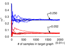
((a)) $\check{\theta}^{\text{VS\textsuperscript{A}}}_{2}$ and $\check{\theta}^{\text{VS\textsuperscript{A}}}_{12}$

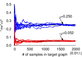
((b)) $\hat{\theta}^{\text{RW\textsuperscript{T}}\text{VS\textsuperscript{A}}}_{2}$ and $\hat{\theta}^{\text{RW\textsuperscript{T}}\text{VS\textsuperscript{A}}}_{12}$ ($\alpha=10$)

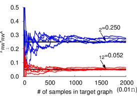
((c)) $\hat{\theta}^{\text{RW\textsuperscript{T}}\text{RW\textsuperscript{A}}}_{2}$ and $\hat{\theta}^{\text{RW\textsuperscript{T}}\text{RW\textsuperscript{A}}}_{12}$ ($\alpha=\beta=10$)

Figure 6: Asymptotic unbiasedness of the estimators ($l=2,12$).

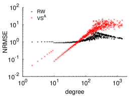
((a)) VS^A

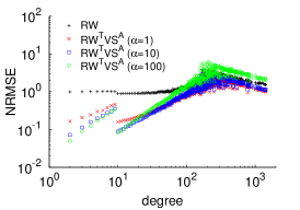
((b)) RW^TVS^A

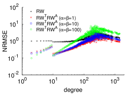
((c)) RW^TRW^A

Figure 7: Estimation error comparison (averaged over $1,000$ runs, $2,000$ samples in target graph).

IV-A Experiments on Synthetic Data

We first examine the soundness of the proposed sampling methods using synthetic data.

Synthetic Data. We generate a hybrid social-affiliation network by connecting three Barabási-Albert graphs [7], namely $G_{1},G_{2}$ and $G_{3}$. Each BA graph contains $100,000$ nodes but they have different average degrees, i.e., $4,10$ and $20$ respectively. $G_{1}$ and $G_{3}$ are connected with one edge to form the target graph $G$. $G_{2}$ is the auxiliary graph $G^{\prime}$. The affiliation graph $G_{b}$ is formed by following two rules:

1. For each node $u$ in $G$, we connect $u$ to a randomly selected node $v$ in $G^{\prime}$;

2. We randomly choose $200,000$ pairs of nodes in $G$ and $G^{\prime}$, and connect them to form edges in $G_{b}$.

The first rule makes sure that every node in $\mathcal{U}$ satisfies $d_{u}^{(b)}>0$. Therefore we can apply VS^A method on the synthetic graph.

Results and Analysis. First we demonstrate that the proposed estimators $\check{\theta}_{l}^{\text{VS\textsuperscript{A}}},\hat{\theta}_{l}^{\text{RW\textsuperscript{T}}\text{VS\textsuperscript{A}}}$ and $\hat{\theta}_{l}^{\text{RW\textsuperscript{T}}\text{RW\textsuperscript{A}}}$ are asymptotically unbiased. To show this, we use different sampling budgets, i.e., number of samples in the target graph, and compare the estimator values with the ground truth. The results are depicted in Fig. 6. We use these sampling methods to estimate $\theta_{2}$ and $\theta_{12}$. As the sampling budget increases, all the estimators converge to the ground truth values, thereby demonstrating their asymptotic unbiasedness.

To compare the performance of proposed sampling methods with existing methods, e.g., a simple random walk (RW) on $G$, we use the normalized rooted mean squared error (NRMSE) to evaluate the estimation error of an estimator, which is defined as follows.

$$\text{NRMSE}(\hat{\theta}_{l})=\frac{\sqrt{\mathbb{E}\left[(\hat{\theta}_{l}-\theta_{l})^{2}\right]}}{\theta_{l}}.$$

The smaller the NRMSE, the better an estimator is. We fix the sampling budget to be $1\%$ of the nodes in target graph, and calculate the averaged empirical NRMSE over $1,000$ runs in Fig. 7.

Comparing VS^A with RW, we find that VS^A can provide smaller NRMSE for low degree nodes than RW. However, VS^A produces larger NRMSE for high degree nodes than RW. Therefore, VS^A can better estimate low degree nodes in a graph but not high degree nodes than the RW estimator.

The weakness of VS^A can be overcome by RW^TVS^A and RW^TRW^A. From Figs. 7(b) and 7(c) we can see that, when we allow jumps in RW^TVS^A and RW^TRW^A by setting $\alpha=\beta=1$, the NRMSE for high degree nodes decreases as small as RW, and NRMSE for low degree nodes keeps smaller than RW. If we increase the probability of jumping at each step by increasing $\alpha$ and $\beta$, we observe that the NRMSE for low degree nodes decreases, and NRMSE for high degree nodes increases. This behavior is similar to RWwJ [6, 28] because RW^TVS^A and RW^TRW^A are equivalent to RWwJ in the design.

IV-B Experiments on LBSN Datasets

Now we conduct experiments on two real-world location-based social network (LBSN) datasets to solve the problem mentioned in Example 1.

LBSN Datasets. We use two public datasets Brightkite and Gowalla [10] to solve our first problem in Example 1. Brightkite and Gowalla are once two popular LBSNs where users shared their locations by checking-in. Users are also connected by undirected friendship relationships. The statistics of the two datasets are summarized in Table II.

TABLE II: Summary of LBSN datasets.

[b] dataset Brightkite Gowalla $G$ network type undirected undirected # of users $58,228$ $196,591$ # of friendship edges $214,078$ $950,327$ # of users in LCC¹ $56,739$ $196,591$ # of edges in LCC $212,945$ $950,327$ $G^{\prime}$ and $G_{b}$ # of distinct venues $772,966$ $1,280,969$ # of users having check-ins $51,406$ $107,092$ # of check-ins $4,491,143$ $6,442,890$ $G^{\prime}$ and $G_{b}$ for NYC # of venues in NYC² $23,484$ $26,448$ # of users checking in NYC $4,257$ $7,399$ # of check-ins in NYC $33,656$ $113,423$

• The largest connected component.

• The New York City (Fig. 8).

Venue Sampling. Suppose the surveyor wants to measure characteristics of users located in New York City (NYC, latitude $40.4^{\circ}\sim 41.4^{\circ}$, longitude $-74.3^{\circ}\sim-73.3^{\circ}$, see Fig. 8), i.e., the degree distribution of users who checked in NYC. As we explained in Introduction, directly sampling users is not a good idea. Here, we apply the VS^A method along with a venue sampling method Random Region Zoom-In (RRZI) [31] to sample users in NYC more efficiently.

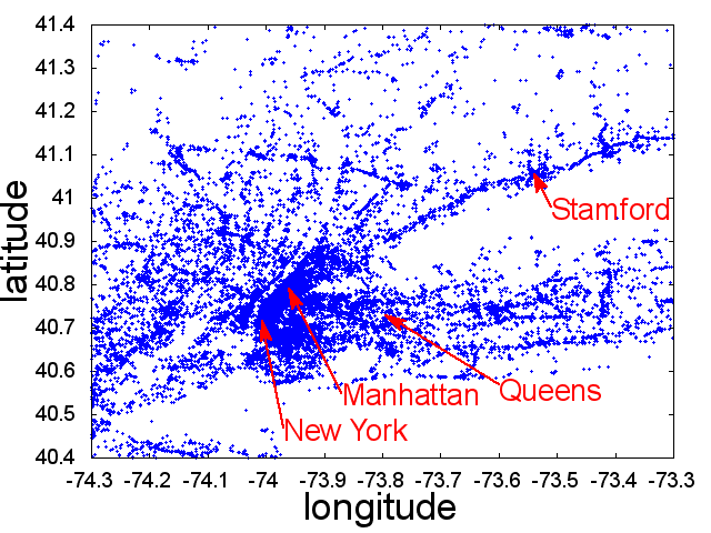
Figure 8: Venue distribution in New York City

RRZI utilizes the venue query API provided by most LBSNs. A user first specifies a region by giving the bottom-left and top-right corner latitude-longitude coordinates, and the API returns a set of venues in this region. Usually, the size of the set returned is limited to at most $K$ if there are more than $K$ venues in the region. RRZI regularly zooms in the region until the subregion is fully accessible, i.e., the API returns less than $K$ venues in the subregion. Therefore, RRZI can provide samples of venues in a region of interest.

Results. Combining the RRZI and VS^A methods, we conduct two experiments to indirectly sample users in NYC on Brightkite and Gowalla respectively. We sample $1\%$ of venues in NYC and calculate the degree distribution of users in NYC. The results are depicted in Figs. 9 and 10.

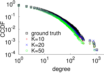
((a)) RRZI-VS^A estimates

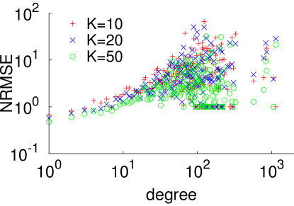
((b)) RRZI-VS^A NRMSE

Figure 9: User characteristics in NYC on Brightkite. (averaged over $1000$ runs)

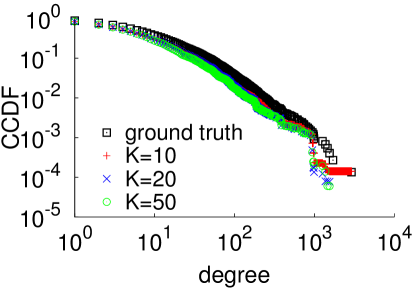
((a)) RRZI-VS^A estimates

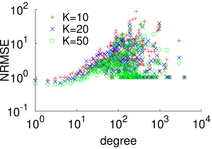
((b)) RRZI-VS^A NRMSE

Figure 10: User characteristics in NYC on Gowalla. (averaged over $1000$ runs)

From Figs. 9(a) and 10(a), we can see that RRZI-VS^A method can provide well estimates of users in NYC, and the estimates for low degree users are better than high degree users, which are clearer from Figs. 9(b) and 10(b). These results are consistent with our previous analysis on synthetic data. In fact, we can combine VS^A with other venue sampling methods [18, 19, 31] to provide better estimates than RRZI. However, we omit them due to space limitation.

IV-C Experiments on Mtime Dataset

Next, we conduct experiments on Mtime to measure Mtime user characteristics in Example 2.

Mtime Dataset. As we have introduced in Example 2, users and actors in Mtime naturally form a hybrid social-affiliation network. To build a ground-truth dataset, we almost completely collected the Mtime users and actors data by traversing user IDs ranging from $100000$ to $10000000$, and actor IDs ranging from $892000$ to $2100000$.

For each Mtime user, we collect the set of users he following and users following him. This builds up a directed follower network among users in Mtime. We also collect the profile information for each user, including gender, location, tags, groups and so on. Moreover, each user maintains a list including actors that interest him. This forms a fan-relationship between users and actors. For each Mtime actor, we collect the movies he/she participated in. This can build up a cooperative network among actors, e.g., if two actors participated in a same movie, they have a cooperative relationship between them. The complete Mtime dataset is summarized in Table III.

TABLE III: Summary of Mtime dataset.

[b] $G$ user follower network type directed total users (isolated or non-isolated)³ $1,878,127$ # of non-isolated users in follower network $1,035,164$ # of following relationships $14,861,383$ # of users in LCC $987,055$ # of following relationships in LCC $14,791,482$ $G^{\prime}$ actor cooperative network type undirected total actors (isolated or non-isolated) $1,123,340$ # of non-isolated actors in cooperative network $1,122,166$ # of cooperative relationships $10,344,364$ # of actors in LCC $1,114,065$ # of cooperative relationships in LCC $10,328,904$ $G_{b}$ # of fan relationships $225,558,343$ # of users following actors $1,419,339$ # of isolated users following actors $842,963$ # of actors having fans $441,413$ # of isolated actors having fans $1,174$ # of isolated actors having only isolated fans $225$ # of isolated users following only isolated actors $393$

• An isolated node in a graph is a node with zero degree.

Analysis of the Dataset. First, we provide some basic analysis of the Mtime dataset. In Table III, we compare the first and second blocks, which are related to the target graph $G$ and auxiliary graph $G^{\prime}$ respectively. We find that about $14\%$ of the user IDs and $93\%$ of the actor IDs are valid. This indicates that vertex sampling in auxiliary graph is more efficient than in target graph. Moreover, we can find that about $45\%$ of users are isolated, i.e., having zero degree, but the same number for actors is less than $0.1\%$. This indicates that the auxiliary graph is better connected than the target graph. Although a large fraction of users are isolated nodes in the target graph, from the last block in Table III (regarding the affiliation graph $G_{b}$), we find that almost all the isolated users are connected to non-isolated actors (except a few hundreds of them). So the majority of isolated users are indirectly connected to other users through actors. This is illustrated in Fig. 11. By introducing the hybrid social-affiliation network, we can study a larger user sample space than the largest connected component of user graph.

Figure 11: Hybrid social-affiliation network in Mtime. Dashed red lines denote fan-relationships.

Results. Using the Mtime dataset, we demonstrate that RW^TVS^A and RW^TRW^A methods can provide well estimates of user characteristics. Although the user follower network is directed, we can build an undirected version of target graph on-the-fly while sampling because a user’s in-coming and out-going neighbors are known once the user is queried [27].

Results of method RW^TVS^A are depicted in Fig. 12. From Figs. 12(a) and (b), we observe that RW^TVS^A can provide well estimates of in-degree and out-degree distributions of the target graph. From Figs. 12(c) and (d), we observe that when more nodes of the target graph are sampled, the estimation accuracy increases (NRMSE decreases). When more jumps are allowed by increasing $\alpha$ from $0.1$ to $10$, we observe that the estimation accuracy of low degree nodes is increased from Figs. 12(e) and (f). This is consistent with the results on synthetic data.

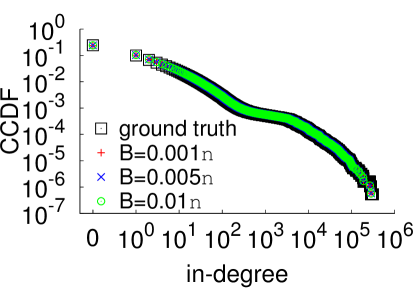
((a)) In-degree estimates

((b)) Out-degree estimates

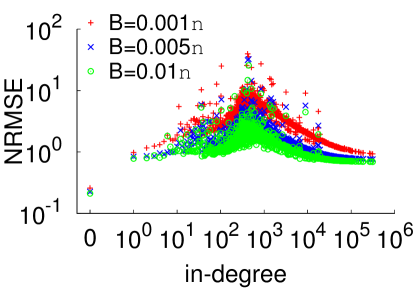
((c)) In-degree NRMSE

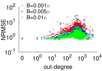
((d)) Out-degree NRMSE

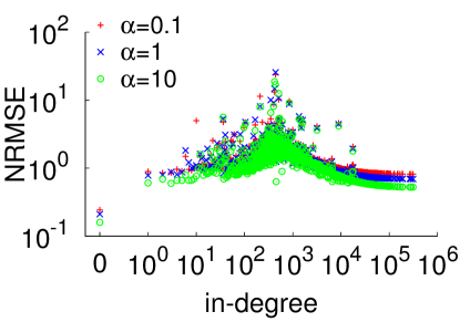
((e)) In-degree NRMSE

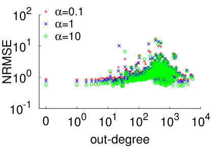
((f)) Out-degree NRMSE

Figure 12: RW^TVS^A estimates and NRMSE. (We use $\alpha=1$ in (a)-(d), and $B=0.01n$ in (e)-(f). Each result is averaged over $10,000$ runs.)

Results of method RW^TRW^A are similar to the results of RW^TVS^A, and we show them in Fig 13. First, from Figs. 13(a) and (b) we observe that RW^TRW^A can also provide well estimates of user characteristics. Second, from Figs. 13(c) and (d) we can find that when more nodes of the target graph are sampled, NRMSE decreases thereby increasing estimation accuracy. Last, from Figs 13(e) and (f) we find that when more jumps are allowed (by increasing $\alpha$ and $\beta$), NRMSE for low degree nodes decreases for both in-degree and out-degree estimates.

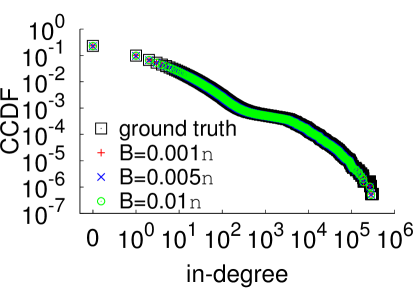
((a)) In-degree estimates

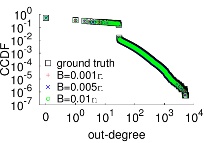
((b)) Out-degree estimates

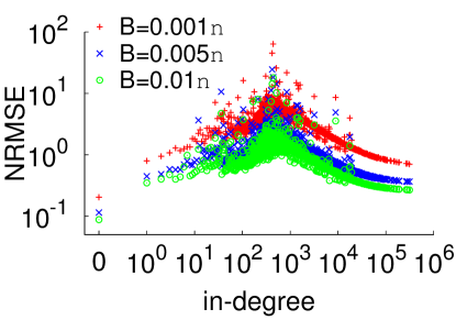
((c)) In-degree NRMSE

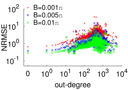
((d)) Out-degree NRMSE

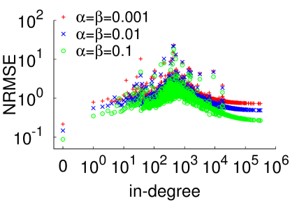
((e)) In-degree NRMSE

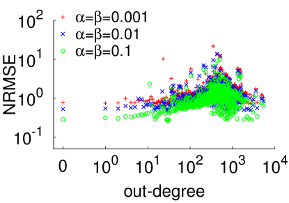
((f)) Out-degree NRMSE

Figure 13: RW^TRW^A estimates and NRMSE. (We use $\alpha=\beta=0.1$ in (a)-(d), and $B=0.01n$ in (e)-(f). Each result is averaged over $10,000$ runs.)

V Related Work

We review the related literature in this section.

Sampling methods, especially random walk based sampling methods, have been widely used to characterize complex networks. These applications include, but are not limited to, estimating peer statistics in peer-to-peer networks [14, 21], uniformly sampling users from online social networks [12, 13], characterizing structure properties of large networks [16, 15, 30, 32], and measuring statistics of point-of-interests within an area on maps [31] or venues in a region on LBSNs [18, 19]. The above literature is mostly concerned with sampling methods that seek to directly sample nodes (or samples) in target graphs (or sample spaces). However, direct sampling is not always efficient as we argued in this work.

When target graph (or sample space) can not be directly sampled or direct sampling is inefficient, several methods based on graph manipulation are proposed to improve sampling efficiency. For example, Gjoka et al. [11] use different kinds of relations (i.e., edges) to build a multigraph, which is better connected than any individual graph formed by only one kind of relations. Therefore the random walk can converge fast on this multigraph. Zhou et al. [35] exploit several criteria to rewire target graph on-the-fly so as to increase conductance and reduce mixing time of random walks. Our method differs from theirs that we do not manipulate target graphs. We study a method on how to utilize auxiliary graph and affiliation graph to assist sampling on target graph indirectly.

Birnbaum and Sirken [8] designed a survey method for estimating the number of diagnosed cases of a rare disease in a population. Directly sampling patients of a rare disease is obviously inefficient so they studied how to sample hospitals. Their method motivates us to design the VS^A method. However, as we pointed out, VS^A method cannot sample nodes that are not connected to the auxiliary graph, and we overcome this problem by designing RW^TVS^A and RW^TRW^A. Our work also complements existing sampling methods such as random walk with jumps [6, 28] and Frontier sampling [27] by removing the necessity of uniform vertex sampling on target graph.

VI Conclusion

In this work we designed three sampling methods on a hybrid social-affiliation network. The concept of hybrid social-affiliation network can help sampling a graph indirectly but efficiently. The reason of effectiveness behind our methods lies in the improvement of connectedness of target graph with the assistances of the other two graphs. We demonstrated the effectiveness of these sampling methods on both synthetic and real datasets. Our method complements existing methods in the area of graph sampling.

References

- [1] Weibo place. http://place.weibo.com, March 2014.
- [2] Weibo rate limit. http://goo.gl/WlohOj, March 2014.
- [3] Mtime. http://www.mtime.com, March 2014.
- [4] S. Aral and D. Walker. Identifying influential and susceptible members of social networks. Science, 337:337–341, 2012.
- [5] S. Asur and B. A. Huberman. Predicting the future with social media. In WI-IAT, 2010.
- [6] K. Avrachenkov, B. Ribeiro, and D. Towsley. Improving random walk estimation accuracy with uniform restarts. In the 7th Workshop on Algorithms and Models for the Web Graph, 2010.
- [7] A. L. Barabási and R. Albert. Emergence of scaling in random networks. Science, 286(5439):509–512, 1999.
- [8] Z. W. Birnbaum and M. G. Sirken. Design of sample surveys to estimate the prevalence of rare diseases: Three unbiased estimates. Vital and Health Statistics, 2(11):1–8, 1965.
- [9] J. Bollen, H. Mao, and X.-J. Zeng. Twitter mood predicts the stock market. Journal of Computational Science, 2(1):1–8, 2011.
- [10] E. Cho, S. A. Myers, and J. Leskovec. Friendship and mobility: User movement in location-based social networks. In KDD, 2011.
- [11] M. Gjoka, C. T. Butts, M. Kurant, and A. Markopoulou. Multigraph sampling of online social networks. JSAC, 29(9):1893–1905, 2011.
- [12] M. Gjoka, M. Kurant, C. T. Butts, and A. Markopoulou. Walking in Facebook: A case study of unbiased sampling of OSNs. In INFOCOM, 2010.
- [13] M. Gjoka, M. Kurant, C. T. Butts, and A. Markopoulou. Practical recommendations on crawling online social networks. JSAC, 29(9):1872–1892, 2011.
- [14] C. Gkantsidis, M. Mihail, and A. Saberi. Random walks in peer-to-peer networks: Algorithms and evaluation. Performance Evaluation, 63(3):241–263, March 2006.
- [15] S. J. Hardiman and L. Katzir. Estimating clustering coefficients and size of social networks via random walk. In WWW, 2013.
- [16] L. Katzir, E. Liberty, and O. Somekh. Estimating sizes of social networks via biased sampling. In WWW, 2011.
- [17] D. Lazer, A. Pentland, L. Adamic, S. Aral, A.-L. Barabasi, D. Brewer, N. Christakis, N. Contractor, J. Fowler, M. Gutmann, T. Jebara, G. King, M. Macy, D. Roy, and M. Van Alstyne. Computational social science. Science, 323:721–723, 2009.
- [18] Y. Li, M. Steiner, L. Wang, Z.-L. Zhang, and J. Bao. Dissecting Foursquare venue popularity via random region sampling. In CoNEXT, 2012.
- [19] Y. Li, L. Wang, M. Steiner, J. Bao, and T. Zhu. Region sampling and estimation of geosocial data with dynamic range calibration. In ICDE, 2014.
- [20] L. Lovász. Random walks on graphs: A survey. Combinatorics, Paul Erdös is Eighty, 2:353–397, 1993.
- [21] L. Massoulié, E. L. Merrer, A.-M. Kermarrec, and A. Ganesh. Peer counting and sampling in overlay networks: Random walk methods. In PODC, 2006.
- [22] S. Meyn and R. L. Tweedie. Markov Chains and Statistic Stability. Cambridge University Press, second edition, 2009.
- [23] A. Mislove, M. Marcon, K. P. Gummadi, P. Druschel, and B. Bhattacharjee. Measurement and analysis of online social networks. In IMC, 2007.
- [24] A. Mohaisen, A. Yun, and Y. Kim. Measuring the mixing time of social graphs. In IMC, 2010.
- [25] M. Mondal, B. Viswanath, P. Druschel, K. P. Gummadi, A. Clement, A. Mislove, and A. Post. Defending against large-scale crawls in online social networks. In CoNEXT, 2012.
- [26] M. E. J. Newman. The structure and function of complex networks. SIAM Review, 45(2):167–256, 2003.
- [27] B. Ribeiro and D. Towsley. Estimating and sampling graphs with multidimensional random walks. In IMC, 2010.
- [28] B. Ribeiro, P. Wang, F. Murai, and D. Towsley. Sampling directed graphs with random walks. In INFOCOM, 2012.
- [29] C. P. Robert and G. Casella. Monte Carlo Statistic Methods. Springer, second edition, 2004.
- [30] C. Seshadhri, A. Pinar, and T. G. Kolda. Triadic measures on graphs: The power of wedge sampling. In SDM’13, 2013.
- [31] P. Wang, W. He, and X. Liu. An efficient sampling method for characterizing points of interests on maps. In ICDE, 2014.
- [32] P. Wang, J. C. Lui, B. Ribeiro, D. Towsley, J. Zhao, and X. Guan. Efficiently estimating motif statistics of large networks. TKDD, 2014.
- [33] S. Wasserman and K. Faust. Social Network Analysis: Methods and Applications. Cambridge University Press, 1994.
- [34] D. J. Watts. The new science of networks. Annual Review of Sociology, 30(1):243–270, 2004.
- [35] Z. Zhou, N. Zhang, Z. Gong, and G. Das. Faster random walks by rewiring online social networks on-the-fly. In ICDE, 2013.