Selecting a Biased-Coin Design

Abstract

Biased-coin designs are used in clinical trials to allocate treatments with some randomness while maintaining approximately equal allocation. More recent rules are compared with Efron’s [Biometrika 58 (1971) 403–417] biased-coin rule and extended to allow balance over covariates. The main properties are loss of information, due to imbalance, and selection bias. Theoretical results, mostly large sample, are assembled and assessed by small-sample simulations. The properties of the rules fall into three clear categories. A Bayesian rule is shown to have appealing properties; at the cost of slight imbalance, bias is virtually eliminated for large samples.

1 Introduction

It is now over forty years since Efron (1971) introduced a biased-coin design for the partially randomized sequential allocation of one of two treatments. The intention was to provide approximate balance whenever the experiment was stopped while providing randomization to reduce biases. This was achieved by allocating the under-represented treatment with a constant probability; Efron preferred $p=2/3$. In the case of equal cumulative allocation to the two treatments, allocation was made at random. Since that time there have been many developments, recently reviewed by Biswas and Bhattacharya (2011) and compared by Zhao et al. (2012). In the comparison of these designs the emphasis has tended to be on balance. See, for example, Baldi Antognini (2008). One purpose of this review is to stress the importance of looking at both bias and balance in the assessment of designs.

Efron’s rule and its extensions are used when either there are no prognostic factors or they are ignored by the design. It is now also over thirty years since Atkinson (1982) introduced a randomized version of the sequential construction of optimum designs that can include discrete or continuous prognostic factors and can be used for a wide variety of error distributions. (A connection with Efron’s rule was a visit to Imperial College in 1981 by Rupert Miller and a discussion of Efron, 1980.) For normal homoscedastic models without covariates this randomized rule can provide a series of alternatives to Efron’s rule with controllable randomization (Smith, 1984b). Consideration of bias and loss as functions of the number of trials leads to the division of the rules, both with and without covariates, into three groups with very different properties. Balance is measured as an effective loss in the number of patients due to imbalance. Plots of loss against bias provide a cogent way to summarise the properties of designs and to determine whether designs are admissible. Efron’s original proposal is not.

The paper starts with rules without covariates. Several such rules are described in Section 2. Efron’s rule can be extended by taking values of $p$ other than $2/3$. The distribution of $D_{n}$, the difference in the number of allocations to the two treatments, forms a Markov chain, the steady-state properties of which were studied by Efron (1971). Exact distributional results for the chain are given by Markaryan and Rosenberger (2010). However, the design can become appreciably unbalanced; the rules of Soares and Wu (1983) and of Chen (1999) limit the maximum value of $D_{n}$. In addition to these rules, Baldi Antognini and Giovagnoli (2004) introduced a family of “adjustable” biased-coin rules that force balance more strongly as the difference in allocations increases. Two rather different families of rules, derived from considerations of the optimum design of experiments, are also introduced in Section 2. The rules of Smith (1984a, 1984b) are a generalization of those of Atkinson (1982) which used randomized versions of the sequential construction of optimum designs to provide allocation rules giving balance over covariates. (Consideration of rules for covariate balance starts in Section 7.) The final family of rules are derived from the Bayesian work of Ball, Smith and Verdinelli (1993) which explicitly balances inference and randomization.

The criteria for comparison of the rules, loss and selection bias, are introduced in Section 3. It is assumed that the property of interest is precise estimation of the treatment difference. Section 4 provides a survey and comparison of results for the bias and loss of the rules. Simulation is used to explore the reliability of asymptotic results.

For Efron’s biased coin, Section 4.1, the values of loss from the steady-state distribution of $D_{n}$ are compared with simulation results, showing good agreement for $p=2/3$ and $n>50$. In Section 4.2 a simple approximation is found to the steady-state distribution of $D_{n}$ for the adjustable-biased coin of Baldi Antognini and Giovagnoli (2004). This shows that the design strongly forces balance and that the loss is small. However, for odd $n$, the bias is the highest of those for the rules considered, a feature that is not obvious from the original paper. For Smith’s rule, Section 4.4, the asymptotic results are again compared with the results of simulation.

The results show very clearly the importance of assessing rules both for odd and even $n$. This point was unfortunately overlooked by Zhao et al. (2012), all of whose extensive simulation results are for even $n$. In Section 5 the averages of adjacent values of loss and bias are used in the comparison of rules. Such averages remove the effect of the parity of $n$ and confirm the general principle, for example, Atkinson (2002), that appreciably random rules have high loss and low bias, whereas rules that force balance will have low loss but high bias since forcing balance makes it easier to guess correctly which treatment will be allocated next.

The admissibility plots, introduced by Atkinson (2002), are given in Section 6 for the nine rules considered. These show the very different behaviour of the three groups of rules. In particular, Efron’s coin is inadmissible compared with an instance of the rule of Baldi Antognini and Giovagnoli (2004). The new Bayesian rule, that initially forces balance, becomes closer to random allocation as the sample size increases, thus reducing selection bias for larger samples.

These biased-coin rules can be extended to include covariates through balance over individual strata or by balance over the variables in a linear model. Section 7 introduces these approaches, together with that of randomized versions of the sequential construction of optimum designs for a linear model. The admissibility of these allocation rules is evaluated in Section 8. There is much common structure between the admissibility plots for rules with covariates in Figure 11 and those for rules without covariates in Figure 10.

The purposes of the paper include the gathering together in one place of theoretical results on the properties of the rules, which are compared to small sample results by simulation. Another purpose is to include the recent rule of Baldi Antognini and Giovagnoli (2004) in this framework and to provide some tractable theoretical results on the properties of the rule. A difference between rules without covariates and those with continuous covariates is their strong dependence on the parity of $n$. The paper closes in Section 9 with a discussion of extensions to several treatments and to models other than homoscedastic regression. We commend the Bayesian rule of Sections 4.5 and 7. In the absence of covariates the average loss for this procedure for large $n$ is equal to the loss of information on one patient, a small price to pay for the avoidance of selection bias in an asymptotically efficient rule.

2 Rules without Covariates

There are two treatments and $n$ patients of whom $N_{i}$ have received treatment $T_{i}\ (i=1,2)$. Because treatment allocation involves some randomness, the $N_{i}$ are random variables. A further important variable is the difference in the number of allocations of the two treatments $D_{n}=N_{1}-N_{2}$. The probability that patient $n+1$ is assigned to treatment 1 is given by a function $F(n_{1},n_{2})$, $N_{i}=n_{i}$ $(i=1,2).$

2.1 Efron’s Biased-Coin Design: Rule E

In Efron’s biased-coin design the allocations depend on $n_{1}$ and $n_{2}$ through the difference $D_{n}$:

$$F_{E}(x)=\cases{p,&$x<0,$\vspace*{2pt}\cr 0.5,&$x=0,$\vspace*{2pt}\cr q=1-p,&$x>0,$}$$

for $0.5\leq p\leq 1$ and $x=D_{n}$. Efron (Section 2) favours $p=2/3$, which can easily be implemented using a six-sided die. For $p=0.5$ treatment allocation becomes random, being decided by tossing a fair coin. There is no control over balance, but consistent successful guessing of the next allocation is impossible.

For $p=1$ the rule becomes that of sequential design construction and $|D_{N}|$ is either zero, when allocation is at random, or 1, when the under-represented treatment is allocated. This deterministic rule will be called Rule D and random allocation Rule R. These two rules are at the extremes of all sensible rules—theoretically the treatments could be allocated to increase imbalance, but not in a practical context. Allocation with Rule R does not depend on whether $n$ is even or odd. But, for Rule D the two values produce allocations with extreme properties, random or deterministic. The variation of properties with the parity of $n$ is a strong feature of Rule E and, particularly, of the rule in the next subsection.

2.2 The Adjustable Biased-Coin Design: Rule J

The correction toward balance in Rule E depends only on the sign of $D_{n}$ but not on its magnitude. The design may therefore sometimes become appreciably unbalanced and several rules have been suggested to reduce the variability of $D_{n}$. Part of the argument of this review is that such concerns may be overstated, given the small effect of appreciable imbalance on the statistical performance of the design for moderate $n$.

Baldi Antognini and Giovagnoli (2004) introduced a rule in which the corrective force increases with $|D_{n}|$:

$$F_{BA}(x)=\cases{\displaystyle\frac{|x|^{a}}{1+|x|^{a}},&$x<0,$\vspace*{2pt}\cr 0.5,&$x=0,$\vspace*{2pt}\cr\displaystyle\frac{1}{1+|x|^{a}},&$x>0,$}$$ (1)

for $a\geq 0$. Baldi Antognini and Giovagnoli refer to their rule as ABCD. However, all these letters have been used by Atkinson (2002). To avoid confusion, in the present paper the rule is called J for “Adjustable.”

In this rule a difference of one between treatments is treated as if it were zero and the next treatment is allocated at random. The corrective force increases with $|x|$. The value $a=0$ gives Rule R, whereas as $a\rightarrow\infty$, the rule tends to Rule D. Baldi Antognini and Giovagnoli (2004) tabulate properties for $a$ from 1 to 4.

2.3 Imbalance Tolerance

In Rule J the distribution of $D_{n}$ has support on $(-n,n)$, although, as Tables 1–3 of Baldi Antognini and Giovagnoli (2004) show, for $a$ in the range 1–4, the distribution is concentrated on a few values of $D_{n}$ near zero. Two earlier rules were formulated to restrict the range of values of $D_{n}$. In the balanced-coin design with imbalance tolerance of Chen (1999), the rule is that of Efron except that there is a reflecting barrier in the stochastic process for $D_{n}$ at $\pm b$:

$$F_{IT}(x)=\cases{1,&$x=-b,$\vspace*{2pt}\cr p,&$x<0,$\vspace*{2pt}\cr 0.5,&$x=0,$\vspace*{2pt}\cr q=1-p,&$x>0,$\vspace*{2pt}\cr 0,&$x=b.$}$$

The “big stick” design of Soares and Wu (1983) is obtained when $p=1/2$. We do not investigate the properties of these rules, which have an evolution of properties with $n$ that is similar to that of Rules E and J. These rules are related to the tractable approximation to the properties of Rule J given in Table 1.

2.4 Rule P: Permuted Block Design

Deterministic allocation, Rule D, can be thought of as allocating conceptual blocks of length 2, ensuring balance whenever $n$ is even. The blocks are “conceptual” since they are not like the blocks in a conventional experiment; they do not correspond to groups of units with common properties and they are not included in the analysis. An extension is to allocate larger randomized sequences, for example, AABABABB, ensuring balance when $n$ is a multiple of eight, but not otherwise. Efron (1971) explores some properties of designs with block sizes up to 32; Rosenberger and Lachin (2002) in their Figure 6.3 only go up to block size 10.

2.5 Smith: Rule S

Smith (1984b) investigated a family of rules in which

$$F_{S}(n_{1},n_{2})=\frac{n_{2}^{\rho}}{n_{1}^{\rho}+n_{2}^{\rho}}$$ (2)

for $\rho\geq 0.$ As $\rho\rightarrow 0$ we again obtain random allocation and, as $\rho\rightarrow\infty$, Rule D. Although the allocation probabilities depend on both $n_{1}$ and $n_{2}$, (2) can be rewritten to show that the dependence on earlier allocations is only through the ratio $D_{n}/n$. For the biased-coin rules described above, dependence is directly on the difference $D_{n}$. The results of Section 4.4 show the effect of this distinction.

The family of rules was suggested by the designs of Atkinson (1982) for randomized allocation when there are covariates over which balance is required, described in Section 7. In the absence of covariates the model contains just two parameters, the mean treatment effects $\mu_{1}$ and $\mu_{2}$. The D-optimum design maximizes the determinant of the information matrix for the two parameters, in this case minimizing the product of the variances, leading to a value of one for $\rho$. Rule A of Section 7 (the D_A-optimum design), minimizing $\operatorname{Var}(\hat{\mu}_{1}-\hat{\mu}_{2})$, is obtained when $\rho=2$.

It is simple to show that this rule, when $\rho=1,$ is the same as the adaptive biased-coin design of Wei (1978), who suggests the linear rule

$$F_{W}(n_{1},n_{2})=(1-D_{n}/n)/2.$$

Some of the results of Section 4.4 therefore also apply to Wei’s rule.

2.6 Bayesian Procedure: Rule B

Both Smith (1984b) and Markaryan and Rosenberger (2010) suggest that the rule should be designed with statistical principles in mind, such as variance of estimation and bias.

Smith (1984b) in his Section 4 derives an expression for the mean squared error of prediction when both variance and selection bias are included. His conclusion is that $\rho$ should tend to zero as $n$ becomes large. That is, for large $n$, the rule should become increasingly like random allocation. This behaviour is achieved by the Bayesian rule of this section.

In his development of methods of comparison of designs with prognostic factors, Atkinson (2002) introduces a Bayesian rule, derived from a general approach of Ball, Smith and Verdinelli (1993), which balances randomness and precision of estimation through inclusion of a parameter $\gamma$. For the allocation of one of two treatments in the absence of prognostic factors, the rule is

$$F_{B}(n_{1},n_{2})$$

(3)

$$\qquad=\frac{\{1+n_{2}/(nn_{1})\}^{1/\gamma}}{\{1+n_{2}/(nn_{1})\}^{1/\gamma}+\{1+n_{1}/(nn_{2})\}^{1/\gamma}}$$

$(0\leq\gamma\leq 1)$. As $n\rightarrow\infty$ with $\gamma=1$ random allocation, Rule R is obtained, whereas $\gamma\rightarrow 0$ gives Rule D for small $n$, that is, sequential construction of the D_A-optimum design. In this case randomization is ignored.

The important feature that distinguishes this rule from the others is its behaviour as a function of $n$. Initially, as the results in Section 6 show, when $n$ is small and $\gamma$ is also small, 0.01 in the numerical example, the rule forces balance, behaving like Rule D. However, as $n$ increases, (2.6) shows that the effect of imbalance on the allocation probability decreases. For large $n$ the rule indeed behaves increasingly like random allocation.

3 Assessing Rules: Bias and Loss

It is usual to assume that the observations are, at least approximately, normally distributed with constant variance $\sigma^{2}$ and that the treatment difference $\mu_{1}-\mu_{2}$ is the parameter of interest. The effect of imbalance due to randomization is slightly to increase the variance of the estimated difference

$$\operatorname{Var}(\hat{\mu}_{1}-\hat{\mu}_{2}) = \sigma^{2}(1/n_{1}+1/n_{2})$$

$$= n\sigma^{2}/(n_{1}n_{2}).$$

For the balanced design with $n$ even,

$$\operatorname{Var}^{*}(\hat{\mu}_{1}-\hat{\mu}_{2})=4\sigma^{2}/n\quad(n=2m),$$ (5)

where $m$ is an integer and ^∗ indicates “for the optimum design.” Of course, there will always be an imbalance of one in the optimum design when $n$ is odd ($D_{2m+1}=\pm 1$), when

$$\hskip 4.0pt\quad\operatorname{Var}^{*}(\hat{\mu}_{1}-\hat{\mu}_{2})=4\sigma^{2}/(n-1/n)\quad(n=2m+1).$$ (6)

The difference between (5) and (6) when $n=11$ is less than 1% and decreases like $n^{-2}$. The distinction in parity of $n$ will be ignored in variance comparisons.

Burman (1996) suggested rewriting (3) as

$$\operatorname{Var}(\hat{\mu}_{1}-\hat{\mu}_{2})=\frac{4\sigma^{2}}{n-L_{n}},$$

where $L_{n}$ is defined to be the “loss,” that is, the effective number of patients on whom information is lost due to the imbalance of the design. Then, from (3),

$$L_{n}=D^{2}_{n}/n$$ (7)

for even $n$. For $n$ odd we could take $L_{n}=(D^{2}_{n}-1)/n$. The value of $L_{n}$ is random, depending on the outcome of the particular randomization. The expected value of $L_{n}$ is written

$${\mathcal{L}}_{n}=(\operatorname{Var}D_{n})/n,$$ (8)

since, for the designs considered here, E$D_{n}=0$.

An important related statistical quantity is the efficiency of the design,

$$E_{n}=\frac{\operatorname{Var}^{*}(\hat{\mu}_{1}-\hat{\mu}_{2})}{\operatorname{Var}(\hat{\mu}_{1}-\hat{\mu}_{2})}=\frac{n-L_{n}}{n}=1-L_{n}/n.$$ (9)

These quantities are highly informative about the properties of all designs considered.

The loss $L_{n}$ depends on the particular sequence of randomized allocations. Interest here is in the expectation E$L_{n}={\mathcal{L}}_{n}$, approximated by $\bar{L}_{n}$, the average over $n_{\mathrm{sim}}$ simulations. For Rule S the expected value of the loss ${\mathcal{L}}_{n}$ has a constant limit as $n\rightarrow\infty$ (Section 4.4). For random allocation, a result that goes back at least to Cox (1951) is that ${\mathcal{L}}_{\infty}=1.$ For the biased-coin Rules E and J, $\operatorname{Var}D_{n}$ approaches from below a finite limit as $n\rightarrow\infty$. The loss therefore decreases with $n$. Simulation results on the distribution of $L_{n}$ for rules with covariates are presented by Atkinson (2003).

Statistical power is extremely important in the practical assessment of designs for clinical trials. Plots like those in Figure 3.1 of Rosenberger and Lachin (2002), and the similar plot in Pocock (1983), show how very large the value of $D_{n}$ has to be to cause a measurable effect on power. For both forms of behaviour of loss with increasing $n$, it follows from (9) that the efficiency of the design goes to one as $n\rightarrow\infty$. Except for very small trials, the average effect of imbalance on (3) will be negligible. For a particular randomization, the interpretation of $L_{n}$ as a number of patients on whom information is lost leads directly to the calculation of loss in power due to the imbalance from randomization.

Randomization and balance are in conflict. A numerical measure for randomization is selection bias (Blackwell and Hodges, 1957) which measures the ability to guess the next treatment to be allocated. Bias depends on the design, the guessing strategy and, for some rules, the value of $n$. For a particular combination of strategy and design the expected bias ${\mathcal{B}}_{n}$ is estimated from $n_{\mathrm{sim}}$ simulations as

$$\bar{B}_{n} = (\mbox{number of correct guesses}$$

$$\hskip 4.0pt\mbox{of allocation to patient }n$$

$${}-\mbox{number of incorrect guesses})/n_{\mathrm{sim}}.$$

This definition is similar to that of (4.2) of Smith (1984b). The guessing strategy used in the numerical comparisons of the next sections is the sensible one of guessing that the treatment for which the allocation probability $p\geq 0.5$ will be selected.

Atkinson (2002) calculated $\bar{B}_{n}$ from the binary variables in (3). It is, however, more efficient, as is done here, to follow Heritier, Gebski and Pillai (2005) and average the expectations $2p-1$.

The customary justifications for randomization in experiments include the avoidance of bias. Amongst many others, Efron (1971) and Smith (1984b) consider that selection bias should not be an issue in double-blind trials with treatment allocation made remotely from the trial, although it may be if there are local attempts toward institutional balance (Lagakos and Pocock, 1984). However, a trial without randomization appears to lack objectivity. Accordingly, they study the effect of biased-coin designs on freedom from accidental bias due to omitted factors, including time trends and, in the case of Smith (1984b), correlated errors and outliers. The conclusion of Smith (1984b) is that biased-coin designs that are not as random as Rule R provide good protection against several sources of bias and that selection bias is a good measure of the properties of the design.

There are several related measures of selection bias. For example, Efron (1971) and Markaryan and Rosenberger (2010) use excess selection bias, that is, the expected number of correct guesses in excess of those expected when allocation is at random. A slight advantage of ${\mathcal{B}}_{n}$ is that the values lie between 0 and 1. However, one measure is a linear function of the other, so that the ranking of rules is not changed by the choice of measure.

Smith (1984b) in his equation 4.2 defined the selection bias ${\mathcal{B}}_{n}$, but found the average bias over all allocations up to $n$. Average bias was also used by Baldi Antognini and Giovagnoli (2004) and by Zhao et al. (2012), who, however, calculate the mean number of correct guesses. In the present paper the measure used is $\bar{B}_{n}$, which refers solely to guesses of the $n$th allocation. An advantage of this measure is that it reveals whether there is a strong dependence of the bias on the parity of $n$. A book length discussion of forms of selection bias is due to Berger (2005). Proschan, Brittain and Kammerman (2012) briefly discuss some situations in which blinding is impossible and selection bias may seriously distort inferences.

4 Analytical and Numerical Results on Bias and Loss

Analytical results for bias and loss are available for some rules. They are summarized by allocation rule in the following section. For Rules E and J the distribution of the values of $D_{n}$ forms a Markov chain. The analytical results come from the steady-state distribution of $D_{n}$. The value of ${\mathcal{B}}_{n}$ depends on the distribution of $D_{n-1}$, whereas that of ${\mathcal{L}}_{n}$ requires the distribution of $D_{n}$. For Rule S the results are asymptotic and do not depend on the parity of $n$. Simulation is used to check the properties of the rules for finite $n$ and to show some properties of Rule B.

There are also related results on the distribution of the number of patients $N_{i}$ allocated to each treatment. For Rules E and J the limiting Markov chain for the distribution of $D_{n}$ leads to the result that $n^{-1/2}D_{n}$ goes to 0 in probability, so that $N_{i}$ goes to one half. For Rule S the proportions have an asymptotically normal distribution depending on the value of $\rho$ in (2). The details are in Section 4.4.

Figure 1: Efron’s coin with $p=2/3$—Rule E$(2/3)$. Left-hand panel, average loss $\bar{L}_{n}$, right-hand panel, average bias $\bar{B}_{n}$. 100,000 simulations.

4.1 Efron’s Biased Coin: Rule E

If $D_{n-1}=0$, allocation to patient $n$ is at random and the bias is zero. For all other values the bias, conditional on the value of $D_{n-1}$, is $2p-1$. The steady-state probabilities that $D_{n}=0$ are given by Efron (1971) and by Markaryan and Rosenberger (2010) who both write $r=p/q=p/(1-p).$ Then, for integer $m$,

$$\mathop{\lim}_{n\rightarrow\infty}P(D_{2m}=0)=\frac{r-1}{r}=\frac{2p-1}{p},$$

(11)

$$\eqntext{\mbox{with }P(D_{2m-1}=0)=0.}$$ (12)

When $n$ is even, that is, $n=2m$, it follows from (4.1) that

$${\mathcal{B}}_{2m}=2p-1.$$

When $n$ is odd, $P(D_{2m}\neq 0)=(1-p)/p$ and

$${\mathcal{B}}_{2m-1}=(2p-1)(1-p)/p.$$

For the original coin with $p=2/3$,

$$\quad{\mathcal{B}}_{2m}(2/3)=1/3\quad\mbox{and}\quad{\mathcal{B}}_{2m-1}(2/3)=1/6.$$ (13)

The right-hand panel of Figure 1 shows average simulated values $\bar{B}_{n}$ for Rule E($2/3$), that is, Efron’s coin. Although the two values in (13) are calculated from the steady-state distribution of $D_{n}$, the figure shows that the bias immediately settles down to oscillate between these two values.

For random allocation $p=0.5$ and ${\mathcal{B}}_{n}(0.5)=0$, whether $n$ is odd or even. As $p$ increases, ${\mathcal{B}}_{2m}\rightarrow 1$, whereas ${\mathcal{B}}_{2m-1}$ has a maximum at the famous number $(\sqrt{5}-1)/2=0.6180$ before declining to zero.

Equation (8) shows that the loss ${\mathcal{L}}_{n}=(\operatorname{Var}D_{n})/n$. Expressions for $\operatorname{Var}D_{n}$ from the steady-state distribution are given by Markaryan and Rosenberger (2010), from which expressions for ${\mathcal{L}}_{n}$ follow.

These values of ${\mathcal{L}}_{n}$ again depend on whether $n$ is even or odd:

$${\mathcal{L}}_{2m} = \frac{4r(r^{2}+1)}{n(r^{2}-1)^{2}},$$ (14)

$${\mathcal{L}}_{2m-1} = \biggl{\{}\frac{8r^{2}}{(r^{2}-1)^{2}}+1\biggr{\}}\Big{/}n.$$ (15)

Re-expressions as functions of $p$ do not provide any insight.

The left-hand panel of Figure 1 shows the average values of loss, $\bar{L}_{n}$, for $p=2/3$. Unlike the plot of bias in the right-hand panel, this plot shows only a small effect of the parity of $n$. As is to be expected, the loss is larger for odd $n$. Since the rule becomes random allocations as $p$ approaches 0.5 and sequential balancing, Rule D, as $p$ approaches one, it is to be expected that the ratio of loss for odd to even $n$ increases with $p$: for $p=0.55$ the ratio is 1.0002; for Efron’s coin with $p=2/3$ it has only risen slightly to 1.0250, becoming 1.1333 when $p=0.75$.

Perhaps of greater importance is the approach of the loss to the value in (8) when the steady-state variance is used. Table 2 of Markaryan and Rosenberger (2010) gives exact values of the variance of $D_{n}$ for $n$ both even and odd for a range of values of $p$. Convergence to the asymptotic value is faster for larger values of $p$. For small $n$ and $p$ near 0.5 the exact variance is appreciably smaller than that at the steady-state.

To illustrate the effect on loss, let the steady-state variance be denoted $\operatorname{Var}D_{\infty}$. Then the loss should decrease as $1/n$ and the ratio $n\bar{L}_{n}/D_{\infty}$ should tend toward one. Figure 2 illustrates this for three values of $p$. For $p=0.55$ the ratio has only reached 0.85 when $n=200$. However, for $p=2/3$, values around one are reached around $n=50$. For $p=3/4$ the values are above 0.9 for $n\geq 8$. The steady-state values of loss given in (7) and (15) provide useful guidance for all coins except those with very low values of $p$, which are unlikely to be used in practice, or with small values of $n$.

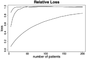
Figure 2: Rule E($2/3$). Convergence of ${\mathcal{L}}_{n}$ to the steady-state value given by (7) or (8): ratio $n\bar{L}_{n}/D_{\infty}$. Reading down, $p=3/4$, $2/3$ and 0.55. 100,000 simulations.

These results about bias and loss indicate that the properties of Efron’s biased-coin are well understood, both asymptotically and for smaller samples. In theory, exact results for ${\mathcal{L}}_{n}$ can be obtained from the analytical expressions for the distribution of $D_{n}$ given in Markaryan and Rosenberger (2010). However, the authors warn in their Section 3 that care is needed in the numerical calculation of the summations they present, since these involve factorials of large numbers and powers of numbers less than one. As here, simulation may sometimes be an easier way to obtain an idea of the properties of a rule for a variety of parameter values.

Figure 3: Adjustable biased-coin with $a=3$—Rule J(3). Left-hand panel, average loss $\bar{L}_{n}$, right-hand panel, average bias $\bar{B}_{n}$. 100,000 simulations.

4.2 The Adjustable Biased-Coin: Rule J

Figure 3 shows the average values of loss $\bar{L}_{n}$ and bias $\bar{B}_{n}$ for Rule J with parameter $a=3$. These plots are similar in structure to those for Rule E in Figure 1, although the values of loss are lower for Rule J and show a greater effect of the parity of $n$. The surprise, however, is the more extreme values of bias, which are not to be expected from the presentation of Baldi Antognini and Giovagnoli (2004).

There are some theoretical results for the balance, bias and power of Rule J. Baldi Antognini and Giovagnoli (2004) provide asymptotic comparisons of selection bias with Rule E and show that their rule has smaller bias than E($2/3$) for any value of $a$. The power comparisons of Baldi Antognini (2008) are for a more general family of rules than J. One result (Corollary 3) is that for any sample size a rule with $F(-1)\geq p$ is uniformly more powerful that $E(p)$. The rule studied here, (1), does not meet this condition. The rate of decrease of the loss associated with Rule J is shown by Baldi Antognini and Zagoraiou (2011) to be $1/n$.

The adjustable biased-coin (1) combines avoidance of excessive imbalance with greater randomness than Efron’s rule in the centre of the distribution of $D_{n}$. For $D_{n}=-1,0$ or 1 the probability of moving to $D_{n+1}=D_{n}+1$ or $D_{n}-1$ is 0.5; values of $D_{n}=\pm 2$ are therefore frequent. However, except for small $a$, absolute values greater than or equal to four rarely occur—see the numerical calculations in Tables 1–3 of Baldi Antognini and Giovagnoli (2004). We therefore use as an approximation a truncated Markov chain for $D_{n}$. For example, for $a=2$, the equilibrium probability that $|D_{n}|\geq 4$ is less than 0.013 for $n$ even and less than 0.001 for $n$ odd. To obtain a tractable approximation to the equilibrium probabilities of this rule, and so to calculate approximate values of the bias and loss, we examine the approximation of the rule by the truncated Markov chain on the values $-3$ to 3. This truncated rule is a hybrid between those of Soares and Wu (1983) and of Chen (1999) introduced in Section 2.3.

Table 1: Stationary distribution of the approximation to Rule J; $p=2^{a}/(1+2^{a})$

$\bolds{D_{n}}$	$\bolds{-3}$	$\bolds{-2}$	$\bolds{-1}$	$\bolds{0}$	$\bolds{1}$	$\bolds{2}$	$\bolds{3}$
$n$ odd	$\frac{1-p}{2(1+p)}$	0	$\frac{p}{1+p}$	0	$\frac{p}{1+p}$	0	$\frac{1-p}{2(1+p)}$
$n$ even	0	$\frac{1}{2(1+p)}$	0	$\frac{p}{1+p}$	0	$\frac{1}{2(1+p)}$	0

The stationary distribution of $D_{n}$ for this approximation is displayed in Table 1 where $p=2^{a}/(1+2^{a})$. Given the stationary distribution, it is straightforward to calculate the loss and bias. The loss for a difference of $D_{n}$ is $D^{2}_{n}/n$. The biases for the central values of $D_{n}$, that is, 0 and $\pm 1$, are zero, since the allocation is at random. For $|D_{n}|=2$ there is a probability of $p$ of allocating the underrepresented treatment and the conditional bias is $2p-1$. For $|D_{n}|=3$ the underrepresented treatment is always allocated and the bias is one. Taking expectations over the stationary distributions for odd and even $n$ leads to

$$n\mbox{ even:}\quad{\mathcal{L}}_{n}=\frac{9-7p}{n(1+p)},\quad{\mathcal{B}}_{n}=\frac{2p-1}{1+p},$$

(16)

$$n\mbox{ odd:}\quad{\mathcal{L}}_{n}=\frac{4}{n(1+p)},\quad{\mathcal{B}}_{n}=\frac{1-p}{1+p}.$$

As for Rule E, for this approximation the expected loss decreases with $n$, but the bias is independent of $n$, in line with the plots of Figure 3.

Table 2: Rule J. Approximate values of ${\mathcal{L}}_{n}$ and ${\mathcal{B}}_{n}$ ($n=199$ and 200) from the approximation (4.2). Bracketed values below are averages $\bar{B}_{n}$ and $\bar{L}_{n}$ from 100,000 simulations

$\bolds{a}$	$\bolds{L_{199}}$	$\bolds{L_{200}}$	$\bolds{B_{199}}$	$\bolds{B_{200}}$
1	0.0131	0.0120	0.2000	0.2000
	(0.0172)	(0.0177)	(0.2369)	(0.1382)
2	0.0095	0.0111	0.3333	0.1006
	(0.0100)	(0.0120)	(0.3408)	(0.1006)
3	0.0074	0.0106	0.4118	0.0588
	(0.0075)	(0.0107)	(0.4152)	(0.0579)
4	0.0062	0.0103	0.4545	0.0303
	(0.0062)	(0.0103)	(0.4545)	(0.0303)

Figure 4: Permuted block design, block size eight—Rule P. Left-hand panel, loss ${\mathcal{L}}_{n}$, right-hand panel, bias ${\mathcal{B}}_{n}$; the value of $-1$ comes from incorrect guessing.

Table 2 gives a comparison of the values of ${\mathcal{L}}_{n}$ and ${\mathcal{B}}_{n}$ from the approximation (4.2) with, in brackets, the average values from 100,000 simulations for $n=199$ and 200. The table shows how good the approximation is, both for bias and loss, when $a$ is as small as 2, that is, $p=4/5$. For this and higher values of $a$, the value of $p$ is sufficiently large that the distribution of $D_{n}$ is indeed concentrated in the range $-3$ to 3. Better approximations for both small $a$ and small $n$ can be found by putting the reflecting barriers of the Markov process further out than $\pm 3$.

There are three substantive points in these results. The first is the extremely small values of loss, even when $a=1$. For these values of $n$ an arbitrarily stopped trial will be very close to balance. The second is that, although the values of loss depend on the parity of $n$, the values are so small that the inferential effect is negligible. The third is the extremely high value of bias when $n$ is even. As $p\rightarrow 1$ the approximations in (4.2) show that the bias tends to 0.5 for $n$ even, whilst going to zero for $n$ odd. This behaviour raises the question of how to compare rules which have such different properties for odd and even $n$.

4.3 Rule P: Permuted Block Design

As an example of a permuted block design let $n=8$. A typical design allocates treatments in the order AABABABB. The underrepresented treatment is guessed with random guessing for the first allocation. Then ${\mathcal{B}}_{1}=0$. Thereafter, ${\mathcal{B}}_{n}$ will be one when the underrepresented treatment is allocated and $-1$ when the overrepresented treatment is allocated. If the length of the block is known, the last guess will always be correct, as balance is attained. For example, guessing the underrepresented treatment in AABABABB gives ${\mathcal{B}}_{2}=-1$ and ${\mathcal{B}}_{8}=1$.

Figure 5: Smith’s rule with $\rho=5$—Rule S(5). Left-hand panel, average loss $\bar{L}_{n}$, right-hand panel, average bias $\bar{B}_{n}$. 100,000 simulations.

Figure 4 shows loss and bias for the rule with block size 8. Loss quickly decreases with $n$; since there is balance when each block is completed, ${\mathcal{L}}_{8m}=0$. Because the allocation is deterministic, the fine detail of the plot shows repetition of the same eight-allocation pattern of loss, decreasing as $1/n$. The right-hand panel shows bias up to $n=16$, that is, two cycles of guessing in ignorance of the structure.

Figure 1 of Efron (1971) compares a measure of selection bias for several biased-coin Rules E with permuted blocks of size $2m$. For $m=9$ the bias is similar to that of E($2/3$). As $m$ increases, the rule becomes more like random allocation, that is, Rule E with $p\rightarrow 0.5$. Figure 6.3 of Rosenberger and Lachin (2002) compares bias over $n$ for values of $m$ from 1 (deterministic allocation) to 5. These comparisons are over all possible permutations of the $2m$ allocations, rather than for a specific permutation, like that of Figure 4 that would be used in a particular trial. Bailey and Nelson (2003) advocate restricted randomization, in which permutations with an “obvious” pattern are not considered. Those that become too unbalanced could also be excluded.

The ability to guess correctly depends on what is known about the structure of the design. If it were known that this structure of eight treatments were to be repeated, then ${\mathcal{B}}_{n}$ would be one for all $n>8$. Randomly relabeling treatments A and B, using several permutations or changing the block size are all ways in which the value of ${\mathcal{B}}_{n}$ could be kept small, although at some administrative cost.

4.4 Smith’s Rule: Rule S

Figure 5 shows the values of average loss and average bias for 100,000 simulations of Smith’s rule with $\rho=5$. Apart from the few initial values of $n$, the values of loss in the left-hand panel are virtually constant, whereas the average bias decreases with $n$. As it does so, the effect of the parity of $n$ disappears. This is very different behaviour from that for the two-biased coin Rules J and E in which bias is constant with $n$, although depending on parity, whilst loss decreases as $1/n$.

The properties of the biased-coin designs in the earlier sections were found from the Markov chain formed by the values of $D_{n}$. This structure is not available for Rule S and asymptotic arguments are used instead. From equation (4.1) of Smith (1984b),

$${\mathcal{L}}_{n}=1/(1+2\rho).$$ (17)

The asymptotic distribution of ${L}_{n}$ follows from Smith (1984a) who shows the convergence in distribution of $n^{-1/2}D_{n}\rightarrow{\mathcal{N}}\{0,1/(1+2\rho)\}$. From (8) the asymptotic distribution of loss is therefore

$$L_{n}\sim X_{1}^{2}/(1+2\rho),$$

where $X_{1}^{2}\sim\chi^{2}_{1}$.

The asymptotic distribution of $D_{n}$ also provides the asymptotic distribution of $N_{i}$, the number of patients receiving treatment $i$. Since $\operatorname{Var}(N_{i})=\operatorname{Var}(D_{n})/4$, asymptotically,

$$n^{-1/2}N_{i}\sim{\mathcal{N}}\bigl{[}1/2,1/\bigl{\{}4(1+2\rho)\bigr{\}}\bigr{]}.$$ (18)

For random allocation ($\rho=0$) the variance is $1/4$.

In his (4.3) Smith further uses the asymptotic normality of $D_{n}$ to show that, as $n\rightarrow\infty$,

$${\mathcal{B}}_{n}\cong\rho\sqrt{2/\bigl{\{}n\pi(1+2\rho)\bigr{\}}}.$$ (19)

Figure 6: Rule S(5). Approach of loss and bias to asymptotic values. Left-hand panel, ratio of $\bar{L}_{n}$ to ${\mathcal{L}}_{n}$ (17). Right-hand panel, ratio of $\bar{B}_{n}$ to ${\mathcal{B}}_{n}$ (19). 100,000 simulations.

Figure 6 explores the relationship between the average values of loss and bias plotted in Figure 5 and the asymptotic values given above. The left-hand panel shows the ratio of the two estimates of expected loss, $\bar{L}_{n}$ and ${\mathcal{L}}_{n}$. Initially there is a slight effect of the parity of $n$ on the ratio, but, from $n=15$, the ratio decreases from less than 1.2 toward one as $n$ increases. The plot of the ratio for bias, $\bar{B}_{n}/{\mathcal{B}}_{n}$ in the right-hand panel, shows the much stronger effect of odd and even $n$ which was also apparent in Figure 5, but is ignored in the asymptotic expression (19). The ratio is centered on one with the effect of parity steadily decreasing.

The indication of Figure 5 is that the asymptotic results for Rule S provide a good guide to the behaviour of this rule, even for small values of $n$.

4.5 Bayes: Rule B

Unlike the other rules of this section, there are no theoretical results for the loss and bias of Rule B, except that it moves from deterministic allocation, Rule D, to random allocation as $n$ increases. The rate of transition from one form of allocation to the other depends on the value of the parameter $\gamma$.

Figure 7: Bayes rule with $\gamma=0.01$—Rule B(0.01). Left-hand panel, average loss $\bar{L}_{n}$, right-hand panel, average bias $\bar{B}_{n}$. 100,000 simulations.

The final plot of bias and loss for a single rule without covariates is in Figure 7 for the Bayes rule with $\gamma=0.01$. These plots are unlike any we have so far seen. The left-hand panel shows that the loss starts close to zero and then gradually increases with $n$. Initially, the balancing effect of the design is such that the loss depends on the parity of $n$. The bias, in the right-hand panel, starts by alternating between zero and one, as it does for deterministic allocation. As $n$ increases the bias decreases, as the rule becomes increasingly like random allocation.

5 Adjacent Averages

A striking feature of Figures 1 and 3 is the strong dependence of the bias on whether $n$ is even or odd, although this is not a feature of all rules. In the next section we compare several of the rules of Section 4 for various parameter values. Table 3 extends the simulation results of Table 2 to these nine rules.

Table 3: Average values of loss, $\bar{L}_{n}$, and bias, $\bar{B}_{n}$ ($n=199$ and 200), and adjacent averages of these values, $\tilde{L}_{200}$ and $\tilde{B}_{200}$, for nine rules arranged according to adjacent average bias. 100,000 simulations

Rule	$\bolds{\bar{L}_{199}}$	$\bolds{\bar{L}_{200}}$	$\bolds{\bar{B}_{199}}$	$\bolds{\bar{B}_{200}}$	$\bolds{\tilde{L}_{200}}$	$\bolds{\tilde{B}_{200}}$
D	0.0050	0.0000	0.0022	1.0000	0.0025	0.5011
E($2/3$)	0.0228	0.0221	0.1707	0.3371	0.0224	0.2549
J(3)	0.0075	0.0107	0.4152	0.0579	0.0091	0.2366
E(0.55)	0.2139	0.2127	0.0848	0.1041	0.2133	0.0944
S(5)	0.0916	0.0916	0.0861	0.0874	0.0916	0.0868
S(2)	0.2001	0.2002	0.0491	0.0518	0.2002	0.0505
B(0.01)	0.2764	0.2773	0.0279	0.0313	0.2769	0.0296
B(0.1)	0.6972	0.6982	0.0050	0.0032	0.6917	0.0041
R	1.0010	1.0007	0.0022	0.0025	1.0008	0.0024

In the table the rules are arranged in order of decreasing bias. The first four columns are the average losses and biases from 100,000 simulations when $n=199$ and 200. As the figures for individual rules have shown, the values of bias are more sensitive to the parity of $n$ than are the values of loss. The strongest difference in bias between $n$ odd and $n$ even is for deterministic allocation, Rule D, when the theoretical value of the bias is one or zero depending on whether $n$ is even or odd.

We have already seen in Section 2.1 that the expected values of bias for Efron’s rule, E($2/3$), are $1/6$ and $1/3$. For the adjustable biased-coin J(3), the results of Table 2 are that the two values of bias are 0.4118 and 0.0588. As $p$ decreases toward 0.5 in Efron’s rule, the allocation becomes more random and the difference in properties for odd and even $n$ decreases. When $p=0.55$ the expected value of bias for $n=199$ and 200 are 0.0818 and 0.1. The remaining rules in the table all have values of bias less than 0.1.

Trials are equally likely to stop with $n$ odd or even. Therefore, in order to compare rules, we use adjacent averages and write

$$\tilde{L}_{n}=(\bar{L}_{n-1}+\bar{L}_{n})/2,$$ (20)

with a similar definition for $\tilde{B}_{n}.$ These averages remove the effect of oscillation between the two values, particularly of bias, and allow an insightful comparison of rules.

For the rules with continuous covariates compared in Section 8 the maximum value of ${\mathcal{B}}_{n}$ is one. But, without covariates, the most extreme adjacent values of bias are zero and one, so that, with adjacent averaging, the maximum value of E$\tilde{B}_{n}$ is 0.5. The rules in Table 3 are arranged in decreasing order of $\tilde{B}_{200}$. The largest theoretical value is 0.5 for Rule D. The only other rules with appreciable averages for adjacent bias are E($2/3$) and J(3) with values around 0.25; for all other rules the values are less than 0.1.

It is a general principle in the comparison of these rules that acceptable rules with high bias have low loss and conversely. Atkinson (2002) provides examples for allocation rules with covariates. And, indeed, in Table 3 the values of $\tilde{L}_{200}$ increase from a theoretical value of 0 for Rule D to 1 for Rule R. The only exceptions are the two Efron rules; E($2/3$) has higher loss and higher bias, at $n=200$, than J(3). Similarly, E(0.55) has higher loss and bias than either of the Rules S. These results, however, only provide a snapshot of the behaviour of the rules at $n=200$. We now look at plots of the adjacent averages of bias and loss over a range of values of $n$.

Figure 8: Simulated values of adjacent averages of loss and smoothed bias for five rules. Left-hand panel, $\tilde{L}_{n}$. Reading down: R, random allocation; E(0.55), Efron’s rule with $p=0.55$; E($2/3$); adjustable biased-coin J(3) and D, deterministic allocation. Right-hand panel, $\tilde{B}_{n}$. Same notation, reading up. 100,000 simulations.

Figure 8 shows plots of adjacent averages of bias and loss for the rules in which loss decreases as $1/n$ and the bias is constant, that is, Rules J and E. Also included are random and deterministic allocation, which are the special cases of Rule E as $p\rightarrow 0.5$ and one. The values of $\tilde{L}_{n}$ in the left-hand panel form a series of values of loss decreasing steadily with $n$. Likewise, the right-hand panel shows a series of virtually constant values for $\tilde{L}_{n}$. The only surprise is that Rule J(3) has lower loss and lower bias than E($2/3$). The argument of the next section is that Rule E($2/3$) is therefore inadmissible. Otherwise, the order of the rules is reversed between the panels for loss and bias.

Figure 9: Simulated values of adjacent averages of loss and smoothed bias for four rules. Left-hand panel, $\tilde{L}_{n}$. Reading down: B, Bayes rule with $\gamma=0.1$; B, Bayes rule with $\gamma=0.01$; S, Smith’s rule with $\rho=2$ and Smith’s rule with $\rho=5$. Right-hand panel, $\tilde{B}_{n}$. Same notation, reading up. 100,000 simulations.

The plots of $\tilde{L}_{n}$ for Rule S in the left-hand panel of Figure 9 are virtually constant, whereas those for Rule B increase with $n$. As $n$ increases, Rule B$(0.1)$ becomes increasingly like random allocation at a faster rate than does the rule with $\gamma=0.01$. The plots for $\tilde{B}_{n}$ in the right-hand panel are in the reverse order by the time $n$ is around 100; as the loss for Rule B increases, the bias decreases faster than $1/n$ as allocation becomes increasingly random.

6 Admissibility

A good rule should have low loss and low bias for all $n$. In order to compare loss and bias, Atkinson (2002) suggested plotting loss against bias as a function of $n$, thus combining in one plot the two panels of plots like Figure 9. The shape that this curve takes will depend upon the individual rule; from the curves in Figures 8 and 9 it is clear that there will be three general forms of trajectory. A good rule will be in the lower left-hand corner of the plot. But usually, for any particular $n$, a rule with lower loss than another will have higher bias. A rule for which both values are higher is said to be inadmissible.

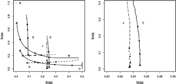
Figure 10: Admissibility. Simulated values of adjacent averages of loss and smoothed bias for nine rules. Left-hand panel, vertical continuous lines from the left—E(0.55) and E($2/3$); vertical dotted and dashed line—J(3); horizontal dashed lines reading down—S(2) and S(5); continuous lines, reading down—B(0.1) and B(0.01). Symbols: $\blacksquare\ n=15;\bullet\ n=25$; $\circ\ n=50$; $\Delta\ n=200.$ Right-hand panel, J(3) and E($2/3$). 100,000 simulations.

The left-hand panel of Figure 10 is the admissibility plot for the nine rules considered in this paper. Rules R and D plot virtually as points at $(0,1)$ and $(0.5,0)$, respectively. Both are admissible since 0 is the minimum possible value of bias or loss. The other rules in Figure 8, which have constant bias, plot as vertical lines. The symbols on the lines correspond to values of $n$ with $\Delta$ denoting $n=200$. For E(0.55) the bias is around 0.09 while the loss decreases steadily with $n$. For Rules J(3) and E($2/3$) the bias is higher but the loss is lower for specific $n$. Rule E(0.55) is therefore admissible when compared with these two rules. However, the comparison of Rules J(3) and E($2/3$) in the right-hand panel of the figure shows that E($2/3$) is not admissible. For any $n$ over the range 10 to 200 it is possible to achieve lower loss and bias by using Rule J(3).

The Rules S in Figure 9 have virtually constant loss and so plot as almost horizontal lines; S(5) plots below S(2) as it has lower loss, but it lies to the right of the curve for S(2) for any particular $n$. As $n$ increases the bias decreases and the curves tend toward the left-hand axis. The curves for Rule B form a third family. These start close to Rule D, but the bias decreases as the loss increases. For $n=10$ they have the smallest loss for all rules except D and, for $n=200$ the lowest bias for all rules except R. For smaller values of $\gamma$ than these, the emphasis in Rule B is increasingly on balancing the design and a series of curves is obtained which lie below those plotted. However, for any $n$, the points are to the right of those for larger $\gamma$ so that all these rules are admissible.

The right-hand panel of Figure 10 shows that E($2/3$) is not admissible compared to J(3) over all values of $n$ considered. The comparison of results in Table 3 indicated that, for $n=200$, Rule E(0.55) had higher bias and loss than Rules S. But the left-hand panel of the figure shows that, for $n$ less than 50, the bias of S(2) is greater than that of E(0.55). Further, the indication is that, for $n$ slightly greater than 200, E(0.55) has lower loss than S(5). In addition, for almost all $n$ in the figure, S(2) has higher bias than E(0.55). Neither rule dominates the other over all considered values of $n$.

Superficially, Figure 10 appears similar to several of the figures in Zhao et al. (2012) where a measure of bias is plotted against maximum absolute imbalance, that is, the maximum of $|D_{n}|$ in each simulation. However, the plots are for fixed even $n$ for a series of parameter values. Information on the dependence on $n$ is not clear. As Figure 3 for Rule J shows, very different conclusions can be reached about the properties of a rule if only odd or even values of $n$ are considered. Section 3 emphasizes the statistical basis of the criteria, selection bias and loss, used here. Use of the maximum of $|D_{n}|$ favours rules in which the values of $D_{n}$ are bounded and, indeed, the rule of Soares and Wu (1983), which is random over a restricted range, performs best in the comparisons of Zhao et al. (2012); the rule of Baldi Antognini and Giovagnoli (2004) is not included in their comparisons.

7 Designs with Covariates

When measurements of some covariates are available before treatment allocation, the randomization of patients should allow for the covariates. Rosenberger and Sverdlov (2008) present a survey of the approaches of statisticians and clinical trialists to the handling of covariates in the design of clinical trials. Their numerical examples are for binomial responses, which are naturally heteroscedastic. They stress, and illustrate by example, that under such conditions, balance over covariates does not lead to the most efficient designs. In contrast, the next sections of this paper continue the study of rules for normal responses with constant variance. Under these conditions balance of covariates over treatments reduces dependence on the correctness of the assumed form of the relationship between response and covariates. Even if the covariates are to be adjusted for in the analysis, balance ensures estimates of effects with lower variance (Baldi Antognini and Zagoraiou, 2011). Comments on designs for heteroscedastic models and generalized linear models are given briefly in Section 9.

Comparisons of the loss, bias and admissibility of several rules with covariates and normally distributed errors are given by Atkinson (2002) and in Chapter 6 of Atkinson and Biswas (2014). However, these comparisons do not include Rule J. Accordingly, the focus here is on extensions of this rule to include covariates.

Rule M: Minimization—Pocock and Simon. We start with two deterministic rules which do not model the dependence of the response on the covariates. The minimization rule of Pocock and Simon (1975) depends on calculating the total effect on all measures of marginal imbalance when treatment $j^{+}$ is allocated. If there are $m$ covariates $x$, there will be $m$ measures to be summed. The individual measures count the number of observations in each category of the covariate. Continuous covariates therefore have to be categorized.

Let the total effect on imbalance be $C(j^{+})$. The allocations are ranked so that

$$C\bigl{(}[1]\bigr{)}\leq C\bigl{(}[2]\bigr{)}.$$

In this deterministic allocation treatment [1] is allocated, with random allocation if both treatments have the same value of $C(j^{+})$.

The calculations are exemplified by Senn, Anisimov and Fedorov (2010) and Atkinson (2002) as well as by Pocock and Simon (1975). In the simulations of Section 8 standard normal covariates are dichotomized at 0.

Rule C: Balanced covariates. There are $m$ covariates, either discrete or discretized, with covariate $i$ having $l_{i}$ levels. The total number of cells or strata is $M=\prod_{i=1}^{m}l_{i}$. Suppose that the covariate vector $x_{n}$ for patient $n$ falls in cell $\iota$. The new allocation depends solely on previous allocations in that cell. Balance is most effectively forced by using deterministic allocation independently within each of the $M$ cells. If there are any ties, random allocation is used.

Randomized versions of Rules M and C. Rule ME. Randomization can be introduced into Rule M by allocation of the treatments with probabilities given by the biased-coin of Efron applied to the ordered values of the $C(j^{+})$;

$$\pi_{\mathit{ME}}\bigl{(}[1]|x_{n+1}\bigr{)}=2/3,$$

again with random allocation if there is a tie.

Rule CE. Once the covariate cell $\iota$ has been identified in Rule C, the allocation within that cell is deterministic. Rule CE is a randomized version of Rule C, using Rule E for allocation within each cell.

Rule CJ. Baldi Antognini and Zagoraiou (2011) suggest the rule in which the adjustable biased-coin without covariates, Rule J, is applied to the numbers of times each treatment has been allocated in cell $\iota$. They provide an expression for loss and show that, for discrete covariates, $L_{n}\rightarrow 0$, a result which also applies to the nonrandomized Rule C. They further discuss conditions under which marginal balance does not guarantee global balance over all strata.

The other approach is to use measures from the optimum design of experiments to determine the “underrepresented” treatment. In an extension of the model of Section 3 it is assumed that the observations $y_{i}$ will be analysed using a regression model. Now patient $i$ presents with a vector of covariates $x_{i}$. The response is modelled using a vector of $q-1$ explanatory variables $z_{i}$, to allow for any necessary interactions, quadratic terms and so on of the $x_{i}$ which may be expected to be important. The parameter of interest is still the treatment difference $\mu_{1}-\mu_{2}$, with a vector $\psi$ of regression parameters not of importance, although balance is wanted over these variables. Together with the mean response $\beta_{0}$ there are then $q$ nuisance parameters. The model for all $n$ observations, in matrix form, is

$$\mathrm{E}Y=a\Delta+1\beta_{0}+Z\psi=a\Delta+F\beta=G\omega,$$ (21)

where $\Delta=(\mu_{1}-\mu_{2})/2$ and $a$ is the $n\times 1$ vector of allocations with elements $+1$ and $-1$, depending on whether treatment 1 or treatment 2 is allocated. The constant term and covariates are included in the $n\times q$ matrix $F$. The value of $q$ is important in determining the loss for some rules.

In sequential treatment allocation the covariates and allocations are known for the first $n$ patients, giving a matrix $G_{n}$ of allocations and explanatory variables in (21). Let patient $n+1$ have a vector $z_{n+1}$ of explanatory variables. If treatment $j$ is allocated, the vector of allocation and explanatory variables for the $(n+1)$st patient is $g_{j,n+1},j=1,2$. Results in the sequential construction of optimum experimental designs (Atkinson (1982), Smith (1984b), Section 10) show that the variance of the estimate $\hat{\Delta}$ after $n+1$ observations is minimized by the choice of that treatment for which the derivative function

$$d(j,n,z_{n+1}) = g^{\mathrm{T}}_{j,n+1}\bigl{(}G_{n}^{\rm T}G_{n}\bigr{)}^{-1}g_{j,n+1}$$

$${}-f^{\mathrm{T}}_{j,n+1}\bigl{(}F_{n}^{\mathrm{T}}F_{n}\bigr{)}^{-1}f_{j,n+1}$$

is a maximum. See Atkinson, Donev and Tobias (2007), Section 10.3, with $s=1$.

The loss from randomization is assessed from $\operatorname{Var}(\hat{\Delta})$. Let $b=F^{\mathrm{T}}a$, a “balance” vector which is identically zero when all covariates are balanced across all treatments. Then

$$\operatorname{var}(\hat{\Delta})=\frac{\sigma^{2}}{n-b^{\mathrm{T}}(F^{\mathrm{T}}F)^{-1}b}=\frac{\sigma^{2}}{n-{L}_{n}},$$ (23)

giving an explicit expression for calculation of $L_{n}$. The loss is minimized for the balanced design when the estimate of $\Delta$ is independent of the estimates of the nuisance parameters. For a careful discussion of the balance induced by allocation rules see Baldi Antognini and Zagoraiou (2011).

Asymptotic results on the distribution of $L_{n}$ are available for Rule S. Burman (1996) shows, following Smith (1984b), Section 10, that

$$L_{n}\sim X^{2}_{q}/(1+2\rho),$$ (24)

where $X^{2}_{q}\sim\chi^{2}_{q}$. Thus, for random allocation $(\rho=0),\break{\mathcal{L}}_{\infty}=q$, the number of nuisance parameters. For Atkinson’s original proposal of D_A-optimality $(\rho=2)$,${\mathcal{L}}_{\infty}=q/5$. For deterministic allocation ($\rho\rightarrow\infty)$, the design will ultimately be balanced (given reasonable regularity conditions on the explanatory variables) and ${\mathcal{L}}_{\infty}=0$. Simulation results on the distribution of $L_{n}$ for other rules are presented by Atkinson (2003).

The two extreme rules are random allocation and deterministic design construction. In the completely randomized rule allocation is made independently of any history so that the probability of allocating treatment $i$ is $\pi_{R}(j)=1/2$. For this rule ${\mathcal{B}}_{\infty}=0$ and ${\mathcal{L}}_{\infty}=q.$

In deterministic allocation the treatment with the larger value of $d(j,n,z_{n+1})$ (7) is always allocated, that is, $\pi_{D}([1])=1,$ where [1] is the treatment with the larger value of $d(\cdot)$. The allocation can always be guessed so that ${\mathcal{B}}_{\infty}=1$ and ${\mathcal{L}}_{\infty}=0.$ All other rules have intermediate values of these two properties.

Rule A: Atkinson’s rule. The remaining rules make direct use of the derivative function (7). With covariates, Atkinson’s original suggestion, which is the generalization of Smith’s Rule S (2) with $\rho=2$, is

$$\pi_{A}(j|x_{n+1})=\frac{d(j,n,z_{n+1})}{\sum_{s=1}^{t}d(s,n,z_{n+1})}.$$ (25)

Rule B: Bayesian rule. Likewise, the extension of the Bayesian procedure of Section 2.6 leads to the rule

$$\pi_{B}(j|x_{n+1})=\frac{\{1+d(j,n,z_{n+1})\}^{1/\gamma}}{\sum_{s=1}^{t}\{1+d(s,n,z_{n+1})\}^{1/\gamma}}.$$ (26)

The presence of the parameter $\gamma$ is a reminder that (26) defines a family of rules.

Figure 11: Admissibility for normal covariates, $q=5$. Simulated values of loss and smoothed bias for twelve rules. Left-hand panel, curved lines from the left—CJ(3), CE($2/3$), C and A; vertical dotted and dashed lines—ME($2/3$) and M. Right-hand panel, vertical dotted and dashed lines from the left—J(0.25), J(0.5), J(1) and J(2); vertical dashed line—E($2/3$); curved line—B(0.01). Symbols: $\blacksquare\ n=15;\bullet\ n=25$; $\circ\ n=50$; $\Delta\ n=200$. 100,000 simulations.

Rule E: Generalized Efron biased-coin. Let [1] again be the treatment with the higher value of $d(j,n,z_{n+1})$, the analogue of the underrepresented treatment in Section 2.1. The probability of allocating this treatment is $p$.

Rule J: An extension of ABCD to a model with covariates. To develop an analogue to Rule J of Section 2.2 requires a relationship between the difference $D_{n}$ in (1) and the values of the $d(j,n,z_{n+1})$ in (7).

In the absence of covariates,

$$d(1,n)=n_{2}/(nn_{1}),$$ (27)

with the complementary expression for $d(2,n)$. It is then straightforward that

$$D_{n}=\frac{2-n\{d(1,n)+d(2,n)\}}{d(1,n)-d(2,n)}.$$ (28)

For models with covariates we calculate $D_{n}(z_{n+1})$ from (28) as a function of the $d(j,n,z_{n+1})$ and substitute for $x$ in (1). This provides a family of rules depending on the parameter $a$.

The difference of derivatives in the denominator of (28) did not cause numerical problems in the simulations of Section 8. With discrete covariates exact balance is possible when, from (27), it follows that $d(1,n,z_{n+1})=d(2,n,z_{n+1})=1/n$. The probability of assigning either treatment is then one half. With continuous random covariates exact balance is impossible. Close to balance, $d(1,n,z_{n+1})\cong 1/n+\varepsilon$ and $d(2,n,z_{n+1})\cong 1/n-\varepsilon\ (\varepsilon\gtrless 0)$, so that $D_{n}(z_{n+1})\cong 0$. The probability of assigning either treatment is close to one half.

8 Admissibility with Normal Covariates

The comparisons of these rules are again based on 100,000 simulations, now with four standard normal covariates $(q=5)$, dichotomized about their means for rules that require discretized variables. The regression model (21) is used in the analysis of data from all rules. Simulation results for a few rules when the covariates are binary are given by Senn, Anisimov and Fedorov (2010) and Atkinson (2012). The discussion here is mainly in terms of admissibility; the two panels of Figure 11 are to be compared with those of Figure 10. Additionally, values of loss and bias for $n=50$ and 200 are given in Table 4.

Table 4: Normal covariates, $q=5$. Average values of loss and bias, $\bar{B}_{n}$ and $\bar{L}_{n}$, for the twelve rules of Figure 11 from 100,000 simulations for $n=50$ and 200

Rule	$\bolds{\bar{L}_{50}}$	$\bolds{\bar{L}_{200}}$	$\bolds{\bar{B}_{50}}$	$\bolds{\bar{B}_{200}}$
M	1.7559	1.5275	0.8512	0.8534
ME	2.8892	2.0141	0.2799	0.2724
C	2.1346	1.6193	0.5035	0.4996
CE	3.5343	2.4683	0.2199	0.2464
CJ(3)	3.4106	1.9977	0.1983	0.2321
A	1.0985	1.0194	0.2318	0.1114
J(2)	0.8845	0.2182	0.7628	0.7644
J(1)	1.2544	0.3210	0.5985	0.5967
J(0.5)	2.0214	0.5856	0.4127	0.4204
J(0.25)	3.0118	1.2165	0.2444	0.2706
E	1.7309	0.5229	0.3293	0.3352
B	0.6555	1.4183	0.3196	0.0660

The left-hand panel of Figure 11 provides a comparison of the more traditional rules. The discussion is from the right-hand side of the panel, which corresponds to reading down in the table.

The unrandomized version of minimization,Rule M, has a bias of around 0.85 and a loss of 1.5275 when $n=200$. Most of the change in the properties of this rule, and of the adjacently plotted Rule A, has happened before $n=15$, the first symbol in the plot. It is clear that Rule A has lower loss and lower bias than unrandomized minimization, which is inadmissible. The other nonrandomized Rule C follows a rather different trajectory. Initially, all cells are empty and allocation is at random so the bias is small. However, with $q-1=4$ the values of the differences $D_{\iota}$ rapidly become zero or one and the bias tends to 0.5. For most $n$ in the range 15–200, Rule A has lower loss and bias than Rule C.

The randomized versions of these two rules have a similar structure of loss and bias with $n$, but with slightly higher loss and appreciably lower bias. For Rule ME, with $p=2/3$, bias is constant at a little less than 0.3, whereas Rule CE has a bias that tends to 0.25. Rule CJ, with $a=3$, is similar in behaviour to CE initially with higher loss when $n$ is small. But, by the time $n=25$, CJ has both lower loss and lower bias than CE, which is thus inadmissible, paralleling the result in the right-hand panel of Figure 10.

The rule with lowest loss in the left-hand panel of the figure, except for small $n$, is Rule A. The other rules have a loss which slowly decreases to zero. However, the balance in these rules is over discretized values, so balance is achieved more slowly than for deterministic allocation (Rule D) which is based on the actual values of the covariates. The comparisons of Rules M, ME and D in Atkinson (2012) show how much faster the loss of Rule M goes to zero for Bernoulli explanatory variables. Results in Atkinson (2002) indicate that, apart from the doubling of loss, most rules behave similarly when $q=5$ and 10.

The properties of the new Rule J of Section 7 are shown in the right-hand panel of Figure 11 and in the lower part of Table 4. The right-hand curve is for $a=2$ and the left-hand curve for $a=0.25$. All rules have a loss that decreases steadily with $n$ and a bias that is virtually constant once $n=15$. Rule E with $p=2/3$ is similar to Rule J with $a=0.5$, but with smaller bias and a loss which is also smaller, although the values have become increasingly close as $n$ becomes larger. Rules J and E both provide a wide range of rules with constant bias and decreasing loss, as their parameters are varied. Rule B, also shown on the plot for $\gamma=0.01$, behaves very differently, but similarly to its behaviour without covariates in Figure 10.

9 Extensions and Conclusions

The effect of randomization is slightly to reduce the effective sample size by the loss and thus slightly to reduce power. Shao, Yu and Zhong (2010) argue that, if covariates are used in randomization, they should, as here, be included in the analysis. In discussing their power comparisons they conclude (Section 5) that Rule E leads to a slightly more powerful test than that from simple randomization, a conclusion in line with the difference in loss between the two rules. Hu and Rosenberger (2006), Chapter 6, discuss the effect of the randomness of loss on the distribution of power.

The majority of the randomization methods described in this paper were developed for the comparison of two treatments and this continues to be a major topic of research, for example, Heritier, Gebski and Pillai (2005), Gwise, Hu and Hu (2008) and Lin and Su (2012). It is, however, straightforward to extend Efron’s rule to $t$ treatments. In the absence of covariates, the treatments are ordered from most allocated to least allocated. The probabilities of allocation should increase with this order. If there are no ties, the sequence of allocation probabilities

$$\pi_{E}\bigl{(}[j]\bigr{)}=\frac{2(t+1-j)}{t(t+1)}$$ (29)

reduces to Rule E of Section 2.1 when $t=2$. Ties affect this rule by causing the probabilities to be averaged over the sets of tied treatments. With covariates the treatment with the highest value of $d(j,n,z_{n+1})$ should have the highest probability of allocation. Ordering the treatments according to the values of $d(j,n,z_{n+1})$ from smallest to largest and applying (29) leads to the appropriate generalization of Rule E in Section 7. Rule A with or without covariates extends straightforwardly to any number of treatments and is given in this form in Section 7.

Smith (1984b) in his Section 9 formulates an allocation procedure for $t$ treatments. Let $D_{n,i}$ be the difference between the number of patients allocated to treatment $i$ and the equal allocation target number $n/t$. Then he shows that, asymptotically,

$$\operatorname{Var}D_{n,i}\cong n(t-1)/\bigl{\{}t^{2}(1+2\rho)\bigr{\}}.$$ (30)

Atkinson and Biswas (2005b) extend Rule A to unequal allocation targets for two treatments by use of a vector of target weights $p$ which occur both in the information matrix for (21) and as weights $p_{j}$ in (25). The details for Rule B are in Atkinson and Biswas (2005a) with multi-treatment designs in Atkinson (2004). In all cases the assumption is of additive errors of constant variance.

Gwise, Hu and Hu (2008) apply D- and D_A-optimum designs to two-treatment heteroscedastic models without covariates; Gwise, Zhou and Hu (2011) extend the D-optimum calculations to several models, again without covariates. Both papers give expressions for the asymptotically normal distribution of $n^{-1/2}N_{i}$. For homoscedastic models these results follow from the variance of $D_{n,i}$ in (30) and the relationship of this variance to that of $N_{i}$. Then, in an extension of (18) to $t$ treatments,

$$n^{-1/2}N_{i}\sim{\mathcal{N}}\bigl{[}1/t,(t-1)/\bigl{\{}t^{2}(1+2\rho)\bigr{\}}\bigr{]}.$$ (31)

See Remark 3 of Gwise, Zhou and Hu (2011) for some numbers. These papers do not consider models with covariates. However, the general results of Baldi Antognini and Zagoraiou (2011) on the structure of the information matrix suggest that the distribution of the $N_{i}$ is asymptotically independent of the presence of covariates. Thus, (31) can be expected to hold for homoscedastic models, independently of the value of $q$. This assertion is supported by the unpublished simulation results of O. Sverdlov.

A great advantage of rules such as A and B that are derived from optimum experimental design is that they can readily be applied to a wide variety of models. Rosenberger and Sverdlov (2008) compare the binomial version of Rule A with balanced and unbalanced allocation rules, including those with an ethical component to reduce the number of patients receiving the inferior treatment. Unlike the earlier comparisons of Begg and Kalish (1984), which were hampered by computational inadequacies, Rosenberger and Sverdlov (2008) used a full covariate adjusted response adaptive (CARA) scheme in which the parameter estimates of the nonlinear models, which appear in the design criterion, were updated before each allocation. Because choice of treatment allocation depends on previous responses through the parameter estimates, the observations are no longer independent. A theory of inference for CARA designs is developed by Zhang et al. (2007). In their survey of adaptive randomization, Rosenberger, Sverdlov and Hu (2012) are optimistic that standard inferential methods may be used for inference in these trials, provided sample sizes are large enough. Simulation studies can provide this reassurance.

One main purpose of this paper is to emphasize the importance of using a measure of selection bias, as well as loss (or some other measure of balance), in the comparison of biased-coin designs. Unfortunately, there is a marked tendency in the literature to compare rules by focusing on balance or loss. For example, the claim by McEntegart for the superiority of minimization over Rule A is based solely on loss, ignoring randomization. Senn, Anisimov and Fedorov (2010) argue that the comparison suggested by McEntegart (2003) is therefore potentially misleading. However, their investigation of rules when the covariates are binary likewise excludes any measure of bias. Similarly, the power comparisons of Baldi Antognini (2008), which prove the excellent properties for power of Rule J without covariates, do not consider bias. Most recently, Hu and Hu (2012) introduce a rule with weighted balance over strata and covariates. However, interest is solely in analysis of the Markov chain of the $D_{n}$; selection bias is not considered. It is, however, self-evident that, if selection bias is not an issue, deterministic construction of optimum designs, Rule D, will provide the lowest loss out of all myopic rules considering one treatment allocation at a time.

There remains the choice of randomizing rule. Smith (1984b), Section 4, recommends that the design should become increasingly random as $n\rightarrow\infty$, a property of Rule B. The rule starts by forcing balance, which will be important if the trial stops when $n$ is small. The rate at which the allocation becomes more random depends on the parameter $\gamma$; Figure 8 of Atkinson (2002) shows admissibility curves for Rule B for six values of $\gamma$.

Of course, as the design becomes more random, loss increases and so it might be suspected that the efficiency (9) would decrease. However, for Rule B, $L_{n}$ increases up to the limit $q$ and is divided by $n$ in (9). Figure 4 of Atkinson (2002) shows how the efficiency increases to one with $n$, at a rate depending on the value of $\gamma$. For the results in Table 4 for Rule B with $\gamma=0.01,\bar{L}_{200}=1.4183$, so that the efficiency is 99.29%. With an average bias at this point of 0.0660, the rule virtually has the bias of random allocation. Of course, an adjustable randomization rule is administratively more complicated than one with a constant probability, although hardly more so than any other rule that takes account of the covariates of each patient and certainly less so than a response adaptive rule. Sverdlov and Rosenberger (2013) are hopeful that developments in computing and information science will enable routine use of randomization rules more complicated than Rule B.

References

- Atkinson (1982) {barticle}[mr] \bauthor\bsnmAtkinson, \bfnmA. C.\binitsA. C. (\byear1982). \btitleOptimum biased coin designs for sequential clinical trials with prognostic factors. \bjournalBiometrika \bvolume69 \bpages61–67. \biddoi=10.1093/biomet/69.1.61, issn=0006-3444, mr=0655670 \bptokimsref \endbibitem
- Atkinson (2002) {barticle}[mr] \bauthor\bsnmAtkinson, \bfnmAnthony C.\binitsA. C. (\byear2002). \btitleThe comparison of designs for sequential clinical trials with covariate information. \bjournalJ. Roy. Statist. Soc. Ser. A \bvolume165 \bpages349–373. \biddoi=10.1111/1467-985X.00564, issn=0964-1998, mr=1904822 \bptokimsref \endbibitem
- Atkinson (2003) {barticle}[pbm] \bauthor\bsnmAtkinson, \bfnmAnthony C.\binitsA. C. (\byear2003). \btitleThe distribution of loss in two-treatment biased-coin designs. \bjournalBiostatistics \bvolume4 \bpages179–193. \biddoi=10.1093/biostatistics/4.2.179, issn=1465-4644, pii=4/2/179, pmid=12925515 \bptokimsref \endbibitem
- Atkinson (2004) {barticle}[mr] \bauthor\bsnmAtkinson, \bfnmAnthony C.\binitsA. C. (\byear2004). \btitleAdaptive biased-coin designs for clinical trials with several treatments. \bjournalDiscuss. Math. Probab. Stat. \bvolume24 \bpages85–108. \bidissn=1509-9423, mr=2118925 \bptokimsref \endbibitem
- Atkinson (2012) {barticle}[mr] \bauthor\bsnmAtkinson, \bfnmAnthony C.\binitsA. C. (\byear2012). \btitleBias and loss: The two sides of a biased coin. \bjournalStat. Med. \bvolume31 \bpages3494–3503. \biddoi=10.1002/sim.5416, issn=0277-6715, mr=3041826 \bptokimsref \endbibitem