Nonstandard regular variation of in-degree and out-degree in the preferential attachment model

Abstract.

For the directed edge preferential attachment network growth model studied by Bollobás et al. (2003) and Krapivsky and Redner (2001), we prove that the joint distribution of in-degree and out-degree has jointly regularly varying tails. Typically the marginal tails of the in-degree distribution and the out-degree distribution have different regular variation indices and so the joint regular variation is non-standard. Only marginal regular variation has been previously established for this distribution in the cases where the marginal tail indices are different.

1. Introduction

The directed edge preferential attachment model studied by Bollobás et al. (2003) and Krapivsky and Redner (2001) is a model for a growing directed random graph. The dynamics of the model are as follows. Choose as parameters nonnegative real numbers $\alpha,\beta,\gamma$, $\delta_{\text{i}n}$ and $\delta_{\text{o}ut}$, such that $\alpha+\beta+\gamma=1$. To avoid degenerate situations we will assume that each of the numbers $\alpha,\beta,\gamma$ is strictly smaller than 1.

At each step of the growth algorithm we obtain a new graph by adding one edge to an existing graph. We will enumerate the obtained graphs by the number of edges they contain. We start with an arbitrary initial finite directed graph, with at least one node and $n_{0}$ edges, denoted $G(n_{0})$. For $n=n_{0}+1,n_{0}+2,\ldots$, $G(n)$ will be a graph with $n$ edges and a random number $N(n)$ of nodes. If $u$ is a node in $G(n-1)$, $D_{\rm in}(u)$ and $D_{\rm out}(u)$ denote the in and out degree of $u$ respectively. The graph $G(n)$ is obtained from $G(n-1)$ as follows.

• With probability $\alpha$ we append to $G(n-1)$ a new node $v$ and an edge leading from $v$ to an existing node $w$ in $G(n-1)$ (denoted $v\mapsto w$). The existing node $w$ in $G(n-1)$ is chosen with probability depending on its in-degree:

  $$p(\text{$w$ is chosen})=\frac{D_{\rm in}(w)+\delta_{\text{i}n}}{n-1+\delta_{\text{i}n}N(n-1)}\,.$$

• With probability $\beta$ we only append to $G(n-1)$ a directed edge $v\mapsto w$ between two existing nodes $v$ and $w$ of $G(n-1)$. The existing nodes $v,w$ are chosen independently from the nodes of $G(n-1)$ with probabilities

  $$p(\text{$v$ is chosen})=\frac{D_{\rm out}(v)+\delta_{\text{o}ut}}{n-1+\delta_{\text{o}ut}N(n-1)},\ \ p(\text{$w$ is chosen})=\frac{D_{\rm in}(w)+\delta_{\text{i}n}}{n-1+\delta_{\text{i}n}N(n-1)}\,.$$

• With probability $\gamma$ we append to $G(n-1)$ a new node $w$ and an edge $v\mapsto w$ leading from the existing node $v$ in $G(n-1)$ to the new node $w$. The existing node $v$ in $G(n-1)$ is chosen with probability

  $$p(\text{$v$ is chosen})=\frac{D_{\rm out}(v)+\delta_{\text{o}ut}}{n-1+\delta_{\text{o}ut}N(n-1)}\,.$$

If either $\delta_{\text{i}n}=0$, or $\delta_{\text{o}ut}=0$, we must have $n_{0}>1$ for the initial steps of the algorithm to make sense.

For $i,j=0,1,2,\ldots$ and $n\geq n_{0}$, let $N_{ij}(n)$ be the (random) number of nodes in $G(n)$ with in-degree $i$ and out-degree $j$. Theorem 3.2 in Bollobás et al. (2003) shows that there are nonrandom constants $(f_{ij})$ such that

(1.1) $$\lim_{n\to\infty}\frac{N_{ij}(n)}{n}=f_{ij}\ \ \text{a.s. for $i,j=0,1,2,\ldots$.}$$

Clearly, $f_{00}=0$. Since we obviously have

$$\lim_{n\to\infty}\frac{N(n)}{n}=1-\beta\ \ \text{a.s.,}$$

we see that the empirical joint in- and out-degree distribution in the sequence $(G(n))$ of growing random graphs has as a nonrandom limit the probability distribution

(1.2) $$\lim_{n\to\infty}\frac{N_{ij}(n)}{N(n)}=\frac{f_{ij}}{1-\beta}=:p_{ij}\ \ \text{a.s. for $i,j=0,1,2,\ldots$.}$$

In Bollobás et al. (2003) it was shown that the limiting degree distribution $(p_{ij})$ has, marginally, regularly varying (in fact, power-like) tails. Specifically, Theorem 3.1 ibid. shows that for some finite positive constants $C_{\text{i}n}$ and $C_{\text{o}ut}$ we have

(1.3) $$p_{i}(\text{in}):=\sum_{j=0}^{\infty}p_{ij}\sim C_{\text{i}n}i^{-\alpha_{\text{i}n}}\ \ \text{as $i\to\infty$, as long as $\alpha\delta_{\text{i}n}+\gamma>0$,}$$

$$p_{j}(\text{out}):=\sum_{i=0}^{\infty}p_{ij}\sim C_{\text{o}ut}j^{-\alpha_{\text{o}ut}}\ \ \text{as $j\to\infty$, as long as $\gamma\delta_{\text{o}ut}+\alpha>0$.}$$

Here

(1.4) $$\alpha_{\text{i}n}=1+\frac{1+\delta_{\text{i}n}(\alpha+\gamma)}{\alpha+\beta},\ \ \alpha_{\text{o}ut}=1+\frac{1+\delta_{\text{o}ut}(\alpha+\gamma)}{\gamma+\beta}\,.$$

We will prove that the limiting degree distribution $(p_{ij})$ in (1.2) has jointly regularly varying tails and obtain the corresponding tail measure.

This paper is organized as follows. We start with a summary of multivariate regular variation in Section 2. In Section 3 we show that the joint generating function of in-degree and out-degree satisfies a partial differential equation. We solve the differential equation and obtain an expression for the generating function. In Section 4 we represent the distribution corresponding to the generating function as a mixture of negative binomial random variables where the mixing distribution is Pareto. This allows direct computation of the tail measure of the non-standard regular variation of in- and out-degree without using transform methods. The tail measure is absolutely continuous with respect to two dimensional Lebesgue measure, and we exhibit its density. We also present in Section 4.1 graphical evidence of the variety of dependence structures possible for the tail measure based on explicit formulae, simulation and iteration of the defining difference equation for limiting frequencies.

Using the joint generating function of $\{p_{ij}\}$, an alternate route for studing heavy tail behavior of in- and out-degree is to use transform methods and Tauberian theory. The multivariate Tauberian theory has been developed and we will report this elsewhere.

2. Multivariate regular variation

We briefly review the basic concepts of multivariate regular variation (Resnick, 2007) which forms the mathematical framework for multivariate heavy tails. We restrict attention to two dimensions since this is the context for the rest of the paper.

A random vector $(X,Y)\geq\boldsymbol{0}$ has a distribution that is non-standard regularly varying if there exist scaling functions $a(h)\uparrow\infty$ and $b(h)\uparrow\infty$ and a non-zero limit measure $\nu(\cdot)$ called the limit or tail measure such that as $h\to\infty$,

(2.1) $$hP\bigl{[}\bigl{(}X/a(h),Y/b(h)\bigr{)}\in\cdot\,\bigr{]}\,{\buildrel v\over{\rightarrow}}\,\nu(\cdot)$$

where “$\,{\buildrel v\over{\rightarrow}}\,$” denotes vague convergence of measures in $M_{+}([0,\infty]^{2}\setminus\{\boldsymbol{0}\})=M_{+}(\mathbb{E})$, the space of Radon measures on $\mathbb{E}$. The scaling functions will be regularly varying and we assume their indices are positive and therefore, without loss of generality, we may suppose $a(h)$ and $b(h)$ are continuous and strictly increasing. The phrasing in (2.1) implies the marginal distributions have regularly varying tails.

In case $a(h)=b(h)$, $(X,Y)$ has a distribution with standard regularly varying tails (Resnick, 2007, Section 6.5.6). Given a vector with a distribution which is non-standard regularly varying, there are at least two methods (Resnick, 2007, Section 9.2.3) for standardizing the vector so that the transformed vector has standard regular variation. The simplest is the power method which is justified when the scaling functions are power functions:

$$a(h)=h^{\gamma_{1}},\quad b(h)=h^{\gamma_{2}},\quad\gamma_{i}>0,\,i=1,2.$$

For instance with $c=\gamma_{2}/\gamma_{1}$,

(2.2) $$hP\bigl{[}\bigl{(}X^{c}/h^{\gamma_{2}},Y/h^{\gamma_{2}}\bigr{)}\in\cdot\,]\,{\buildrel v\over{\rightarrow}}\,\tilde{\nu}(\cdot),$$

where if $T(x,y)=(x^{c},y)$, then $\tilde{\nu}=\nu\circ T^{-1}.$ Since the two scaling functions in (2.2) are the same, the regular variation is now standard. The measure $\tilde{\nu}$ will have a scaling property and for an appropriate change of coordinate system, the correspondingly transformed $\tilde{\nu}$ can be factored into a product; for example the polar coordinate transform is one such coordinate system change which factors $\tilde{\nu}$ into a product of a Pareto measure and an angular measure and this is one way to describe the asymptotic dependence structure of the standardized $(X,Y)$ (Resnick, 2007, Section 6.1.4). Another suitable transformation is given in Section 4 based on ratios.

3. The joint generating function of in-degree and out-degree

Define the joint generating function of the limit distribution $\{p_{ij}\}$ of in-degree and out-degree in (1.2) by

(3.1) $$\varphi(x,y)=\sum_{i=0}^{\infty}\sum_{j=0}^{\infty}x^{i}y^{j}p_{ij},\ 0\leq x,y\leq 1\,.$$

The following lemma shows that the generating function satisfies a partial differential equation.

Lemma 3.1.

The function $\varphi$ is continuous on the square $[0,1]^{2}$ and is infinitely continuously differentiable in the interior of the square. In this interior it satisfies the equation

(3.2) $$\bigl{[}c_{1}\delta_{\text{i}n}(1-x)+c_{2}\delta_{\text{o}ut}(1-y)+1\bigr{]}\varphi+c_{1}x(1-x)\frac{\partial\varphi}{\partial x}+c_{2}y(1-y)\frac{\partial\varphi}{\partial y}$$

$$=\frac{\alpha}{\alpha+\gamma}y+\frac{\gamma}{\alpha+\gamma}x\,,$$

where

(3.3) $$c_{1}=\frac{\alpha+\beta}{1+\delta_{\text{i}n}(\alpha+\gamma)},\ \ c_{2}=\frac{\beta+\gamma}{1+\delta_{\text{o}ut}(\alpha+\gamma)}\,.$$

Proof.

Only the form of the partial differential equation in (3.2) requires justification. The following recursive relation connecting the limiting probabilities $(p_{ij})$ was established in Bollobás et al. (2003),

(3.4) $$p_{ij}= c_{1}(i-1+\delta_{\text{i}n})p_{i-1,j}-c_{1}(i+\delta_{\text{i}n})p_{ij}+c_{2}(j-1+\delta_{\text{o}ut})p_{i,j-1}$$

$$-c_{2}(j+\delta_{\text{o}ut})+\frac{\alpha}{\alpha+\gamma}{\bf 1}(i=0,j=1)+\frac{\gamma}{\alpha+\gamma}{\bf 1}(i=1,j=0)$$

for $i,j=0,1,2,\ldots$, with the understanding that any $p$ with a negative subscript is equal to zero. Rearranging the terms, multiplying both sides by $x^{i}y^{j}$ and summing up, we see that for $0<x,y<1$,

(3.5) $$\sum_{i=0}^{\infty}\sum_{j=0}^{\infty}(c_{1}\delta_{\text{i}n}+ c_{2}\delta_{\text{o}ut}+1+c_{1}i+c_{2}j)x^{i}y^{j}p_{ij}=\frac{\alpha}{\alpha+\gamma}y+\frac{\gamma}{\alpha+\gamma}x$$

$$+c_{1}\sum_{i=1}^{\infty}\sum_{j=0}^{\infty}(i-1+\delta_{\text{i}n})x^{i}y^{j}p_{i-1,j}+c_{2}\sum_{i=0}^{\infty}\sum_{j=1}^{\infty}(j-1+\delta_{\text{o}ut})x^{i}y^{j}p_{i,j-1}\,.$$

Since

$$\frac{\partial\varphi}{\partial x}(x,y)=\sum_{i=1}^{\infty}\sum_{j=0}^{\infty}ix^{i-1}y^{j}p_{ij},\ \ \frac{\partial\varphi}{\partial y}(x,y)=\sum_{i=0}^{\infty}\sum_{j=1}^{\infty}jx^{i}y^{j-1}p_{ij}\,,$$

we can rearrange the terms in (3.5) to obtain (3.2). ∎

The next theorem gives an explicit formula for the joint generating function $\varphi$ in (3.1).

Theorem 1.

Let

(3.6) $$a=c_{2}/c_{1}\,,$$

where $c_{1}$ and $c_{2}$ are given in (3.3). Then for $0\leq x,y\leq 1$,

(3.7) $$\varphi(x,y)= \frac{\alpha}{\alpha+\gamma}c_{1}^{-1}y\int_{1}^{\infty}z^{-(1+1/c_{1})}\bigl{(}x+(1-x)z\bigr{)}^{-\delta_{\text{i}n}}\bigl{(}y+(1-y)z^{a}\bigr{)}^{-(\delta_{\text{o}ut}+1)}\,dz$$

$$+\frac{\gamma}{\alpha+\gamma}c_{1}^{-1}x\int_{1}^{\infty}z^{-(1+1/c_{1})}\bigl{(}x+(1-x)z\bigr{)}^{-(\delta_{\text{i}n}+1)}\bigl{(}y+(1-y)z^{a}\bigr{)}^{-\delta_{\text{o}ut}}\,dz.$$

Proof.

The partial differential equation in (3.2) is a linear equation of the form (2), p.6 in Jones (1971), and to solve it we follow the procedure suggested ibid.. Specifically, we write the equation (3.2) in the form

(3.8) $$a(x,y)\frac{\partial\varphi}{\partial x}+b(x,y)\frac{\partial\varphi}{\partial y}=c(x,y)\varphi+d(x,y)\,,$$

with

$$a(x,y)=c_{1}x(1-x),\ \ b(x,y)=c_{2}y(1-y)\,,$$

$$c(x,y)=c_{1}\delta_{\text{i}n}x+c_{2}\delta_{\text{o}ut}y-\rho,\ \ d(x,y)=\alpha(\alpha+\gamma)^{-1}y+\gamma(\alpha+\gamma)^{-1}x\,,$$

where

$$\rho=c_{1}\delta_{\text{i}n}+c_{2}\delta_{\text{o}ut}+1\,.$$

Consider the family of characteristic curves for the differential equation (3.8) defined by the ordinary differential equation

$$\frac{dy}{dx}=\frac{b(x,y)}{a(x,y)}\,.$$

It is elementary to check that the characteristic curves form a one-parameter family, $\{{\mathcal{C}}_{\theta},\ \theta>0\}$, with the curve ${\mathcal{C}}_{\theta}$ given by

(3.9) $$y=\frac{1}{1+\theta x^{-a}(1-x)^{a}},\ 0<x<1\,.$$

Along each characteristic curve ${\mathcal{C}}_{\theta}$ the function $u(x)=\varphi\bigl{(}x,y(x)\bigr{)},\,0<x<1,$ satisfies the ordinary differential equation

(3.10) $$\frac{du}{dx}=\frac{c(x,y)u+d(x,y)}{a(x,y)}=u\psi_{1}(x)+\psi_{2}(x)\,,$$

where

$$\psi_{1}(x)=\frac{c_{1}\delta_{\text{i}n}x+c_{2}\delta_{\text{o}ut}\bigl{(}1+\theta x^{-a}(1-x)^{a}\bigr{)}^{-1}-\rho}{c_{1}x(1-x)}\,,$$

$$\psi_{2}(x)=\frac{\gamma x+\alpha\bigl{(}1+\theta x^{-a}(1-x)^{a}\bigr{)}^{-1}}{(\alpha+\gamma)c_{1}x(1-x)}\,.$$

Let $H$ be a function satisfying

(3.11) $$H^{\prime}(x)=\psi_{1}(x),\ 0<x<1\,,$$

and define

$$A(x)=u(x)e^{-H(x)},\ 0<x<1\,.$$

It follows from (3.10) that

(3.12) $$A^{\prime}(x)=\psi_{2}(x)e^{-H(x)},\ 0<x<1\,.$$

We compute the function $u$ by solving the differential equations (3.11) and (3.12).

To solve (3.11), write it first in the form

$$H^{\prime}(x)=\frac{\delta_{\text{i}n}}{1-x}-\frac{\rho/c_{1}}{x(1-x)}+\frac{c_{2}\delta_{\text{o}ut}/c_{1}}{1+\theta x^{-a}(1-x)^{a}}\frac{1}{x(1-x)}\,.$$

It is elementary to check by differentiation that

$$\int\frac{1}{1+\theta x^{-a}(1-x)^{a}}\frac{1}{x(1-x)}\,dx=-\log(1-x)+a^{-1}\log\bigl{(}x^{a}+\theta(1-x)^{a}\bigr{)}+C_{1}$$

with $C_{1}\in{\mathbb{R}}$. Therefore, for $0<x<1$,

(3.13) $$H(x)=c_{1}^{-1}\log(1-x)-\rho c_{1}^{-1}\log x+\delta_{\text{o}ut}\log\bigl{(}x^{a}+\theta(1-x)^{a}\bigr{)}+C_{1}\,,$$

implying that

$$A^{\prime}(x)= e^{-C_{1}}\frac{\gamma x+\alpha\bigl{(}1+\theta x^{-a}(1-x)^{a}\bigr{)}^{-1}}{(\alpha+\gamma)c_{1}x(1-x)}(1-x)^{-1/c_{1}}x^{\rho/c_{1}}\bigl{(}x^{a}+\theta(1-x)^{a}\bigr{)}^{-\delta_{\text{o}ut}}$$

$$= \frac{e^{-C_{1}}}{(\alpha+\gamma)c_{1}}\gamma(1-x)^{-(1+1/c_{1})}x^{\delta_{\text{i}n}+1/c_{1}}\bigl{(}1+\theta x^{-a}(1-x)^{a}\bigr{)}^{-\delta_{\text{o}ut}}$$

$$+\frac{e^{-C_{1}}}{(\alpha+\gamma)c_{1}}(1-x)^{-(1+1/c_{1})}x^{\delta_{\text{i}n}-1+1/c_{1}}\bigl{(}1+\theta x^{-a}(1-x)^{a}\bigr{)}^{-(1+\delta_{\text{o}ut})}\,.$$

We can now write

(3.14) $$A(x)= e^{-C_{1}}\frac{\gamma}{(\alpha+\gamma)c_{1}}\int_{0}^{x}(1-t)^{-(1+1/c_{1})}t^{\delta_{\text{i}n}+1/c_{1}}\bigl{(}1+\theta t^{-a}(1-t)^{a}\bigr{)}^{-\delta_{\text{o}ut}}\,dt$$

$$+e^{-C_{1}}\frac{\alpha}{(\alpha+\gamma)c_{1}}\int_{0}^{x}(1-t)^{-(1+1/c_{1})}t^{\delta_{\text{i}n}-1+1/c_{1}}\bigl{(}1+\theta t^{-a}(1-t)^{a}\bigr{)}^{-(1+\delta_{\text{o}ut})}\,dt+C_{2}$$

with $C_{2}\in{\mathbb{R}}$. Using (3.13) and (3.14) we obtain the following expression for the the function $u(x)=\varphi\bigl{(}x,y(x)\bigr{)},\,0<x<1$ along the characteristic curve ${\mathcal{C}}_{\theta}$.

$$u(x)= A(x)e^{H(x)}=\frac{\gamma}{\alpha+\gamma}c_{1}^{-1}(1-x)^{1/c_{1}}x^{-\rho/c_{1}}\bigl{(}1+\theta x^{-a}(1-x)^{a}\bigr{)}^{\delta_{\text{o}ut}}$$

$${}\cdot\int_{0}^{x}(1-t)^{-(1+1/c_{1})}t^{\delta_{\text{i}n}+1/c_{1}}\bigl{(}1+\theta t^{-a}(1-t)^{a}\bigr{)}^{-\delta_{\text{o}ut}}\,dt$$

$$\quad+\frac{\alpha}{\alpha+\gamma}c_{1}^{-1}(1-x)^{1/c_{1}}x^{-\rho/c_{1}}\bigl{(}1+\theta x^{-a}(1-x)^{a}\bigr{)}^{\delta_{\text{o}ut}}{}$$

$$\cdot\int_{0}^{x}(1-t)^{-(1+1/c_{1})}t^{\delta_{\text{i}n}-1+1/c_{1}}\bigl{(}1+\theta t^{-a}(1-t)^{a}\bigr{)}^{-(1+\delta_{\text{o}ut})}\,dt$$

$$\quad+C_{3}(1-x)^{1/c_{1}}x^{-\rho/c_{1}}\bigl{(}1+\theta x^{-a}(1-x)^{a}\bigr{)}^{\delta_{\text{o}ut}}$$

with $C_{3}=C_{3}(\theta)\in{\mathbb{R}}$. Multiply both sides of this equation by $x^{a\delta_{\text{o}ut}+\rho/c_{1}}$ and let $x\to 0$. Using the fact that the generating function is bounded, we see that $C_{3}=0$. We can now obtain an expression for the joint generating function $\varphi$ everywhere in $(0,1)^{2}$ by noticing that a point $(x,y)$, $0<x,y<1,$ lies on the characteristic curve ${\mathcal{C}}_{\theta}$ with

$$\theta=\frac{(1-y)/y}{\bigl{(}(1-x)/x\bigr{)}^{a}}\,.$$

We conclude that

$$\varphi(x,y)= \frac{\gamma}{\alpha+\gamma}c_{1}^{-1}(1-x)^{1/c_{1}}x^{-\rho/c_{1}}\bigl{(}1+\theta x^{-a}(1-x)^{a}\bigr{)}^{\delta_{\text{o}ut}}$$

$$\cdot\int_{0}^{x}(1-t)^{-(1+1/c_{1})}t^{\delta_{\text{i}n}+1/c_{1}}\left(1+\frac{(1-y)/y}{\bigl{(}(1-x)/x\bigr{)}^{a}}t^{-a}(1-t)^{a}\right)^{-\delta_{\text{o}ut}}\,dt$$

$$\quad+\frac{\alpha}{\alpha+\gamma}c_{1}^{-1}(1-x)^{1/c_{1}}x^{-\rho/c_{1}}\bigl{(}1+\theta x^{-a}(1-x)^{a}\bigr{)}^{\delta_{\text{o}ut}}$$

$$\cdot\int_{0}^{x}(1-t)^{-(1+1/c_{1})}t^{\delta_{\text{i}n}-1+1/c_{1}}\left(1+\frac{(1-y)/y}{\bigl{(}(1-x)/x\bigr{)}^{a}}t^{-a}(1-t)^{a}\right)^{-(1+\delta_{\text{o}ut})}\,dt\,.$$

Changing the variable in both integrals to

$$z=\frac{x(1-t)}{t(1-x)}$$

and rearranging the terms, we obtain (3.7) for $0<x,y<1$. Now we can extend this formula for the joint generating function to the boundary of the square $[0,1]^{2}$ by continuity. ∎

4. Joint regular variation of the distribution of in-degree and out-degree

In this section we analyze the explicit form (3.7) of the joint generating function of the limiting distribution of in-degree and out-degree obtained in Theorem 1 to prove the nonstandard joint regular variation of in-degree and out-degree. We also obtain an expression for the density of the tail measure.

We start by writing the joint generating function in (3.7) as

(4.1) $$\varphi(x,y)=\frac{\gamma}{\alpha+\gamma}x\varphi_{1}(x,y)+\frac{\alpha}{\alpha+\gamma}y\varphi_{2}(x,y)\,,$$

with

(4.2) $$\varphi_{1}(x,y)= c_{1}^{-1}\int_{1}^{\infty}z^{-(1+1/c_{1})}\bigl{(}x+(1-x)z\bigr{)}^{-(\delta_{\text{i}n}+1)}\bigl{(}y+(1-y)z^{a}\bigr{)}^{-\delta_{\text{o}ut}}\,dz\,,$$

(4.3) $$\varphi_{2}(x,y)= c_{1}^{-1}\int_{1}^{\infty}z^{-(1+1/c_{1})}\bigl{(}x+(1-x)z\bigr{)}^{-\delta_{\text{i}n}}\bigl{(}y+(1-y)z^{a}\bigr{)}^{-(\delta_{\text{o}ut}+1)}\,dz$$

for $0\leq x,y\leq 1$. Each of these functions $\varphi_{i}$ is a mixture of a product of negative binomial generating functions of possibly fractional order. On some probability space we can find nonnegative integer-valued random variables $X_{j},\,Y_{j},\ j=1,2$ such that

$$\varphi_{j}(x,y)=E\bigl{(}x^{X_{j}}y^{Y_{j}}\bigr{)},\ 0\leq x,y\leq 1,\ j=1,2\,.$$

If $(I,O)$ is a random vector with generating function given in (4.1), then we can represent in distribution $(I,O)$ as

(4.4) $$(I,0)\stackrel{{\scriptstyle d}}{{=}}B(1+X_{1},Y_{1})+(1-B)(X_{2},1+Y_{2}),$$

where $B$ is a Bernoulli switching variable independent of $X_{j},Y_{j},\,j=1,2$ with

$$P[B=1]=1-P[B=0]=\frac{\gamma}{\alpha+\gamma}.$$

Theorem 2 below shows that each of the random vectors $\bigl{(}X_{j},\,Y_{j}\bigr{)}$, $j=1,2$, has a bivariate regularly varying distribution. The decomposition (4.1) then gives the joint regular variation of in-degree and out-degree.

Theorem 2.

Let $\alpha_{\text{i}n}$ and $\alpha_{\text{o}ut}$ be given by (1.4). Then for each $j=1,2$ there is a Radon measure $V_{j}$ on $[0,\infty]^{2}\setminus\{{\mathbf{0}}\}$ such that

(4.5) $$hP\Bigl{(}\bigl{(}h^{-1/(\alpha_{\text{i}n}-1)}X_{j},\,h^{-1/(\alpha_{\text{o}ut}-1)}Y_{j}\bigr{)}\in\cdot\Bigr{)}\,{\buildrel v\over{\rightarrow}}\,V_{j}(\cdot),$$

as $h\to\infty$ vaguely in $[0,\infty]^{2}\setminus\{{\mathbf{0}}\}$. Furthermore, $V_{1}$ and $V_{2}$ concentrate on $(0,\infty)^{2}$ where they have Lebesgue densities given, respectively, by

(4.6) $$f_{1}(x,y)= c_{1}^{-1}\bigl{(}\Gamma(\delta_{\text{i}n}+1)\Gamma(\delta_{\text{o}ut})\bigr{)}^{-1}x^{\delta_{\text{i}n}}y^{\delta_{\text{o}ut}-1}\int_{0}^{\infty}z^{-(2+1/c_{1}+\delta_{\text{i}n}+a\delta_{\text{o}ut})}e^{-(x/z+y/z^{a})}\,dz$$

and

(4.7) $$f_{2}(x,y)= c_{1}^{-1}\bigl{(}\Gamma(\delta_{\text{i}n})\Gamma(\delta_{\text{o}ut}+1)\bigr{)}^{-1}x^{\delta_{\text{i}n}-1}y^{\delta_{\text{o}ut}}\int_{0}^{\infty}z^{-(1+a+1/c_{1}+\delta_{\text{i}n}+a\delta_{\text{o}ut})}e^{-(x/z+y/z^{a})}\,dz\,.$$

Therefore, a random vector $\bigl{(}I,O)$ with the joint probabilities given by $(p_{ij})$ in (1.2) satisfies

(4.8) $$hP\Bigl{(}\bigl{(}h^{-1/(\alpha_{\text{i}n}-1)}I,\,h^{-1/(\alpha_{\text{o}ut}-1)}O\bigr{)}\in\cdot\Bigr{)}\,{\buildrel v\over{\rightarrow}}\,\frac{\gamma}{\alpha+\gamma}V_{1}(\cdot)+\frac{\alpha}{\alpha+\gamma}V_{2}(\cdot)$$

as $h\to\infty$ vaguely in $[0,\infty]^{2}\setminus\{{\mathbf{0}}\}$.

Proof.

It is enough to prove (4.5) and (4.6). We treat the case $j=1$. The case $j=2$ is analogous and is omitted.

Let $T_{\delta}(p)$ be a negative binomial integer valued random variable with parameters $\delta>0$ and $p\in(0,1)$. We abbreviate this as $NB(\delta,p)$. The generating function of $T_{\delta}(p)$ is

$$Es^{T_{\delta}(p)}=(s+(1-s)p^{-1})^{-\delta}.$$

It is well known and elementary to prove by switching to Laplace transforms that as $p\downarrow 0$,

$$pT_{\delta}(p)\Rightarrow\Gamma_{\delta}$$

where $\Gamma_{\delta}$ is a Gamma random variable with distribution $F_{\delta}(x)$ and density

$$F^{\prime}_{\delta}(x)=\frac{e^{-x}x^{\delta-1}}{\Gamma(\delta)},\quad x>0.$$

Now suppose $\{T_{\delta_{1}}(p),\,p\in(0,1)\}$ and $\{\tilde{T}_{\delta_{2}}(p),\,p\in(0,1)\}$ are two independent families of $NB$ random variables. We can represent the mixture in (4.2) as

$$(X_{1},Y_{1})=\bigl{(}T_{\delta_{\text{i}n}+1}(Z^{-1}),\tilde{T}_{\delta_{\text{o}ut}}(Z^{-a})\bigr{)},$$

where $Z$ is a Pareto random variable on $[1,\infty)$ with index $c_{1}^{-1}$, independent of the $NB$ random variables. To ease writing, we set $\delta_{1}=\delta_{\text{i}n}+1$ and $\delta_{2}=\delta_{\text{o}ut}$.

Define the measure $\nu_{c}$ on $(0,\infty]$ by $\nu_{c}(x,\infty]=x^{-c},\,x>0$. We now claim, as $h\to\infty$, in $M_{+}((0,\infty]\times[0,\infty]^{2})$,

(4.9) $$hP\Bigl{[}\Bigl{(}\frac{Z}{h^{c_{1}}},\bigl{(}Z^{-1}T_{\delta_{1}}(Z^{-1}),Z^{-a}\tilde{T}_{\delta_{2}}(Z^{-a})\bigr{)}\Bigr{)}\in\cdot\,\Bigr{]}\stackrel{{\scriptstyle v}}{{\to}}\nu_{c_{1}^{-1}}\times P[\Gamma_{\delta_{1}}\in\cdot\,]\times P[\Gamma_{\delta_{2}}\in\cdot\,].$$

To prove this, suppose $x>0$ and let $g(u,v)$ be a function bounded and continuous on $[0,\infty]^{2}$ and it suffices to show,

(4.10) $$hE\Bigl{(}1_{[Z/h^{c_{1}}>x]}g\bigl{(}Z^{-1}T_{\delta_{1}}(Z^{-1}),Z^{-a}T_{\delta_{2}}(Z^{-a})\bigr{)}\Bigr{)}\to x^{-c_{1}^{-1}}E\bigl{(}g(\Gamma_{\delta_{1}},\tilde{\Gamma}_{\delta_{2}})\bigr{)}$$

where $\Gamma_{\delta_{1}}\mathchoice{\mathrel{\hbox to0.0pt{$\displaystyle\perp$\hss}\mkern 2.0mu{\displaystyle\perp}}}{\mathrel{\hbox to0.0pt{$\textstyle\perp$\hss}\mkern 2.0mu{\textstyle\perp}}}{\mathrel{\hbox to0.0pt{$\scriptstyle\perp$\hss}\mkern 2.0mu{\scriptstyle\perp}}}{\mathrel{\hbox to0.0pt{$\scriptscriptstyle\perp$\hss}\mkern 2.0mu{\scriptscriptstyle\perp}}}\tilde{\Gamma}_{\delta_{2}}$.

Observe as $p\downarrow 0$,

$$E\Bigl{(}g\bigl{(}pT_{\delta_{1}}(p),p^{a}\tilde{T}_{\delta_{2}}(p^{a})\bigr{)}\Bigr{)}\to E\bigl{(}g(\Gamma_{\delta_{1}},\tilde{\Gamma}_{\delta_{2}})\bigr{)}$$

and so, given $\epsilon>0$, there exists $\eta>0$ such that

(4.11) $$\sup_{p<\eta}\bigl{|}E\Bigl{(}g\bigl{(}pT_{\delta_{1}}(p),p^{a}\tilde{T}_{\delta_{2}}(p^{a})\bigr{)}\Bigr{)}-E\bigl{(}g(\Gamma_{\delta_{1}},\tilde{\Gamma}_{\delta_{2}})\bigr{)}\bigr{|}<\epsilon.$$

Bound the difference between the LHS and RHS of (4.10) by

$$\Bigl{|}hE\Bigl{(}1_{[Z/h^{c_{1}}>x]} g\bigl{(}Z^{-1}T_{\delta_{1}}(Z^{-1}),Z^{-a}\tilde{T}_{\delta_{2}}(Z^{-a})\bigr{)}\Bigr{)}-hE(1_{[Z/h^{c_{1}}>x]}E\bigl{(}g(\Gamma_{\delta_{1}},\tilde{\Gamma}_{\delta_{2}})\bigr{)}\Bigr{|}$$

$$+\Bigl{|}hE(1_{[Z/h^{c_{1}}>x]}E\bigl{(}g(\Gamma_{\delta_{1}},\tilde{\Gamma}_{\delta_{2}})\bigr{)}-x^{-c_{1}^{-1}}E\bigl{(}g(\Gamma_{\delta_{1}},\tilde{\Gamma}_{\delta_{2}})\bigr{)}\Bigr{|}=A+B,$$

where $B=o(1)$ and is henceforth neglected. Write $E^{Z}(\cdot)=E(\cdot|Z)$ for the conditional expectation and bound $A$ by

(4.12) $$E\Bigl{(}h1_{[Z/h^{c_{1}}>x]}\bigl{|}E^{Z}g\bigl{(}Z^{-1}T_{\delta_{1}}(Z^{-1}),Z^{-a}\tilde{T}_{\delta_{2}}(Z^{-a})\bigr{)}-E\bigl{(}g(\Gamma_{\delta_{1}},\tilde{\Gamma}_{\delta_{2}})\bigr{)}\bigr{|}\Bigr{)}.$$

As soon as $h$ is large enough so that $h^{-{c_{1}}}x^{-1}<\eta$, (4.12) bounded by

$$E\bigl{(}h1_{[Z/h^{c_{1}}>x]}\bigr{)}\epsilon\to\epsilon x^{-c_{1}^{-1}}.$$

Let $\epsilon\to 0$ and we have verified (4.10) and therefore (4.9).

The next step is to apply a mapping to the convergence in (4.9). Define $\chi:(0,\infty]\times[0,\infty]^{2}\mapsto(0,\infty]\times[0,\infty]^{2}$ by

$$\chi\bigl{(}x,(y_{1},y_{2})\bigr{)}=\bigl{(}x,(xy_{1},x^{a}y_{2})\bigr{)}.$$

This transformation satisfies the compactness condition in (Resnick, 2007, Proposition 5.5, page 141) or the bounded away condition in (Lindskog et al., 2013, Section 2.2). Following the product discussion of Example 3.3 in Lindskog et al. (2013) or (Maulik et al., 2002, Corollary 2.1, page 682), we apply $\chi$ to the convergence in (4.9) which yields in $M_{+}((0,\infty]\times[0,\infty]^{2})$, as $h\to\infty$,

(4.13) $$hP\Bigl{[}\Bigl{(}\frac{Z}{h^{c_{1}}},\bigl{(}\frac{T_{\delta_{1}}(Z^{-1})}{h^{c_{1}}},\frac{\tilde{T}_{\delta_{2}}(Z^{-a})}{h^{c_{2}}}\bigr{)}\Bigr{)}\in\cdot\,\Bigr{]}\stackrel{{\scriptstyle v}}{{\to}}\Bigl{(}\nu_{c_{1}^{-1}}\times P[\Gamma_{\delta_{1}}\in\cdot\,]\times P[\Gamma_{\delta_{2}}\in\cdot\,]\Bigr{)}\circ\chi^{-1}(\cdot),$$

where we used the fact that $ac_{1}=c_{2}$.

We must extract from (4.13) the desired convergence in $M_{+}([0,\infty]^{2}\setminus\{\boldsymbol{0}\})$,

(4.14) $$hP\Bigl{[}\Bigl{(}\frac{T_{\delta_{1}}(Z^{-1})}{h^{c_{1}}},\frac{\tilde{T}_{\delta_{2}}(Z^{-a})}{h^{c_{2}}}\Bigr{)}\in\cdot\,\Bigr{]}\stackrel{{\scriptstyle v}}{{\to}}\Bigl{(}\nu_{c_{1}^{-1}}\times P[\Gamma_{\delta_{1}}\in\cdot\,]\times P[\Gamma_{\delta_{2}}\in\cdot\,]\Bigr{)}\circ\chi^{-1}((0,\infty]\times(\cdot)).$$

Assuming (4.14), we evaluate the convergence in (4.14) on a set of the form $(x,\infty]\times(y,\infty]$ for $x>0,\,y>0$ to get

$$hP\Bigl{[}\frac{T_{\delta_{1}}(Z^{-1})}{h^{c_{1}}}>x,\frac{\tilde{T}_{\delta_{2}}(Z^{-a})}{h^{c_{2}}}>y\Bigr{]}\to \iiint_{(u,v,w):uv>x,u^{a}w>y}\nu_{c_{1}^{-1}}(du)F_{\delta_{1}}(dv)F_{\delta_{2}}(dw)$$

$$= \int_{0}^{\infty}\bar{F}_{\delta_{1}}(x/u)\bar{F}_{\delta_{1}}({y}/{u^{a}})\nu_{c_{1}^{-1}}(du).$$

The right side is the limit measure of the distribution of $(X_{1},Y_{1})$ evaluated on $(x,\infty]\times(y,\infty]$ for $x>0,\,y>0$. Differentiating first with respect to $x$ and then with respect to $y$ yields after some algebra the limit measure’s density $f_{1}(x,y)$ in (4.6).

To prove that (4.14) can be obtained from (4.13), we need the following result about negative binomial random variables whose proof is deferred. Suppose $T_{\delta}(p)$ is $NB(\delta,p).$ For any $\delta>0$, $k=1,2,\dots$ there is $c(\delta,k)\in(0,\infty)$ such that

(4.15) $$E\bigl{(}T_{\delta}(p)\bigr{)}^{k}\leq c(\delta,k)p^{-k}\ \ \text{for all $0<p<1$.}$$

Suppose $g:[0,\infty]^{2}\setminus\{\boldsymbol{0}\}\mapsto[0,\infty)$ is continuous, bounded by $\|g\|$ with compact support in $([0,\epsilon]\times[0,\epsilon])^{c}$ for some $\epsilon>0.$ Using a Slutsky style argument, (4.13) implies (4.14) if

$$0= \lim_{x\to 0}\limsup_{h\to\infty}\Bigl{|}hE1_{[Z/h^{c_{1}}\geq x]}g\bigl{(}T_{\delta_{1}}(Z^{-1})/h^{c_{1}},\tilde{T}_{\delta_{2}}(Z^{-a})/h^{c_{2}}\bigr{)}-hEg\bigl{(}T_{\delta_{1}}(Z^{-1})/h^{c_{1}},\tilde{T}_{\delta_{2}}(Z^{-a})/h^{c_{2}}\bigr{)}\Bigr{|}$$

$$= \lim_{x\to 0}\limsup_{h\to\infty}hE1_{[Z/h^{c_{1}}\leq x]}g\bigl{(}T_{\delta_{1}}(Z^{-1})/h^{c_{1}},\tilde{T}_{\delta_{2}}(Z^{-a})/h^{c_{2}}\bigr{)}.$$

Keeping in mind the support of $g$, the previous expectation is bounded by

$$\|g\|hP\bigl{[}Z\leq h^{c_{1}}x,[T_{\delta_{1}}(Z^{-1})/h^{c_{1}}>\epsilon]\cup[T_{\delta_{2}}(Z^{-a})/h^{c_{2}}>\epsilon]\bigr{]}.$$

Bounding the probability of the union by the sum of two probabilities, we show how to deal with the first since the second is analogous. Then neglecting the factor $\|g\|$ we have

$$hP\bigl{[}Z\leq h^{c_{1}}x, T_{\delta_{1}}(Z^{-1})/h^{c_{1}}>\epsilon]=hE\Bigl{(}1_{[Z\leq h^{c_{1}}x]}P\Bigl{[}T_{\delta_{1}}(Z^{-1})/h^{c_{1}}>\epsilon\Big{|}Z\Bigr{]}\Bigr{)}$$

and picking $$k>c_{1}^{-1}$$ and using (4.15) we get the bound

$$\leq hE\bigl{(}1_{[Z\leq h^{c_{1}}x]}c(\delta_{1},k)(Z/h^{c_{1}})^{k}\epsilon^{-k}$$

$$= c(\delta_{1},k)\epsilon^{-k}\int_{0}^{x}u^{k}hP[Z/h^{c_{1}}\in du]$$

and by Karamata’s theorem or direct calculation, as $$h\to\infty$$ we get the limit

$$= c(\delta_{1},k)\epsilon^{-k}\frac{c_{1}^{-1}}{k-c_{1}^{-1}}x^{k-{c_{1}}^{-1}}$$

which converges to $0$ as $x\to 0$ as desired.

Finally we verify (4.15). Begin with $\delta=1$ so $T_{1}(p)$ is geometric with success probability $p$. It is enough to prove that for some constant $C(k)\in(0,\infty)$,

(4.16) $$E\Bigl{(}\prod_{j=0}^{k-1}(T_{1}(p)-j)\Bigr{)}\leq C(k)p^{-k}.$$

Differentiating the generating function, we obtain,

(4.17) $$E\Bigl{(}\prod_{j=0}^{k-1}(T_{1}(p)-j)\Bigr{)}=k!(1-p)^{k}p^{-k}\leq k!p^{-k}.$$

Next, for integer $\delta=1,2,\dots$, and independent copies $\tilde{T}_{1,1}(p),\tilde{T}_{1,2}(p),\dots,$ of $T_{1}(p)$ random variables, we have

$$E\bigl{(}T_{\delta}(p)\bigr{)}^{k}= E\bigl{(}\tilde{T}_{1,1}(p)+\tilde{T}_{1,2}(p)+\ldots+\tilde{T}_{1,\delta}(p)\bigr{)}^{k}$$

and applying the $$c_{r}$$ inequality in (Loève, 1977, p. 177) gives

$$\leq \delta^{k-1}E\bigl{(}T_{1}(p)^{k}\bigr{)}\leq\delta^{k-1}C(k)p^{-k}.$$

Finally, for any $\delta>0$,

$$E\bigl{(}T_{\delta}(p)\bigr{)}^{k}\leq E\bigl{(}T_{\lceil\delta\rceil}(p)\bigr{)}^{k}\leq\lceil\delta\rceil^{k-1}C(k)p^{-k},$$

proving (4.15) and completing the proof. ∎

Remark 3.

A change of variables in the integrals in (4.6) and (4.7) shows that the random vector $(I,O)$ is bivariate regular varying with marginal exponents $\alpha_{\text{i}n}-1$ and $\alpha_{\text{o}ut}-1$ accordingly, and with tail measure having density of the form

$$f(x,y)=c_{1}^{-1}\frac{\gamma/(\alpha+\gamma)}{\Gamma(\delta_{\text{i}n}+1)\Gamma(\delta_{\text{o}ut})}x^{\delta_{\text{i}n}}y^{\delta_{\text{o}ut}-1}\int_{0}^{\infty}t^{1/c_{1}+\delta_{\text{i}n}+a\delta_{\text{o}ut}}e^{-(xt+yt^{a})}\,dt$$

(4.18) $$+c_{1}^{-1}\frac{\alpha/(\alpha+\gamma)}{\Gamma(\delta_{\text{i}n})\Gamma(\delta_{\text{o}ut}+1)}x^{\delta_{\text{i}n}-1}y^{\delta_{\text{o}ut}}\int_{0}^{\infty}t^{a-1+1/c_{1}+\delta_{\text{i}n}+a\delta_{\text{o}ut}}e^{-(xt+yt^{a})}\,dt$$

for $0<x,y<1$.

The powers of $h$ used in the scaling functions in (4.5) are, in general, not equal and thus the regular variation in (4.8) is non-standard. However, as the scaling functions are pure powers, the vector $(I^{a},O)$ is standard regularly varying. One can then transform to the familiar polar coordinates. We consider the alternative transformation $(I^{a},O)\mapsto(O/I^{a},I)$ which gives the immediate conclusion by Theorem 2 that out-degree is roughly proportional to a power of the in-degree when either degree is large. We calculate the limiting density of ratio $R:=O/I^{a}$ given $I$ is large.

Corollary 4.

As $m\to\infty$, the conditional distribution of the ratio $O/I^{a}$ given that $I>m$ converges to a distribution $F_{R}$ on $(0,\infty)$ with density

(4.19) $$f_{R}(r)=\theta_{1}r^{\delta_{\text{o}ut}-1}I_{1}(r)+\theta_{2}r^{\delta_{\text{o}ut}}I_{2}(r),\ r>0\,,$$

where

$$I_{1}(r)=\int_{0}^{\infty}t^{1/c_{1}+\delta_{\text{i}n}+a\delta_{\text{o}ut}}e^{-(t+rt^{a})}\,dt\,,\quad I_{2}(r)=\int_{0}^{\infty}t^{a-1+1/c_{1}+\delta_{\text{i}n}+a\delta_{\text{o}ut}}e^{-(t+rt^{a})}\,dt\,,$$

and

$$\theta_{1}=\frac{\gamma}{\Gamma(\delta_{\text{i}n}+1)\Gamma(\delta_{\text{o}ut})D}\,,\quad\theta_{2}=\frac{\alpha}{\Gamma(\delta_{\text{i}n})\Gamma(\delta_{\text{o}ut}+1)D}\,,$$

with

$$D=\gamma\frac{\Gamma(1/c_{1}+\delta_{\text{i}n}+1)}{\Gamma(\delta_{\text{i}n}+1)}+\alpha\frac{\Gamma(1/c_{1}+\delta_{\text{i}n})}{\Gamma(\delta_{\text{i}n})}\,.$$

Proof.

Let $h_{m}=m^{\alpha_{\text{i}n}-1}$. Notice that for every $\lambda>0$,

$$P\Bigl{(}O/I^{a}\leq\lambda\Big{|}I>m\Bigr{)} =\frac{h_{m}P\Bigl{(}h_{m}^{-1/(\alpha_{\text{i}n}-1)}I>1,\,h_{m}^{-1/(\alpha_{\text{o}ut}-1)}O/\bigl{(}h_{m}^{-1/(\alpha_{\text{i}n}-1)}I\bigr{)}^{a}\leq\lambda\Bigr{)}}{h_{m}P\bigl{(}h_{m}^{-1/(\alpha_{\text{i}n}-1)}I>1\bigr{)}}$$

$$\to\frac{(\gamma V_{1}+\alpha V_{2})\bigl{(}\bigl{\{}(x,y):\,x>1,\,y/x^{a}\leq\lambda\bigr{\}}\bigr{)}}{(\gamma V_{1}+\alpha V_{2})\bigl{(}\bigl{\{}(x,y):\,x>1\bigr{\}}\bigr{)}}$$

as $m\to\infty$ by Theorem 2. The numerator of this ratio can be rewritten as

$$\int\int_{x>1,\,y/x^{a}\leq\lambda}f(x,y)\,dxdy\,,$$

and the same can be done to the denominator in this ratio. Using the density $f$ in (4.18) and performing an elementary change of variable shows that the ratio can be written in the form

$$\int_{0}^{\lambda}f_{R}(r)\,dr\,,$$

with $f_{R}$ as in (4.19). This completes the proof. ∎

4.1. Plots, simulation, iteration.

For fixed values of $(\alpha_{\text{i}n},\alpha_{\text{o}ut})$, we investigate how the dependence structure of $(I,O)$ in (4.4) depends on the remaining parameters. We generate plots of $f_{R}(r)$ and the spectral density for various values of the input parameters using the explicit formulae and compare such plots to histograms obtained by network simulation and iteration of (3.4).

4.1.1. The distribution of $R$.

We fix two values of $(\alpha_{\text{i}n},\alpha_{\text{o}ut})$, namely $(7,5)$ and $(5,7)$, and then plot $f_{R}(r)$ for several values of the remaining parameters to see the variety of possible shapes. Since $\alpha+\beta+\gamma=1$, fixing values for $(\alpha,\gamma)$ also determines $\beta$ and because of (1.4), assuming values for $\alpha_{\text{i}n},\alpha_{\text{o}ut},\alpha,\gamma$ determine values for $\delta_{\text{i}n},\delta_{\text{o}ut}.$ The density plots are in Figure 1.

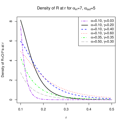
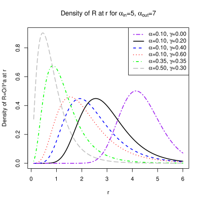
Figure 1. The density $f_{R}(r)$ for $(\alpha_{\text{i}n},\alpha_{\text{o}ut})=(7,5)$ (left) and $(\alpha_{\text{i}n},\alpha_{\text{o}ut})=(5,7)$ (right) for various values of $\alpha,\gamma$.

Additionally, we employ two numerical strategies based on the convergence of the conditional distribution of $O/I^{a}$ given $I>m$ as $m\to\infty$. Strategy 1 simulates a network of $10^{6}$ nodes using software provided by James Atwood (University of Massachusetts, Amherst) and then computes the histogram of $O/I^{a}$ for nodes whose in-degree $I$ exceeds some large threshold $m$. For the network simulation illustration, we chose $m$ to be the $99.95\%$ quantile of the in-degrees. Strategy 2 computes $p_{ij}$ on a grid $(i,j)$ using the recursion given in (3.4) and then estimates the density of $O/I^{a}$ using only the grid points with $i$ larger than $m$, the $m$ chosen to be the same value as used for the network simulation.

We observe from Figure 1 that the mode of $f_{R}(r)$ can drift away from the origin depending on parameter values. So we transform $R$ using the $\arctan$ function which gives all plots the same compact support $[0,\pi/2]$, instead of an infinite domain as in Figure 1. We compare the density of $R$ with the histogram based on network simulation and the density approximation provided by iteration across varying sets of parameter values. The density of $\arctan R$ with the plots from the alternative strategies based on simulation and iteration are displayed in Figure 2 for various choices of $(\delta_{\text{i}n},\delta_{\text{o}ut})$, with $\alpha=\beta=0.5$ and $\gamma=0$. For these parameter choices, the plots of the theoretical density with those resulting from network simulation and probability iteration are in good agreement.

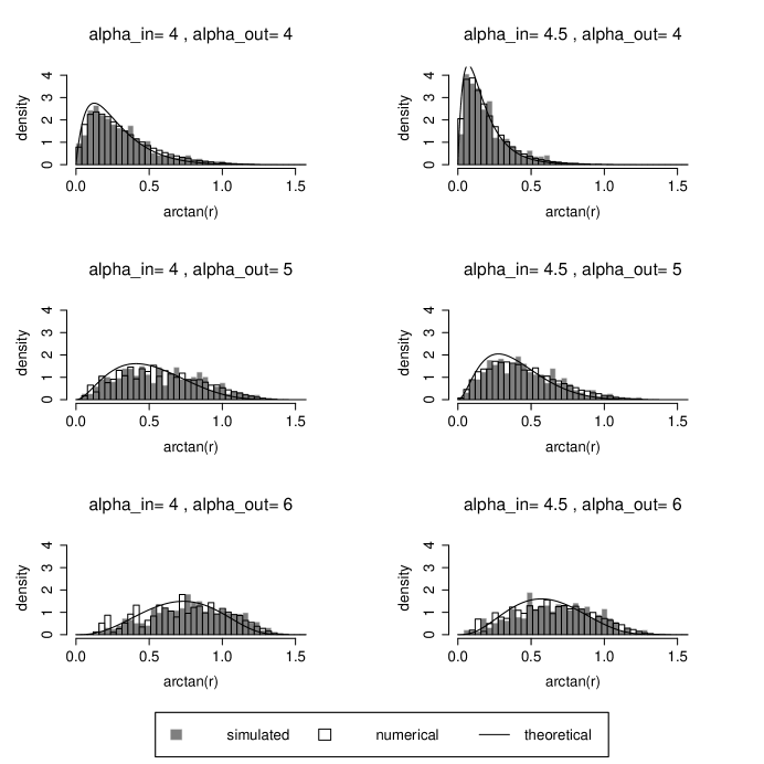
Figure 2. Comparison of the true density with the estimated densities of $\arctan R$ over various values of $(\alpha_{\text{i}n},\alpha_{\text{o}ut})$.

4.1.2. Density of the angular measure

A traditional way to describe the asymptotic dependence structure of a standardized heavy tailed vector is by using the angular measure. We transform the standardized vector $(I^{a},O)\mapsto\bigl{(}\arctan(O/I^{a}),\sqrt{O^{2}+I^{2a}}\bigr{)}$ to polar coordinates and then the distribution of $\arctan(O/I^{a})$ given $O^{2}+I^{2a}>m$, converges as $m\to\infty$ to the distribution to a random variable $\Theta$. The distribution of $\Theta$ is called the angular measure. The density of $\Theta$ can be calculated from Theorem 2 in a similar fashion as in Corollory 4 and is given by

$$f_{\Theta}(\theta) \propto \frac{\gamma}{\delta_{\text{i}n}}(\cos\theta)^{\frac{\delta_{\text{i}n}}{a}+\frac{1}{a}-1}(\sin\theta)^{\delta_{\text{o}ut}-1}\int_{0}^{\infty}t^{c_{1}^{-1}+\delta_{\text{i}n}+a\delta_{\text{o}ut}}e^{-t(\cos\theta)^{\frac{1}{a}}-t^{a}\sin\theta}\,dt\,$$

$$+\,\frac{\alpha}{\delta_{\text{o}ut}}(\cos\theta)^{\frac{\delta_{\text{i}n}}{a}-1}(\sin\theta)^{\delta_{\text{o}ut}}\int_{0}^{\infty}t^{a-1+c_{1}^{-1}+\delta_{\text{i}n}+a\delta_{\text{o}ut}}e^{-t(\cos\theta)^{\frac{1}{a}}-t^{a}\sin\theta}\,dt\,.$$

Two density approximations for the spectral density using network simulation and numerical iteration of the $p_{ij}$ are obtained in the same way as in Section 4.1.1. Using the same sets of parameters values as in Figure 2, we overlay the density approximations with the theoretical density in Figure 3. The truncation level was the $99.95\%$ percentile of $O^{2}+I^{2a}$. The agreement between the theoretical and estimated densities is quite good across the range of parameter values used.

The main difference between Figures 2 and 3 is the choice of conditioning set. In the first, $I^{a}$ was conditioned to be large, while in the second the sum of squares of the in- and out-degrees ($I^{2a}+O^{2}$) was conditioned to be large. Since the latter conditioning set is bigger and allows for the case that the in-degree is small relative to the out-degree, the density function in a neighborhood 0 will have less weight in Figure 3 than Figure 2.

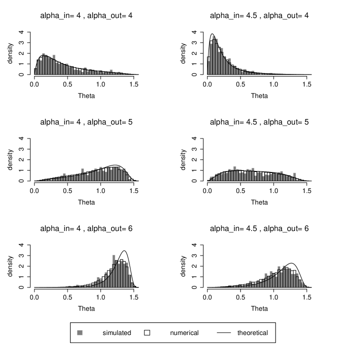
Figure 3. Comparison of the true angular density with estimates for various values of $(\alpha_{\text{i}n},\alpha_{\text{o}ut})$.

References

• Bollobás et al. (2003) B. Bollobás, C. Borgs, J. Chayes and O. Riordan (2003): Directed scale-free graphs. In Proceedings of the Fourteenth Annual ACM-SIAM Symposium on Discrete Algorithms (Baltimore, 2003). ACM, New York, pp. 132–139.
• Jones (1971) F. Jones (1971): Partial Differential Equations. Springer-Verlag, New York.
• Krapivsky and Redner (2001) P. Krapivsky and S. Redner (2001): Organization of growing random networks. Physical Review E 63:066123:1–14.
• Lindskog et al. (2013) F. Lindskog, S. Resnick and J. Roy (2013): Regularly Varying Measures on Metric Spaces: Hidden Regular Variation and Hidden Jumps. Technical report, School of ORIE, Cornell University. Preprint. Available at: http://arxiv.org/abs/1307.5803.
• Loève (1977) M. Loève (1977): Probability Theory, volume 1. Springer-Verlag, New York.
• Maulik et al. (2002) K. Maulik, S. Resnick and H. Rootzen (2002): Asymptotic independence and a network traffic model. Journal of Applied Probability 39:671–699.
• Resnick (2007) S. Resnick (2007): Heavy-Tail Phenomena: Probabilistic and Statistical Modeling. Springer, New York.