Variable Flavor Number Scheme for Final State Jets in Thrust

Piotr Pietrulewicz Fakultät für Physik, Universität Wien, Boltzmanngasse 5, 1090 Vienna, Austria    Simon Gritschacher Mathematical Institute, University of Oxford, Woodstock Road, Oxford, OX2 6GG, United Kingdom    Andre H. Hoang Fakultät für Physik, Universität Wien, Boltzmanngasse 5, 1090 Vienna, Austria Erwin Schrödinger International Institute for Mathematical Physics, University of Vienna, Boltzmanngasse 9, A-1090 Vienna, Austria    Ilaria Jemos Fakultät für Physik, Universität Wien, Boltzmanngasse 5, 1090 Vienna, Austria    Vicent Mateu Fakultät für Physik, Universität Wien, Boltzmanngasse 5, 1090 Vienna, Austria
Abstract

We present results for mass effects coming from secondary radiation of heavy quark pairs related to gluon splitting in the thrust distribution for e+esuperscript𝑒superscript𝑒e^{+}\,e^{-} collisions. The results are given in the dijet limit where the hard interaction scale and the scales related to collinear and soft radiation are widely separated. We account for the corresponding fixed-order corrections at 𝒪(αs2)𝒪superscriptsubscript𝛼𝑠2\mathcal{O}(\alpha_{s}^{2}) and the summation of all logarithmic terms related to the hard, collinear and soft scales as well as the quark mass at N3LL order. We also remove the 𝒪(ΛQCD)𝒪subscriptΛQCD{\cal O}(\Lambda_{\rm QCD}) renormalon in the partonic soft function leading to an infrared evolution equation with a matching condition related to the massive quark threshold. The quark mass can be arbitrary, ranging from the infinitely heavy case, where decoupling takes place, down to the massless limit where the results smoothly merge into the well-known predictions for massless quarks. Our results are formulated in the framework of factorization theorems for e+esuperscript𝑒superscript𝑒e^{+}\,e^{-} dijet production and provide universal threshold corrections for the renormalization group evolution of the hard current, the jet and soft functions at the scale where the massive quarks are integrated out. The results represent a first explicit realization of a variable flavor number scheme for final state jets along the lines of the well-known flavor number dependent evolution of the strong coupling αssubscript𝛼𝑠\alpha_{s} and the parton distribution functions.

preprint: UWTHPH 2014-07

I Introduction

The systematic theoretical treatment of mass effects in collider observables represents an important area in collider phenomenology where substantial progress is required to take full advantage of present and upcoming data. This concerns in particular the mass of the top quark Juste:2013dsa ; Jung:2013vpa ; Agashe:2013hma affecting physics at the Large Hadron Collider (LHC) and at a potential future linear collider, but also the masses of lighter heavy quarks such as charm Alekhin:2012vu ; Abramowicz:1900rp ; Kovarik:2012te and bottom quarks Campbell:2013qaa relevant e.g. in deep-inelastic scattering and event shape analyses at LEP. In this context examinations for the top quark may also be considered as study cases for the treatment of new massive colored particles that might be discovered in the near future. For inclusive cross sections at hadron colliders a systematic approach to treat massive quarks from the large mass limit, where decoupling takes place, continuously down to the small mass limit, where the description for massless quarks is approached, has been provided by Aivazis, Collins, Olness and Tung (ACOT) Aivazis:1993pi ; Aivazis:1993kh . Their work laid the basis of a variable flavor number scheme (VFNS) for inclusive processes in hadron collisions which, depending on the size of the quark mass in relation to the hard scattering and hadronization scales, allows one to factorize infrared-safe quark mass dependent hard coefficient corrections from flavor number dependent low-energy parton distribution functions. Since the concepts behind the work of ACOT are founded in the separation of close-to-mass-shell and off-shell modes, their approach is along the lines of effective field theory methods such as Soft-Collinear Effective Theory (SCET) Bauer:2000ew ; Bauer:2000yr and can be readily incorporated into it.

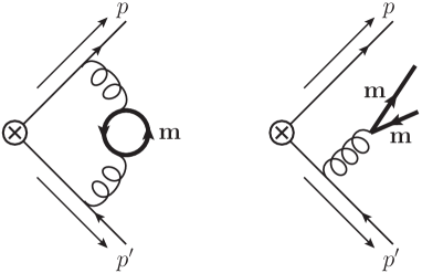
In this paper we present results for a VFNS for final state jets which are initiated by massless quarks and where massive quarks are produced through the radiation of gluons that split into a massive quark-antiquark pair, see Fig. 1. We call this type of heavy quark production mechanism secondary in contrast to the case where the massive quarks are produced directly in the hard current interaction, which we call primary. As for the VFNS scheme for inclusive processes in hadron collisions the approach is valid from the large mass limit, where the heavy quark decouples, continuously down to the small mass limit, where the predictions approach the known results for massless quarks. As a concrete application used to discuss the results we consider the secondary massive quark effects in the e+esuperscript𝑒superscript𝑒e^{+}\,e^{-} thrust distribution, where we define the thrust variable τ𝜏\tau via

τ= 1T= 1i|npi|jEj= 1i|npi|Q.𝜏1𝑇1subscript𝑖𝑛subscript𝑝𝑖subscript𝑗subscript𝐸𝑗1subscript𝑖𝑛subscript𝑝𝑖𝑄\displaystyle\tau\,=\,1-T\,=\,1-\,\frac{\sum_{i}|\vec{n}\cdot\vec{p}_{i}|}{\sum_{j}E_{j}}\,=\,1-\sum_{i}\frac{|\vec{n}\cdot\vec{p}_{i}|}{Q}\,. (1)

Here n𝑛\vec{n} is the thrust axis, and the sum is performed over all final state particles with momenta pisubscript𝑝𝑖\vec{p}_{i} and energies Eisubscript𝐸𝑖E_{i}. 111We define the thrust variable τ𝜏\tau normalized with respect to the c.m. energy Q𝑄Q, which is the sum of all energies and also agrees with the variable 2-jettiness Stewart:2010tn . In the dijet limit where τ𝜏\tau is small, the final state is governed by two narrow back-to-back jets and the scales of the hard interaction (Qsimilar-toabsent𝑄\sim Q), of collinear radiation (Qλsimilar-toabsent𝑄𝜆\sim Q\lambda) and of soft radiation (Qλ2similar-toabsent𝑄superscript𝜆2\sim Q\lambda^{2}) are widely separated (with λmax{τ1/2,(ΛQCD/Q)1/2}similar-to𝜆maxsuperscript𝜏12superscriptsubscriptΛQCD𝑄12\lambda\sim{\rm max}\{\tau^{1/2},(\Lambda_{\rm QCD}/Q)^{1/2}\}). In this context the dominant perturbative contributions in the thrust distribution for massless quarks are related to distributions in τ𝜏\tau and can be factorized into a hard coefficient function, a universal jet function and a soft function, all of which are defined in a gauge-invariant way. The latter has also a nonperturbative component which can be parametrized through a convolution with a soft model function that can be determined through fits to experimental data in a way free of 𝒪(ΛQCD)𝒪subscriptΛQCD\mathcal{O}(\Lambda_{\rm QCD}) renormalons Hoang:2007vb . The logarithmic terms within the dominant contributions can be summed using the anomalous dimensions of the hard coefficient and the jet and soft functions.

Accounting for quark masses in this context adds another non-trivial twist to the factorization setup since quark masses represent additional scales that can in principle have any hierarchy with respect to the hard, collinear and soft scales, which themselves depend on the value of τ𝜏\tau. 222Here we do not account for the effects of hadron masses (see Ref. Mateu:2012nk ). The possible relations among these scales can therefore vary substantially even within a single thrust distribution for a fixed c.m. energy Q𝑄Q. Within the factorization formalism the non-vanishing value of the quark mass can lead to a flavor number dependent renormalization group (RG) evolution, to threshold corrections in the evolution when crossing the quark mass scale and to additional mass-dependent fixed-order corrections in the hard coefficient and the jet and soft functions. The conceptual setup to define these quark mass dependent corrections is partially guided by identifying terms that are singular in the quark mass (in the small mass limit). The framework of SCET – properly extended to account for massive quarks – provides a natural framework to carry out this task systematically.
Refer to caption
Figure 1: Diagrams at 𝒪(αs2)𝒪superscriptsubscript𝛼𝑠2\mathcal{O}(\alpha_{s}^{2}) for virtual and real secondary radiation of massive quark pairs in primary massless quark production.
Refer to caption
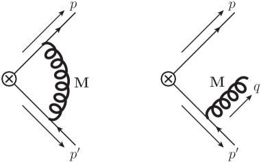
Figure 2: Diagrams at 𝒪(αs)𝒪subscript𝛼𝑠\mathcal{O}(\alpha_{s}) for virtual and real secondary radiation of gluons with mass M𝑀M in primary massless quark production.
Refer to caption
Figure 3: Figure illustrating the dispersion method for the vacuum polarization correction to the gluon propagator in the subtracted version with Π(q2=0)=0Πsuperscript𝑞200\Pi(q^{2}=0)=0 suitable for situations where the massive quark is not contributing to the renormalization group evolution. The explicit analytic form of the dispersion relations is discussed in Sec. IV.1.

The approach we propose is based on the seminal paper in Ref. Gritschacher:2013pha where it has been shown that the problem of secondary heavy quark production in the thrust distribution is closely related to the production of massive gauge bosons, see Fig. 2. The connection between these apparently different problems is related to the fact that the off-shell intermediate gluon that splits into the massive quark pair has an invariant mass that is bounded from below by twice the quark mass. So concerning the setup of the field theoretic modes needed to construct effective field theories for the various possible scenarios (related to the possible hierarchies with respect to the hard, collinear, soft and mass scales) both problems are quite similar since each of the field theoretic formulations has to account for (collinear and/or soft) gluonic modes with a finite typical invariant mass. In Ref. Gritschacher:2013pha we have discussed in detail the field theoretic scenarios to treat all possible hierarchies involving the “gluon mass” and the hard, collinear and soft scales, and we have provided the resulting form of the factorization theorems accounting for the required mass corrections, the changes of the RG evolution above and below the mass scale and the associated threshold corrections at the mass scale (“mass mode method”). At this level, replacing the gluonic modes by massive quark modes at 𝒪(αs2)𝒪superscriptsubscript𝛼𝑠2\mathcal{O}(\alpha_{s}^{2}) can be computationally more challenging, but does not lead to any additional conceptual complication. It was pointed out in Ref. Gritschacher:2013pha that for situations where the produced massive quark and antiquark enter a quantity coherently (i.e. only the sum of their momenta is relevant in the observable) one can obtain the corresponding 𝒪(αs2)𝒪superscriptsubscript𝛼𝑠2\mathcal{O}(\alpha_{s}^{2}) massive quark corrections from the 𝒪(αs)𝒪subscript𝛼𝑠\mathcal{O}(\alpha_{s}) “massive gluon” result using a dispersion integration as illustrated in Fig. 3. It was in particular demonstrated in Ref. Gritschacher:2013pha that also the conceptual issues involving the so-called rapidity divergences, which are related to specific divergences of collinear and soft modes with the same typical invariant mass, and the soft-bin subtractions, which avoid double counting between collinear and soft mass modes, can be dealt with at the level of the massive gluon results. As was shown in Ref. Gritschacher:2013tza , this computational trick can be also very useful for quantities where the quark and antiquark enter independently as the dispersion integral might already give the bulk of the numerical effects.

The VFNS we propose in this paper is presented and discussed on the basis of the secondary massive quark effects in the e+esuperscript𝑒superscript𝑒e^{+}\,e^{-} thrust distribution at N3LL order in the conventional SCET counting. 333At N3LL, one uses 4-loop cusp and 3-loop noncusp anomalous dimensions and 2-loop matrix elements and matching conditions. Concerning a recent thrust distribution analysis based on the SCET factorization theorem for massless quarks Abbate:2010xh the dominant secondary massive quark effects come from bottom quarks and represent minor corrections, since that analysis was carried out with data where the bottom quark mass effects are small due to restrictions in the values of the c.m. energy Q𝑄Q and the fit range in τ𝜏\tau. 444 In Ref. Abbate:2010xh some effects arising from the finite bottom mass related to primary production were accounted for, but none related to secondary bottom quark production. In general, however, the effects from secondary massive quarks are sizeable for lower Q𝑄Q values or τ𝜏\tau values in the peak and extreme dijet regions where the cross section depends strongly on the thrust value. Nevertheless, we consider the presentation of the VFNS given in this work primarily as a non-trivial showcase of the method which might serve as a guideline to apply the method to other problems involving final state jets.

The content of this work is as follows: In Sec. II we review the notations and the massless thrust factorization theorem with an emphasis on the corrections related to the number of massless quarks nfsubscript𝑛𝑓n_{\!f}. In Sec. III we briefly summarize the four relevant field theory scenarios needed to describe the possible hierarchies of the quark mass w.r. to the hard, jet and soft scales. We describe the respective factorization theorems, which are analogous to the ones given in Ref. Gritschacher:2013pha for the case of the “massive gluon”. We show explicitly the results of the 𝒪(αs2CFTF)𝒪superscriptsubscript𝛼𝑠2subscript𝐶𝐹subscript𝑇𝐹{\cal O}(\alpha_{s}^{2}C_{\!F}T_{F}) massive quark corrections to the hard, jet and soft functions including the results for the subtractions of 𝒪(ΛQCD)𝒪subscriptΛQCD{\cal O}(\Lambda_{\rm QCD}) renormalon contributions in the soft function using the gap scheme Hoang:2007vb ; Hoang:2008fs and the threshold corrections that arise when the RG evolution of the hard current coefficient, the jet and soft functions, as well as the gap parameter cross the massive quark pair flavor threshold. In Sec. IV we describe the computation of the 𝒪(αs2CFTF)𝒪superscriptsubscript𝛼𝑠2subscript𝐶𝐹subscript𝑇𝐹{\cal O}(\alpha_{s}^{2}C_{\!F}T_{F}) massive quark corrections to the hard and jet functions, which were the remaining unknown ingredients in the factorization theorems at this order. In Sec. V we show that the massive threshold corrections are directly related to the matrix elements in the factorization theorems in different renormalization schemes. This will also illustrate that at the conceptual level a separation into four different effective field theories is in principle not necessary and that the factorization theorems merge continuously into each other. Furthermore, we explain in this section how the freedom to set up the RG evolution leads to consistency conditions among the various threshold corrections underlining their universality. Finally, the results of this paper allow us to predict the singular 𝒪(αs2CFTF)𝒪superscriptsubscript𝛼𝑠2subscript𝐶𝐹subscript𝑇𝐹\mathcal{O}(\alpha_{s}^{2}C_{\!F}T_{F}) fixed-order corrections arising from secondary massive quarks, which to our knowledge have not been given in an explicit form in the literature before. In Sec. VI we carry out a numerical analysis at N3LL order for secondary massive bottom and top quarks at different c.m. energies. In particular we investigate the size of the mass corrections compared to the massless limit which turn out to be small in the tail region, but essential at the peak. Finally, Sec. VII contains our conclusions.

II The Massless Factorization Theorem for Thrust

In this section we briefly review the known massless factorization theorem for the most singular contributions of the thrust distribution in the dijet limit, which are the dominant terms for small values of τ𝜏\tau. The main purpose of this section is to set up the notations and to collect the perturbative results at 𝒪(αs2CFTF)𝒪superscriptsubscript𝛼𝑠2subscript𝐶𝐹subscript𝑇𝐹\mathcal{O}(\alpha_{s}^{2}C_{\!F}T_{F}) for later comparison and reference concerning the massive quark contributions discussed in later sections. Due to consistency the massive quark results must yield the massless expressions for vanishing quark mass. The factorization theorem for nfsubscript𝑛𝑓n_{\!f} massless quark flavors reads Korchemsky:1999kt ; Schwartz:2007ib ; Fleming:2007qr

1σ0dσdτ=Q|C(nf)(Q,μH)|2|UC(nf)(Q,μH,μ)|21subscript𝜎0d𝜎d𝜏𝑄superscriptsuperscript𝐶subscript𝑛𝑓𝑄subscript𝜇𝐻2superscriptsubscriptsuperscript𝑈subscript𝑛𝑓𝐶𝑄subscript𝜇𝐻𝜇2\displaystyle\frac{1}{\sigma_{0}}\frac{\mathrm{d}\sigma}{\mathrm{d}\tau}\,=\,Q\,\big{|}C^{(n_{\!f})}(Q,\mu_{H})\big{|}^{2}\,\big{|}U^{(n_{\!f})}_{C}(Q,\mu_{H},\mu)\big{|}^{2}
×dsdsJ(nf)(s,μJ)UJ(nf)(ss,μ,μJ)\displaystyle\times\int\!\mathrm{d}s\!\int\!\mathrm{d}s^{\prime}\,J^{(n_{\!f})}(s^{\prime},\mu_{J})\,U^{(n_{\!f})}_{J}(s-s^{\prime},\mu,\mu_{J})
×dS(nf)(QτsQ,μS)US(nf)(,μ,μS),\displaystyle\times\int\!\mathrm{d}\ell\,S^{(n_{\!f})}\Big{(}Q\,\tau-\frac{s}{Q}-\ell,\mu_{S}\Big{)}U^{(n_{\!f})}_{S}(\ell,\mu,\mu_{S})\,, (2)

where σ0subscript𝜎0\sigma_{0} denotes the total partonic e+esuperscript𝑒superscript𝑒e^{+}e^{-} cross-section at tree-level, C(nf)(Q,μ)superscript𝐶subscript𝑛𝑓𝑄𝜇C^{(n_{\!f})}(Q,\mu) is the hard current matching condition, J(nf)(s,μ)superscript𝐽subscript𝑛𝑓𝑠𝜇J^{(n_{\!f})}(s,\mu) the thrust jet function and S(nf)(,μ)superscript𝑆subscript𝑛𝑓𝜇S^{(n_{\!f})}(\ell,\mu) the thrust soft function. The terms UC(nf)subscriptsuperscript𝑈subscript𝑛𝑓𝐶U^{(n_{\!f})}_{C}, UJ(nf)subscriptsuperscript𝑈subscript𝑛𝑓𝐽U^{(n_{\!f})}_{J} and US(nf)subscriptsuperscript𝑈subscript𝑛𝑓𝑆U^{(n_{\!f})}_{S} are the RG evolution factors for the hard current matching, the jet and the soft functions, respectively. The superscript (nf)subscript𝑛𝑓(n_{\!f}) indicates that the MS¯¯MS\overline{\rm MS} scheme with nfsubscript𝑛𝑓n_{\!f} dynamic quark flavors is used for all renormalized quantities, as common when heavy quarks are not involved.

The functions C(nf)superscript𝐶subscript𝑛𝑓C^{(n_{\!f})}, J(nf)superscript𝐽subscript𝑛𝑓J^{(n_{\!f})} and S(nf)superscript𝑆subscript𝑛𝑓S^{(n_{\!f})} depend implicitly on nfsubscript𝑛𝑓n_{\!f} at 𝒪(αs)𝒪subscript𝛼𝑠\mathcal{O}(\alpha_{s}) through the strong coupling constant. The explicit dependence on nfsubscript𝑛𝑓n_{\!f} starts at 𝒪(αs2)𝒪superscriptsubscript𝛼𝑠2\mathcal{O}(\alpha_{s}^{2}). The expansion of the hard current matching coefficient up to this order has the form

C(nf)(Q,μ)=1+C(nf,1)(Q,μ)+[CCF(nf,2)(Q,μ)\displaystyle C^{(n_{\!f})}(Q,\mu)=1+C^{(n_{\!f},1)}(Q,\mu)+\Big{[}C^{(n_{\!f},2)}_{C_{\!F}}(Q,\mu)
+CCA(nf,2)(Q,μ)+Cnf(nf,2)(Q,μ)]+𝒪(αs3),\displaystyle+C^{(n_{\!f},2)}_{C_{\!A}}(Q,\mu)+C^{(n_{\!f},2)}_{n_{\!f}}(Q,\mu)\Big{]}+\mathcal{O}(\alpha_{s}^{3})\,, (3)

where C(nf,1)superscript𝐶subscript𝑛𝑓1C^{(n_{\!f},1)}, CCF(nf,2)subscriptsuperscript𝐶subscript𝑛𝑓2subscript𝐶𝐹C^{(n_{\!f},2)}_{C_{\!F}}, CCA(nf,2)subscriptsuperscript𝐶subscript𝑛𝑓2subscript𝐶𝐴C^{(n_{\!f},2)}_{C_{\!A}}, Cnf(nf,2)subscriptsuperscript𝐶subscript𝑛𝑓2subscript𝑛𝑓C^{(n_{\!f},2)}_{n_{\!f}} denote the contributions at 𝒪(αs)𝒪subscript𝛼𝑠\mathcal{O}(\alpha_{s}), 𝒪(αs2CF2)𝒪superscriptsubscript𝛼𝑠2superscriptsubscript𝐶𝐹2\mathcal{O}(\alpha_{s}^{2}C_{\!F}^{2}), 𝒪(αs2CFCA)𝒪superscriptsubscript𝛼𝑠2subscript𝐶𝐹subscript𝐶𝐴\mathcal{O}(\alpha_{s}^{2}C_{\!F}C_{\!A}), 𝒪(αs2CFTFnf)𝒪superscriptsubscript𝛼𝑠2subscript𝐶𝐹subscript𝑇𝐹subscript𝑛𝑓\mathcal{O}(\alpha_{s}^{2}C_{\!F}T_{F}n_{\!f}), respectively. We use the analogous notation for J(nf)superscript𝐽subscript𝑛𝑓J^{(n_{\!f})} and S(nf)superscript𝑆subscript𝑛𝑓S^{(n_{\!f})} as well as for all other perturbative expressions throughout this work. The additional dependence on a finite quark mass will be indicated in the arguments.

The massless current matching coefficient C(nf)(Q,μ)superscript𝐶subscript𝑛𝑓𝑄𝜇C^{(n_{\!f})}(Q,\mu) is determined by matching SCET to QCD. The renormalized contribution at 𝒪(αs2CFTF)𝒪superscriptsubscript𝛼𝑠2subscript𝐶𝐹subscript𝑇𝐹\mathcal{O}(\alpha_{s}^{2}C_{\!F}T_{F}) reads Matsuura (αs(nf)αs(nf)(μ)superscriptsubscript𝛼𝑠subscript𝑛𝑓superscriptsubscript𝛼𝑠subscript𝑛𝑓𝜇\alpha_{s}^{(n_{\!f})}\equiv\alpha_{s}^{(n_{\!f})}(\mu))

Cnf(nf,2)(Q,μ)=(αs(nf))2CFTFnf16π2{49LQ3+389LQ2\displaystyle C^{(n_{\!f},2)}_{n_{\!f}}(Q,\mu)=\frac{\big{(}\alpha_{s}^{(n_{\!f})}\big{)}^{2}C_{\!F}T_{F}n_{\!f}}{16\pi^{2}}\left\{-\,\frac{4}{9}\,L_{-Q}^{3}+\frac{38}{9}\,L_{-Q}^{2}\right.
(41827+4π29)LQ+4085162+23π227+49ζ3},\displaystyle\left.-\,\bigg{(}\frac{418}{27}+\frac{4\pi^{2}}{9}\bigg{)}L_{-Q}+\frac{4085}{162}+\frac{23\pi^{2}}{27}+\frac{4}{9}\,\zeta_{3}\right\}\,, (4)

where LQ=ln(Q2/μ2)subscript𝐿𝑄lnsuperscript𝑄2superscript𝜇2L_{-Q}=\textrm{ln}{(-Q^{2}/\mu^{2})} (with Q2Q2+i 0superscript𝑄2superscript𝑄2𝑖 0Q^{2}\equiv Q^{2}+i\,0). The associated contributions to the current renormalization factor read

ZC,nf(nf,2)(Q,μ)=(αs(nf))2CFTFnf16π2{2ϵ3\displaystyle Z^{(n_{\!f},2)}_{C,n_{\!f}}(Q,\mu)=\frac{\big{(}\alpha_{s}^{(n_{\!f})}\big{)}^{2}C_{\!F}T_{F}n_{\!f}}{16\pi^{2}}\left\{\!-\,\frac{2}{\epsilon^{3}}\right. (5)
+1ϵ2[43LQ89]+1ϵ[209LQ+6527+π23]}.\displaystyle+\left.\frac{1}{\epsilon^{2}}\left[\frac{4}{3}\,L_{-Q}-\frac{8}{9}\right]+\frac{1}{\epsilon}\left[-\,\frac{20}{9}\,L_{-Q}+\frac{65}{27}+\frac{\pi^{2}}{3}\right]\right\}\,.

The jet function is given by a vacuum correlator of two jet fields in SCET and describes the collinear dynamics of the two back-to-back jets. The renormalized expression for J(nf)(s,μ)superscript𝐽subscript𝑛𝑓𝑠𝜇J^{(n_{\!f})}(s,\mu) at 𝒪(αs2CFTF)𝒪superscriptsubscript𝛼𝑠2subscript𝐶𝐹subscript𝑇𝐹\mathcal{O}(\alpha_{s}^{2}C_{\!F}T_{F}) reads Becher:2006qw

μ2Jnf(nf,2)(s,μ)=(αs(nf))2CFTFnf16π2{[405781\displaystyle\mu^{2}J^{(n_{\!f},2)}_{n_{\!f}}(s,\mu)=\frac{\big{(}\alpha_{s}^{(n_{\!f})}\big{)}^{2}C_{\!F}T_{F}n_{\!f}}{16\pi^{2}}\left\{\left[-\,\frac{4057}{81}\right.\right.
+136π227+329ζ3]δ(s¯)+(9882716π29)[θ(s¯)s¯]+\displaystyle+\left.\frac{136\pi^{2}}{27}+\frac{32}{9}\,\zeta_{3}\right]\!\delta(\bar{s})+\left(\frac{988}{27}-\frac{16\pi^{2}}{9}\right)\!\left[\frac{\theta(\bar{s})}{\bar{s}}\right]_{+}
2329[θ(s¯)lns¯s¯]++163[θ(s¯)ln2s¯s¯]+},\displaystyle\left.-\frac{232}{9}\!\left[\frac{\theta(\bar{s})\textrm{ln}{\bar{s}}}{\bar{s}}\right]_{+}+\frac{16}{3}\!\left[\frac{\theta(\bar{s})\textrm{ln}^{2}{\bar{s}}}{\bar{s}}\right]_{+}\right\}\,, (6)

with s¯s/μ2¯𝑠𝑠superscript𝜇2\bar{s}\equiv s/\mu^{2}. The corresponding contributions to the renormalization factor read

μ2ZJ,nf(nf,2)(s,μ)=(αs(nf))2CFTFnf16π2{[8ϵ349ϵ2\displaystyle\mu^{2}Z^{(n_{\!f},2)}_{J,n_{\!f}}(s,\mu)=\frac{\big{(}\alpha_{s}^{(n_{\!f})}\big{)}^{2}C_{\!F}T_{F}n_{\!f}}{16\pi^{2}}\left\{\left[\frac{8}{\epsilon^{3}}-\frac{4}{9\epsilon^{2}}\right.\right. (7)
1ϵ(24227+4π29)]δ(s¯)(163ϵ2809ϵ)[θ(s¯)s¯]+}.\displaystyle\left.-\left.\frac{1}{\epsilon}\left(\frac{242}{27}+\frac{4\pi^{2}}{9}\right)\right]\!\delta(\bar{s})-\left(\frac{16}{3\epsilon^{2}}-\frac{80}{9\epsilon}\right)\!\left[\frac{\theta(\bar{s})}{\bar{s}}\right]_{+}\right\}\,.

The thrust soft function S(nf)(,μ)superscript𝑆subscript𝑛𝑓𝜇S^{(n_{\!f})}\left(\ell,\mu\right) describes ultrasoft radiation between the two jets. It can be written as a convolution of the partonic soft function describing perturbative corrections at the soft scale and the nonperturbative hadronic soft function Hoang:2007vb . The renormalized expression for the partonic soft function at 𝒪(αs2CFTF)𝒪superscriptsubscript𝛼𝑠2subscript𝐶𝐹subscript𝑇𝐹\mathcal{O}(\alpha_{s}^{2}C_{\!F}T_{F}) is Kelley:2011ng ; Monni:2011gb

μS^nf(nf,2)(,μ)=(αs(nf))2CFTFnf16π2{[8081+74π227\displaystyle\mu\,\hat{S}^{(n_{\!f},2)}_{n_{\!f}}(\ell,\mu)=\frac{\big{(}\alpha_{s}^{(n_{\!f})}\big{)}^{2}C_{\!F}T_{F}n_{\!f}}{16\pi^{2}}\left\{\left[\frac{80}{81}+\frac{74\pi^{2}}{27}\right.\right.
2329ζ3]δ(¯)+(44827+16π29)[θ(¯)¯]+\displaystyle-\left.\frac{232}{9}\,\zeta_{3}\right]\!\delta(\bar{\ell})+\left(-\,\frac{448}{27}+\frac{16\pi^{2}}{9}\right)\!\left[\frac{\theta(\bar{\ell})}{\bar{\ell}}\right]_{+}
+3209[θ(¯)ln¯¯]+643[θ(¯)ln2¯¯]+}.\displaystyle\left.+\,\frac{320}{9}\!\left[\frac{\theta(\bar{\ell})\textrm{ln}\,\bar{\ell}}{\bar{\ell}}\right]_{+}-\frac{64}{3}\!\left[\frac{\theta(\bar{\ell})\textrm{ln}^{2}{\bar{\ell}}}{\bar{\ell}}\right]_{+}\right\}\,. (8)

with ¯/μ¯𝜇\bar{\ell}\equiv\ell/\mu. The corresponding contributions to the renormalization factor read

μZS,nf(nf,2)(,μ)=(αs(nf))2CFTFnf16π2{[4ϵ3+209ϵ2\displaystyle\mu\,Z^{(n_{\!f},2)}_{S,n_{\!f}}(\ell,\mu)=\frac{\big{(}\alpha_{s}^{(n_{\!f})}\big{)}^{2}C_{\!F}T_{F}n_{\!f}}{16\pi^{2}}\left\{\left[-\,\frac{4}{\epsilon^{3}}+\frac{20}{9\epsilon^{2}}\right.\right. (9)
+1ϵ(112272π29)]δ(¯)+(163ϵ2809ϵ)[θ(¯)¯]+}.\displaystyle\left.+\left.\frac{1}{\epsilon}\left(\frac{112}{27}-\frac{2\pi^{2}}{9}\right)\right]\!\delta(\bar{\ell})+\left(\frac{16}{3\epsilon^{2}}-\frac{80}{9\epsilon}\right)\!\left[\frac{\theta(\bar{\ell})}{\bar{\ell}}\right]_{+}\right\}\,.

The overlap between the partonic and the nonperturbative contributions in dimensional regularization leads to an infrared sensitivity of the perturbative corrections implying factorially enhanced coefficients (“renormalon”). One can eliminate the renormalon problem for the leading 𝒪(ΛQCD)𝒪subscriptΛQCD{\cal O}(\Lambda_{\rm QCD}) power correction that arises in the operator production expansion (OPE) of the soft function for ΛQCDmuch-greater-thansubscriptΛQCD\ell\gg\Lambda_{\rm QCD} by introducing a gap parameter ΔΛQCDsimilar-toΔsubscriptΛQCD\Delta\sim\Lambda_{\rm QCD} in the hadronic soft model function related to a minimal hadronic energy deposit together with properly defined perturbative subtractions in the partonic soft function. This cancels the linear sensitivity to small momenta in the partonic soft function order-by-order in perturbation theory Hoang:2007vb ; Hoang:2008fs . The complete function including the renormalon subtractions has the form

S(nf)(,μ)=superscript𝑆subscript𝑛𝑓𝜇absent\displaystyle S^{(n_{\!f})}(\ell,\mu)= dS^(nf)(2δ(nf)(R,μ),μ)differential-dsuperscriptsuperscript^𝑆subscript𝑛𝑓superscript2superscript𝛿subscript𝑛𝑓𝑅𝜇𝜇\displaystyle\int\!\mathrm{d}\ell^{\prime}\,\hat{S}^{(n_{\!f})}\Big{(}\ell-\ell^{\prime}-2\,\delta^{(n_{\!f})}(R,\mu),\mu\Big{)}
×F(2Δ¯(nf)(R,μ)),absent𝐹superscript2superscript¯Δsubscript𝑛𝑓𝑅𝜇\displaystyle\times F\Big{(}\ell^{\prime}-2\,\bar{\Delta}^{(n_{\!f})}(R,\mu)\Big{)}\,, (10)

where δ(nf)(R,μ)superscript𝛿subscript𝑛𝑓𝑅𝜇\delta^{(n_{\!f})}(R,\mu) is the subtraction series, Δ¯(nf)(R,μ)superscript¯Δsubscript𝑛𝑓𝑅𝜇\bar{\Delta}^{(n_{\!f})}(R,\mu) is the gap parameter which is free of the 𝒪(ΛQCD)𝒪subscriptΛQCD\mathcal{O}(\Lambda_{\rm QCD}) renormalon and F𝐹F is the soft model function. A convenient definition for δ(nf)(R,μ)superscript𝛿subscript𝑛𝑓𝑅𝜇\delta^{(n_{\!f})}(R,\mu) with consistent RG properties has been given in Ref. Hoang:2008fs and has the form

δ(nf)(R,μ)=R2eγEddln(ix)lnS~(nf)(x,μ)|x=(iReγE)1,superscript𝛿subscript𝑛𝑓𝑅𝜇evaluated-at𝑅2superscript𝑒subscript𝛾𝐸ddln𝑖𝑥lnsuperscript~𝑆subscript𝑛𝑓𝑥𝜇𝑥superscript𝑖𝑅superscript𝑒subscript𝛾𝐸1\displaystyle\delta^{(n_{\!f})}(R,\mu)=\frac{R}{2}\,e^{\gamma_{E}}\frac{\mathrm{d}}{\mathrm{d}\,\textrm{ln}(ix)}\!\left.\textrm{ln}\,\tilde{S}^{(n_{\!f})}(x,\mu)\right|_{x=(iRe^{\gamma_{E}})^{-1}}\,, (11)

where S~(nf)superscript~𝑆subscript𝑛𝑓\tilde{S}^{(n_{\!f})} is the partonic soft function in configuration space, S~(nf)(x,μ)=dS^(nf)(,μ)eixsuperscript~𝑆subscript𝑛𝑓𝑥𝜇differential-dsuperscript^𝑆subscript𝑛𝑓𝜇superscript𝑒𝑖𝑥\tilde{S}^{(n_{\!f})}(x,\mu)=\int\mathrm{d}\ell\,\hat{S}^{(n_{\!f})}(\ell,\mu)\,e^{-i\ell x}. The 𝒪(αs2CFTF)𝒪superscriptsubscript𝛼𝑠2subscript𝐶𝐹subscript𝑇𝐹\mathcal{O}(\alpha_{s}^{2}C_{\!F}T_{F}) correction reads

δnf(nf,2)(R,μ)=(αs(nf))2CFTFnf16π2ReγE[83ln2(μ2R2)\displaystyle\delta^{(n_{\!f},2)}_{n_{\!f}}(R,\mu)=\frac{\big{(}\alpha_{s}^{(n_{\!f})}\big{)}^{2}C_{\!F}T_{F}n_{\!f}}{16\pi^{2}}\,R\,e^{\gamma_{E}}\!\left[\frac{8}{3}\,\textrm{ln}^{2}\bigg{(}\frac{\mu^{2}}{R^{2}}\bigg{)}\right.
+809ln(μ2R2)+22427+8π29].\displaystyle+\left.\frac{80}{9}\,\textrm{ln}\bigg{(}\frac{\mu^{2}}{R^{2}}\bigg{)}+\frac{224}{27}+\frac{8\pi^{2}}{9}\right]\,. (12)

The renormalon-free gap parameter Δ¯(nf)(R,μ)superscript¯Δsubscript𝑛𝑓𝑅𝜇\bar{\Delta}^{(n_{\!f})}(R,\mu) is related to the ambiguous, but scale-independent “bare” gap parameter ΔΔ\Delta by the relation555The “bare” gap parameter ΔΔ\Delta is conceptually analogous to the heavy quark pole mass parameter, so all renormalon-free gap schemes can be related to each other unambiguously through their relation to the bare ΔΔ\Delta. Frequently ΔΔ\Delta is also called the “MS¯¯MS\overline{\rm MS} gap parameter”.

Δ=Δ¯(nf)(R,μ)+δ(nf)(R,μ)Δsuperscript¯Δsubscript𝑛𝑓𝑅𝜇superscript𝛿subscript𝑛𝑓𝑅𝜇\displaystyle\Delta=\bar{\Delta}^{(n_{\!f})}(R,\mu)+\delta^{(n_{\!f})}(R,\mu)\, (13)

Thus Δ¯(nf)(R,μ)superscript¯Δsubscript𝑛𝑓𝑅𝜇\bar{\Delta}^{(n_{\!f})}(R,\mu) is scale- and subtraction scheme-dependent. The natural choice for the scale R𝑅R of the renormalon-free gap parameter is RΛQCDgreater-than-or-equivalent-to𝑅subscriptΛQCDR\gtrsim\Lambda_{\rm QCD}. On the other hand, the renormalon subtraction δ(nf)(R,μ)superscript𝛿subscript𝑛𝑓𝑅𝜇\delta^{(n_{\!f})}(R,\mu) should be evaluated for μ=μS𝜇subscript𝜇𝑆\mu=\mu_{S}, which is much larger than ΛQCDsubscriptΛQCD\Lambda_{\rm QCD} in the tail region, in order to achieve a proper cancellation with the IR sensitive terms in the soft function. This requires a resummation if the logarithm ln(μS/ΛQCD)lnsubscript𝜇𝑆subscriptΛQCD\textrm{ln}(\mu_{S}/\Lambda_{\rm QCD}) is large, which can be performed by solving the evolution equations Hoang:2007vb ; Hoang:2008yj ; Hoang:2009yr ; Hoang:2008fs

RddRΔ¯(nf)(R,R)𝑅dd𝑅superscript¯Δsubscript𝑛𝑓𝑅𝑅\displaystyle R\,\frac{\mathrm{d}}{\mathrm{d}R}\,\bar{\Delta}^{(n_{\!f})}(R,R) =RddRδ(nf)(R,R)absent𝑅dd𝑅superscript𝛿subscript𝑛𝑓𝑅𝑅\displaystyle=-\,R\,\frac{\mathrm{d}}{\mathrm{d}R}\,\delta^{(n_{\!f})}(R,R)
RγR(nf)[αs(nf)(R)],absent𝑅subscriptsuperscript𝛾subscript𝑛𝑓𝑅delimited-[]superscriptsubscript𝛼𝑠subscript𝑛𝑓𝑅\displaystyle\equiv-\,R\,\gamma^{(n_{\!f})}_{R}[\alpha_{s}^{(n_{\!f})}(R)]\,, (14)
μddμΔ¯(nf)(R,μ)𝜇dd𝜇superscript¯Δsubscript𝑛𝑓𝑅𝜇\displaystyle\mu\,\frac{\mathrm{d}}{\mathrm{d}\mu}\,\bar{\Delta}^{(n_{\!f})}(R,\mu) RγΔ,μ(nf)absent𝑅subscriptsuperscript𝛾subscript𝑛𝑓Δ𝜇\displaystyle\equiv-\,R\,\gamma^{(n_{\!f})}_{\Delta,\mu}
=2ReγEΓcusp(nf)[αs(nf)(μ)].absent2𝑅superscript𝑒subscript𝛾𝐸superscriptsubscriptΓcuspsubscript𝑛𝑓delimited-[]superscriptsubscript𝛼𝑠subscript𝑛𝑓𝜇\displaystyle=2\,R\,e^{\gamma_{E}}\Gamma_{\rm cusp}^{(n_{\!f})}[\alpha_{s}^{(n_{\!f})}(\mu)]\,. (15)

Note that the R-anomalous dimension γR(nf)subscriptsuperscript𝛾subscript𝑛𝑓𝑅\gamma^{(n_{\!f})}_{R}, which is responsible for relating Δ¯(nf)superscript¯Δsubscript𝑛𝑓\bar{\Delta}^{(n_{\!f})} at different values of R𝑅R to each other in a way free of the 𝒪(ΛQCD)𝒪subscriptΛQCD\mathcal{O}(\Lambda_{\rm QCD}) renormalon and free of large IR logarithms, happens to vanish at 𝒪(αs)𝒪subscript𝛼𝑠\mathcal{O}(\alpha_{s}). Thus the leading anomalous dimension at 𝒪(αs2)𝒪superscriptsubscript𝛼𝑠2\mathcal{O}(\alpha_{s}^{2}) depends both linearly and via the strong coupling constant on the number of active flavors nfsubscript𝑛𝑓n_{\!f}. The 𝒪(αs2CFTF)𝒪superscriptsubscript𝛼𝑠2subscript𝐶𝐹subscript𝑇𝐹\mathcal{O}(\alpha_{s}^{2}C_{\!F}T_{F}) contribution reads

γR,nf(nf,2)=(αs(nf))2CFTFnf16π2eγE(22427+8π29).subscriptsuperscript𝛾subscript𝑛𝑓2𝑅subscript𝑛𝑓superscriptsuperscriptsubscript𝛼𝑠subscript𝑛𝑓2subscript𝐶𝐹subscript𝑇𝐹subscript𝑛𝑓16superscript𝜋2superscript𝑒subscript𝛾𝐸224278superscript𝜋29\displaystyle\gamma^{(n_{\!f},2)}_{R,n_{\!f}}=\frac{\big{(}\alpha_{s}^{(n_{\!f})}\big{)}^{2}C_{\!F}T_{F}n_{\!f}}{16\pi^{2}}\,e^{\gamma_{E}}\!\left(\frac{224}{27}+\frac{8\pi^{2}}{9}\right). (16)

Note that the first moment of the soft model function 2Ω12subscriptΩ12\,\Omega_{1} also becomes a scheme- and scale-dependent quantity once we employ a renormalon-free gap scheme. The moment parameter Ω1(nf)(R,μ)subscriptsuperscriptΩsubscript𝑛𝑓1𝑅𝜇\Omega^{(n_{\!f})}_{1}(R,\mu) is then related to the gap parameter Δ¯(nf)(R,μ)superscript¯Δsubscript𝑛𝑓𝑅𝜇\bar{\Delta}^{(n_{\!f})}(R,\mu) via

Ω1(nf)(R,μ)subscriptsuperscriptΩsubscript𝑛𝑓1𝑅𝜇\displaystyle\Omega^{(n_{\!f})}_{1}(R,\mu) 120dF(2Δ¯(nf)(R,μ))absent12superscriptsubscript0differential-d𝐹2superscript¯Δsubscript𝑛𝑓𝑅𝜇\displaystyle\equiv\frac{1}{2}\int_{0}^{\infty}\!{\rm d}\ell\,\ell\,F\big{(}\ell-2\,\bar{\Delta}^{(n_{\!f})}(R,\mu)\big{)}
=Δ¯(nf)(R,μ)+120dF().absentsuperscript¯Δsubscript𝑛𝑓𝑅𝜇12superscriptsubscript0differential-d𝐹\displaystyle=\bar{\Delta}^{(n_{\!f})}(R,\mu)+\frac{1}{2}\int_{0}^{\infty}\!{\rm d}\ell\,\ell\,F(\ell)\,. (17)

Large logarithms between the characteristic scales of each sector, μHsubscript𝜇𝐻\mu_{H}, μJsubscript𝜇𝐽\mu_{J} and μSsubscript𝜇𝑆\mu_{S}, and the final, common renormalization scale of the factorization theorem μ𝜇\mu are summed by the evolution factors UC(nf)subscriptsuperscript𝑈subscript𝑛𝑓𝐶U^{(n_{\!f})}_{C}, UJ(nf)subscriptsuperscript𝑈subscript𝑛𝑓𝐽U^{(n_{\!f})}_{J} and US(nf)subscriptsuperscript𝑈subscript𝑛𝑓𝑆U^{(n_{\!f})}_{S}. They satisfy the RG equations

μddμUC(nf)(Q,μH,μ)𝜇dd𝜇subscriptsuperscript𝑈subscript𝑛𝑓𝐶𝑄subscript𝜇𝐻𝜇\displaystyle\mu\,\frac{\mathrm{d}}{\mathrm{d}\mu}\,U^{(n_{\!f})}_{C}(Q,\mu_{H},\mu)
=γC(nf)(Q,μ)UC(nf)(Q,μH,μ),absentsubscriptsuperscript𝛾subscript𝑛𝑓𝐶𝑄𝜇subscriptsuperscript𝑈subscript𝑛𝑓𝐶𝑄subscript𝜇𝐻𝜇\displaystyle=\gamma^{(n_{\!f})}_{C}(Q,\mu)\,U^{(n_{\!f})}_{C}(Q,\mu_{H},\mu)\,, (18)
μddμUJ(nf)(s,μ,μJ)𝜇dd𝜇subscriptsuperscript𝑈subscript𝑛𝑓𝐽𝑠𝜇subscript𝜇𝐽\displaystyle\mu\,\frac{\mathrm{d}}{\mathrm{d}\mu}\,U^{(n_{\!f})}_{J}(s,\mu,\mu_{J})
=dsγJ(nf)(ss,μ)UJ(nf)(s,μ,μJ),absentdifferential-dsuperscript𝑠subscriptsuperscript𝛾subscript𝑛𝑓𝐽𝑠superscript𝑠𝜇subscriptsuperscript𝑈subscript𝑛𝑓𝐽superscript𝑠𝜇subscript𝜇𝐽\displaystyle=\int\!\mathrm{d}s^{\prime}\,\gamma^{(n_{\!f})}_{J}(s-s^{\prime},\mu)\,U^{(n_{\!f})}_{J}(s^{\prime},\mu,\mu_{J})\,, (19)
μddμUS(nf)(,μ,μS)𝜇dd𝜇subscriptsuperscript𝑈subscript𝑛𝑓𝑆𝜇subscript𝜇𝑆\displaystyle\mu\,\frac{\mathrm{d}}{\mathrm{d}\mu}\,U^{(n_{\!f})}_{S}(\ell,\mu,\mu_{S})
=dγS(nf)(,μ)US(nf)(,μ,μS).absentdifferential-dsuperscriptsubscriptsuperscript𝛾subscript𝑛𝑓𝑆superscript𝜇subscriptsuperscript𝑈subscript𝑛𝑓𝑆superscript𝜇subscript𝜇𝑆\displaystyle=\int\!\mathrm{d}\ell^{\prime}\,\gamma^{(n_{\!f})}_{S}(\ell-\ell^{\prime},\mu)\,U^{(n_{\!f})}_{S}(\ell^{\prime},\mu,\mu_{S})\,. (20)

The evolution factors are already at LL sensitive to the number of active flavors nfsubscript𝑛𝑓n_{\!f} due to the running of αs(nf)superscriptsubscript𝛼𝑠subscript𝑛𝑓\alpha_{s}^{(n_{\!f})}. Thus, modifying the number of active quark flavors in the evolution affects the thrust distribution already at LL through its dependence on αssubscript𝛼𝑠\alpha_{s}, which happens when a mass threshold is crossed. The explicit dependence of the anomalous dimensions on nfsubscript𝑛𝑓n_{\!f} starts at 𝒪(αs2)𝒪superscriptsubscript𝛼𝑠2\mathcal{O}(\alpha_{s}^{2}), and the corresponding 𝒪(αs2CFTF)𝒪superscriptsubscript𝛼𝑠2subscript𝐶𝐹subscript𝑇𝐹\mathcal{O}(\alpha_{s}^{2}C_{\!F}T_{F}) terms read (Q2Q2+i 0superscript𝑄2superscript𝑄2𝑖 0Q^{2}\equiv Q^{2}+i\,0)

γC,nf(nf,2)(Q,μ)=(αs(nf))2CFTFnf16π2[Γnf(2)ln(Q2μ2)\displaystyle\gamma^{(n_{\!f},2)}_{C,n_{\!f}}(Q,\mu)=\frac{\big{(}\alpha_{s}^{(n_{\!f})}\big{)}^{2}C_{\!F}T_{F}n_{\!f}}{16\pi^{2}}\left[\Gamma^{(2)}_{n_{\!f}}\,\textrm{ln}\bigg{(}\!\!-\frac{Q^{2}}{\mu^{2}}\bigg{)}\right.
+26027+4π23],\displaystyle+\left.\frac{260}{27}+\frac{4\pi^{2}}{3}\right], (21)
μ2γJ,nf(nf,2)(s,μ)=(αs(nf))2CFTFnf16π2{ 4Γnf(2)[θ(s¯)s¯]+\displaystyle\mu^{2}\gamma^{(n_{\!f},2)}_{J,n_{\!f}}(s,\mu)=\frac{\big{(}\alpha_{s}^{(n_{\!f})}\big{)}^{2}C_{\!F}T_{F}n_{\!f}}{16\pi^{2}}\left\{\!-\,4\,\Gamma^{(2)}_{n_{\!f}}\left[\frac{\theta(\bar{s})}{\bar{s}}\right]_{+}\right.
(96827+16π29)δ(s¯)},\displaystyle-\left.\left(\frac{968}{27}+\frac{16\pi^{2}}{9}\right)\!\delta(\bar{s})\right\}, (22)
μγS,nf(nf,2)(,μ)=(αs(nf))2CFTFnf16π2{4Γnf(2)[θ(¯)¯]+\displaystyle\mu\gamma^{(n_{\!f},2)}_{S,n_{\!f}}(\ell,\mu)=\frac{\big{(}\alpha_{s}^{(n_{\!f})}\big{)}^{2}C_{\!F}T_{F}n_{\!f}}{16\pi^{2}}\left\{4\,\Gamma^{(2)}_{n_{\!f}}\left[\frac{\theta(\bar{\ell})}{\bar{\ell}}\right]_{+}\right.
+(448278π29)δ(¯)},\displaystyle+\left.\left(\frac{448}{27}-\frac{8\pi^{2}}{9}\right)\!\delta(\bar{\ell})\right\}, (23)

where Γnf(2)= 80/9subscriptsuperscriptΓ2subscript𝑛𝑓809\Gamma^{(2)}_{n_{\!f}}=-\,80/9 denotes the 𝒪(αs2CFTFnf)𝒪superscriptsubscript𝛼𝑠2subscript𝐶𝐹subscript𝑇𝐹subscript𝑛𝑓\mathcal{O}(\alpha_{s}^{2}C_{\!F}T_{F}n_{\!f}) coefficient of the cusp anomalous dimension Γcusp(nf)subscriptsuperscriptΓsubscript𝑛𝑓cusp\Gamma^{(n_{\!f})}_{{\rm cusp}}.

In Eq. (2) the choice of μ𝜇\mu is arbitrary, and the dependence on μ𝜇\mu cancels exactly working to any given order in perturbation theory. In the following we will present our results adopting the choice μ=μS𝜇subscript𝜇𝑆\mu=\mu_{S}, such that the evolution factor US(1)(,μS,μS)=δ()superscriptsubscript𝑈𝑆1subscript𝜇𝑆subscript𝜇𝑆𝛿U_{S}^{(1)}(\ell,\mu_{S},\mu_{S})=\delta(\ell) and can be dropped from Eq. (2). The fact that any other choice for μ𝜇\mu can be implemented leads to a consistency relation between the renormalization group factors Fleming:2007qr , which reads

Q|UC(nf)(Q,μ0,μ)|2UJ(nf)(Q,μ,μ0)=US(nf)(,μ0,μ).𝑄superscriptsuperscriptsubscript𝑈𝐶subscript𝑛𝑓𝑄subscript𝜇0𝜇2superscriptsubscript𝑈𝐽subscript𝑛𝑓𝑄𝜇subscript𝜇0superscriptsubscript𝑈𝑆subscript𝑛𝑓subscript𝜇0𝜇\displaystyle Q\,\big{|}U_{C}^{(n_{\!f})}(Q,\mu_{0},\mu)\big{|}^{2}\,U_{J}^{(n_{\!f})}(Q\ell,\mu,\mu_{0})=U_{S}^{(n_{\!f})}(\ell,\mu_{0},\mu)\,. (24)

It can also be written as a relation for the μ𝜇\mu-anomalous dimensions,

2Re[γC(nf)(Q,μ)]δ(¯)+QμγJ(nf)(Q,μ)=μγS(nf)(,μ).2Redelimited-[]subscriptsuperscript𝛾subscript𝑛𝑓𝐶𝑄𝜇𝛿¯𝑄𝜇superscriptsubscript𝛾𝐽subscript𝑛𝑓𝑄𝜇𝜇superscriptsubscript𝛾𝑆subscript𝑛𝑓𝜇\displaystyle 2\,{\rm Re}\big{[}\gamma^{(n_{\!f})}_{C}(Q,\mu)\big{]}\delta(\bar{\ell})+Q\,\mu\,\gamma_{J}^{(n_{\!f})}(Q\ell,\mu)=-\,\mu\,\gamma_{S}^{(n_{\!f})}(\ell,\mu). (25)

In the massive quark case this consistency relation remains intact since the UV divergences are mass independent. However, since the quark mass represents an additional relevant scale the factorization theorem exhibits a richer structure due to the increased number of scales, and additional consistency relations emerge.

III Mass Mode Setup and Summary of Results

In this section we briefly review the mass mode setup of Ref. Gritschacher:2013pha , which is based on four different effective field theory scenarios associated to the hierarchies between the hard, jet and soft scales and the quark mass. We also discuss the form of the resulting factorization theorems and present the final results for all mass-dependent perturbative corrections. The explicit calculations are described in detail in Sec. IV. An alternative conceptual (and likely more practical) view based only on a single effective theory below the hard scale, but with renormalization schemes for the different components of the factorization theorem that vary according to the relation between the hard, jet and soft scales and the quark mass is described in Sec. V.

For the discussion of the mass mode method we consider a generic setup with one massive quark flavor with mass m𝑚m in addition to nlsubscript𝑛𝑙n_{l} massless flavors, and our notation is set up accordingly. It is convenient to define the ratio

λm=mQ,subscript𝜆𝑚𝑚𝑄\displaystyle\lambda_{m}=\frac{m}{Q}\,, (26)

in addition to the regular power counting parameter λmax{τ1/2,(ΛQCD/Q)1/2}similar-to𝜆maxsuperscript𝜏12superscriptsubscriptΛQCD𝑄12\lambda\sim{\rm max}\{\tau^{1/2},(\Lambda_{\rm QCD}/Q)^{1/2}\} that is already present in the purely massless setup. From the field theoretic point of view we consider n𝑛n-, n¯¯𝑛\bar{n}-collinear and soft mass modes. If kinematically allowed, these can have the momentum scaling and virtualities of their massless counterparts, but in addition one has to account for the fluctuations around their mass-shell which have the scaling pnμQ(λm2,1,λm)similar-tosuperscriptsubscript𝑝𝑛𝜇𝑄superscriptsubscript𝜆𝑚21subscript𝜆𝑚p_{n}^{\mu}\sim Q(\lambda_{m}^{2},1,\lambda_{m}), pn¯μQ(1,λm2,λm)similar-tosubscriptsuperscript𝑝𝜇¯𝑛𝑄1superscriptsubscript𝜆𝑚2subscript𝜆𝑚p^{\mu}_{\bar{n}}\sim Q(1,\lambda_{m}^{2},\lambda_{m}) for the n𝑛n-, n¯¯𝑛\bar{n}-collinear mass modes, respectively, and psμQ(λm,λm,λm)similar-tosuperscriptsubscript𝑝𝑠𝜇𝑄subscript𝜆𝑚subscript𝜆𝑚subscript𝜆𝑚p_{s}^{\mu}\sim Q(\lambda_{m},\lambda_{m},\lambda_{m}) for the soft mass modes. Since the typical invariant masses of the mass modes are bounded from below by pn2pn¯2ps2Q2λm2m2similar-tosuperscriptsubscript𝑝𝑛2superscriptsubscript𝑝¯𝑛2similar-tosuperscriptsubscript𝑝𝑠2similar-tosuperscript𝑄2superscriptsubscript𝜆𝑚2similar-tosuperscript𝑚2p_{n}^{2}\sim p_{\bar{n}}^{2}\sim p_{s}^{2}\sim Q^{2}\lambda_{m}^{2}\sim m^{2}, dynamic real radiation effects can only occur if the typical collinear or soft scales are bigger than m2superscript𝑚2m^{2}. This means that depending on the relative sizes of λmsubscript𝜆𝑚\lambda_{m} and λ𝜆\lambda, collinear and soft mass mode fluctuations might not both contribute at the same time to the matrix elements, i.e. the jet and the soft functions, respectively. Since the hierarchy between the hard scale Q𝑄Q, the jet scale Qλ𝑄𝜆Q\lambda and the soft scale Qλ2𝑄superscript𝜆2Q\lambda^{2} and their relation to the quark mass m𝑚m can vary substantially, there are also different scenario-dependent threshold corrections when the RG evolution crosses the mass scale and the massive quark flavor is integrated out. 666Throughout this work we adopt the convention that the effects of the massive quark flavor in the factorization theorems are integrated out globally at the scale μmmsimilar-tosubscript𝜇𝑚𝑚\mu_{m}~{}\sim m.

Concerning Feynman rules, the collinear massive quark interactions are determined from a massive quark collinear Lagrangian Leibovich:2003jd which is a straightforward generalization of the massless collinear Lagrangian. In practice, since the collinear sector is essentially just a boosted version of usual QCD, the effects of the secondary massive quarks in the collinear sector can be calculated using regular QCD Feynman rules. We emphasize, however, that the consistency for calculations in the collinear sector with massive modes involves additional (non-vanishing) soft mass mode bin subtractions Chiu:2009yx in the collinear loop integrations to avoid double counting with the soft sector and to maintain collinear gauge invariance. As we have shown in Ref. Gritschacher:2013pha , these soft mass mode bin subtractions are essential to obtain meaningful and gauge-invariant results. Concerning the interactions within the soft sector, the Feynman rules are anyway given by the usual QCD interactions and Feynman rules. This is sufficient for the treatment of the secondary soft massive quarks in this work.

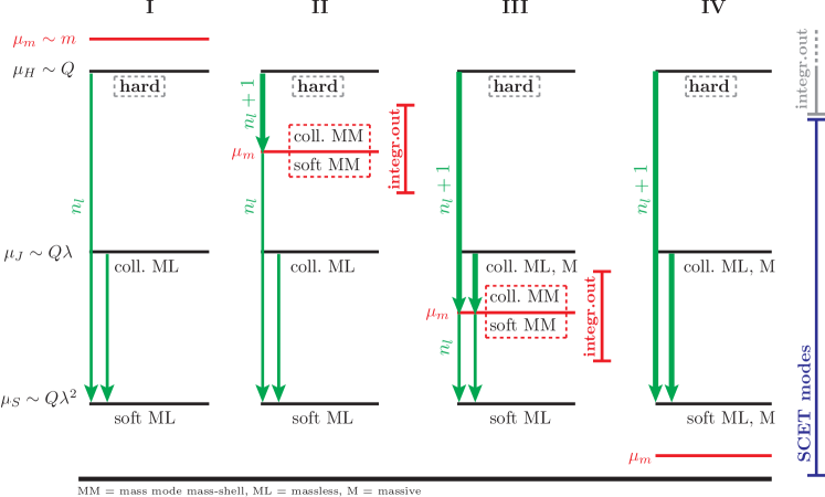
Note that some of the notation, the formulation of the factorization theorems and the organization of the RG evolution we use for the presentation of the results in this section are related to the choice that the final renormalization scale μ𝜇\mu is set to be equal to the soft scale, μ=μS𝜇subscript𝜇𝑆\mu=\mu_{S} such that the soft evolution factor US(,μS,μS)=δ()subscript𝑈𝑆subscript𝜇𝑆subscript𝜇𝑆𝛿U_{S}(\ell,\mu_{S},\mu_{S})=\delta(\ell) and can be dropped. Thus only the current and jet function RG evolution factors UCsubscript𝑈𝐶U_{C} and UJsubscript𝑈𝐽U_{J}, respectively, appear. The RG pattern of this “top-down” approach together with a graphical display of how the collinear and soft massive modes give contributions is illustrated in Fig. 4. Clearly, any other choice for μ𝜇\mu is possible and can significantly affect the form as well as the interpretation of the various components of the factorization theorems in the different scenarios. Since the number of possibilities in connection with the different scenarios and the choices for μ𝜇\mu in the factorization theorems proliferates strongly, we postpone a more general discussion to Sec. V, where we focus more on the RG properties of the hard coefficient and the jet and soft functions rather than on the full factorization theorem. This allows us to streamline the discussion significantly and to generalize our results to other processes.
Refer to caption
Figure 4: The different scenarios depending on the hierarchy between the mass scale μmsubscript𝜇𝑚\mu_{m} and the hard, jet and ultrasoft scales. MM indicates mass-shell scaling, ML the massless one. With M we denote modes that have a mass m𝑚m but scale as their massless counterparts. The renormalization group evolution is also shown in the top-down evolution from the hard scale μHsubscript𝜇𝐻\mu_{H} down to μ=μS𝜇subscript𝜇𝑆\mu=\mu_{S}. When the mass scale is crossed the mass-shell fluctuations are integrated out (dashed box). This leads to a matching condition and to a change in the evolution factor.

III.1 Scenario I: m>Q>Qλ>Qλ2𝑚𝑄𝑄𝜆𝑄superscript𝜆2m>Q>Q\lambda>Q\lambda^{2}

When the mass m𝑚m is larger than the hard scale Q𝑄Q the massive quark is not described in SCET, but integrated out when SCET is matched to QCD. The factorization theorem is the one for nlsubscript𝑛𝑙n_{l} massless fermions in analogy to Eq. (2) up to the hard current matching coefficient which acquires an additional contribution due to the heavy quark,

1σ0dσdτ=Q|C(nl)(Q,m,μH)|2|UC(nl)(Q,μH,μS)|21subscript𝜎0d𝜎d𝜏𝑄superscriptsuperscript𝐶subscript𝑛𝑙𝑄𝑚subscript𝜇𝐻2superscriptsubscriptsuperscript𝑈subscript𝑛𝑙𝐶𝑄subscript𝜇𝐻subscript𝜇𝑆2\displaystyle\frac{1}{\sigma_{0}}\frac{\mathrm{d}\sigma}{\mathrm{d}\tau}=Q\,\big{|}C^{(n_{l})}(Q,m,\mu_{H})\big{|}^{2}\,\big{|}U^{(n_{l})}_{C}(Q,\mu_{H},\mu_{S})\big{|}^{2}
×dsdsJ(nl)(s,μJ)UJ(nl)(ss,μS,μJ)\displaystyle\times\int\!\mathrm{d}s\!\int\!\mathrm{d}s^{\prime}\,J^{(n_{l})}(s^{\prime},\mu_{J})\,U^{(n_{l})}_{J}(s-s^{\prime},\mu_{S},\mu_{J})
×S(nl)(QτsQ,μS),absentsuperscript𝑆subscript𝑛𝑙𝑄𝜏𝑠𝑄subscript𝜇𝑆\displaystyle\times S^{(n_{l})}\Big{(}Q\,\tau-\frac{s}{Q},\mu_{S}\Big{)}\,, (27)

where

C(nl)(Q,m,μ)=C(nl)(Q,μ)+FQCD(nl,2)(Q,m).superscript𝐶subscript𝑛𝑙𝑄𝑚𝜇superscript𝐶subscript𝑛𝑙𝑄𝜇subscriptsuperscript𝐹subscript𝑛𝑙2QCD𝑄𝑚\displaystyle C^{(n_{l})}(Q,m,\mu)=C^{(n_{l})}(Q,\mu)+F^{(n_{l},2)}_{\rm QCD}(Q,m)\,. (28)

The term FQCD(nl,2)subscriptsuperscript𝐹subscript𝑛𝑙2QCDF^{(n_{l},2)}_{\rm QCD} represents the massive quark bubble contribution to the QCD current form factor, see the diagram in Fig. 1(a). Scenario I is designed to show manifest decoupling in the infinite mass limit, i.e.

C(nl)(Q,m,μ)C(nl)(Q,μ).\displaystyle C^{(n_{l})}(Q,m\rightarrow\infty,\mu)\rightarrow C^{(n_{l})}(Q,\mu)\,. (29)

This is achieved in FQCD(nl,2)subscriptsuperscript𝐹subscript𝑛𝑙2QCDF^{(n_{l},2)}_{\rm QCD} by two ingredients. First, the on-shell condition for the external quarks is related to a subtraction of the form factor at Q2=0superscript𝑄20Q^{2}=0 concerning the virtual secondary massive quark effects. Second, the massive quark bubble contribution to the strong coupling constant is renormalized in the on-shell scheme rather than in MS¯¯MS\overline{\rm MS}. 777The massless quark bubble contributions are still renormalized in the MS¯¯MS\overline{\rm MS} scheme as usual. So the massive quark is not an active dynamic flavor and does not contribute to the RG evolution of the strong coupling. One can derive the expression by first calculating the corresponding one-loop diagram with a massive gauge boson in Fig. 2(a) and then using the subtracted form of the dispersion relation according to Fig. 3. This yields 888Throughout the paper we suppress the dependence on the renormalization scale μ𝜇\mu in the arguments of terms which are just implicitly depending on the renormalization scale through αssubscript𝛼𝑠\alpha_{s} and the mass m𝑚m. (αs(nl)=αs(nl)(μ)superscriptsubscript𝛼𝑠subscript𝑛𝑙superscriptsubscript𝛼𝑠subscript𝑛𝑙𝜇\alpha_{s}^{(n_{l})}=\alpha_{s}^{(n_{l})}(\mu))

FQCD(nl,2)(Q,m)subscriptsuperscript𝐹subscript𝑛𝑙2QCD𝑄𝑚\displaystyle F^{(n_{l},2)}_{\rm QCD}(Q,m) FQCD(2,OS)(Q,m)absentsubscriptsuperscript𝐹2OSQCD𝑄𝑚\displaystyle\equiv F^{(2,\rm OS)}_{\rm QCD}(Q,m)
=(αs(nl))2CFTF16π2fQCD(2)(m/Q),absentsuperscriptsuperscriptsubscript𝛼𝑠subscript𝑛𝑙2subscript𝐶𝐹subscript𝑇𝐹16superscript𝜋2subscriptsuperscript𝑓2QCD𝑚𝑄\displaystyle=\frac{\big{(}\alpha_{s}^{(n_{l})}\big{)}^{2}C_{\!F}T_{F}}{16\pi^{2}}f^{(2)}_{\rm QCD}(m/Q)\,, (30)

where the function fQCD(2)(x)subscriptsuperscript𝑓2QCD𝑥f^{(2)}_{\rm QCD}(x) is given by Kniehl1990 ; Hoang:1995fr

fQCD(2)(x)=(469r3+103r)[Li2(r1r+1)Li2(r+1r1)]subscriptsuperscript𝑓2QCD𝑥469superscript𝑟3103𝑟delimited-[]subscriptLi2𝑟1𝑟1subscriptLi2𝑟1𝑟1\displaystyle\!\!f^{(2)}_{\rm QCD}(x)=\Big{(}\frac{46}{9}\,r^{3}+\frac{10}{3}\,r\Big{)}\!\bigg{[}\textrm{Li}_{2}\bigg{(}\frac{r-1}{r+1}\bigg{)}-\textrm{Li}_{2}\bigg{(}\frac{r+1}{r-1}\bigg{)}\bigg{]}
+(r4+2r2+53)[Li3(r1r+1)+Li3(r+1r1)2ζ3]superscript𝑟42superscript𝑟253delimited-[]subscriptLi3𝑟1𝑟1subscriptLi3𝑟1𝑟12subscript𝜁3\displaystyle\!\!+\Big{(}\!-r^{4}+2\,r^{2}+\frac{5}{3}\Big{)}\!\bigg{[}\textrm{Li}_{3}\bigg{(}\frac{r-1}{r+1}\bigg{)}+\textrm{Li}_{3}\bigg{(}\frac{r+1}{r-1}\bigg{)}-2\,\zeta_{3}\bigg{]}
+(1109r2+20027)ln(1r24)+2389r2+121381,1109superscript𝑟220027ln1superscript𝑟242389superscript𝑟2121381\displaystyle\!\!+\Big{(}\frac{110}{9}\,r^{2}+\frac{200}{27}\Big{)}\textrm{ln}\Big{(}\frac{1-r^{2}}{4}\Big{)}+\frac{238}{9}\,r^{2}+\frac{1213}{81}\,, (31)

and we have defined

x2=m2Q2+i 0,r=1+4x2.formulae-sequencesuperscript𝑥2superscript𝑚2superscript𝑄2𝑖 0𝑟14superscript𝑥2\displaystyle x^{2}=\frac{m^{2}}{Q^{2}+i\,0}\,,\quad r=\sqrt{1+4\,x^{2}}\,. (32)

In the limit m𝑚m\to\infty the massive quark decouples indeed, i.e. fQCD(2)(x)0subscriptsuperscript𝑓2QCD𝑥0f^{(2)}_{\rm QCD}(x)\rightarrow 0 for x𝑥x\to\infty. For light fermions, i.e. x0𝑥0x\rightarrow 0, we find

fQCD(2)(x)|x0=49ln3(x2)+389ln2(x2)evaluated-atsubscriptsuperscript𝑓2QCD𝑥𝑥049superscriptln3superscript𝑥2389superscriptln2superscript𝑥2\displaystyle\left.f^{(2)}_{\rm QCD}(x)\right|_{x\rightarrow 0}=\frac{4}{9}\,\textrm{ln}^{3}{(-x^{2})}+\frac{38}{9}\,\textrm{ln}^{2}{(-x^{2})} (33)
+(53027+4π29)ln(x2)+335581+38π227163ζ3,530274superscript𝜋29lnsuperscript𝑥233558138superscript𝜋227163subscript𝜁3\displaystyle+\bigg{(}\frac{530}{27}+\frac{4\pi^{2}}{9}\bigg{)}\textrm{ln}{(-x^{2})}+\frac{3355}{81}+\frac{38\pi^{2}}{27}-\frac{16}{3}\,\zeta_{3}\,,

with subleading corrections going as 𝒪(x2)𝒪superscript𝑥2\mathcal{O}(x^{2}). Eq. (33) does not bear any similarity to the massless result of Eq. (4) and further exhibits large unresummed mass logarithms. Thus the QCD result of Eq. (III.1) is not suitable for taking the massless limit. This is because Eq. (III.1) still contains mass mode on-shell contributions which must be subtracted prior to taking the limit mQmuch-less-than𝑚𝑄m\ll Q. This procedure is described in scenario II.

III.2 Scenario II: Q>m>Qλ>Qλ2𝑄𝑚𝑄𝜆𝑄superscript𝜆2Q>m>Q\lambda>Q\lambda^{2}

The mass m𝑚m is below the hard scale, but still above the jet and the soft scales. It is our aim (i) to resum the mass logarithms in Eq. (33) and (ii) to determine the hard current matching coefficient such that it contains no mass-singularities and in particular approaches the massless limit for m0𝑚0m\rightarrow 0. The collinear and soft mass modes are included into the SCET setup, so that they render the hard coefficient IR safe by subtracting the mass-shell contributions in the matching procedure. They contribute as dynamic degrees of freedom to the RG evolution above m𝑚m. In the RG evolution of the current from the hard to the jet scale the mass-shell fluctuations are finally integrated out at the scale m𝑚m. The mass mode effects are purely virtual because the jet scale Qλ𝑄𝜆Q\lambda, the typical invariant mass for real collinear particle radiation is below m𝑚m. Therefore, the jet and soft functions as well as their RG evolution factors towards scales smaller than m𝑚m coincide with the ones for nlsubscript𝑛𝑙n_{l} massless quarks. The factorization theorem reads

1σ0dσdτ=Q|C(nl+1)(Q,m,μH)|2|UC(nl+1)(Q,μH,μm)|21subscript𝜎0d𝜎d𝜏𝑄superscriptsuperscript𝐶subscript𝑛𝑙1𝑄𝑚subscript𝜇𝐻2superscriptsubscriptsuperscript𝑈subscript𝑛𝑙1𝐶𝑄subscript𝜇𝐻subscript𝜇𝑚2\displaystyle\frac{1}{\sigma_{0}}\frac{\mathrm{d}\sigma}{\mathrm{d}\tau}=Q\,\big{|}C^{(n_{l}+1)}(Q,m,\mu_{H})\big{|}^{2}\,\big{|}U^{(n_{l}+1)}_{C}(Q,\mu_{H},\mu_{m})\big{|}^{2}
×|C(Q,m,μm)|2|UC(nl)(Q,μm,μS)|2absentsuperscriptsubscript𝐶𝑄𝑚subscript𝜇𝑚2superscriptsubscriptsuperscript𝑈subscript𝑛𝑙𝐶𝑄subscript𝜇𝑚subscript𝜇𝑆2\displaystyle\times\big{|}{\mathcal{M}_{C}(Q,m,\mu_{m})}\big{|}^{2}\,\big{|}U^{(n_{l})}_{C}(Q,\mu_{m},\mu_{S})\big{|}^{2}
×dsdsJ(nl)(s,μJ)UJ(nl)(ss,μS,μJ)\displaystyle\times\int\!\mathrm{d}s\!\int\!\mathrm{d}s^{\prime}\,J^{(n_{l})}(s^{\prime},\mu_{J})\,U^{(n_{l})}_{J}(s-s^{\prime},\mu_{S},\mu_{J})
×S(nl)(QτsQ,μS).absentsuperscript𝑆subscript𝑛𝑙𝑄𝜏𝑠𝑄subscript𝜇𝑆\displaystyle\times S^{(n_{l})}\Big{(}Q\,\tau-\frac{s}{Q},\mu_{S}\Big{)}\,. (34)

Compared to C(nl)(Q,m,μH)superscript𝐶subscript𝑛𝑙𝑄𝑚subscript𝜇𝐻C^{(n_{l})}(Q,m,\mu_{H}) in Eq. (28) the hard current coefficient C(nl+1)(Q,m,μH)superscript𝐶subscript𝑛𝑙1𝑄𝑚subscript𝜇𝐻C^{(n_{l}+1)}(Q,m,\mu_{H}) acquires a subtractive contribution arising from the non-vanishing SCET diagrams involving virtual collinear and soft mass modes and contributions related to the use of the MS¯¯MS\overline{\rm MS} renormalization prescription for the strong coupling rather than the OS one concerning the massive quark bubble. The latter correction means that the massive quark now contributes to the RG evolution, and that we employ αs(nl+1)superscriptsubscript𝛼𝑠subscript𝑛𝑙1\alpha_{s}^{(n_{l}+1)}. The result for C(nl+1)(Q,m,μ)superscript𝐶subscript𝑛𝑙1𝑄𝑚𝜇C^{(n_{l}+1)}(Q,m,\mu) reads

C(nl+1)(Q,m,μ)=C(nl+1)(Q,μ)+δF(nl+1,2)(Q,m).superscript𝐶subscript𝑛𝑙1𝑄𝑚𝜇superscript𝐶subscript𝑛𝑙1𝑄𝜇𝛿superscript𝐹subscript𝑛𝑙12𝑄𝑚\displaystyle C^{(n_{l}+1)}(Q,m,\mu)=C^{(n_{l}+1)}(Q,\mu)+\delta F^{(n_{l}+1,2)}(Q,m)\,. (35)

The term δF(nl+1,2)𝛿superscript𝐹subscript𝑛𝑙12\delta F^{(n_{l}+1,2)} represents the corrections due to the non-vanishing mass of the heavy quark and can be written as (αs(nl+1)=αs(nl+1)(μ)superscriptsubscript𝛼𝑠subscript𝑛𝑙1superscriptsubscript𝛼𝑠subscript𝑛𝑙1𝜇\alpha_{s}^{(n_{l}+1)}=\alpha_{s}^{(n_{l}+1)}(\mu))

δF(nl+1,2)(Q,m)=(αs(nl+1))2CFTF16π2𝛿superscript𝐹subscript𝑛𝑙12𝑄𝑚superscriptsuperscriptsubscript𝛼𝑠subscript𝑛𝑙12subscript𝐶𝐹subscript𝑇𝐹16superscript𝜋2\displaystyle\delta F^{(n_{l}+1,2)}(Q,m)=\frac{\big{(}\alpha_{s}^{(n_{l}+1)}\big{)}^{2}C_{\!F}T_{F}}{16\pi^{2}}
×[fQCD(2)(m/Q)fQCD(2)(m/Q)|m0],absentdelimited-[]subscriptsuperscript𝑓2QCD𝑚𝑄evaluated-atsubscriptsuperscript𝑓2QCD𝑚𝑄𝑚0\displaystyle\times\left[f^{(2)}_{\rm QCD}(m/Q)-\left.f^{(2)}_{\rm QCD}(m/Q)\right|_{m\rightarrow 0}\right]\,, (36)

which can be read off Eqs. (III.1) and (33). All calculational steps are explained in detail in Sec. IV.2. One can check explicitly that all of the IR divergent mass-shell contributions are removed and that the massless limit for Eq. (35) is recovered for m0𝑚0m\rightarrow 0, i.e. δF(nl+1,2)(Q,m)m00superscript𝑚0𝛿superscript𝐹subscript𝑛𝑙12𝑄𝑚0\delta F^{(n_{l}+1,2)}(Q,m)\stackrel{{\scriptstyle m\rightarrow 0}}{{\longrightarrow}}0. We note that in the results of the collinear, the soft and the soft mass mode bin contributions there are rapidity divergences that cancel in the sum of all terms. We stress, however, that for μQsimilar-to𝜇𝑄\mu\sim Q no large (rapidity) logarithm remains in the hard current matching.

Note that the UV divergences of the bare SCET form factor are insensitive to the non-vanishing quark mass, such that we get in total the UV divergences from Eq. (5) for nf=nl+1subscript𝑛𝑓subscript𝑛𝑙1n_{\!f}=n_{l}+1. This argument does not rely on a specific order in αssubscript𝛼𝑠\alpha_{s}, so the evolution factor UC(nl+1)subscriptsuperscript𝑈subscript𝑛𝑙1𝐶U^{(n_{l}+1)}_{C} obeys the RG equation

μddμUC(nl+1)(Q,μH,μ)𝜇dd𝜇subscriptsuperscript𝑈subscript𝑛𝑙1𝐶𝑄subscript𝜇𝐻𝜇\displaystyle\mu\,\frac{\mathrm{d}}{\mathrm{d}\mu}\,U^{(n_{l}+1)}_{C}(Q,\mu_{H},\mu)
=γC(nl+1)(Q,μ)UC(nl+1)(Q,μH,μ)absentsubscriptsuperscript𝛾subscript𝑛𝑙1𝐶𝑄𝜇subscriptsuperscript𝑈subscript𝑛𝑙1𝐶𝑄subscript𝜇𝐻𝜇\displaystyle=\gamma^{(n_{l}+1)}_{C}(Q,\mu)\,U^{(n_{l}+1)}_{C}(Q,\mu_{H},\mu)\, (37)

to all orders in perturbative QCD for scales μ>μm𝜇subscript𝜇𝑚\mu>\mu_{m}.

At the scale μmsubscript𝜇𝑚\mu_{m} the mass-shell fluctuations of the collinear and soft mass modes are integrated out. This leads to the current mass mode matching coefficient C(Q,m,μm)subscript𝐶𝑄𝑚subscript𝜇𝑚\mathcal{M}_{C}(Q,m,\mu_{m}), which is the analogue of the well-known matching correction between the strong coupling schemes with nl+1subscript𝑛𝑙1n_{l}+1 and nlsubscript𝑛𝑙n_{l} running dynamic flavors, αs(nl+1)superscriptsubscript𝛼𝑠subscript𝑛𝑙1\alpha_{s}^{(n_{l}+1)} and αs(nl)superscriptsubscript𝛼𝑠subscript𝑛𝑙\alpha_{s}^{(n_{l})} respectively. The result reads (αsln(m2/Q2)𝒪(1)similar-tosubscript𝛼𝑠lnsuperscript𝑚2superscript𝑄2𝒪1\alpha_{s}\,\textrm{ln}(m^{2}/Q^{2})\sim\mathcal{O}(1))

C(Q,m,μH,μm)=1+[(αs(nl+1))2CFTF(4π)2ln(μH2μm2){43Lm2409Lm11227}]𝒪(αs)subscript𝐶𝑄𝑚subscript𝜇𝐻subscript𝜇𝑚1subscriptdelimited-[]superscriptsuperscriptsubscript𝛼𝑠subscript𝑛𝑙12subscript𝐶𝐹subscript𝑇𝐹superscript4𝜋2lnsuperscriptsubscript𝜇𝐻2superscriptsubscript𝜇𝑚243superscriptsubscript𝐿𝑚2409subscript𝐿𝑚11227𝒪subscript𝛼𝑠\displaystyle\mathcal{M}_{C}(Q,m,\mu_{H},\mu_{m})=1+\left[\frac{\big{(}\alpha_{s}^{(n_{l}+1)}\big{)}^{2}C_{\!F}T_{F}}{(4\pi)^{2}}\textrm{ln}\left(\frac{\mu_{H}^{2}}{\mu_{m}^{2}}\right)\left\{-\frac{4}{3}\,L_{m}^{2}-\frac{40}{9}\,L_{m}-\frac{112}{27}\right\}\right]_{\mathcal{O}(\alpha_{s})}
+[(αs(nl+1))2CFTF(4π)2{49Lm3+389Lm2+(24227+2π23)Lmln(Q2μH2){43Lm2+409Lm+11227}+87554+5π29529ζ3}\displaystyle+\left[\frac{\big{(}\alpha_{s}^{(n_{l}+1)}\big{)}^{2}C_{\!F}T_{F}}{(4\pi)^{2}}\left\{\frac{4}{9}\,L_{m}^{3}+\frac{38}{9}\,L_{m}^{2}+\left(\frac{242}{27}+\frac{2\pi^{2}}{3}\right)\!L_{m}-\textrm{ln}\bigg{(}\!\!-\frac{Q^{2}}{\mu_{H}^{2}}\bigg{)}\!\left\{\frac{4}{3}\,L_{m}^{2}+\frac{40}{9}\,L_{m}+\frac{112}{27}\right\}+\frac{875}{54}+\frac{5\pi^{2}}{9}-\frac{52}{9}\,\zeta_{3}\right\}\right.
+(αs(nl+1))3CFTF(4π)3ln(μH2μm2){Lm3[8827CA6427TF3227TFnl]+Lm2[(929+89π2)CA+12CF16027TF]\displaystyle+\frac{\big{(}\alpha_{s}^{(n_{l}+1)}\big{)}^{3}C_{\!F}T_{F}}{(4\pi)^{3}}\,\textrm{ln}\bigg{(}\frac{\mu_{H}^{2}}{\mu_{m}^{2}}\bigg{)}\!\left\{L_{m}^{3}\!\left[\frac{88}{27}\,C_{\!A}-\frac{64}{27}\,T_{F}-\frac{32}{27}\,T_{F}n_{l}\right]+L_{m}^{2}\!\left[\left(-\frac{92}{9}+\frac{8}{9}\pi^{2}\right)\!C_{\!A}+12\,C_{\!F}-\frac{160}{27}\,T_{F}\right]\right.
+Lm[(62081+80π2271123ζ3)CA+(43+32ζ3)CF108881TFnl99281TF]3C,+CFTF}\displaystyle+\left.L_{m}\left[\left(-\frac{620}{81}+\frac{80\pi^{2}}{27}-\frac{112}{3}\,\zeta_{3}\right)\!C_{\!A}+\left(-\frac{4}{3}+32\,\zeta_{3}\right)\!C_{\!F}-\frac{1088}{81}\,T_{F}n_{l}-\frac{992}{81}\,T_{F}\right]-\frac{\mathcal{M}_{3}^{C,+}}{C_{\!F}T_{F}}\right\}
+(αs(nl+1))4CF2TF2(4π)4ln2(μH2μm2){89Lm4+16027Lm3+41627Lm2+4480243Lm+6272729}]𝒪(αs2),\displaystyle+\left.\frac{\big{(}\alpha_{s}^{(n_{l}+1)}\big{)}^{4}C_{\!F}^{2}T_{F}^{2}}{(4\pi)^{4}}\,\textrm{ln}^{2}\bigg{(}\frac{\mu_{H}^{2}}{\mu_{m}^{2}}\bigg{)}\!\left\{\frac{8}{9}\,L_{m}^{4}+\frac{160}{27}\,L_{m}^{3}+\frac{416}{27}L_{m}^{2}+\frac{4480}{243}\,L_{m}+\frac{6272}{729}\right\}\right]_{\mathcal{O}(\alpha_{s}^{2})}\,, (38)

where Q2=Q2+i0superscript𝑄2superscript𝑄2𝑖0Q^{2}=Q^{2}+i0, Lmln(m2/μm2)subscript𝐿𝑚lnsuperscript𝑚2superscriptsubscript𝜇𝑚2L_{m}\equiv\textrm{ln}{\left(m^{2}/\mu_{m}^{2}\right)} and αs(nl+1)=αs(nl+1)(μm)superscriptsubscript𝛼𝑠subscript𝑛𝑙1superscriptsubscript𝛼𝑠subscript𝑛𝑙1subscript𝜇𝑚\alpha_{s}^{(n_{l}+1)}=\alpha_{s}^{(n_{l}+1)}(\mu_{m}). The quark mass mm¯(μm)𝑚¯𝑚subscript𝜇𝑚m\equiv\overline{m}(\mu_{m}) is given in the MS¯¯MS\overline{\rm MS} scheme. We see that the result contains large logarithms ln(μm2/μH2)lnsuperscriptsubscript𝜇𝑚2superscriptsubscript𝜇𝐻2\textrm{ln}(\mu_{m}^{2}/\mu_{H}^{2}), which are not summed by the RG μ𝜇\mu-evolution of the current. These logarithms are related to rapidity singularities that arise in the overlap region between the collinear and soft mass modes, all having invariant masses of order m2superscript𝑚2m^{2}. Analogous logarithmic terms were also found for the 𝒪(αs)𝒪subscript𝛼𝑠\mathcal{O}(\alpha_{s}) massive gluon results discussed in Ref. Gritschacher:2013pha . There are several approaches to resum these rapidity logarithms Becher:2011dz ; Chiu:2012ir ; Chiu:2011qc , but the outcome is just a simple exponentiation which yields the term at 𝒪(αs4ln2(m2/Q2))𝒪superscriptsubscript𝛼𝑠4superscriptln2superscript𝑚2superscript𝑄2\mathcal{O}(\alpha_{s}^{4}\,\textrm{ln}^{2}(m^{2}/Q^{2})) in Eq. (38). We refer to Ref. Hoang:2015vua for a calculation of the anomalous dimension in rapidity space. We note that through the rapidity RG evolution Csubscript𝐶\mathcal{M}_{C} depends at each order on two rapidity scales. For simplicity we correlate them with the two invariant mass scales μHsubscript𝜇𝐻\mu_{H} and μmsubscript𝜇𝑚\mu_{m}. We stress, however, that the dependence of Csubscript𝐶\mathcal{M}_{C} on the hard matching scale μHsubscript𝜇𝐻\mu_{H} is actually spurious and cancels in an expansion at fixed-order in αssubscript𝛼𝑠\alpha_{s}. The existence of the large logarithms has the important consequence that the 𝒪(αs2ln(m2/Q2))𝒪superscriptsubscript𝛼𝑠2lnsuperscript𝑚2superscript𝑄2\mathcal{O}(\alpha_{s}^{2}\,\textrm{ln}(m^{2}/Q^{2})) corrections in Eq. (38) enter at the same order as the 𝒪(αs)𝒪subscript𝛼𝑠\mathcal{O}(\alpha_{s}) fixed-order corrections based on the counting αsln(m2/Q2)𝒪(1)similar-tosubscript𝛼𝑠lnsuperscript𝑚2superscript𝑄2𝒪1\alpha_{s}\,\textrm{ln}(m^{2}/Q^{2})\sim\mathcal{O}(1) and thus contribute already at N2LL order where one-loop fixed-order corrections to the hard coefficient and the jet and the soft functions are accounted for. At N3LL order we therefore need the terms at 𝒪(αs3ln(m2/Q2))𝒪superscriptsubscript𝛼𝑠3lnsuperscript𝑚2superscript𝑄2\mathcal{O}(\alpha_{s}^{3}\,\textrm{ln}(m^{2}/Q^{2})) and 𝒪(αs4ln2(m2/Q2))𝒪superscriptsubscript𝛼𝑠4superscriptln2superscript𝑚2superscript𝑄2\mathcal{O}(\alpha_{s}^{4}\,\textrm{ln}^{2}(m^{2}/Q^{2})). 999In the primed counting one might still need to distinguish between terms enhanced by rapidity logarithms (and related to terms summed by the rapidity RGE) and the remaining terms in the series for the mass mode threshold factors. We have indicated this counting by using the subscripts ``𝒪(αs)"``𝒪subscript𝛼𝑠"``\mathcal{O}(\alpha_{s})" and ``𝒪(αs2)"``𝒪superscriptsubscript𝛼𝑠2"``\mathcal{O}(\alpha_{s}^{2})" in the result of Eq. (38). From the 𝒪(αs3ln(m2/Q2))𝒪superscriptsubscript𝛼𝑠3lnsuperscript𝑚2superscript𝑄2\mathcal{O}(\alpha_{s}^{3}\,\textrm{ln}(m^{2}/Q^{2})) terms the contributions explicitly depending on μmsubscript𝜇𝑚\mu_{m} can be inferred using the μmsubscript𝜇𝑚\mu_{m}-independence of the factorization theorem and the explicit form of the current evolution factors UC(nl+1)superscriptsubscript𝑈𝐶subscript𝑛𝑙1U_{C}^{(n_{l}+1)} and UC(nl)superscriptsubscript𝑈𝐶subscript𝑛𝑙U_{C}^{(n_{l})}. In Eq. (38) the full form of the 𝒪(αs3ln(m2/Q2))𝒪superscriptsubscript𝛼𝑠3lnsuperscript𝑚2superscript𝑄2\mathcal{O}(\alpha_{s}^{3}\,\textrm{ln}(m^{2}/Q^{2})) term is displayed with the constant 3C,+superscriptsubscript3𝐶\mathcal{M}_{3}^{C,+} which cannot be determined from RG arguments. This constant corresponds to a rapidity logarithm that is physically unrelated to logarithms of μmsubscript𝜇𝑚\mu_{m}. Details of these computations can be found in Sec. V.1.

III.3 Scenario III: Q>Qλ>m>Qλ2𝑄𝑄𝜆𝑚𝑄superscript𝜆2Q>Q\lambda>m>Q\lambda^{2}

The mass is between the jet and the soft scales. The current evolution is the same as the one in scenario II and the soft function still includes only the effects of the nlsubscript𝑛𝑙n_{l} massless quarks. Since the massless as well as the massive collinear modes both can now fluctuate in the collinear sector the difference to scenario II concerns the jet function, where additional massive real and virtual contributions arise. The setup is constructed such that it (i) sums all mass logarithms that arise in the evolution of the jet function and (ii) ensures that the jet function approaches the known massless result for nl+1subscript𝑛𝑙1n_{l}+1 flavors in the limit m0𝑚0m\rightarrow 0. In analogy to the current, the RG evolution of the jet function is performed with nl+1subscript𝑛𝑙1n_{l}+1 flavors above the mass threshold. Collinear mass-shell fluctuations are integrated out at the mass scale yielding a collinear mass mode matching coefficient Jsubscript𝐽\mathcal{M}_{J}, and the evolution continues with nlsubscript𝑛𝑙n_{l} light quarks down to the soft scale. Overall, the factorization theorem in this scenario has the form

1σ0dσdτ=Q|C(nl+1)(Q,m,μH)|2|UC(nl+1)(Q,μH,μm)|21subscript𝜎0d𝜎d𝜏𝑄superscriptsuperscript𝐶subscript𝑛𝑙1𝑄𝑚subscript𝜇𝐻2superscriptsubscriptsuperscript𝑈subscript𝑛𝑙1𝐶𝑄subscript𝜇𝐻subscript𝜇𝑚2\displaystyle\frac{1}{\sigma_{0}}\frac{\mathrm{d}\sigma}{\mathrm{d}\tau}=Q\,\big{|}C^{(n_{l}+1)}(Q,m,\mu_{H})\big{|}^{2}\,\big{|}U^{(n_{l}+1)}_{C}(Q,\mu_{H},\mu_{m})\big{|}^{2}
×|C(Q,m,μm)|2|UC(nl)(Q,μm,μS)|2absentsuperscriptsubscript𝐶𝑄𝑚subscript𝜇𝑚2superscriptsubscriptsuperscript𝑈subscript𝑛𝑙𝐶𝑄subscript𝜇𝑚subscript𝜇𝑆2\displaystyle\times\big{|}{\mathcal{M}_{C}(Q,m,\mu_{m})}\big{|}^{2}\,\big{|}U^{(n_{l})}_{C}(Q,\mu_{m},\mu_{S})\big{|}^{2}
×dsdsds′′ds′′′J(nl+1)(s′′′,m,μJ)\displaystyle\times\int\!\mathrm{d}s\!\int\!\mathrm{d}s^{\prime}\!\int\!\mathrm{d}s^{\prime\prime}\!\int\!\mathrm{d}s^{\prime\prime\prime}J^{(n_{l}+1)}(s^{\prime\prime\prime},m,\mu_{J})
×UJ(nl+1)(s′′s′′′,μm,μJ)J(ss′′,m,μm)absentsubscriptsuperscript𝑈subscript𝑛𝑙1𝐽superscript𝑠′′superscript𝑠′′′subscript𝜇𝑚subscript𝜇𝐽subscript𝐽superscript𝑠superscript𝑠′′𝑚subscript𝜇𝑚\displaystyle\times U^{(n_{l}+1)}_{J}(s^{\prime\prime}-s^{\prime\prime\prime},\mu_{m},\mu_{J})\,\mathcal{M}_{J}(s^{\prime}-s^{\prime\prime},m,\mu_{m})
×UJ(nl)(ss,μS,μm)S(nl)(QτsQ,μS),absentsubscriptsuperscript𝑈subscript𝑛𝑙𝐽𝑠superscript𝑠subscript𝜇𝑆subscript𝜇𝑚superscript𝑆subscript𝑛𝑙𝑄𝜏𝑠𝑄subscript𝜇𝑆\displaystyle\times U^{(n_{l})}_{J}(s-s^{\prime},\mu_{S},\mu_{m})\,S^{(n_{l})}\Big{(}Q\,\tau-\frac{s}{Q},\mu_{S}\Big{)}, (39)

where the matching coefficients C(nl+1)(Q,m,μH)superscript𝐶subscript𝑛𝑙1𝑄𝑚subscript𝜇𝐻C^{(n_{l}+1)}(Q,m,\mu_{H}) and C(Q,m,μm)subscript𝐶𝑄𝑚subscript𝜇𝑚\mathcal{M}_{C}(Q,m,\mu_{m}) are the same as in scenario II, see Eqs. (35) and (38). The jet function J(nl+1)(s,m,μ)superscript𝐽subscript𝑛𝑙1𝑠𝑚𝜇J^{(n_{l}+1)}(s,m,\mu) contains contributions related to virtual and real radiation of the massive secondary quarks and has the form

J(nl+1)(s,m,μ)=superscript𝐽subscript𝑛𝑙1𝑠𝑚𝜇absent\displaystyle J^{(n_{l}+1)}(s,m,\mu)= J(nl+1)(s,μ)+δJmdist(s,m,μ)superscript𝐽subscript𝑛𝑙1𝑠𝜇𝛿subscriptsuperscript𝐽dist𝑚𝑠𝑚𝜇\displaystyle\,J^{(n_{l}+1)}(s,\mu)+\delta J^{\rm{dist}}_{m}(s,m,\mu)
+δJmreal(s,m),𝛿subscriptsuperscript𝐽real𝑚𝑠𝑚\displaystyle+\delta J^{\rm{real}}_{m}(s,m)\,, (40)

where the two latter terms represent corrections due to the quark mass. The computation is described in Sec. IV.3. The expression for δJmdist(s,m,μ)𝛿subscriptsuperscript𝐽dist𝑚𝑠𝑚𝜇\delta J^{\rm{dist}}_{m}(s,m,\mu) contains only distributions and corresponds to collinear massive virtual corrections (including soft-bin subtractions) as well as terms related to the subtraction of the massless quark result contained in J(nl+1)(s,μ)superscript𝐽subscript𝑛𝑙1𝑠𝜇J^{(n_{l}+1)}(s,\mu) (see Eq. (II)). Its renormalized expression reads (s¯=s/μ2,αs(nl+1)=αs(nl+1)(μ)formulae-sequence¯𝑠𝑠superscript𝜇2superscriptsubscript𝛼𝑠subscript𝑛𝑙1superscriptsubscript𝛼𝑠subscript𝑛𝑙1𝜇\bar{s}=s/\mu^{2},\,\alpha_{s}^{(n_{l}+1)}=\alpha_{s}^{(n_{l}+1)}(\mu))

μ2δJmdist(s,m,μ)=(αs(nl+1))2CFTF16π2{[169Lm3\displaystyle\mu^{2}\delta J^{\rm{dist}}_{m}(s,m,\mu)=\frac{\big{(}\alpha_{s}^{(n_{l}+1)}\big{)}^{2}C_{\!F}T_{F}}{16\pi^{2}}\left\{\left[\frac{16}{9}\,L_{m}^{3}\right.\right.
+1169Lm2+(14362716π29)Lm+865081116π2271169superscriptsubscript𝐿𝑚214362716superscript𝜋29subscript𝐿𝑚865081116superscript𝜋227\displaystyle+\frac{116}{9}\,L_{m}^{2}+\left(\frac{1436}{27}-\frac{16\pi^{2}}{9}\right)\!L_{m}+\frac{8650}{81}-\frac{116\pi^{2}}{27}
643ζ3]δ(s¯)+(163Lm22329Lm143627\displaystyle-\left.\frac{64}{3}\,\zeta_{3}\right]\!\delta(\bar{s})+\left(-\frac{16}{3}L_{m}^{2}-\frac{232}{9}\,L_{m}-\frac{1436}{27}\right.
+16π29)[θ(s¯)s¯]++(323Lm+2329)[θ(s¯)lns¯s¯]+\displaystyle+\left.\frac{16\pi^{2}}{9}\right)\!\left[\frac{\theta(\bar{s})}{\bar{s}}\right]_{+}+\left(\frac{32}{3}\,L_{m}+\frac{232}{9}\right)\!\left[\frac{\theta(\bar{s})\textrm{ln}\,{\bar{s}}}{\bar{s}}\right]_{+}
163[θ(s¯)ln2s¯s¯]+}.\displaystyle-\left.\frac{16}{3}\!\left[\frac{\theta(\bar{s})\textrm{ln}^{2}\,{\bar{s}}}{\bar{s}}\right]_{+}\right\}\,. (41)

The term δJmreal(s,m)𝛿subscriptsuperscript𝐽real𝑚𝑠𝑚\delta J^{\rm{real}}_{m}(s,m) in Eq. (40) contributes only when the jet invariant mass is above the threshold 4m24superscript𝑚24m^{2} and thus corresponds to real production of the massive quarks. It is given by

μ2δJmreal(s,m)=(αs(nl+1))2CFTF16π21s¯θ(s4m2)superscript𝜇2𝛿subscriptsuperscript𝐽real𝑚𝑠𝑚superscriptsuperscriptsubscript𝛼𝑠subscript𝑛𝑙12subscript𝐶𝐹subscript𝑇𝐹16superscript𝜋21¯𝑠𝜃𝑠4superscript𝑚2\displaystyle\mu^{2}\delta J^{\rm{real}}_{m}(s,m)=\frac{\big{(}\alpha_{s}^{(n_{l}+1)}\big{)}^{2}C_{\!F}T_{F}}{16\pi^{2}}\frac{1}{\bar{s}}\,\theta(s-4m^{2})
×{643Li2(b1b+1)+323ln(1b24)ln(1b1+b)\displaystyle\times\bigg{\{}\!-\frac{64}{3}\,\textrm{Li}_{2}\bigg{(}\frac{b-1}{b+1}\bigg{)}+\frac{32}{3}\,\textrm{ln}{\left(\frac{1-b^{2}}{4}\right)}\textrm{ln}\bigg{(}\frac{1-b}{1+b}\bigg{)}
163ln2(1b1+b)+(b42b2+2419)ln(1b1+b)163superscriptln21𝑏1𝑏superscript𝑏42superscript𝑏22419ln1𝑏1𝑏\displaystyle-\frac{16}{3}\,\textrm{ln}^{2}\bigg{(}\frac{1-b}{1+b}\bigg{)}+\Big{(}b^{4}-2\,b^{2}+\frac{241}{9}\Big{)}\textrm{ln}\bigg{(}\frac{1-b}{1+b}\bigg{)}
1027b3+4829b16π29},\displaystyle-\frac{10}{27}\,b^{3}+\frac{482}{9}\,b-\frac{16\pi^{2}}{9}\bigg{\}}\,, (42)

with

b=14m2s.𝑏14superscript𝑚2𝑠\displaystyle\qquad b=\sqrt{1-\frac{4m^{2}}{s}}\,. (43)

Due to its physical character it is UV-finite and does not contain any explicit logarithmic μ𝜇\mu-dependence. Furthermore, δJmreal𝛿subscriptsuperscript𝐽real𝑚\delta J^{\rm{real}}_{m} and its first two derivatives in s𝑠s vanish at the threshold, so that no discontinuity arises due to real radiation. Note that the range in τ𝜏\tau where scenario III is employed may be chosen such that it fully includes the domain for collinear massive real radiation, namely τ4m2/Q2𝜏4superscript𝑚2superscript𝑄2\tau\geq 4m^{2}/Q^{2}, so that the threshold is properly accounted for through the analytic form of δJmreal(s,m,μm)𝛿subscriptsuperscript𝐽real𝑚𝑠𝑚subscript𝜇𝑚\delta J^{\rm{real}}_{m}(s,m,\mu_{m}). For m0𝑚0m\rightarrow 0 the jet function J(nl+1)(s,m,μ)superscript𝐽subscript𝑛𝑙1𝑠𝑚𝜇J^{(n_{l}+1)}(s,m,\mu) yields correctly the fully massless jet function at 𝒪(αs2)𝒪superscriptsubscript𝛼𝑠2\mathcal{O}(\alpha_{s}^{2}), i.e.

J(nl+1)(s,m,μ)m0J(nl+1)(s,μ).superscript𝑚0superscript𝐽subscript𝑛𝑙1𝑠𝑚𝜇superscript𝐽subscript𝑛𝑙1𝑠𝜇\displaystyle J^{(n_{l}+1)}(s,m,\mu)\stackrel{{\scriptstyle m\rightarrow 0}}{{\longrightarrow}}J^{(n_{l}+1)}(s,\mu)\,. (44)

We note that in the calculation of δJmdist𝛿superscriptsubscript𝐽𝑚dist\delta J_{m}^{\rm{dist}} rapidity divergences arise which cancel in the sum of the collinear diagrams and the corresponding soft-bin subtractions. We stress that for μ2ssimilar-tosuperscript𝜇2𝑠\mu^{2}\sim s all associated logarithms cancel completely in the sum of δJmreal𝛿superscriptsubscript𝐽𝑚real\delta J_{m}^{\rm{real}} and δJmdist𝛿subscriptsuperscript𝐽dist𝑚\delta J^{\rm{dist}}_{m}, so that no (large) rapidity logarithm remains in the jet function.

The UV divergences of the bare jet function Jbare(nl+1)(s,m,μ)subscriptsuperscript𝐽subscript𝑛𝑙1bare𝑠𝑚𝜇J^{(n_{l}+1)}_{\rm bare}(s,m,\mu) are mass independent and agree with the known massless ones for nl+1subscript𝑛𝑙1n_{l}+1 dynamic flavors. The 𝒪(αs2CFTF)𝒪superscriptsubscript𝛼𝑠2subscript𝐶𝐹subscript𝑇𝐹\mathcal{O}(\alpha_{s}^{2}C_{\!F}T_{F}) contributions to the jet function counterterm are the ones from Eq. (7) for nf=nl+1subscript𝑛𝑓subscript𝑛𝑙1n_{\!f}=n_{l}+1. This statement holds to any order in αssubscript𝛼𝑠\alpha_{s}, so that the jet function evolution factor UJ(nl+1)subscriptsuperscript𝑈subscript𝑛𝑙1𝐽U^{(n_{l}+1)}_{J} obeys

μddμUJ(nl+1)(s,μ,μJ)𝜇dd𝜇subscriptsuperscript𝑈subscript𝑛𝑙1𝐽𝑠𝜇subscript𝜇𝐽\displaystyle\mu\,\frac{\mathrm{d}}{\mathrm{d}\mu}\,U^{(n_{l}+1)}_{J}(s,\mu,\mu_{J})
=dsγJ(nl+1)(ss,μ)UJ(nl+1)(s,μ,μJ).absentdifferential-dsuperscript𝑠subscriptsuperscript𝛾subscript𝑛𝑙1𝐽𝑠superscript𝑠𝜇subscriptsuperscript𝑈subscript𝑛𝑙1𝐽superscript𝑠𝜇subscript𝜇𝐽\displaystyle=\int\!\mathrm{d}s^{\prime}\gamma^{(n_{l}+1)}_{J}(s-s^{\prime},\mu)\,U^{(n_{l}+1)}_{J}(s^{\prime},\mu,\mu_{J})\,. (45)

At the scale μmsubscript𝜇𝑚\mu_{m} the mass-shell fluctuations of the collinear mass modes are integrated out. These contributions are encoded in the jet mass mode matching coefficient J(s,m,μm)subscript𝐽𝑠𝑚subscript𝜇𝑚\mathcal{M}_{J}(s,m,\mu_{m}) and contain all virtual effects of the massive flavor such that for the scales μ<μm𝜇subscript𝜇𝑚\mu<\mu_{m} massive collinear effects decouple. The result up to 𝒪(αs2)𝒪superscriptsubscript𝛼𝑠2\mathcal{O}(\alpha_{s}^{2}) reads

μJ2J(2)(s,m,μJ,μm)=δ(s~)+[(αs(nl+1))2CFTF(4π)2δ(s~)ln(μJ2μm2)(163Lm2+1609Lm+44827)]𝒪(αs)superscriptsubscript𝜇𝐽2subscriptsuperscript2𝐽𝑠𝑚subscript𝜇𝐽subscript𝜇𝑚𝛿~𝑠subscriptdelimited-[]superscriptsuperscriptsubscript𝛼𝑠subscript𝑛𝑙12subscript𝐶𝐹subscript𝑇𝐹superscript4𝜋2𝛿~𝑠lnsuperscriptsubscript𝜇𝐽2superscriptsubscript𝜇𝑚2163superscriptsubscript𝐿𝑚21609subscript𝐿𝑚44827𝒪subscript𝛼𝑠\displaystyle\mu_{J}^{2}\,\mathcal{M}^{(2)}_{J}(s,m,\mu_{J},\mu_{m})=\delta(\tilde{s})+\left[\frac{\big{(}\alpha_{s}^{(n_{l}+1)}\big{)}^{2}C_{\!F}T_{F}}{(4\pi)^{2}}\,\delta(\tilde{s})\,\textrm{ln}\bigg{(}\frac{\mu_{J}^{2}}{\mu_{m}^{2}}\bigg{)}\!\!\left(\frac{16}{3}\,L_{m}^{2}+\frac{160}{9}\,L_{m}+\frac{448}{27}\right)\right]_{\mathcal{O}(\alpha_{s})}
+[(αs(nl+1))2CFTF(4π)2{[169Lm31169Lm2+(932278π29)Lm15312720π227+1609ζ3]δ(s~)\displaystyle+\Bigg{[}\frac{\big{(}\alpha_{s}^{(n_{l}+1)}\big{)}^{2}C_{\!F}T_{F}}{(4\pi)^{2}}\left\{\left[-\,\frac{16}{9}\,L_{m}^{3}-\frac{116}{9}\,L_{m}^{2}+\left(-\frac{932}{27}-\frac{8\pi^{2}}{9}\right)\!L_{m}-\frac{1531}{27}-\frac{20\pi^{2}}{27}+\frac{160}{9}\,\zeta_{3}\right]\!\delta(\tilde{s})\right.
+[163Lm2+1609Lm+44827][θ(s~)s~]+}+(αs(nl+1))3CFTF(4π)3δ(s~)ln(μJ2μm2){Lm3[35227CA+25627TF+12827TFnl]\displaystyle+\left.\left[\frac{16}{3}\,L_{m}^{2}+\frac{160}{9}\,L_{m}+\frac{448}{27}\right]\!\left[\frac{\theta(\tilde{s})}{\tilde{s}}\right]_{+}\right\}+\frac{\big{(}\alpha_{s}^{(n_{l}+1)}\big{)}^{3}C_{\!F}T_{F}}{(4\pi)^{3}}\,\delta(\tilde{s})\,\textrm{ln}\bigg{(}\frac{\mu_{J}^{2}}{\mu_{m}^{2}}\bigg{)}\!\left\{L_{m}^{3}\!\left[-\,\frac{352}{27}\,C_{\!A}+\frac{256}{27}\,T_{F}+\frac{128}{27}\,T_{F}n_{l}\right]\right.
+Lm2[(368932π29)CA48CF+64027TF]+Lm[(4483ζ3+248081320π227)CA+(163128ζ3)CF\displaystyle+L_{m}^{2}\!\left[\left(\frac{368}{9}-\frac{32\pi^{2}}{9}\right)\!C_{\!A}-48\,C_{\!F}+\frac{640}{27}\,T_{F}\right]+L_{m}\!\left[\left(\frac{448}{3}\,\zeta_{3}+\frac{2480}{81}-\frac{320\pi^{2}}{27}\right)\!C_{\!A}+\left(\frac{16}{3}-128\,\zeta_{3}\right)\!C_{\!F}\right.
+435281TFnl+396881TF]+3J,+CFTF}+(αs(nl+1))4CF2TF2(4π)4δ(s~)ln2(μJ2μm2)(1289Lm4+256027Lm3+665627Lm2\displaystyle\left.\left.+\frac{4352}{81}\,T_{F}\,n_{l}+\frac{3968}{81}\,T_{F}\right]+\frac{\mathcal{M}^{J,+}_{3}}{C_{\!F}T_{F}}\right\}+\frac{\big{(}\alpha_{s}^{(n_{l}+1)}\big{)}^{4}C_{\!F}^{2}T_{F}^{2}}{(4\pi)^{4}}\,\delta(\tilde{s})\,\textrm{ln}^{2}\bigg{(}\frac{\mu_{J}^{2}}{\mu_{m}^{2}}\bigg{)}\!\!\left(\frac{128}{9}\,L_{m}^{4}+\frac{2560}{27}\,L_{m}^{3}+\frac{6656}{27}\,L_{m}^{2}\right.
+71680243Lm+100352729)]𝒪(αs2),\displaystyle+\left.\frac{71680}{243}\,L_{m}+\frac{100352}{729}\right)\Bigg{]}_{\mathcal{O}(\alpha_{s}^{2})}\,, (46)

where s~s/μJ2~𝑠𝑠subscriptsuperscript𝜇2𝐽\tilde{s}\equiv s/\mu^{2}_{J}, Lmln(m2/μm2)subscript𝐿𝑚lnsuperscript𝑚2superscriptsubscript𝜇𝑚2L_{m}\equiv\textrm{ln}{\left(m^{2}/\mu_{m}^{2}\right)} and αs(nl+1)=αs(nl+1)(μm)superscriptsubscript𝛼𝑠subscript𝑛𝑙1superscriptsubscript𝛼𝑠subscript𝑛𝑙1subscript𝜇𝑚\alpha_{s}^{(n_{l}+1)}=\alpha_{s}^{(n_{l}+1)}(\mu_{m}). The quark mass m=m¯(μm)𝑚¯𝑚subscript𝜇𝑚m=\overline{m}(\mu_{m}) is given in the MS¯¯MS\overline{\rm MS} scheme. It is interesting to note that the result is a non-trivial distributive function of the jet invariant mass s𝑠s and thus differs substantially from the local mass mode matching coefficient of the current (see Eq. (38)) or the strong coupling which do not depend explicitly on any kinematic scale. As for the case of the current mass mode matching coefficient, Jsubscript𝐽\mathcal{M}_{J} contains large logarithms involving the ratio of the jet scale sμJsimilar-to𝑠subscript𝜇𝐽s\sim\mu_{J} and the mass scale mμmsimilar-to𝑚subscript𝜇𝑚m\sim\mu_{m} which are not summed by the RG μ𝜇\mu-evolution of the jet function. They are related to rapidity-type singularities that arise in the massive virtual corrections in the overlap region between the collinear mass mode contributions and their soft-bin subtractions. These logarithms exponentiate as in the case for the current mass mode matching coefficient. We note that, through the rapidity RG evolution, Jsubscript𝐽\mathcal{M}_{J} depends at each order on two rapidity scales, which we correlate to the jet and the mass scales μJsubscript𝜇𝐽\mu_{J} and μmsubscript𝜇𝑚\mu_{m}, respectively. We stress, however, that the dependence of Jsubscript𝐽\mathcal{M}_{J} on the jet scale μJsubscript𝜇𝐽\mu_{J} cancels in a fixed-order expansion. Using the counting αsln(m2/s)𝒪(1)similar-tosubscript𝛼𝑠lnsuperscript𝑚2𝑠𝒪1\alpha_{s}\,\textrm{ln}(m^{2}/s)\sim\mathcal{O}(1) concerning rapidity logarithms the 𝒪(αs2ln(m2/s))𝒪superscriptsubscript𝛼𝑠2lnsuperscript𝑚2𝑠\mathcal{O}(\alpha_{s}^{2}\,\textrm{ln}(m^{2}/s)) corrections in Eq. (46) are counted as 𝒪(αs)𝒪subscript𝛼𝑠\mathcal{O}(\alpha_{s}), while at 𝒪(αs2)𝒪superscriptsubscript𝛼𝑠2\mathcal{O}(\alpha_{s}^{2}) one has to include the terms of 𝒪(αs4ln2(m2/s))𝒪superscriptsubscript𝛼𝑠4superscriptln2superscript𝑚2𝑠\mathcal{O}(\alpha_{s}^{4}\,\textrm{ln}^{2}(m^{2}/s)) and 𝒪(αs3ln(m2/s))𝒪superscriptsubscript𝛼𝑠3lnsuperscript𝑚2𝑠\mathcal{O}(\alpha_{s}^{3}\,\textrm{ln}(m^{2}/s)). From the latter terms the contributions explicitly depending on μmsubscript𝜇𝑚\mu_{m} can be inferred using the μmsubscript𝜇𝑚\mu_{m} independence of the factorization theorem and the explicit form of the jet function evolution factors UJ(nl+1)superscriptsubscript𝑈𝐽subscript𝑛𝑙1U_{J}^{(n_{l}+1)} and UJ(nl)superscriptsubscript𝑈𝐽subscript𝑛𝑙U_{J}^{(n_{l})}. In Eq. (46) we have displayed all terms that are counted as 𝒪(αs)𝒪subscript𝛼𝑠\mathcal{O}(\alpha_{s}) and 𝒪(αs2)𝒪superscriptsubscript𝛼𝑠2\mathcal{O}(\alpha_{s}^{2}) as well as the constant 3J,+subscriptsuperscript𝐽3\mathcal{M}^{J,+}_{3} which is not constrained by RG arguments. The computations are described in detail in Sec. V.2.

III.4 Scenario IV: Q>Qλ>Qλ2>m𝑄𝑄𝜆𝑄superscript𝜆2𝑚Q>Q\lambda>Q\lambda^{2}>m

The mass is below the ultrasoft scale. There is no separation between the collinear and soft mass modes and the corresponding collinear and soft massless modes since the RG evolution following the top-down approach of Fig. 4 never crosses the massive quark threshold and all evolution is carried out for nl+1subscript𝑛𝑙1n_{l}+1 active dynamic flavors. So compared to scenario III there are no mass mode matching coefficients, and the soft function accounts for the secondary massive contributions. The factorization theorem reads

1σ0dσdτ=Q|C(nl+1)(Q,m,μH)|2|UC(nl+1)(Q,μH,μS)|21subscript𝜎0d𝜎d𝜏𝑄superscriptsuperscript𝐶subscript𝑛𝑙1𝑄𝑚subscript𝜇𝐻2superscriptsubscriptsuperscript𝑈subscript𝑛𝑙1𝐶𝑄subscript𝜇𝐻subscript𝜇𝑆2\displaystyle\frac{1}{\sigma_{0}}\frac{\mathrm{d}\sigma}{\mathrm{d}\tau}=Q\,\big{|}{C^{(n_{l}+1)}(Q,m,\mu_{H})}\big{|}^{2}\,\,\big{|}U^{(n_{l}+1)}_{C}(Q,\mu_{H},\mu_{S})\big{|}^{2}
×dsdsUJ(nl+1)(ss,μS,μJ)J(nl+1)(s,m,μJ)\displaystyle\times\int\!\mathrm{d}s\!\int\!\mathrm{d}s^{\prime}\,U^{(n_{l}+1)}_{J}(s-s^{\prime},\mu_{S},\mu_{J})\,J^{(n_{l}+1)}(s^{\prime},m,\mu_{J})
×S(nl+1)(QτsQ,m,μS),absentsuperscript𝑆subscript𝑛𝑙1𝑄𝜏𝑠𝑄𝑚subscript𝜇𝑆\displaystyle\times S^{(n_{l}+1)}\Big{(}Q\,\tau-\frac{s}{Q},m,\mu_{S}\Big{)}\,, (47)

where the hard current matching coefficient C(nl+1)(Q,m,μH)superscript𝐶subscript𝑛𝑙1𝑄𝑚subscript𝜇𝐻C^{(n_{l}+1)}(Q,m,\mu_{H}) is the same as in scenarios II and III, see Eq. (35), and the jet function J(nl+1)(s,m,μJ)superscript𝐽subscript𝑛𝑙1𝑠𝑚subscript𝜇𝐽J^{(n_{l}+1)}(s,m,\mu_{J}) is the same as in scenario III, see Eq. (40). The soft function S(nl+1)(,m,μS)superscript𝑆subscript𝑛𝑙1𝑚subscript𝜇𝑆S^{(n_{l}+1)}(\ell,m,\mu_{S}) contains virtual as well as real radiation contributions related to the massive quark. The partonic contribution can be written as

S^(nl+1)(,m,μ)=S^(nl+1)(,μ)+δSmdist(,m,μ)superscript^𝑆subscript𝑛𝑙1𝑚𝜇superscript^𝑆subscript𝑛𝑙1𝜇𝛿subscriptsuperscript𝑆dist𝑚𝑚𝜇\displaystyle\hat{S}^{(n_{l}+1)}(\ell,m,\mu)=\hat{S}^{(n_{l}+1)}(\ell,\mu)+\delta S^{\rm dist}_{m}(\ell,m,\mu)
+δSmreal,θ(,m)+δSmreal,Δ(,m),𝛿subscriptsuperscript𝑆real𝜃𝑚𝑚𝛿subscriptsuperscript𝑆realΔ𝑚𝑚\displaystyle+\delta S^{{\rm real},\theta}_{m}(\ell,m)+\delta S^{{\rm real},\Delta}_{m}(\ell,m)\,, (48)

where S^(nl+1)(,μ)superscript^𝑆subscript𝑛𝑙1𝜇\hat{S}^{(n_{l}+1)}(\ell,\mu) is the partonic soft function for nl+1subscript𝑛𝑙1n_{l}+1 massless quark flavors. The other terms represent the 𝒪(αs2CFTF)𝒪superscriptsubscript𝛼𝑠2subscript𝐶𝐹subscript𝑇𝐹\mathcal{O}(\alpha_{s}^{2}C_{\!F}T_{F}) corrections due to the non-zero quark mass and were computed in Ref. Gritschacher:2013tza . For the convenience of the reader we briefly review these results in the following.

The expression for δSmdist𝛿subscriptsuperscript𝑆dist𝑚\delta S^{\rm dist}_{m} contains only distributions and corresponds to virtual massive quark radiation as well as to the terms related to the subtractions of the massless quark result (see Eq. (8)) to avoid double counting with the full massless result in the first term of Eq. (48). The renormalized expression reads (¯=/μ,αs(nl+1)=αs(nl+1)(μ)formulae-sequence¯𝜇superscriptsubscript𝛼𝑠subscript𝑛𝑙1superscriptsubscript𝛼𝑠subscript𝑛𝑙1𝜇\bar{\ell}=\ell/\mu,\,\alpha_{s}^{(n_{l}+1)}=\alpha_{s}^{(n_{l}+1)}(\mu))

μδSmdist(,m,μ)=(αs(nl+1))2CFTF16π2{[89Lm3409Lm2\displaystyle\!\mu\,\delta S^{\rm dist}_{m}(\ell,m,\mu)=\frac{\big{(}\alpha_{s}^{(n_{l}+1)}\big{)}^{2}C_{\!F}T_{F}}{16\pi^{2}}\left\{\!\left[-\frac{8}{9}\,L_{m}^{3}-\frac{40}{9}\,L_{m}^{2}\right.\right.
+(44827+8π29)Lm20488164π227+32ζ3]δ(¯)\displaystyle\!+\!\left.\left(-\frac{448}{27}+\frac{8\pi^{2}}{9}\right)\!L_{m}-\frac{2048}{81}-\frac{64\pi^{2}}{27}+32\,\zeta_{3}\right]\!\delta(\bar{\ell})
+(163Lm2+1609Lm+8962716π29)[θ(¯)¯]+163superscriptsubscript𝐿𝑚21609subscript𝐿𝑚8962716superscript𝜋29subscriptdelimited-[]𝜃¯¯\displaystyle\!+\!\left(\frac{16}{3}\,L_{m}^{2}+\frac{160}{9}\,L_{m}+\frac{896}{27}-\frac{16\pi^{2}}{9}\right)\!\left[\frac{\theta(\bar{\ell})}{\bar{\ell}}\right]_{+}
(643Lm+3209)[θ(¯)ln¯¯]++643[θ(¯)ln2¯¯]+}.\displaystyle\!-\!\left.\left(\frac{64}{3}\,L_{m}+\frac{320}{9}\right)\!\!\left[\frac{\theta(\bar{\ell})\textrm{ln}\,\bar{\ell}}{\bar{\ell}}\right]_{+}\!\!+\frac{64}{3}\!\left[\frac{\theta(\bar{\ell})\textrm{ln}^{2}\,\bar{\ell}}{\bar{\ell}}\right]_{+}\!\right\}\!. (49)

The term δSmreal,θ𝛿subscriptsuperscript𝑆real𝜃𝑚\delta S^{{\rm real},\theta}_{m} describes real massive quark radiation for the prescription that the coherent sum of the massive quark and antiquark momentum (i.e. the virtual gluon momentum) enters the thrust definition. 101010It was demonstrated in Ref. Gritschacher:2013tza that this prescription can be easily calculated analytically and agrees with the regular thrust prescription except when the quark and antiquark enter different hemispheres. It contains a threshold at =2m2𝑚\ell=2m and reads

μδSmreal,θ(,m)=(αs(nl+1))2CFTF16π2θ(2m)1¯𝜇𝛿subscriptsuperscript𝑆real𝜃𝑚𝑚superscriptsuperscriptsubscript𝛼𝑠subscript𝑛𝑙12subscript𝐶𝐹subscript𝑇𝐹16superscript𝜋2𝜃2𝑚1¯\displaystyle\mu\,\delta S^{{\rm real},\theta}_{m}(\ell,m)=\frac{\big{(}\alpha_{s}^{(n_{l}+1)}\big{)}^{2}C_{\!F}T_{F}}{16\pi^{2}}\,\theta(\ell-2m)\,\frac{1}{\bar{\ell}}
×{643Li2(w1w+1)323ln(1w24)ln(1w1+w)\displaystyle\times\bigg{\{}\frac{64}{3}\,\textrm{Li}_{2}\bigg{(}\frac{w-1}{w+1}\bigg{)}-\frac{32}{3}\,\textrm{ln}\Big{(}\frac{1-w^{2}}{4}\Big{)}\textrm{ln}\bigg{(}\frac{1-w}{1+w}\bigg{)}
+163ln2(1w1+w)1609ln(1w1+w)+6427w3163superscriptln21𝑤1𝑤1609ln1𝑤1𝑤6427superscript𝑤3\displaystyle+\frac{16}{3}\,\textrm{ln}^{2}\bigg{(}\frac{1-w}{1+w}\bigg{)}-\frac{160}{9}\,\textrm{ln}\bigg{(}\frac{1-w}{1+w}\bigg{)}+\frac{64}{27}\,w^{3}
3209w+16π29},\displaystyle-\frac{320}{9}\,w+\frac{16\pi^{2}}{9}\bigg{\}}\,, (50)

with

w=14m22.𝑤14superscript𝑚2superscript2\displaystyle\qquad w=\sqrt{1-\frac{4m^{2}}{\ell^{2}}}\,. (51)

δSmreal,θ𝛿subscriptsuperscript𝑆real𝜃𝑚\delta S^{{\rm real},\theta}_{m} and its first two derivatives in \ell vanish at the threshold, so that no discontinuity arises due to real radiation. Since the momenta of the quark and antiquark enter the thrust prescription as different respective projections on one of the two light-cone axes, if they enter different hemispheres, δSmreal,θ𝛿subscriptsuperscript𝑆real𝜃𝑚\delta S^{{\rm real},\theta}_{m} does not represent the complete real radiation contribution. For the part of the phase space where the massive quark and antiquark go into opposite hemispheres, one has to account for the additional, numerically small hemisphere mismatch contribution δSmreal,Δ𝛿subscriptsuperscript𝑆realΔ𝑚\delta S^{{\rm real},\Delta}_{m} that has also been computed in Ref. Gritschacher:2013tza . This correction does not have a threshold and is nonvanishing for all positive thrust momenta \ell. In the massless limit δSmreal,Δ𝛿subscriptsuperscript𝑆realΔ𝑚\delta S^{{\rm real},\Delta}_{m} approaches a δ𝛿\delta-distribution. In Ref. Gritschacher:2013tza a parametrization for δSmreal,Δ𝛿subscriptsuperscript𝑆realΔ𝑚\delta S^{{\rm real},\Delta}_{m} was given that approximates this contribution up to better than 2%percent22\% relative accuracy:

δSmreal,Δ(xm,m)|fit=(αs(nl+1))2CFTF16π21mevaluated-at𝛿subscriptsuperscript𝑆realΔ𝑚𝑥𝑚𝑚fitsuperscriptsuperscriptsubscript𝛼𝑠subscript𝑛𝑙12subscript𝐶𝐹subscript𝑇𝐹16superscript𝜋21𝑚\displaystyle\delta S^{{\rm real},\Delta}_{m}(x\,m,m)\Big{|}_{\rm fit}=\frac{\big{(}\alpha_{s}^{(n_{l}+1)}\big{)}^{2}C_{\!F}T_{F}}{16\pi^{2}}\,\frac{1}{m}
×x5[aln2(1+x2)+bln(1+x2)+c]dx8+ex7+fx6+gx4+hx3+jx2+1,absentsuperscript𝑥5delimited-[]𝑎superscriptln21superscript𝑥2𝑏ln1superscript𝑥2𝑐𝑑superscript𝑥8𝑒superscript𝑥7𝑓superscript𝑥6𝑔superscript𝑥4superscript𝑥3𝑗superscript𝑥21\displaystyle\times\frac{x^{5}\left[a\,\textrm{ln}^{2}\left(1+x^{2}\right)+b\,\textrm{ln}\left(1+x^{2}\right)+c\,\right]}{d\,x^{8}+ex^{7}+fx^{6}+gx^{4}+hx^{3}+jx^{2}+1}\,, (52)

with a=8d𝑎8𝑑a=8\,d, b= 80d𝑏80𝑑b=-\,80\,d, c=8/15𝑐815c=8/15 and d=6/(2400+360π+73π2)𝑑62400360𝜋73superscript𝜋2d=6/(2400+360\pi+73\pi^{2}) being fixed from imposing the correct asymptotic behavior for mmuch-greater-than𝑚m\gg\ell and mmuch-less-than𝑚m\ll\ell. The remaining 5 parameters were obtained using a fit with the constraint of satisfying the correct normalization corresponding to the massless analytic limit:

e=0.0117,𝑒0.0117\displaystyle e=0.0117\,, f= 0.100,𝑓0.100\displaystyle f=\,0.100\,, g= 0.502,𝑔0.502\displaystyle g=-\,0.502\,,
h=0.747,0.747\displaystyle h=0.747\,, j= 0.180.𝑗0.180\displaystyle j\,=-\,0.180\,. (53)

Note that both real radiation contributions are UV finite. For m0𝑚0m\rightarrow 0 the soft function S^(nl+1)(,m,μ)superscript^𝑆subscript𝑛𝑙1𝑚𝜇\hat{S}^{(n_{l}+1)}(\ell,m,\mu) yields correctly the fully massless partonic soft function at 𝒪(αs2)𝒪superscriptsubscript𝛼𝑠2\mathcal{O}(\alpha_{s}^{2}), i.e.

S^(nl+1)(,m,μ)m0S^(nl+1)(s,μ).superscript𝑚0superscript^𝑆subscript𝑛𝑙1𝑚𝜇superscript^𝑆subscript𝑛𝑙1𝑠𝜇\displaystyle\hat{S}^{(n_{l}+1)}(\ell,m,\mu)\stackrel{{\scriptstyle m\rightarrow 0}}{{\longrightarrow}}\hat{S}^{(n_{l}+1)}(s,\mu)\,. (54)

We note that in the calculation of δSmdist𝛿superscriptsubscript𝑆𝑚dist\delta S_{m}^{\rm{dist}} rapidity divergences arise in the contributions coming from the different hemispheres which cancel in the sum of the terms. We stress, however, that for μsimilar-to𝜇\mu\sim\ell all associated logarithmic mass-singularities cancel in the sum of δSmreal,θ𝛿superscriptsubscript𝑆𝑚real𝜃\delta S_{m}^{\rm{real},\theta} and δSmdist𝛿subscriptsuperscript𝑆dist𝑚\delta S^{\rm{dist}}_{m}, so that no (large) rapidity logarithm remains in the soft function.

The UV divergences of the bare soft function S^bare(nl+1)(,m,μ)subscriptsuperscript^𝑆subscript𝑛𝑙1bare𝑚𝜇\hat{S}^{(n_{l}+1)}_{\rm bare}(\ell,m,\mu) are mass independent and agree with the known massless ones for nl+1subscript𝑛𝑙1n_{l}+1 dynamic flavors in Eq. (9) with the replacement nf=nl+1subscript𝑛𝑓subscript𝑛𝑙1n_{\!f}=n_{l}+1. The evolution factor US(nl+1)subscriptsuperscript𝑈subscript𝑛𝑙1𝑆U^{(n_{l}+1)}_{S} obeys

μddμUS(nl+1)(,μ,μS)𝜇dd𝜇subscriptsuperscript𝑈subscript𝑛𝑙1𝑆𝜇subscript𝜇𝑆\displaystyle\mu\,\frac{\mathrm{d}}{\mathrm{d}\mu}\,U^{(n_{l}+1)}_{S}(\ell,\mu,\mu_{S})
=dγS(nl+1)(,μ)US(nl+1)(,μ,μS),absentdifferential-dsuperscriptsubscriptsuperscript𝛾subscript𝑛𝑙1𝑆superscript𝜇subscriptsuperscript𝑈subscript𝑛𝑙1𝑆superscript𝜇subscript𝜇𝑆\displaystyle=\int\!\mathrm{d}\ell^{\prime}\,\gamma^{(n_{l}+1)}_{S}(\ell-\ell^{\prime},\mu)\,U^{(n_{l}+1)}_{S}(\ell^{\prime},\mu,\mu_{S})\,, (55)

which holds to any order in the strong coupling.

III.5 Gap Subtraction, Evolution and Matching

In scenarios I to III the quark mass is above the soft scale, and therefore the massive quark does not affect the soft function. Thus the gap subtraction agrees with the one from the factorization theorem for nf=nlsubscript𝑛𝑓subscript𝑛𝑙n_{\!f}=n_{l} massless quarks as described in Sec. II. In scenario IV, for m>ΛQCD𝑚subscriptΛQCDm>\Lambda_{\rm QCD} the finite quark mass provides an infrared cutoff for the virtuality of the exchanged gluon in the partonic soft function such that the factorial growth of the coefficients related to the massive flavor at large orders in perturbation theory is suppressed and, in principle, a corresponding subtraction in the gap series δ(R,μ)𝛿𝑅𝜇\delta(R,\mu) might be unnecessary. However, implementing the gap scheme along the lines of Eqs. (II) and (11) including the effects of the secondary massive quarks is useful in order to have a smooth interpolation of the gap scheme parameters to the massless quark limit. Since the resulting subtraction series δ(nl+1)(R,m,μ)superscript𝛿subscript𝑛𝑙1𝑅𝑚𝜇\delta^{(n_{l}+1)}(R,m,\mu) encodes infrared-sensitive perturbative contributions, it now becomes mass dependent. Thus the complete soft function in scenario IV reads

S(nl+1)(,m,μ)superscript𝑆subscript𝑛𝑙1𝑚𝜇\displaystyle S^{(n_{l}+1)}(\ell,m,\mu)
=dS^(nl+1)(2δ(nl+1)(R,m,μ),m,μ)absentdifferential-dsuperscriptsuperscript^𝑆subscript𝑛𝑙1superscript2superscript𝛿subscript𝑛𝑙1𝑅𝑚𝜇𝑚𝜇\displaystyle=\!\int\!\mathrm{d}\ell^{\prime}\,\hat{S}^{(n_{l}+1)}(\ell-\ell^{\prime}-2\,\delta^{(n_{l}+1)}(R,m,\mu),m,\mu)
×F(2Δ¯(nl+1)(R,m,μ)).absent𝐹superscript2superscript¯Δsubscript𝑛𝑙1𝑅𝑚𝜇\displaystyle\times F(\ell^{\prime}-2\,\bar{\Delta}^{(n_{l}+1)}(R,m,\mu))\,. (56)

The renormalon subtractions δ(nl+1)(R,m,μ)superscript𝛿subscript𝑛𝑙1𝑅𝑚𝜇\delta^{(n_{l}+1)}(R,m,\mu) can be written as

δ(nl+1)(R,m,μ)=superscript𝛿subscript𝑛𝑙1𝑅𝑚𝜇absent\displaystyle\delta^{(n_{l}+1)}(R,m,\mu)= δ(nl+1)(R,μ)+δm(R,m),superscript𝛿subscript𝑛𝑙1𝑅𝜇subscript𝛿𝑚𝑅𝑚\displaystyle\,\delta^{(n_{l}+1)}(R,\mu)+\delta_{m}(R,m)\,, (57)

where δ(nl+1)(R,μ)superscript𝛿subscript𝑛𝑙1𝑅𝜇\delta^{(n_{l}+1)}(R,\mu) is the series for nl+1subscript𝑛𝑙1n_{l}+1 massless quark flavors and δm(R,m)subscript𝛿𝑚𝑅𝑚\delta_{m}(R,m) represents the correction to the massless result due to the finite quark mass. In Ref. Gritschacher:2013tza the 𝒪(αs2CFTF)𝒪superscriptsubscript𝛼𝑠2subscript𝐶𝐹subscript𝑇𝐹\mathcal{O}(\alpha_{s}^{2}C_{\!F}T_{F}) correction to δm(R,m)subscript𝛿𝑚𝑅𝑚\delta_{m}(R,m) was calculated according to Eq. (11), and the result can be parametrized by 111111This parametrization differs from the one given in Ref. Gritschacher:2013tza . It has a better precision and interpolates the R-anomalous dimension more smoothly for small values of m/R𝑚𝑅m/R. (αs(nl+1)=αs(nl+1)(μ)superscriptsubscript𝛼𝑠subscript𝑛𝑙1superscriptsubscript𝛼𝑠subscript𝑛𝑙1𝜇\alpha_{s}^{(n_{l}+1)}=\alpha_{s}^{(n_{l}+1)}(\mu))

δm(R,yR)=(αs(nl+1))2CFTF16π2ReγEg~(y),subscript𝛿𝑚𝑅𝑦𝑅superscriptsuperscriptsubscript𝛼𝑠subscript𝑛𝑙12subscript𝐶𝐹subscript𝑇𝐹16superscript𝜋2𝑅superscript𝑒subscript𝛾𝐸~𝑔𝑦\displaystyle\delta_{m}(R,yR)=\frac{\big{(}\alpha_{s}^{(n_{l}+1)}\big{)}^{2}C_{\!F}T_{F}}{16\pi^{2}}R\,e^{\gamma_{E}}\tilde{g}(y)\,, (58)
g~(y)=h~(y)h~(y)+ay1+by+cy2eαyβ,~𝑔𝑦~𝑦~𝑦𝑎𝑦1𝑏𝑦𝑐superscript𝑦2superscript𝑒𝛼superscript𝑦𝛽\displaystyle\tilde{g}(y)=\tilde{h}(y)-\frac{\tilde{h}(y)+ay}{1+by+cy^{2}}\,e^{-\alpha y^{\beta}}\,, (59)

where

α=0.634,𝛼0.634\displaystyle\alpha=0.634\,, β=1.035,𝛽1.035\displaystyle\beta=1.035\,, a= 23.6,𝑎23.6\displaystyle a=\,23.6\,,
b= 0.481,𝑏0.481\displaystyle b\,=-\,0.481\,, c=1.19,𝑐1.19\displaystyle c\,=1.19\,, (60)

and

h~(y)=83ln2y2809lny2448278π29.~𝑦83superscriptln2superscript𝑦2809lnsuperscript𝑦2448278superscript𝜋29\displaystyle\tilde{h}(y)=-\,\frac{8}{3}\,\textrm{ln}^{2}y^{2}-\frac{80}{9}\,\textrm{ln}\,y^{2}-\frac{448}{27}-\frac{8\pi^{2}}{9}\,. (61)

The expression in Eq. (58) provides an approximation that is much better than 1% and that is constructed such that the massless limit in Eq. (57) is recovered for m0𝑚0m\rightarrow 0, i.e. δm(R,m)m00superscript𝑚0subscript𝛿𝑚𝑅𝑚0\delta_{m}(R,m)\stackrel{{\scriptstyle m\rightarrow 0}}{{\longrightarrow}}0. Moreover, for m/R𝑚𝑅m/R\rightarrow\infty the parametrization yields the correct limit,

δm(R,yR)y(αs(nl+1))2CFTF16π2ReγEh~(y).superscript𝑦subscript𝛿𝑚𝑅𝑦𝑅superscriptsuperscriptsubscript𝛼𝑠subscript𝑛𝑙12subscript𝐶𝐹subscript𝑇𝐹16superscript𝜋2𝑅superscript𝑒subscript𝛾𝐸~𝑦\displaystyle\!\!\delta_{m}(R,yR)\stackrel{{\scriptstyle y\rightarrow\infty}}{{\longrightarrow}}\,\frac{\big{(}\alpha_{s}^{(n_{l}+1)}\big{)}^{2}C_{\!F}T_{F}}{16\pi^{2}}\,R\,e^{\gamma_{E}}\,\tilde{h}(y)\,. (62)

The μ𝜇\mu-evolution of the gap parameter Δ¯(nl+1)(R,m,μ)superscript¯Δsubscript𝑛𝑙1𝑅𝑚𝜇\bar{\Delta}^{(n_{l}+1)}(R,m,\mu) is mass independent and thus the same as for the massless gap parameter as given in Eq. (15) with the replacement nf=nl+1subscript𝑛𝑓subscript𝑛𝑙1n_{\!f}=n_{l}+1. With the quark mass dependent gap subtraction at 𝒪(αs2CFTF)𝒪superscriptsubscript𝛼𝑠2subscript𝐶𝐹subscript𝑇𝐹\mathcal{O}(\alpha_{s}^{2}C_{\!F}T_{F}), however, the gap evolution in R𝑅R becomes mass dependent, and one can determine the R-evolution equation directly from Eq. (57) using Eq. (II). The R-anomalous dimension can then be written as (αs(nl+1)=αs(nl+1)(R)superscriptsubscript𝛼𝑠subscript𝑛𝑙1superscriptsubscript𝛼𝑠subscript𝑛𝑙1𝑅\alpha_{s}^{(n_{l}+1)}=\alpha_{s}^{(n_{l}+1)}(R))

γR(nl+1)(m/R)=γR(nl+1)+γR,m(m/R),subscriptsuperscript𝛾subscript𝑛𝑙1𝑅𝑚𝑅subscriptsuperscript𝛾subscript𝑛𝑙1𝑅subscript𝛾𝑅𝑚𝑚𝑅\displaystyle\gamma^{(n_{l}+1)}_{R}(m/R)=\gamma^{(n_{l}+1)}_{R}+\gamma_{R,m}(m/R)\,, (63)
γR,m(y)=(αs(nl+1))2CFTF16π2eγE[1yddy]g~(y),subscript𝛾𝑅𝑚𝑦superscriptsuperscriptsubscript𝛼𝑠subscript𝑛𝑙12subscript𝐶𝐹subscript𝑇𝐹16superscript𝜋2superscript𝑒subscript𝛾𝐸delimited-[]1𝑦dd𝑦~𝑔𝑦\displaystyle\gamma_{R,m}(y)=\frac{\big{(}\alpha_{s}^{(n_{l}+1)}\big{)}^{2}C_{\!F}T_{F}}{16\pi^{2}}\,e^{\gamma_{E}}\bigg{[}1-y\,\frac{\rm d}{{\rm d}y}\,\bigg{]}\tilde{g}(y)\,, (64)

where γR(nl+1)subscriptsuperscript𝛾subscript𝑛𝑙1𝑅\gamma^{(n_{l}+1)}_{R} denotes the R-anomalous dimension with nl+1subscript𝑛𝑙1n_{l}+1 massless quarks. Using the parametrization of Eq. (58) the result for the 𝒪(αs2CFTF)𝒪superscriptsubscript𝛼𝑠2subscript𝐶𝐹subscript𝑇𝐹\mathcal{O}(\alpha_{s}^{2}C_{\!F}T_{F}) massive quark correction γR,m(m/R)subscript𝛾𝑅𝑚𝑚𝑅\gamma_{R,m}(m/R) can be easily computed. It approximates the exact result within 2% (except for m/R<0.1𝑚𝑅0.1m/R<0.1, where the correction is anyway tiny) and yields the correct massless limit in Eq. (63) for m0𝑚0m\rightarrow 0, i.e. γR,m(m/R)m00superscript𝑚0subscript𝛾𝑅𝑚𝑚𝑅0\gamma_{R,m}(m/R)\stackrel{{\scriptstyle m\rightarrow 0}}{{\longrightarrow}}0. The explicit solution for the μ𝜇\mu- and R-evolution for Δ¯¯Δ\bar{\Delta} with massless quarks can be found in Eq. (41) of Ref. Abbate:2010xh . The quark mass just modifies the R-evolution terms of that solution. It affects the function D(k)(αs(R1),αs(R0))superscript𝐷𝑘subscript𝛼𝑠subscript𝑅1subscript𝛼𝑠subscript𝑅0D^{(k)}(\alpha_{s}(R_{1}),\alpha_{s}(R_{0})), defined for massless quarks in Eq. (A31) of Ref. Abbate:2010xh , where R0subscript𝑅0R_{0} (R1subscript𝑅1R_{1}) is the initial (final) scale of the R-evolution. Mass effects start contributing at N2LL order and modify D(2)(αs(R1),αs(R0))superscript𝐷2subscript𝛼𝑠subscript𝑅1subscript𝛼𝑠subscript𝑅0D^{(2)}(\alpha_{s}(R_{1}),\alpha_{s}(R_{0})) in the following way :

D(2)(αs(R1),αs(R0),m)=D(2)(αs(R1),αs(R0),m=0)superscript𝐷2subscript𝛼𝑠subscript𝑅1subscript𝛼𝑠subscript𝑅0𝑚superscript𝐷2subscript𝛼𝑠subscript𝑅1subscript𝛼𝑠subscript𝑅0𝑚0\displaystyle D^{(2)}(\alpha_{s}(R_{1}),\alpha_{s}(R_{0}),m)=D^{(2)}(\alpha_{s}(R_{1}),\alpha_{s}(R_{0}),m=0)
+14β02t0t1dtet(t)2β12β02γ~R,m(meG(t)ΛQCD(2)),14superscriptsubscript𝛽02superscriptsubscriptsubscript𝑡0subscript𝑡1differential-d𝑡superscript𝑒𝑡superscript𝑡2subscript𝛽12superscriptsubscript𝛽02subscript~𝛾𝑅𝑚𝑚superscript𝑒𝐺𝑡subscriptsuperscriptΛ2QCD\displaystyle+\,\frac{1}{4\beta_{0}^{2}}\int_{t_{0}}^{t_{1}}{\rm d}t\,e^{-t}(-t)^{-2-\frac{\beta_{1}}{2\beta_{0}^{2}}}\,\tilde{\gamma}_{R,m}\bigg{(}\frac{m\,e^{G(t)}}{\Lambda^{(2)}_{\rm QCD}}\!\bigg{)}\,, (65)

with ti= 2π/(αs(Ri)β0)subscript𝑡𝑖2𝜋subscript𝛼𝑠subscript𝑅𝑖subscript𝛽0t_{i}=-\,2\pi/(\alpha_{s}(R_{i})\beta_{0}) and βisubscript𝛽𝑖\beta_{i} being the coefficients of the perturbative expansion of the β𝛽\beta function as defined in Eq. (109) and γR,m(m/R)=αs2/(16π2)γ~R,m(m/R)subscript𝛾𝑅𝑚𝑚𝑅superscriptsubscript𝛼𝑠216superscript𝜋2subscript~𝛾𝑅𝑚𝑚𝑅\gamma_{R,m}(m/R)=\alpha_{s}^{2}/(16\pi^{2})\,\tilde{\gamma}_{R,m}(m/R). Here the strong coupling αssubscript𝛼𝑠\alpha_{s} is understood to be in the (n+1subscript𝑛1n_{\ell}+1)-flavor scheme. The function G(t)𝐺𝑡G(t) is given by

G(t)=t+β12β02ln(t)β12β0β24β041t.𝐺𝑡𝑡subscript𝛽12superscriptsubscript𝛽02ln𝑡superscriptsubscript𝛽12subscript𝛽0subscript𝛽24superscriptsubscript𝛽041𝑡\displaystyle G(t)=t+\frac{\beta_{1}}{2\beta_{0}^{2}}\,\textrm{ln}(-\,t)-\frac{\beta_{1}^{2}-\beta_{0}\beta_{2}}{4\beta_{0}^{4}}\frac{1}{t}\,. (66)

Eq. (III.5) can be obtained following the changes of variables as explained in Ref. Hoang:2008yj . A generalization to higher orders is straightforward.

To complete the discussion on the evolution of the gap parameter, we have to consider the matching relation between Δ¯(nl+1)(R,m,μ)superscript¯Δsubscript𝑛𝑙1𝑅𝑚𝜇\bar{\Delta}^{(n_{l}+1)}(R,m,\mu) for R,μ>μmm𝑅𝜇subscript𝜇𝑚similar-to𝑚R,\mu>\mu_{m}\sim m, where the massive quark is an active dynamic flavor, and Δ¯(nl)(R,μ)superscript¯Δsubscript𝑛𝑙𝑅𝜇\bar{\Delta}^{(n_{l})}(R,\mu) for R,μ<μmm𝑅𝜇subscript𝜇𝑚similar-to𝑚R,\mu<\mu_{m}\sim m, where the massive quark is integrated out. The matching relation is most easily derived using the fact that the “bare” gap parameter is scheme independent, very much like the massive quark pole mass. This gives the relation

ΔΔ\displaystyle\Delta =Δ¯(nl)(R,μ)+δ(nl)(R,μ)absentsuperscript¯Δsubscript𝑛𝑙𝑅𝜇superscript𝛿subscript𝑛𝑙𝑅𝜇\displaystyle=\bar{\Delta}^{(n_{l})}(R,\mu)+\delta^{(n_{l})}(R,\mu)
=Δ¯(nl+1)(R,m,μ)+δ(nl+1)(R,m,μ),absentsuperscript¯Δsubscript𝑛𝑙1𝑅𝑚𝜇superscript𝛿subscript𝑛𝑙1𝑅𝑚𝜇\displaystyle=\bar{\Delta}^{(n_{l}+1)}(R,m,\mu)+\delta^{(n_{l}+1)}(R,m,\mu)\,, (67)

and we thus obtain (Lm=ln(m2/μ2)subscript𝐿𝑚lnsuperscript𝑚2superscript𝜇2L_{m}=\textrm{ln}(m^{2}/\mu^{2}))

Δ¯(nl)(R,μ)=Δ¯(nl+1)(R,m,μ)+δnf=1(nl+1,2)(R,μ)superscript¯Δsubscript𝑛𝑙𝑅𝜇superscript¯Δsubscript𝑛𝑙1𝑅𝑚𝜇subscriptsuperscript𝛿subscript𝑛𝑙12subscript𝑛𝑓1𝑅𝜇\displaystyle\bar{\Delta}^{(n_{l})}(R,\mu)=\bar{\Delta}^{(n_{l}+1)}(R,m,\mu)+\delta^{(n_{l}+1,2)}_{n_{\!f}=1}(R,\mu)
+δm(R,m)αs(nl+1)TF3πLmδ(nl+1,1)(R,μ).subscript𝛿𝑚𝑅𝑚superscriptsubscript𝛼𝑠subscript𝑛𝑙1subscript𝑇𝐹3𝜋subscript𝐿𝑚superscript𝛿subscript𝑛𝑙11𝑅𝜇\displaystyle+\delta_{m}(R,m)-\frac{\alpha_{s}^{(n_{l}+1)}T_{F}}{3\pi}\,L_{m}\,\delta^{(n_{l}+1,1)}(R,\mu)\,. (68)

with the one-loop gap subtraction

δ(nl+1,1)(R,μ)=αs(nl+1)CF4πReγE[ 4ln(μ2R2)].superscript𝛿subscript𝑛𝑙11𝑅𝜇superscriptsubscript𝛼𝑠subscript𝑛𝑙1subscript𝐶𝐹4𝜋𝑅superscript𝑒subscript𝛾𝐸delimited-[]4lnsuperscript𝜇2superscript𝑅2\displaystyle\!\delta^{(n_{l}+1,1)}(R,\mu)=\frac{\alpha_{s}^{(n_{l}+1)}C_{\!F}}{4\pi}\,R\,e^{\gamma_{E}}\left[-\,4\,\textrm{ln}\bigg{(}\frac{\mu^{2}}{R^{2}}\bigg{)}\right]. (69)

The latter term arises from the matching relation of the strong coupling between the nlsubscript𝑛𝑙n_{l}- and (nl+1)subscript𝑛𝑙1(n_{l}+1)-scheme. To avoid large logarithms, the gap matching relation should be employed for Rμmsimilar-to𝑅𝜇similar-to𝑚R\sim\mu\sim m.

Refer to caption
Figure 5: R-evolution of Ω1(R,μ=R)subscriptΩ1𝑅𝜇𝑅\Omega_{1}(R,\mu=R) with a massive bottom quark at 𝒪(αs3)𝒪superscriptsubscript𝛼𝑠3\mathcal{O}(\alpha_{s}^{3}) as described in the text. The curves represent purely massless evolution (red, dashed), massive evolution including threshold matching at m¯b(m¯b)subscript¯𝑚𝑏subscript¯𝑚𝑏\overline{m}_{b}(\overline{m}_{b}) (blue, solid) and massive evolution without threshold matching (green, dotted)
Refer to caption
Figure 6: R-evolution of Ω1(R,μ=R)subscriptΩ1𝑅𝜇𝑅\Omega_{1}(R,\mu=R) with a massive top quark at 𝒪(αs3)𝒪superscriptsubscript𝛼𝑠3\mathcal{O}(\alpha_{s}^{3}) as described in the text. The curves represent purely massless evolution (red, dashed), massive evolution including threshold matching at m¯t(m¯t)subscript¯𝑚𝑡subscript¯𝑚𝑡\overline{m}_{t}(\overline{m}_{t}) (blue, solid) and massive evolution without threshold matching (green, dotted)

In Fig. 5 we show Ω1(R,μ=R)subscriptΩ1𝑅𝜇𝑅\Omega_{1}(R,\mu=R) (see Eq. (II)) as a function of R𝑅R in the range between 2 and 13 GeV using Ω1(5)(13GeV,13GeV)=0.5GeVsuperscriptsubscriptΩ1513GeV13GeV0.5GeV\Omega_{1}^{(5)}(13\,{\rm GeV},13\,{\rm GeV})=0.5\,{\rm GeV} and αs(5)(mZ)=0.114superscriptsubscript𝛼𝑠5subscript𝑚𝑍0.114\alpha_{s}^{(5)}(m_{Z})=0.114 as initial conditions. The choice of these initial conditions is motivated by recent fits for αssubscript𝛼𝑠\alpha_{s} and Ω1subscriptΩ1\Omega_{1} in Refs. Abbate:2010xh ; Abbate:2012jh , which involved only experimental data related to R-scale values above 10 GeV despite the fact that values for Ω1subscriptΩ1\Omega_{1} at R=2GeV𝑅2GeVR=2\,{\rm GeV} were quoted in the final result. The red, dashed curve shows the purely massless evolution using the R-anomalous dimension at 𝒪(αs3)𝒪superscriptsubscript𝛼𝑠3\mathcal{O}(\alpha_{s}^{3}). The blue, solid curve shows the R-dependence accounting for the finite bottom quark mass taking m¯b(m¯b)=4.2GeVsubscript¯𝑚𝑏subscript¯𝑚𝑏4.2GeV\overline{m}_{b}(\overline{m}_{b})=4.2\,{\rm GeV} as an input for the MS¯¯MS\overline{\rm MS} bottom quark mass and using the threshold matching relation of Eq. (III.5) at R=μ=m¯b(m¯b)𝑅𝜇subscript¯𝑚𝑏subscript¯𝑚𝑏R=\mu=\overline{m}_{b}(\overline{m}_{b}) when switching from the nf=5subscript𝑛𝑓5n_{\!f}=5 to the nf=4subscript𝑛𝑓4n_{\!f}=4 flavor scheme for the gap parameter. The difference between the blue and the red curve illustrates the impact of the finite bottom mass corrections on the R-dependence. We see that the mass effects are relatively small for R>m¯b(m¯b)𝑅subscript¯𝑚𝑏subscript¯𝑚𝑏R>\overline{m}_{b}(\overline{m}_{b}), which indicates that the mass corrections in the anomalous dimension in R𝑅R represent only a minor effect. On the other hand, for R<m¯b(m¯b)𝑅subscript¯𝑚𝑏subscript¯𝑚𝑏R<\overline{m}_{b}(\overline{m}_{b}), the bottom mass effects, which arise from the threshold matching corrections and from using the nf=4subscript𝑛𝑓4n_{\!f}=4 flavor anomalous dimension, are quite sizeable. This indicates that the latter two effects represent the most important effect due to the finite bottom mass. To visualize the impact of the bottom mass on the R-evolution alone we have also displayed the dependence on R when the threshold matching correction is ignored (green, dotted curve). Overall, we see that the impact due to the finite bottom quark mass is sizeable and non-negligible particularly for scales below the bottom quark mass.

In Fig. 6 we display Ω1(R,μ=R)subscriptΩ1𝑅𝜇𝑅\Omega_{1}(R,\mu=R) as a function of R𝑅R in the range up to 500 GeV showing the same type of curves as in Fig. 5 in order to illustrate the impact of the finite top quark mass. All curves have the common input value Ω1(6)(500GeV,500GeV)=1.85GeVsuperscriptsubscriptΩ16500GeV500GeV1.85GeV\Omega_{1}^{(6)}(500\,{\rm GeV},500\,{\rm GeV})=1.85\,{\rm GeV} using again αs(5)(mZ)=0.114superscriptsubscript𝛼𝑠5subscript𝑚𝑍0.114\alpha_{s}^{(5)}(m_{Z})=0.114 and the switch from the nf=6subscript𝑛𝑓6n_{\!f}=6 to the nf=5subscript𝑛𝑓5n_{\!f}=5 flavor scheme has been carried out exactly at the top quark mass m¯t(m¯t)=163GeVsubscript¯𝑚𝑡subscript¯𝑚𝑡163GeV\overline{m}_{t}(\overline{m}_{t})=163\,{\rm GeV}. We can make observations that are very similar to the ones already discussed for the bottom quark threshold region. The difference is that the impact of the finite top quark mass effects are even more dramatic than for the bottom quark case leading to a discrepancy of a factor of two between the appropriate mass dependence and the evolution for a massless top quark when Ω1subscriptΩ1\Omega_{1} is evolved down to the bottom quark scale. This is related to the fact that the threshold matching relation at Rmtsimilar-to𝑅subscript𝑚𝑡R\sim m_{t} involves the top quark mass (see Eq. (III.5)) and that the R-evolution involves a linear dependence on R𝑅R.

Note that the mass dependence of the R-evolution equations at 𝒪(αs3)𝒪superscriptsubscript𝛼𝑠3\mathcal{O}(\alpha_{s}^{3}) is currently unknown. We have therefore employed at 𝒪(αs3)𝒪superscriptsubscript𝛼𝑠3\mathcal{O}(\alpha_{s}^{3}) the known massless corrections with the appropriate number of flavors. As the 𝒪(αs3)𝒪superscriptsubscript𝛼𝑠3\mathcal{O}(\alpha_{s}^{3}) corrections amount to at most 25 % of the 𝒪(αs2)𝒪superscriptsubscript𝛼𝑠2\mathcal{O}(\alpha_{s}^{2}) terms, and – as we have just shown above – the mass dependence in the R-evolution equation only represents a minor effect, this approach is certainly justified. We have checked that these 𝒪(αs3)𝒪superscriptsubscript𝛼𝑠3\mathcal{O}(\alpha_{s}^{3}) contributions in the R-evolution lead to a total numerical impact in the bottom quark mass corrections for the thrust distribution that is less than half of the one generated by the variation of μmsubscript𝜇𝑚\mu_{m} discussed in our numerical analysis of Sec. V. This indicates that the missing quark mass corrections at 𝒪(αs3)𝒪superscriptsubscript𝛼𝑠3\mathcal{O}(\alpha_{s}^{3}) might be safely ignored at this stage.

IV Computations for the Hard Current Coefficient and Jet Function

In this section we give details on the calculations of the secondary massive quark corrections at 𝒪(αs2CFTF)𝒪superscriptsubscript𝛼𝑠2subscript𝐶𝐹subscript𝑇𝐹\mathcal{O}(\alpha_{s}^{2}C_{\!F}T_{F}) to the hard current coefficient and the jet function, for masses below the hard and jet scales, respectively, i.e. for cases where the massive quark represents an active dynamic flavor. The massive quark corrections to the partonic soft function for masses below the soft scale have been already computed in Ref. Gritschacher:2013tza and the corresponding results have been reviewed in Sec. III.4. For all of these results the scheme with nl+1subscript𝑛𝑙1n_{l}+1 running flavors is employed (also for the strong coupling) allowing us to recover the known results for massless quarks in the limit m0𝑚0m\to 0. For the calculations we use the dispersion relation method which enables us to obtain the secondary massive quark corrections at 𝒪(αs2CFTF)𝒪superscriptsubscript𝛼𝑠2subscript𝐶𝐹subscript𝑇𝐹\mathcal{O}(\alpha_{s}^{2}C_{\!F}T_{F}) from the d𝑑d-dimensional results for a massive gauge boson at 𝒪(αs)𝒪subscript𝛼𝑠\mathcal{O}(\alpha_{s}) via an integration over the imaginary part of the gluon vacuum polarization due to the massive quark-antiquark bubble Gritschacher:2013pha . The dispersion relation method facilitates in particular the treatment of the rapidity singularities and the soft-bin subtractions since they can be dealt with completely at the level of the 𝒪(αs)𝒪subscript𝛼𝑠\mathcal{O}(\alpha_{s}) diagrams with the massive gluon propagator. This allows us to separate these issues conveniently from the effects of the gluon splitting, which simplifies the calculations considerably.

IV.1 Dispersion Relations

We explain the dispersive method for a secondary massive quark-antiquark pair starting from the gluonic vacuum polarization Π(m2,p2)Πsuperscript𝑚2superscript𝑝2\Pi(m^{2},p^{2}) due to a massive quark-antiquark bubble,

ΠμνAB(m2,p2)subscriptsuperscriptΠ𝐴𝐵𝜇𝜈superscript𝑚2superscript𝑝2\displaystyle\Pi^{AB}_{\mu\nu}(m^{2},p^{2}) =i(p2gμνpμpν)Π(m2,p2)δABabsent𝑖superscript𝑝2subscript𝑔𝜇𝜈subscript𝑝𝜇subscript𝑝𝜈Πsuperscript𝑚2superscript𝑝2superscript𝛿𝐴𝐵\displaystyle=-\,i\,\big{(}p^{2}g_{\mu\nu}-p_{\mu}p_{\nu}\big{)}\Pi(m^{2},p^{2})\,\delta^{AB}
d4xeipx0|TJμA(x)JνB(0)|0,\displaystyle\equiv\int\!\mathrm{d}^{4}x\,e^{ipx}\,\langle 0\lvert T\,J_{\mu}^{A}(x)J_{\nu}^{B}(0)\lvert 0\rangle\,, (70)

with the vector current JμA(x)=igsq¯(x)TAγμq(x)subscriptsuperscript𝐽𝐴𝜇𝑥𝑖subscript𝑔𝑠¯𝑞𝑥superscript𝑇𝐴subscript𝛾𝜇𝑞𝑥J^{A}_{\mu}(x)=ig_{s}\bar{q}(x)T^{A}\gamma_{\mu}q(x). The vacuum polarization function Π(m2,p2)Πsuperscript𝑚2superscript𝑝2\Pi(m^{2},p^{2}) can be rewritten as a dispersion integral over its absorptive part. The unsubtracted (unrenormalized) dispersion integral reads

Π(m2,p2)=1πdM2Im[Π(m2,M2)]p2M2+iϵ,Πsuperscript𝑚2superscript𝑝21𝜋differential-dsuperscript𝑀2Imdelimited-[]Πsuperscript𝑚2superscript𝑀2superscript𝑝2superscript𝑀2𝑖italic-ϵ\Pi(m^{2},p^{2})=-\,\frac{1}{\pi}\int\!\mathrm{d}M^{2}\,\frac{\mathrm{Im}\!\left[\Pi(m^{2},M^{2})\right]}{p^{2}-M^{2}+i\epsilon}\,, (71)

and the subtracted (on-shell and finite) dispersion relation has the form

ΠOS(m2,p2)superscriptΠOSsuperscript𝑚2superscript𝑝2\displaystyle\Pi^{\rm OS}(m^{2},p^{2}) =Π(m2,p2)Π(m2,0)absentΠsuperscript𝑚2superscript𝑝2Πsuperscript𝑚20\displaystyle=\Pi(m^{2},p^{2})-\Pi(m^{2},0)
=p2πdM2M2Im[Π(m2,M2)]p2M2+iϵ.absentsuperscript𝑝2𝜋dsuperscript𝑀2superscript𝑀2Imdelimited-[]Πsuperscript𝑚2superscript𝑀2superscript𝑝2superscript𝑀2𝑖italic-ϵ\displaystyle=-\frac{p^{2}}{\pi}\int{\frac{\mathrm{d}M^{2}}{M^{2}}\,\frac{\mathrm{Im}\!\big{[}\Pi(m^{2},M^{2})\big{]}}{p^{2}-M^{2}+i\epsilon}}\,. (72)

The absorptive part in d𝑑d dimensions reads

Im[Π(m2,p2)]=θ(p24m2)g2TFμ~2ϵ(p2)(d4)/2Imdelimited-[]Πsuperscript𝑚2superscript𝑝2𝜃superscript𝑝24superscript𝑚2superscript𝑔2subscript𝑇𝐹superscript~𝜇2italic-ϵsuperscriptsuperscript𝑝2𝑑42\displaystyle\mathrm{Im}\!\left[\Pi(m^{2},p^{2})\right]=\theta(p^{2}-4m^{2})\,g^{2}T_{F}\tilde{\mu}^{2\epsilon}(p^{2})^{(d-4)/2}
×232dπ(3d)/2Γ(d+12)(d2+4m2p2)(14m2p2)(d3)/2,absentsuperscript232𝑑superscript𝜋3𝑑2Γ𝑑12𝑑24superscript𝑚2superscript𝑝2superscript14superscript𝑚2superscript𝑝2𝑑32\displaystyle\!\!\times\!\frac{2^{3-2d}\pi^{(3-d)/2}}{\Gamma\Big{(}\frac{d+1}{2}\Big{)}}\Big{(}d-2+\frac{4m^{2}}{p^{2}}\Big{)}\!\Big{(}1-\frac{4m^{2}}{p^{2}}\Big{)}^{(d-3)/2}\!, (73)

where μ~2=μ2eγE/(4π)superscript~𝜇2superscript𝜇2superscript𝑒subscript𝛾𝐸4𝜋\tilde{\mu}^{2}=\mu^{2}\,e^{\gamma_{E}}/(4\pi). Eqs. (71) and (72) are valid for any d𝑑d. The subtracted vacuum polarization function ΠOS(m2,p2)superscriptΠOSsuperscript𝑚2superscript𝑝2\Pi^{\rm OS}(m^{2},p^{2}) has the important feature that its insertion into the gluon line can be rewritten as a dispersion integration over a “massive gluon” propagator,

igμρp2+iϵΠρσOS(m2,p2)igσνp2+iϵ𝑖superscript𝑔𝜇𝜌superscript𝑝2𝑖italic-ϵsubscriptsuperscriptΠOS𝜌𝜎superscript𝑚2superscript𝑝2𝑖superscript𝑔𝜎𝜈superscript𝑝2𝑖italic-ϵ\displaystyle\frac{-\,i\,g^{\mu\rho}}{p^{2}+i\epsilon}\,\Pi^{\rm OS}_{\rho\sigma}(m^{2},p^{2})\,\frac{-\,i\,g^{\sigma\nu}}{p^{2}+i\epsilon}
=1πdM2M2i(gμνpμpνp2)p2M2+iϵIm[Π(m2,M2)],absent1𝜋dsuperscript𝑀2superscript𝑀2𝑖superscript𝑔𝜇𝜈superscript𝑝𝜇superscript𝑝𝜈superscript𝑝2superscript𝑝2superscript𝑀2𝑖italic-ϵImdelimited-[]Πsuperscript𝑚2superscript𝑀2\displaystyle=\,\frac{1}{\pi}\int\frac{\mathrm{d}M^{2}}{M^{2}}\,\frac{-\,i\,\Big{(}g^{\mu\nu}-\frac{p^{\mu}p^{\nu}}{p^{2}}\Big{)}}{p^{2}-M^{2}+i\epsilon}\,\mathrm{Im}\!\left[\Pi(m^{2},M^{2})\right]\,, (74)

where pμsuperscript𝑝𝜇p^{\mu} denotes the external gluon momentum, and we have dropped the overall color conserving Kronecker δABsuperscript𝛿𝐴𝐵\delta^{AB}. Note that in Eq. (74) the propagator becomes transverse from the insertion of the vacuum polarization. In our calculations the contributions from the additional pμpνsuperscript𝑝𝜇superscript𝑝𝜈p^{\mu}p^{\nu} term vanish due to gauge invariance and can be ignored. The insertion of the full unsubtracted vacuum polarization function Π(m2,p2)Πsuperscript𝑚2superscript𝑝2\Pi(m^{2},p^{2}) can be recovered by subtracting a term with the massless gluon propagator times the zero-momentum vacuum polarization function,

igμρp2+iϵΠρσ(m2,p2)igσνp2+iϵ𝑖superscript𝑔𝜇𝜌superscript𝑝2𝑖italic-ϵsubscriptΠ𝜌𝜎superscript𝑚2superscript𝑝2𝑖superscript𝑔𝜎𝜈superscript𝑝2𝑖italic-ϵ\displaystyle\frac{-\,i\,g^{\mu\rho}}{p^{2}+i\epsilon}\,\Pi_{\rho\sigma}(m^{2},p^{2})\,\frac{-\,i\,g^{\sigma\nu}}{p^{2}+i\epsilon}
=1πdM2M2i(gμνpμpνp2)p2M2+iϵIm[Π(m2,M2)]absent1𝜋dsuperscript𝑀2superscript𝑀2𝑖superscript𝑔𝜇𝜈superscript𝑝𝜇superscript𝑝𝜈superscript𝑝2superscript𝑝2superscript𝑀2𝑖italic-ϵImdelimited-[]Πsuperscript𝑚2superscript𝑀2\displaystyle=\,\frac{1}{\pi}\int\!\frac{\mathrm{d}M^{2}}{M^{2}}\,\frac{-\,i\,\Big{(}g^{\mu\nu}-\frac{p^{\mu}p^{\nu}}{p^{2}}\Big{)}}{p^{2}-M^{2}+i\epsilon}\,\mathrm{Im}\!\left[\Pi(m^{2},M^{2})\right]
i(gμνpμpνp2)p2+iϵΠ(m2,0).𝑖superscript𝑔𝜇𝜈superscript𝑝𝜇superscript𝑝𝜈superscript𝑝2superscript𝑝2𝑖italic-ϵΠsuperscript𝑚20\displaystyle\,-\frac{-\,i\,\Big{(}g^{\mu\nu}-\frac{p^{\mu}p^{\nu}}{p^{2}}\Big{)}}{p^{2}+i\epsilon}\,\Pi(m^{2},0)\,. (75)

Note that Eqs. (74) and (IV.1) hold in any gauge employed on the LHS of the equalities. The zero-momentum vacuum polarization function at 𝒪(αs)𝒪subscript𝛼𝑠\mathcal{O}(\alpha_{s}) in d𝑑d dimensions reads

Π(m2,0)=αsTF3π(μ2eγEm2)2d2Γ(2d2).Πsuperscript𝑚20subscript𝛼𝑠subscript𝑇𝐹3𝜋superscriptsuperscript𝜇2superscript𝑒subscript𝛾𝐸superscript𝑚22𝑑2Γ2𝑑2\displaystyle\Pi(m^{2},0)\,=\,\frac{\alpha_{s}T_{F}}{3\pi}\bigg{(}\frac{\mu^{2}e^{\gamma_{E}}}{m^{2}}\bigg{)}^{2-\frac{d}{2}}\Gamma\bigg{(}2-\frac{d}{2}\bigg{)}\,. (76)

Using the on-shell vacuum polarization insertion via Eq. (74) automatically implements the on-shell subtraction for the renormalization of the strong coupling with respect to the effects of the massive quark. So using Eq. (72) implies that we employ the strong coupling in the nlsubscript𝑛𝑙n_{l}-flavor scheme, i.e. αs(nl)superscriptsubscript𝛼𝑠subscript𝑛𝑙\alpha_{s}^{(n_{l})}. The subtracted dispersion relation has the computational advantage that the integration over the virtual gluon mass is suppressed by an additional inverse power of M2superscript𝑀2M^{2}. This can make the dispersion integration UV finite and may allow us to carry out the integral directly in d=4𝑑4d=4 dimensions. Using the full vacuum polarization insertion of Eq. (IV.1) implies that the strong coupling is still unrenormalized with respect to the effects of the massive quark flavor.

The relations in Eqs. (74) and (IV.1) show explicitly that we can obtain the result for the massive quark-antiquark pair from a dispersion integral over the corresponding result for a gluon with mass M𝑀M. We note that the dispersion relation method may not only be used to determine the effects of secondary virtual massive quarks, but also for real radiation corrections as long as it is only the sum of the quark and antiquark momenta (i.e. the momentum of the gluon that splits into the massive quark pair) that enters the phase space constraint in the computation. Even if this is not the case the dispersion integration may be useful to determine the dominant corrections or to deal with singular or divergent parts of the result, see e.g. Ref. Gritschacher:2013tza for such an application in the calculation of the 𝒪(αs2CFTF)𝒪superscriptsubscript𝛼𝑠2subscript𝐶𝐹subscript𝑇𝐹\mathcal{O}(\alpha_{s}^{2}C_{\!F}T_{F}) massive quark contributions to the soft function.

IV.2 Hard Current Matching Coefficient for m<Q𝑚𝑄m<Q
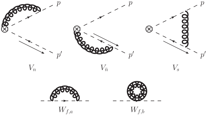
Refer to caption
Figure 7: Non-vanishing EFT diagrams for the computation of the hard matching coefficient, soft mass mode bin subtractions are implied for the collinear diagrams.

Following Eq. (74) we can obtain the 𝒪(αs2CFTF)𝒪superscriptsubscript𝛼𝑠2subscript𝐶𝐹subscript𝑇𝐹{\cal O}(\alpha_{s}^{2}C_{\!F}T_{F}) secondary massive quark form factor corrections relevant for the hard current matching calculation with the on-shell subtraction for the strong coupling by the relation

FQCD(SCET)(2,OS)(Q,m,μ)=subscriptsuperscript𝐹2OSQCDSCET𝑄𝑚𝜇absent\displaystyle F^{(2,\rm OS)}_{\rm QCD(SCET)}\!(Q,m,\mu)= 1πdM2M2FM,QCD(SCET)(1)(Q,M,μ)1𝜋dsuperscript𝑀2superscript𝑀2subscriptsuperscript𝐹1𝑀QCDSCET𝑄𝑀𝜇\displaystyle\,\frac{1}{\pi}\!\int\!\frac{\mathrm{d}M^{2}}{M^{2}}F^{(1)}_{M,\rm QCD(SCET)}\!(Q,M,\mu)
×Im[Π(m2,M2)],absentImdelimited-[]Πsuperscript𝑚2superscript𝑀2\displaystyle\times\mathrm{Im}\!\left[\Pi(m^{2},M^{2})\right], (77)

where FM,QCD(1)subscriptsuperscript𝐹1𝑀QCDF^{(1)}_{M,\rm QCD} (FM,SCET(1)subscriptsuperscript𝐹1𝑀SCETF^{(1)}_{M,\rm SCET}) denotes the one-loop massive gluon form factor in QCD (SCET). FQCD(2,OS)subscriptsuperscript𝐹2OSQCDF^{(2,\rm OS)}_{\rm QCD} is both IR- and UV-finite, has been computed in Refs. Kniehl1990 ; Hoang:1995fr and is equivalent to FQCD(nl,2)subscriptsuperscript𝐹subscript𝑛𝑙2QCDF^{(n_{l},2)}_{\rm QCD} given in Eq. (III.1). The massive gluon form factor diagrams in SCET are displayed in Fig. 7, have been computed in Refs. Gritschacher:thesis ; Gritschacher:2013pha and read in d𝑑d dimensions121212Here we have corrected a typo in Eq. (71) of Ref. Gritschacher:2013pha concerning the factor (1)2d/2superscript12𝑑2(-1)^{2-d/2} appearing in Eq. (IV.2). For d4𝑑4d\rightarrow 4 both expressions give the same terms up to terms of 𝒪(ϵ)𝒪italic-ϵ\mathcal{O}(\epsilon).

FM,SCET(1)(Q,M,μ)=αsCF2πΓ(2d2)(μ2eγEM2)2d2subscriptsuperscript𝐹1𝑀SCET𝑄𝑀𝜇subscript𝛼𝑠subscript𝐶𝐹2𝜋Γ2𝑑2superscriptsuperscript𝜇2superscript𝑒subscript𝛾𝐸superscript𝑀22𝑑2\displaystyle F^{(1)}_{M,\rm SCET}(Q,M,\mu)=\frac{\alpha_{s}C_{\!F}}{2\pi}\Gamma\bigg{(}2-\frac{d}{2}\bigg{)}\Big{(}\frac{\mu^{2}e^{\gamma_{E}}}{M^{2}}\Big{)}^{2-\frac{d}{2}}
×[Hd21(1)2d/2Γ(d2)Γ(1d2)\displaystyle\times\!\bigg{[}H_{\frac{d}{2}-1}-(-1)^{2-d/2}\,\Gamma\bigg{(}\frac{d}{2}\bigg{)}\Gamma\bigg{(}1-\frac{d}{2}\bigg{)}
46d+d2d(d2)+ln(M2Q2)],\displaystyle-\frac{4-6\,d+d^{2}}{d\,(d-2)}+\textrm{ln}{\bigg{(}\frac{M^{2}}{Q^{2}}\bigg{)}}\bigg{]}\,, (78)

where Hnsubscript𝐻𝑛H_{n} denotes the n𝑛n-th Harmonic Number. To avoid double counting and achieve gauge invariance it is crucial to subtract the soft-bin contributions, which arise from the soft scaling regions of the collinear diagrams. The collinear diagrams Vnsubscript𝑉𝑛V_{n}, Vn¯subscript𝑉¯𝑛V_{\bar{n}}, their soft-bin subtractions and the soft diagram Vssubscript𝑉𝑠V_{s} in Fig. 7 are for themselves not fully regularized in dimensional regularization due to rapidity divergences. These cancel in the sum of all diagrams and leave behind the rapidity logarithm ln(M2/Q2)lnsuperscript𝑀2superscript𝑄2\textrm{ln}(M^{2}/Q^{2}). Due to the finite gluon mass the soft-bin contributions are essential and non-vanishing for a general regularization of the rapidity singularities. Interestingly, this logarithm cancels in the difference of FM,QCD(1)subscriptsuperscript𝐹1𝑀QCDF^{(1)}_{M,\rm QCD} and FM,SCET(1)subscriptsuperscript𝐹1𝑀SCETF^{(1)}_{M,\rm SCET} so that there is no corresponding rapidity logarithm in the 𝒪(αs2CFTF)𝒪superscriptsubscript𝛼𝑠2subscript𝐶𝐹subscript𝑇𝐹\mathcal{O}(\alpha_{s}^{2}C_{\!F}T_{F}) secondary massive quark corrections to the hard current matching coefficient at the scale μHQsimilar-tosubscript𝜇𝐻𝑄\mu_{H}\sim Q. Thus the rapidity singularities that arise in the SCET form factor computation do not leave any trace in the hard current matching coefficient.

Carrying out the convolution in Eq. (77) in d=42ϵ𝑑42italic-ϵd=4-2\epsilon dimensions and expanding in ϵitalic-ϵ\epsilon we obtain (x2m2/(Q2+i 0)superscript𝑥2superscript𝑚2superscript𝑄2𝑖 0x^{2}\equiv m^{2}/(Q^{2}+i\,0), LQln[(Q2+i 0)/μ2]subscript𝐿𝑄lndelimited-[]superscript𝑄2𝑖 0superscript𝜇2L_{-Q}\equiv\textrm{ln}[-(Q^{2}+i\,0)/\mu^{2}], αs=αs(nl)(μ)subscript𝛼𝑠superscriptsubscript𝛼𝑠subscript𝑛𝑙𝜇\alpha_{s}=\alpha_{s}^{(n_{l})}(\mu))

FSCET(2,OS)(Q,m,μ)=αs2CFTF(4π)2{2ϵ3+1ϵ2[83ln(x2)\displaystyle F^{(2,\rm OS)}_{\rm SCET}(Q,m,\mu)=\frac{\alpha_{s}^{2}C_{\!F}T_{F}}{(4\pi)^{2}}\left\{\frac{2}{\epsilon^{3}}+\frac{1}{\epsilon^{2}}\left[-\frac{8}{3}\,\textrm{ln}{(-x^{2})}\right.\right.
4LQ+89]+1ϵ[43ln2(x2)+163ln(x2)LQ\displaystyle-\left.4\,L_{-Q}+\frac{8}{9}\right]+\frac{1}{\epsilon}\left[\frac{4}{3}\,\textrm{ln}^{2}{(-x^{2})}+\frac{16}{3}\,\textrm{ln}(-x^{2})\,L_{-Q}\right.
+4LQ24ln(x2)169LQ(6527+π29)]83LQ3\displaystyle+\!\left.4\,L_{-Q}^{2}-4\,\textrm{ln}{(-x^{2})}-\frac{16}{9}\,L_{-Q}-\left(\frac{65}{27}+\frac{\pi^{2}}{9}\right)\!\right]\!-\frac{8}{3}\,L_{-Q}^{3}
163ln(x2)LQ283ln2(x2)LQ+569ln2(x2)163lnsuperscript𝑥2superscriptsubscript𝐿𝑄283superscriptln2superscript𝑥2subscript𝐿𝑄569superscriptln2superscript𝑥2\displaystyle-\frac{16}{3}\,\textrm{ln}{(-x^{2})}L_{-Q}^{2}-\frac{8}{3}\,\textrm{ln}^{2}{(-x^{2})}L_{-Q}+\frac{56}{9}\textrm{ln}^{2}{(-x^{2})}
+8ln(x2)LQ+169LQ2+(24227+4π29)ln(x2)8lnsuperscript𝑥2subscript𝐿𝑄169superscriptsubscript𝐿𝑄2242274superscript𝜋29lnsuperscript𝑥2\displaystyle+8\,\textrm{ln}{(-x^{2})}L_{-Q}+\frac{16}{9}L_{-Q}^{2}+\left(\frac{242}{27}+\frac{4\pi^{2}}{9}\right)\!\textrm{ln}{(-x^{2})}
+(13027+2π29)LQ+87554+8π29203ζ3}.\displaystyle+\left.\left(\frac{130}{27}+\frac{2\pi^{2}}{9}\right)\!L_{-Q}+\frac{875}{54}+\frac{8\pi^{2}}{9}-\frac{20}{3}\,\zeta_{3}\right\}\,. (79)

Since FQCD(2,OS)subscriptsuperscript𝐹2OSQCDF^{(2,\rm OS)}_{\rm QCD} and FSCET(2,OS)subscriptsuperscript𝐹2OSSCETF^{(2,\rm OS)}_{\rm SCET} have been computed with the subtracted dispersion relation they correspond to expressions in the nlsubscript𝑛𝑙n_{l}-flavor scheme for the strong coupling. To switch to the (nl+1subscript𝑛𝑙1n_{l}+1)-flavor scheme one has to add the MS¯¯MS\overline{\rm MS}-subtracted vacuum polarization function at zero-momentum times the corresponding one-loop form factor,

FQCD(SCET)(2)(Q,m,μ,Δ)=FQCD(SCET)(2,OS)(Q,m,μ)subscriptsuperscript𝐹2QCDSCET𝑄𝑚𝜇Δsubscriptsuperscript𝐹2OSQCDSCET𝑄𝑚𝜇\displaystyle F^{(2)}_{\rm QCD(SCET)}(Q,m,\mu,\Delta)=F^{(2,\rm OS)}_{\rm QCD(SCET)}(Q,m,\mu)
(Π(m2,0)αsTF3π1ϵ)FQCD(SCET)(1)(Q,μ,Δ),Πsuperscript𝑚20subscript𝛼𝑠subscript𝑇𝐹3𝜋1italic-ϵsubscriptsuperscript𝐹1QCDSCET𝑄𝜇Δ\displaystyle-\left(\Pi(m^{2},0)-\frac{\alpha_{s}T_{F}}{3\pi}\,\frac{1}{\epsilon}\right)\!F^{(1)}_{\rm QCD(SCET)}(Q,\mu,\Delta)\,, (80)

where FQCD(1)subscriptsuperscript𝐹1QCDF^{(1)}_{\rm QCD} (FSCET(1)subscriptsuperscript𝐹1SCETF^{(1)}_{\rm SCET}) is the massless gluon one-loop QCD (SCET) form factor calculated with an IR regulator ΔΔ\Delta. To obtain the matching coefficient we should in principle first renormalize both quantities and then calculate their difference where the dependence on ΔΔ\Delta cancels. Since the QCD current is UV finite, it is convenient to revert this procedure, i.e. to first determine the difference of the unrenormalized quantities and renormalize the UV divergences in the SCET contribution at the very end. In this way the cancellation of the IR divergences can be made explicit from the beginning. The difference of the massless gluon one-loop QCD and SCET form factors has the form 131313Using dimensional regularization for both UV and IR divergences the SCET form factor for massless gluons vanishes identically.

FQCD(1)(Q,μ)FSCET(1)(Q,μ)=αsCF4π(μ2eγEQ2)2d2subscriptsuperscript𝐹1QCD𝑄𝜇subscriptsuperscript𝐹1SCET𝑄𝜇subscript𝛼𝑠subscript𝐶𝐹4𝜋superscriptsuperscript𝜇2superscript𝑒subscript𝛾𝐸superscript𝑄22𝑑2\displaystyle F^{(1)}_{\rm QCD}(Q,\mu)-F^{(1)}_{\rm SCET}(Q,\mu)=\frac{\alpha_{s}C_{\!F}}{4\pi}\!\left(\!-\,\frac{\mu^{2}e^{\gamma_{E}}}{Q^{2}}\right)^{\!\!2-\frac{d}{2}}
×d27d+16d4Γ(2d2)Γ(d21)2Γ(d2).absentsuperscript𝑑27𝑑16𝑑4Γ2𝑑2Γsuperscript𝑑212Γ𝑑2\displaystyle\times\frac{d^{2}-7d+16}{d-4}\,\frac{\Gamma\!\left(2-\frac{d}{2}\right)\Gamma\!\left(\frac{d}{2}-1\right)^{2}}{\Gamma(d-2)}\,. (81)

The additional term corresponding to the change from the nlsubscript𝑛𝑙n_{l}- to the (nl+1subscript𝑛𝑙1n_{l}+1)-flavor scheme thus reads

δFOSMS¯(Q,m,μ)𝛿superscript𝐹OS¯MS𝑄𝑚𝜇\displaystyle\delta F^{{\rm OS}\rightarrow\overline{\rm MS}}(Q,m,\mu)
=(Π(m2,0)αsTF3π1ϵ)(FQCD(1)FSCET(1))absentΠsuperscript𝑚20subscript𝛼𝑠subscript𝑇𝐹3𝜋1italic-ϵsubscriptsuperscript𝐹1QCDsubscriptsuperscript𝐹1SCET\displaystyle=-\left(\Pi(m^{2},0)-\frac{\alpha_{s}T_{F}}{3\pi}\,\frac{1}{\epsilon}\right)\!\left(F^{(1)}_{\rm QCD}-F^{(1)}_{\rm SCET}\right)
=αs2CFTF(4π)2{1ϵ2[83ln(x2)83LQ]\displaystyle=\frac{\alpha_{s}^{2}C_{\!F}T_{F}}{(4\pi)^{2}}\bigg{\{}\frac{1}{\epsilon^{2}}\left[-\frac{8}{3}\,\textrm{ln}(-x^{2})-\frac{8}{3}\,L_{-Q}\right]
+1ϵ[43ln2(x2)+163ln(x2)LQ+4LQ2\displaystyle+\frac{1}{\epsilon}\bigg{[}\frac{4}{3}\,\textrm{ln}^{2}(-x^{2})+\frac{16}{3}\,\textrm{ln}(-x^{2})L_{-Q}+4\,L_{-Q}^{2}
4ln(x2)4LQ+2π29]49ln3(x2)\displaystyle-4\,\textrm{ln}(-x^{2})-4\,L_{-Q}+\frac{2\pi^{2}}{9}\bigg{]}\!-\frac{4}{9}\,\textrm{ln}^{3}(-x^{2})
83ln2(x2)LQ163ln(x2)LQ2289LQ383superscriptln2superscript𝑥2subscript𝐿𝑄163lnsuperscript𝑥2superscriptsubscript𝐿𝑄2289superscriptsubscript𝐿𝑄3\displaystyle-\frac{8}{3}\,\textrm{ln}^{2}(-x^{2})L_{-Q}-\frac{16}{3}\,\textrm{ln}(-x^{2})L_{-Q}^{2}-\frac{28}{9}\,L_{-Q}^{3}
+2ln2(x2)+8ln(x2)LQ+6LQ22superscriptln2superscript𝑥28lnsuperscript𝑥2subscript𝐿𝑄6superscriptsubscript𝐿𝑄2\displaystyle+2\,\textrm{ln}^{2}(-x^{2})+8\,\textrm{ln}(-x^{2})L_{-Q}+6\,L_{-Q}^{2}
323ln(x2)(323+2π29)LQ+π2389ζ3}.\displaystyle-\frac{32}{3}\,\textrm{ln}(-x^{2})-\bigg{(}\frac{32}{3}+\frac{2\pi^{2}}{9}\bigg{)}L_{-Q}+\frac{\pi^{2}}{3}-\frac{8}{9}\,\zeta_{3}\bigg{\}}\,. (82)

Combining all contributions and including the MS¯¯MS\overline{\rm MS} current counterterm contribution ZC,nf=1(nl+1,2)subscriptsuperscript𝑍subscript𝑛𝑙12𝐶subscript𝑛𝑓1Z^{(n_{l}+1,2)}_{C,n_{\!f}=1} given in Eq. (5), the result for the 𝒪(αs2CFTF)𝒪superscriptsubscript𝛼𝑠2subscript𝐶𝐹subscript𝑇𝐹\mathcal{O}(\alpha_{s}^{2}C_{\!F}T_{F}) secondary massive quark contributions to the hard current coefficient in the (nl+1subscript𝑛𝑙1n_{l}+1)-flavor scheme reads (αs=αs(nl+1)(μ)subscript𝛼𝑠superscriptsubscript𝛼𝑠subscript𝑛𝑙1𝜇\alpha_{s}=\alpha_{s}^{(n_{l}+1)}(\mu))

δC(nl+1)(Q,m,μ)=FQCD(2,OS)(Q,m)FSCET(2,OS)(Q,m,μ)𝛿superscript𝐶subscript𝑛𝑙1𝑄𝑚𝜇subscriptsuperscript𝐹2OSQCD𝑄𝑚subscriptsuperscript𝐹2OSSCET𝑄𝑚𝜇\displaystyle\delta C^{(n_{l}+1)}(Q,m,\mu)=F^{(2,\rm OS)}_{\rm QCD}(Q,m)-F^{(2,\rm OS)}_{\rm SCET}(Q,m,\mu)
+δFOSMS¯(Q,m,μ)ZC,nf=1(nl+1,2)(Q,μ),𝛿superscript𝐹OS¯MS𝑄𝑚𝜇subscriptsuperscript𝑍subscript𝑛𝑙12𝐶subscript𝑛𝑓1𝑄𝜇\displaystyle+\delta F^{{\rm OS}\rightarrow\overline{\rm MS}}(Q,m,\mu)-Z^{(n_{l}+1,2)}_{C,n_{\!f}=1}(Q,\mu)\,, (83)

Inserting Eqs. (5), (IV.2), and (IV.2) and subtracting from Eq. (83) the massless limit of Eq. (4) for one single flavor we obtain the mass corrections to the form factor given in Eq. (35). We see from the result of Eq. (III.2) that the SCET matching procedure in the (nl+1subscript𝑛𝑙1n_{l}+1)-flavor scheme does in principle nothing other than exactly subtracting the asymptotic massless limit from the full QCD on-shell form factor correction.

IV.3 Thrust Jet Function

Refer to caption
Figure 8: Non-vanishing EFT diagrams for the computation of the jet function. The required soft mass mode bin subtractions are implicit. Concerning Jasubscript𝐽𝑎J_{a}, the right-symmetric diagram also has to be taken into account.

The calculation of the 𝒪(αs2CFTF)𝒪superscriptsubscript𝛼𝑠2subscript𝐶𝐹subscript𝑇𝐹{\cal O}(\alpha_{s}^{2}C_{\!F}T_{F}) secondary massive quark corrections to the jet function in the (nl+1subscript𝑛𝑙1n_{l}+1)-flavor scheme goes along the lines of the hard current coefficient. The 𝒪(αs)𝒪subscript𝛼𝑠\mathcal{O}(\alpha_{s}) corrections to the jet function due to a massive gauge boson with QCD vector coupling have the form Gritschacher:thesis ; Gritschacher:2013pha 141414We consider directly the corrections to the total thrust jet function, which are exactly twice the contributions for the function of a single jet.

δJM(1)(s,M,μ)=δJM,virt(1)(s,M,μ)+δJM,real(1)(s,M).𝛿superscriptsubscript𝐽𝑀1𝑠𝑀𝜇𝛿superscriptsubscript𝐽𝑀virt1𝑠𝑀𝜇𝛿superscriptsubscript𝐽𝑀real1𝑠𝑀\displaystyle\!\!\delta J_{M}^{(1)}(s,M,\mu)=\delta J_{M,\rm virt}^{(1)}(s,M,\mu)+\delta J_{M,\rm real}^{(1)}(s,M). (84)

The distributive part δJM,virt(1)𝛿superscriptsubscript𝐽𝑀virt1\delta J_{M,\rm virt}^{(1)} corresponds to virtual radiation of the massive gauge boson and the full expression in d𝑑d dimensions reads

μ2δJM,virt(1)(s,M,μ)=2αsCFπΓ(2d2)(μ2eγEM2)2d2superscript𝜇2𝛿superscriptsubscript𝐽𝑀virt1𝑠𝑀𝜇2subscript𝛼𝑠subscript𝐶𝐹𝜋Γ2𝑑2superscriptsuperscript𝜇2superscript𝑒subscript𝛾𝐸superscript𝑀22𝑑2\displaystyle\mu^{2}\delta J_{M,\rm virt}^{(1)}(s,M,\mu)=\frac{2\alpha_{s}C_{\!F}}{\pi}\Gamma\bigg{(}2-\frac{d}{2}\bigg{)}\!\bigg{(}\frac{\mu^{2}e^{\gamma_{E}}}{M^{2}}\bigg{)}^{2-\frac{d}{2}}
×{[Hd21H1d2+ln(M2μ2)+2d2d]δ(s¯)\displaystyle\times\left\{\left[H_{\frac{d}{2}-1}-H_{1-\frac{d}{2}}+\textrm{ln}{\left(\frac{M^{2}}{\mu^{2}}\right)}+\frac{2-d}{2d}\,\right]\!\delta(\bar{s})\right.
[θ(s¯)s¯]+}.\displaystyle\left.-\left[\frac{\theta(\bar{s})}{\bar{s}}\right]_{+}\right\}\,. (85)

The UV- and IR-finite real radiation contribution δJM,real(1)𝛿superscriptsubscript𝐽𝑀real1\delta J_{M,\rm real}^{(1)} can for our purposes be evaluated for d=4𝑑4d=4 since it does not require any regularization for the convolution in the subtracted dispersion relation. It reads

μ2δJM,real(1)(s,M)=αsCF2πμ2θ(sM2)superscript𝜇2𝛿superscriptsubscript𝐽𝑀real1𝑠𝑀subscript𝛼𝑠subscript𝐶𝐹2𝜋superscript𝜇2𝜃𝑠superscript𝑀2\displaystyle\mu^{2}\delta J_{M,\rm real}^{(1)}(s,M)=\frac{\alpha_{s}C_{\!F}}{2\pi}\mu^{2}\theta\left(s-M^{2}\right)
×{(M2s)(3s+M2)s3+4sln(sM2)}.absentsuperscript𝑀2𝑠3𝑠superscript𝑀2superscript𝑠34𝑠ln𝑠superscript𝑀2\displaystyle\times\left\{\frac{(M^{2}-s)(3s+M^{2})}{s^{3}}+\frac{4}{s}\,\textrm{ln}{\left(\frac{s}{M^{2}}\right)}\right\}. (86)

The calculation of δJM(1)𝛿superscriptsubscript𝐽𝑀1\delta J_{M}^{(1)} involves the collinear diagrams in Fig. 8, where the corresponding soft-bin subtractions are implied and contribute only to δJM,virt(1)𝛿superscriptsubscript𝐽𝑀virt1\delta J_{M,\rm virt}^{(1)}. The soft-bin subtractions are crucial for gauge invariance as well as for a cancellation of all rapidity singularities Gritschacher:2013pha . As a remnant of this cancellation we get a rapidity logarithm ln(M2/μ2)ln(M2/s)similar-tolnsuperscript𝑀2superscript𝜇2lnsuperscript𝑀2𝑠\textrm{ln}(M^{2}/\mu^{2})\sim\textrm{ln}(M^{2}/s) in δJM,virt(1)𝛿superscriptsubscript𝐽𝑀virt1\delta J_{M,\rm virt}^{(1)} in Eq. (85). For M2smuch-less-thansuperscript𝑀2𝑠M^{2}\ll s a corresponding logarithm arises in the real radiation term δJM,real(1)𝛿superscriptsubscript𝐽𝑀real1\delta J_{M,\rm real}^{(1)} in Eq. (86) which cancels the rapidity logarithm from δJM,virt(1)𝛿superscriptsubscript𝐽𝑀virt1\delta J_{M,\rm virt}^{(1)}. We emphasize, however, that in the calculation of δJM,real(1)𝛿superscriptsubscript𝐽𝑀real1\delta J_{M,\rm real}^{(1)} rapidity divergences do not arise anywhere. These properties are also inherited to the 𝒪(αs2CFTF)𝒪superscriptsubscript𝛼𝑠2subscript𝐶𝐹subscript𝑇𝐹\mathcal{O}(\alpha_{s}^{2}C_{\!F}T_{F}) massive quark corrections discussed in the following.

The 𝒪(αs2CFTF)𝒪superscriptsubscript𝛼𝑠2subscript𝐶𝐹subscript𝑇𝐹{\cal O}(\alpha_{s}^{2}C_{\!F}T_{F}) unrenormalized massive quark corrections to the jet function in the nlsubscript𝑛𝑙n_{l}-flavor scheme for αssubscript𝛼𝑠\alpha_{s} can be obtained with the subtracted dispersion relation

δJm(2,OS)(s,m,μ)=δJm(OS,virt)(s,m,μ)+δJmreal(s,m)𝛿subscriptsuperscript𝐽2OS𝑚𝑠𝑚𝜇𝛿subscriptsuperscript𝐽OSvirt𝑚𝑠𝑚𝜇𝛿subscriptsuperscript𝐽real𝑚𝑠𝑚\displaystyle\delta J^{(2,\rm OS)}_{m}(s,m,\mu)=\delta J^{(\rm OS,virt)}_{m}(s,m,\mu)+\delta J^{\rm real}_{m}(s,m)
=1πdM2M2δJM(1)(s,M,μ)Im[Π(m2,M2)].absent1𝜋dsuperscript𝑀2superscript𝑀2𝛿superscriptsubscript𝐽𝑀1𝑠𝑀𝜇Imdelimited-[]Πsuperscript𝑚2superscript𝑀2\displaystyle=\frac{1}{\pi}\int\frac{\mathrm{d}M^{2}}{M^{2}}\,\delta J_{M}^{(1)}(s,M,\mu)\,\mathrm{Im}\!\left[\Pi(m^{2},M^{2})\right]\,. (87)

The convolution is performed separately for the d𝑑d-dimensional virtual terms in Eq. (85) and the four-dimensional threshold term in Eq. (86), where for the latter no divergences arise in the M𝑀M-integration and thus the d=4𝑑4d=4 version of the absorptive part of the vacuum polarization function in Eq. (IV.1) can be used. This yields Eq. (III.3) for the real radiation term δJmreal𝛿subscriptsuperscript𝐽real𝑚\delta J^{\rm real}_{m} and (Lm=ln(m2/μ2),αs=αs(nl)(μ)formulae-sequencesubscript𝐿𝑚lnsuperscript𝑚2superscript𝜇2subscript𝛼𝑠superscriptsubscript𝛼𝑠subscript𝑛𝑙𝜇L_{m}=\textrm{ln}(m^{2}/\mu^{2}),\alpha_{s}=\alpha_{s}^{(n_{l})}(\mu))

μ2δJm(OS,virt)(s,m,μ)=αs2CFTF(4π)2{[8ϵ3\displaystyle\mu^{2}\delta J^{(\rm OS,\rm virt)}_{m}(s,m,\mu)=\frac{\alpha_{s}^{2}C_{\!F}T_{F}}{(4\pi)^{2}}\left\{\left[\frac{8}{\epsilon^{3}}\right.\right.
+1ϵ2(323Lm49)+1ϵ(163Lm28Lm24227+4π29)1superscriptitalic-ϵ2323subscript𝐿𝑚491italic-ϵ163superscriptsubscript𝐿𝑚28subscript𝐿𝑚242274superscript𝜋29\displaystyle+\frac{1}{\epsilon^{2}}\left(-\frac{32}{3}\,L_{m}-\frac{4}{9}\right)+\frac{1}{\epsilon}\left(\frac{16}{3}\,L_{m}^{2}-8\,L_{m}-\frac{242}{27}+\frac{4\pi^{2}}{9}\right)
+1529Lm2+93227Lm+153127+38π227643ζ3]δ(s¯)\displaystyle\left.+\frac{152}{9}\,L_{m}^{2}+\frac{932}{27}\,L_{m}+\frac{1531}{27}+\frac{38\pi^{2}}{27}-\frac{64}{3}\,\zeta_{3}\right]\!\delta(\bar{s})
+[163ϵ2+1ϵ(323Lm+809)323Lm21609Lm\displaystyle+\left[-\frac{16}{3\epsilon^{2}}+\frac{1}{\epsilon}\left(\frac{32}{3}\,L_{m}+\frac{80}{9}\right)-\frac{32}{3}\,L_{m}^{2}-\frac{160}{9}\,L_{m}\right.
448278π29][θ(s¯)s¯]+}.\displaystyle-\left.\left.\frac{448}{27}-\frac{8\pi^{2}}{9}\right]\!\!\left[\frac{\theta(\bar{s})}{\bar{s}}\right]_{+}\right\}\,. (88)

We switch to the (nl+1subscript𝑛𝑙1n_{l}+1)-flavor scheme for αssubscript𝛼𝑠\alpha_{s} by adding the MS¯¯MS\overline{\rm MS}-renormalized Π(0)Π0\Pi(0) times the (unrenormalized) massless one loop contribution to the jet function which reads

Jbare(1)(s,μ)=αsCF2π1s(μ2eγEs)2d2d+4d4Γ(d2)Γ(d2).subscriptsuperscript𝐽1bare𝑠𝜇subscript𝛼𝑠subscript𝐶𝐹2𝜋1𝑠superscriptsuperscript𝜇2superscript𝑒subscript𝛾𝐸𝑠2𝑑2𝑑4𝑑4Γ𝑑2Γ𝑑2\displaystyle\!\!\!\!J^{(1)}_{\rm bare}(s,\mu)=\frac{\alpha_{s}C_{\!F}}{2\pi}\frac{1}{s}\Big{(}\frac{\mu^{2}e^{\gamma_{E}}}{s}\Big{)}^{2-\frac{d}{2}}\frac{d+4}{d-4}\,\frac{\Gamma\left(\frac{d}{2}\right)}{\Gamma\left(d-2\right)}\,. (89)

Thus the corresponding contribution needed to change from the nlsubscript𝑛𝑙n_{l} to the (nl+1subscript𝑛𝑙1n_{l}+1)-flavor scheme reads

δJmOSMS¯(s,m,μ)𝛿subscriptsuperscript𝐽OS¯MS𝑚𝑠𝑚𝜇\displaystyle\delta J^{{\rm OS}\rightarrow\overline{\rm MS}}_{m}(s,m,\mu)
=(Π(m2,0)αsTF3π1ϵ)Jbare(1)(s,μ)absentΠsuperscript𝑚20subscript𝛼𝑠subscript𝑇𝐹3𝜋1italic-ϵsubscriptsuperscript𝐽1bare𝑠𝜇\displaystyle=-\,\bigg{(}\Pi(m^{2},0)-\frac{\alpha_{s}T_{F}}{3\pi}\,\frac{1}{\epsilon}\bigg{)}\,J^{(1)}_{\rm bare}(s,\mu)
=αs2CFTF(4π)2{[323ϵ2Lm+1ϵ(163Lm2+8Lm8π29)\displaystyle=\frac{\alpha_{s}^{2}C_{\!F}T_{F}}{(4\pi)^{2}}\left\{\left[\frac{32}{3\epsilon^{2}}\,L_{m}+\frac{1}{\epsilon}\left(-\frac{16}{3}\,L_{m}^{2}+8\,L_{m}-\frac{8\pi^{2}}{9}\right)\right.\right.
+169Lm34Lm2+(56316π29)Lm2π23+329ζ3]δ(s¯)\displaystyle+\left.\!\frac{16}{9}L_{m}^{3}-4\,L_{m}^{2}+\bigg{(}\frac{56}{3}-\frac{16\pi^{2}}{9}\bigg{)}L_{m}-\frac{2\pi^{2}}{3}+\frac{32}{9}\,\zeta_{3}\right]\!\delta(\bar{s})
+[323ϵLm+163Lm28Lm+8π29][θ(s¯)s¯]+delimited-[]323italic-ϵsubscript𝐿𝑚163superscriptsubscript𝐿𝑚28subscript𝐿𝑚8superscript𝜋29subscriptdelimited-[]𝜃¯𝑠¯𝑠\displaystyle+\left[-\frac{32}{3\epsilon}\,L_{m}+\frac{16}{3}\,L_{m}^{2}-8\,L_{m}+\frac{8\pi^{2}}{9}\right]\!\!\left[\frac{\theta(\bar{s})}{\bar{s}}\right]_{+}
+323Lm[θ(s¯)lns¯s¯]+}.\displaystyle+\left.\frac{32}{3}\,L_{m}\left[\frac{\theta(\bar{s})\,\textrm{ln}\,\bar{s}}{\bar{s}}\right]_{+}\right\}\,. (90)

Combining all contributions and renormalizing the result with the jet counterterm contribution ZJ,nf=1(nl+1,2)superscriptsubscript𝑍𝐽subscript𝑛𝑓1subscript𝑛𝑙12Z_{J,n_{\!f}=1}^{(n_{l}+1,2)} in Eq. (7) finally gives

δJmvirt(s,m,μ)=𝛿superscriptsubscript𝐽𝑚virt𝑠𝑚𝜇absent\displaystyle\delta J_{m}^{\rm virt}(s,m,\mu)= δJm(OS,virt)(s,m,μ)+δJmOSMS¯(s,m,μ)𝛿subscriptsuperscript𝐽OSvirt𝑚𝑠𝑚𝜇𝛿subscriptsuperscript𝐽OS¯MS𝑚𝑠𝑚𝜇\displaystyle\,\delta J^{({\rm OS,virt})}_{m}(s,m,\mu)+\delta J^{{\rm OS}\rightarrow\overline{\rm MS}}_{m}(s,m,\mu)
ZJ,nf=1(nl+1,2)(s,μ).superscriptsubscript𝑍𝐽subscript𝑛𝑓1subscript𝑛𝑙12𝑠𝜇\displaystyle-Z_{J,n_{\!f}=1}^{(n_{l}+1,2)}(s,\mu)\,. (91)

Inserting Eqs. (7), (IV.3), (IV.3) and subtracting from Eq. (IV.3) the massless limit of Eq. (II) for one single flavor we obtain the virtual massive quark corrections to the jet function given in Eq. (41).

V Renormalization Conditions, Threshold Corrections and Consistency Relations

In this section we discuss the RG properties of the individual ingredients of the factorization theorem, namely the hard current coefficient, the jet function and the soft function, rather than the factorization theorem as a whole. Since the hard coefficient and the jet and soft functions are gauge-invariant quantities, they can also be renormalized independently. This fact can be used to determine the threshold correction factors Csubscript𝐶\mathcal{M}_{C} for the hard coefficient (see Eq. (38)) and Jsubscript𝐽\mathcal{M}_{J} for the jet function (see Eq. (46)) as well as the threshold correction factor Ssubscript𝑆\mathcal{M}_{S} for the soft function (see Eq. (144)). The latter becomes relevant if one sets the final renormalization scale μ𝜇\mu above the soft scale and the RG evolution of the soft function crosses the massive quark threshold. Instead of using different effective theories that follow the strict guideline of having the massive quark modes either as fluctuating fields contributing to the RG evolution in the same way as the massless quarks or excluded completely (i.e. integrated out), we use only a single theory which contains the massive quark modes, but employs different renormalization conditions for the quantum corrections that arise from the massive quark modes. These renormalization conditions are either the MS¯¯MS\overline{\rm MS} prescription or an on-shell (or low-energy momentum subtraction) prescription. The former leads to the usual MS¯¯MS\overline{\rm MS} feature that massless quarks and the massive flavor all contribute to the RG evolution in the same way, so one uses the (nl+1subscript𝑛𝑙1n_{l}+1) running flavor scheme. The latter also subtracts finite and scale-dependent contributions such that the massive flavor does not lead to any contribution in the RG evolution, so there are only nlsubscript𝑛𝑙n_{l} running flavors. This concerns the strong coupling αssubscript𝛼𝑠\alpha_{s} (see Sec. IV.1) as well as the hard coefficient and the jet and soft functions.

Obviously the MS¯¯MS\overline{\rm MS} prescription is suitable to cover the situation where the quark mass becomes small (where “suitable” means that no large mass logarithms arise in the massless limit) and, as already demonstrated in Sec. IV, leads to results which give the known results for massless quarks in the limit m0𝑚0m\rightarrow 0. The on-shell prescription is suitable to cover the decoupling limit, such that the effects of the massive quark vanish in the infinite mass limit. The decoupling condition renders the finite subtraction unique for all calculations within SCET. This method of using different renormalization conditions for the RG evolution schemes with (nl+1subscript𝑛𝑙1n_{l}+1) and nlsubscript𝑛𝑙n_{l} running flavors also has the advantage that the kinematic thresholds of the jet and soft functions due to the quark mass are fully contained in them regardless of which type of renormalization scheme is used. This is unlike the case of using the effective theory method, where the massive quark is completely excluded from the nlsubscript𝑛𝑙n_{l}-flavor theory, and one is forced to take care of the fact that the real radiation thresholds are always located in the (nl+1subscript𝑛𝑙1n_{l}+1)-flavor theory.

The differences of the renormalized quantities w.r. to both of these renormalization prescriptions constitute threshold matching conditions that uniquely define the mass mode matching threshold correction factors Csubscript𝐶\mathcal{M}_{C}, Jsubscript𝐽\mathcal{M}_{J} and Ssubscript𝑆\mathcal{M}_{S}. Since the hard current coefficient, the jet and the soft functions are independent and in principle not tied to the particular factorization theorem for thrust, the important outcome is that the threshold correction factors can be determined from these quantities and do not rely on a separate perturbative calculation of the thrust distribution in full QCD. From the form of the factorization theorem for thrust we can therefore predict the singular 𝒪(αs2CFTF)𝒪superscriptsubscript𝛼𝑠2subscript𝐶𝐹subscript𝑇𝐹\mathcal{O}(\alpha_{s}^{2}C_{\!F}T_{F}) massive quark corrections to the thrust distribution in full fixed-order QCD. To our knowledge they have not been calculated in an explicit form before in the literature.

The fact that the hard coefficients, the jet and soft functions and the massive quark threshold corrections factors that appear in the factorization theorems in the four scenarios (in schemes with either nlsubscript𝑛𝑙n_{l} or nl+1subscript𝑛𝑙1n_{l}+1 running flavors) are conceptually connected through different choices of renormalization schemes and not related in any way to expansions in either small or large quantities makes it evident that the predictions of the different factorization theorems at their respective borders of validity have an overlap region and are continuous. 151515We mean continuity up to higher order perturbative corrections which are not enhanced by large logarithms.
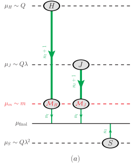
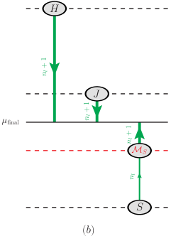
Refer to caption
Refer to caption
Refer to caption
Figure 9: Illustration of the different RG setups for scenario III (μJ>μm>μSsubscript𝜇𝐽subscript𝜇𝑚subscript𝜇𝑆\mu_{J}>\mu_{m}>\mu_{S}) leading to the consistency relations mentioned in the text. Shown are the cases where the final renormalization scale μfinalsubscript𝜇final\mu_{\rm final} satisfies (a) μm>μfinal>μSsubscript𝜇𝑚subscript𝜇finalsubscript𝜇𝑆\mu_{m}>\mu_{\rm final}>\mu_{S}, (b) μJ>μfinal>μmsubscript𝜇𝐽subscript𝜇finalsubscript𝜇𝑚\mu_{J}>\mu_{\rm final}>\mu_{m} and (c) μH>μfinal>μJsubscript𝜇𝐻subscript𝜇finalsubscript𝜇𝐽\mu_{H}>\mu_{\rm final}>\mu_{J}.

We believe that it is worth discussing this issue briefly in the following. In Sec. III we have discussed four scenarios one needs to distinguish for treating the possible hierarchies between the quark mass m𝑚m on the one side and the hard scale Q𝑄Q, the jet scale Qλsimilar-toabsent𝑄𝜆\sim Q\lambda and the soft scale Qλ2𝑄superscript𝜆2Q\lambda^{2} on the other. Concerning the power counting we may assume the canonical strong hierarchy between these scales (such as QmQλQλ2much-greater-than𝑄𝑚much-greater-than𝑄𝜆much-greater-than𝑄superscript𝜆2Q\gg m\gg Q\lambda\gg Q\lambda^{2}) when discussing the effective theory setup, the RG evolution, the results for hard current coefficient, jet and soft functions and the mass mode threshold corrections that result when the massive modes are integrated out. However, since the components of the factorization theorems are related simply by different choices of renormalization conditions, each factorization theorem also applies in cases where hierarchies involving the mass are only marginal or non-existent (such as QmQλQλ2much-greater-than𝑄𝑚greater-than-or-equivalent-to𝑄𝜆much-greater-than𝑄superscript𝜆2Q\gg m\gtrsim Q\lambda\gg Q\lambda^{2} or QmQλQλ2greater-than-or-equivalent-to𝑄𝑚much-greater-than𝑄𝜆much-greater-than𝑄superscript𝜆2Q\gtrsim m\gg Q\lambda\gg Q\lambda^{2}). In these cases the RG evolution between close-by scales is equivalent to a perturbative treatment, so that the factors of concern might be simply expanded out. Since this might be as well applied to the two neighboring scenarios within some range, we have continuity between the two descriptions, and the transition point where one switches between them can be picked freely within this range. This feature is very similar to (but distinguished from) the property that the scale μmsubscript𝜇𝑚\mu_{m} where the quark mass m𝑚m is integrated out can be picked freely within some range in a practical application. The freedom in these choices causes changes in the numerical predictions due to the truncation of the perturbative expansion and might contribute to estimating the remaining perturbative uncertainty.

The fact of having four different scales relevant for setting up the RG evolution (μHsubscript𝜇𝐻\mu_{H}, μJsubscript𝜇𝐽\mu_{J}, μSsubscript𝜇𝑆\mu_{S} and μmsubscript𝜇𝑚\mu_{m}) leads to another interesting feature related to the proliferation of possibilities to pick the final renormalization scale μ=μfinal𝜇subscript𝜇final\mu=\mu_{\rm final} to which the hard current coefficient, the jet function and the soft function are being evolved in the different factorization theorems. See Fig. 9 for an illustration of three equivalent choices for scenario III, where we display the situations in which μfinalsubscript𝜇final\mu_{\rm final} lies (a) between mass and soft scales, (b) between the jet and mass scales, and (c) between the hard and jet scales. The different possibilities and their equivalence concerning predictions is one of the deeper conceptual properties of factorization theorems. On the one hand, they imply the well-known consistency conditions between the RG evolution factors UC(nf)superscriptsubscript𝑈𝐶subscript𝑛𝑓U_{C}^{(n_{\!f})}, UJ(nf)superscriptsubscript𝑈𝐽subscript𝑛𝑓U_{J}^{(n_{\!f})} and US(nf)superscriptsubscript𝑈𝑆subscript𝑛𝑓U_{S}^{(n_{\!f})} for nf=nlsubscript𝑛𝑓subscript𝑛𝑙n_{\!f}=n_{l} and nf=nl+1subscript𝑛𝑓subscript𝑛𝑙1n_{\!f}=n_{l}+1, see Eq. (24). However, in the context of the RG evolution crossing a massive quark threshold they also imply a consistency relation between the mass mode threshold matching correction factors Csubscript𝐶\mathcal{M}_{C}, Jsubscript𝐽\mathcal{M}_{J} and Ssubscript𝑆\mathcal{M}_{S}. This can be used to gain interesting general insights into properties of mass singularities, and at the practical level, may be used as a non-trivial tool for consistency checks.

Apart from providing consistency checks of theoretical calculations, these relations also have computational power, as they can be used to calculate properties of gauge-invariant and independent field theoretic objects once it has become clear that they represent building blocks of a factorization theorem. In the case of thrust these building blocks are the hard (vector or axial) current coefficient, the jet function and the soft function. Hereby, one of the most interesting aspects is that the various building blocks can appear in different factorization theorems and one may gain insights into the mass-singularities of apparently unrelated quantities.

In the following subsections A-C we discuss the evolution and the mass mode threshold corrections for the hard current coefficient, the jet function and the soft function using the renormalization method described above. The calculations are fast and concise and are based on the 𝒪(αs2CFTF)𝒪superscriptsubscript𝛼𝑠2subscript𝐶𝐹subscript𝑇𝐹\mathcal{O}(\alpha_{s}^{2}C_{\!F}T_{F}) massive quark results given in Sec. IV. Using RG-invariance w.r. to the scale where one switches between nlsubscript𝑛𝑙n_{l}- and (nl+1subscript𝑛𝑙1n_{l}+1)-flavor schemes we also examine terms of 𝒪(αs3)𝒪superscriptsubscript𝛼𝑠3\mathcal{O}(\alpha_{s}^{3}) and 𝒪(αs4)𝒪superscriptsubscript𝛼𝑠4\mathcal{O}(\alpha_{s}^{4}) which are enhanced by rapidity logarithms and may be counted as 𝒪(αs2)𝒪superscriptsubscript𝛼𝑠2\mathcal{O}(\alpha_{s}^{2}) in the logarithmic counting αsln𝒪(1)similar-tosubscript𝛼𝑠ln𝒪1\alpha_{s}\textrm{ln}\sim\mathcal{O}(1). In subsection D we discuss the consistency conditions among the mass mode matching corrections Csubscript𝐶\mathcal{M}_{C}, Jsubscript𝐽\mathcal{M}_{J} and Ssubscript𝑆\mathcal{M}_{S}, and we also show that they are also relevant for the perturbative equivalence of the factorization theorems of neighboring scenarios in their overlap region. In subsection E we present the explicit result for the singular 𝒪(αs2CFTF)𝒪superscriptsubscript𝛼𝑠2subscript𝐶𝐹subscript𝑇𝐹\mathcal{O}(\alpha_{s}^{2}C_{\!F}T_{F}) massive quark correction of the thrust distribution in full QCD in the fixed-order expansion.

V.1 Current mass mode matching coefficient

The mass mode threshold factor C(Q,m,μm)subscript𝐶𝑄𝑚subscript𝜇𝑚\mathcal{M}_{C}(Q,m,\mu_{m}) arises when the RG evolution of the hard current coefficient crosses the massive quark threshold. In the following we describe how it is related to the renormalization conditions for the hard current. The bare and the renormalized current coefficients C(0)(Q,m,μ)superscript𝐶0𝑄𝑚𝜇C^{(0)}(Q,m,\mu) and C(nf)(Q,m,μ)superscript𝐶subscript𝑛𝑓𝑄𝑚𝜇C^{(n_{\!f})}(Q,m,\mu) are related to each other via

C(0)(Q,m,μ)=ZC(nf)(Q,m,μ)C(nf)(Q,m,μ),superscript𝐶0𝑄𝑚𝜇superscriptsubscript𝑍𝐶subscript𝑛𝑓𝑄𝑚𝜇superscript𝐶subscript𝑛𝑓𝑄𝑚𝜇\displaystyle C^{(0)}(Q,m,\mu)=Z_{C}^{(n_{\!f})}(Q,m,\mu)\,C^{(n_{\!f})}(Q,m,\mu)\,, (92)

where ZC(nf)(Q,m,μ)superscriptsubscript𝑍𝐶subscript𝑛𝑓𝑄𝑚𝜇Z_{C}^{(n_{\!f})}(Q,m,\mu) is the renormalization factor in a nfsubscript𝑛𝑓n_{\!f}-flavor scheme. In the following we will omit all 𝒪(αs2CF2)𝒪superscriptsubscript𝛼𝑠2superscriptsubscript𝐶𝐹2\mathcal{O}(\alpha_{s}^{2}C_{\!F}^{2}) and 𝒪(αs2CFCA)𝒪superscriptsubscript𝛼𝑠2subscript𝐶𝐹subscript𝐶𝐴\mathcal{O}(\alpha_{s}^{2}C_{\!F}C_{\!A}) terms, as they are irrelevant for our considerations. For scales μ>m𝜇𝑚\mu>m we use the (nl+1)subscript𝑛𝑙1(n_{l}+1)-flavor scheme, so we employ the MS¯¯MS\overline{\rm MS}-subtractions for the UV divergent contributions to the strong coupling and the current. The counterterm is mass independent and reads with the notation of section II

ZC(nl+1)(Q,μ)=1+ZC(nl+1,1)(Q,μ)+ZC,nl+1(nl+1,2)(Q,μ).superscriptsubscript𝑍𝐶subscript𝑛𝑙1𝑄𝜇1superscriptsubscript𝑍𝐶subscript𝑛𝑙11𝑄𝜇superscriptsubscript𝑍𝐶subscript𝑛𝑙1subscript𝑛𝑙12𝑄𝜇\displaystyle Z_{C}^{(n_{l}+1)}(Q,\mu)=1+Z_{C}^{(n_{l}+1,1)}(Q,\mu)+Z_{C,n_{l}+1}^{(n_{l}+1,2)}(Q,\mu)\,. (93)

The 𝒪(αs2CFTF)𝒪superscriptsubscript𝛼𝑠2subscript𝐶𝐹subscript𝑇𝐹\mathcal{O}(\alpha_{s}^{2}C_{\!F}T_{F}) contribution ZC,nl+1(nl+1,2)(Q,μ)superscriptsubscript𝑍𝐶subscript𝑛𝑙1subscript𝑛𝑙12𝑄𝜇Z_{C,n_{l}+1}^{(n_{l}+1,2)}(Q,\mu) is given in Eq. (5) with nf=nl+1subscript𝑛𝑓subscript𝑛𝑙1n_{\!f}=n_{l}+1, whereas the 𝒪(αs)𝒪subscript𝛼𝑠\mathcal{O}(\alpha_{s}) term reads (LQ=ln((Q2+i 0)/μ2)subscript𝐿𝑄lnsuperscript𝑄2𝑖 0superscript𝜇2L_{-Q}=\textrm{ln}(-(Q^{2}+i\,0)/\mu^{2}))

ZC(nl+1,1)(Q,μ)=αs(nl+1)(μ)CF4π(2ϵ23ϵ+2ϵLQ).superscriptsubscript𝑍𝐶subscript𝑛𝑙11𝑄𝜇superscriptsubscript𝛼𝑠subscript𝑛𝑙1𝜇subscript𝐶𝐹4𝜋2superscriptitalic-ϵ23italic-ϵ2italic-ϵsubscript𝐿𝑄\displaystyle Z_{C}^{(n_{l}+1,1)}(Q,\mu)\,=\,\frac{\alpha_{s}^{(n_{l}+1)}(\mu)C_{\!F}}{4\pi}\bigg{(}\!-\frac{2}{\epsilon^{2}}-\frac{3}{\epsilon}+\frac{2}{\epsilon}L_{-Q}\bigg{)}\,. (94)

Note that the contribution from the massive quark agrees with the one related to a massless flavor. The renormalized current coefficient reads

C(nl+1)(Q,m,μ)=superscript𝐶subscript𝑛𝑙1𝑄𝑚𝜇absent\displaystyle C^{(n_{l}+1)}(Q,m,\mu)=  1+C(nl+1,1)(Q,μ)+Cnl+1(nl+1,2)(Q,μ)1superscript𝐶subscript𝑛𝑙11𝑄𝜇subscriptsuperscript𝐶subscript𝑛𝑙12subscript𝑛𝑙1𝑄𝜇\displaystyle\,1+C^{(n_{l}+1,1)}(Q,\mu)+C^{(n_{l}+1,2)}_{n_{l}+1}(Q,\mu)
+δF(nl+1,2)(Q,m),𝛿superscript𝐹subscript𝑛𝑙12𝑄𝑚\displaystyle+\delta F^{(n_{l}+1,2)}(Q,m)\,, (95)

which is the one for the case m<Q𝑚𝑄m<Q (scenarios II, III and IV) given in Eq. (35). The massless result at 𝒪(αs)𝒪subscript𝛼𝑠\mathcal{O}(\alpha_{s}) reads

C(nl+1,1)(Q,μ)superscript𝐶subscript𝑛𝑙11𝑄𝜇\displaystyle C^{(n_{l}+1,1)}(Q,\mu)
=αs(nl+1)(μ)CF4π(LQ2+3LQ8+π26).absentsuperscriptsubscript𝛼𝑠subscript𝑛𝑙1𝜇subscript𝐶𝐹4𝜋superscriptsubscript𝐿𝑄23subscript𝐿𝑄8superscript𝜋26\displaystyle=\frac{\alpha_{s}^{(n_{l}+1)}(\mu)C_{\!F}}{4\pi}\left(-\,L_{-Q}^{2}+3\,L_{-Q}-8+\frac{\pi^{2}}{6}\right)\,. (96)

In the nlsubscript𝑛𝑙n_{l}-flavor scheme, we intend to implement the renormalization condition that the massive quark corrections vanish for Qμmsimilar-to𝑄𝜇much-less-than𝑚Q\sim\mu\ll m. Following the computation described in Sec. IV.2, we now do not include the scheme change contribution δFOSMS¯𝛿superscript𝐹OS¯MS\delta F^{{\rm OS}\rightarrow\overline{\rm MS}}, which implies that we use αs(nl)superscriptsubscript𝛼𝑠subscript𝑛𝑙\alpha_{s}^{(n_{l})}, i.e. the nlsubscript𝑛𝑙n_{l}-flavor scheme for the strong coupling. The resulting expressions for the counterterm and the renormalized current coefficient read

ZC(nl)(Q,μ)=superscriptsubscript𝑍𝐶subscript𝑛𝑙𝑄𝜇absent\displaystyle Z_{C}^{(n_{l})}(Q,\mu)=  1+ZC(nl,1)(Q,μ)+ZC,nl(nl,2)(Q,μ)1superscriptsubscript𝑍𝐶subscript𝑛𝑙1𝑄𝜇superscriptsubscript𝑍𝐶subscript𝑛𝑙subscript𝑛𝑙2𝑄𝜇\displaystyle\,1+Z_{C}^{(n_{l},1)}(Q,\mu)+Z_{C,n_{l}}^{(n_{l},2)}(Q,\mu)
+ZC,OS(nl,2)(Q,m,μ),subscriptsuperscript𝑍subscript𝑛𝑙2𝐶OS𝑄𝑚𝜇\displaystyle+Z^{(n_{l},2)}_{C,\rm OS}(Q,m,\mu)\,, (97)

and

C(nl)(Q,m,μ)=superscript𝐶subscript𝑛𝑙𝑄𝑚𝜇absent\displaystyle C^{(n_{l})}(Q,m,\mu)=  1+C(nl,1)(Q,μ)+Cnl(nl,2)(Q,μ)1superscript𝐶subscript𝑛𝑙1𝑄𝜇subscriptsuperscript𝐶subscript𝑛𝑙2subscript𝑛𝑙𝑄𝜇\displaystyle\,1+C^{(n_{l},1)}(Q,\mu)+C^{(n_{l},2)}_{n_{l}}(Q,\mu)
+FQCD(2,OS)(Q,m)FSCET(2,OS)(Q,m,μ)subscriptsuperscript𝐹2OSQCD𝑄𝑚subscriptsuperscript𝐹2OSSCET𝑄𝑚𝜇\displaystyle+F^{(2,\rm OS)}_{\rm QCD}(Q,m)-F^{(2,\rm OS)}_{\rm SCET}(Q,m,\mu)
ZC,OS(nl,2)(Q,m,μ),subscriptsuperscript𝑍subscript𝑛𝑙2𝐶OS𝑄𝑚𝜇\displaystyle-Z^{(n_{l},2)}_{C,\rm OS}(Q,m,\mu)\,, (98)

where the one-loop terms ZC(nl,1)(Q,μ)superscriptsubscript𝑍𝐶subscript𝑛𝑙1𝑄𝜇Z_{C}^{(n_{l},1)}(Q,\mu) and C(nl,1)(Q,μ)superscript𝐶subscript𝑛𝑙1𝑄𝜇C^{(n_{l},1)}(Q,\mu) are analogous to Eq. (94) and (V.1), respectively. The two-loop massless contributions ZC,nl(nl,2)(Q,μ)superscriptsubscript𝑍𝐶subscript𝑛𝑙subscript𝑛𝑙2𝑄𝜇Z_{C,n_{l}}^{(n_{l},2)}(Q,\mu), Cnl(nl,2)(Q,μ)subscriptsuperscript𝐶subscript𝑛𝑙2subscript𝑛𝑙𝑄𝜇C^{(n_{l},2)}_{n_{l}}(Q,\mu) are given in Eqs. (5) and (4) with nf=nlsubscript𝑛𝑓subscript𝑛𝑙n_{\!f}=n_{l}, and the two-loop massive quark contributions FQCD(2,OS)(Q,m)subscriptsuperscript𝐹2OSQCD𝑄𝑚F^{(2,\rm OS)}_{\rm QCD}(Q,m) and FSCET(2,OS)(Q,m,μ)subscriptsuperscript𝐹2OSSCET𝑄𝑚𝜇F^{(2,\rm OS)}_{\rm SCET}(Q,m,\mu) are given in Eqs. (III.1) and (IV.2), respectively, with the corresponding counterterm contribution denoted by ZC,OS(nl,2)(Q,m,μ)subscriptsuperscript𝑍subscript𝑛𝑙2𝐶OS𝑄𝑚𝜇Z^{(n_{l},2)}_{C,\rm OS}(Q,m,\mu). The condition of decoupling requires that the massive quark contributions in Eq. (98) vanish for m𝑚m\rightarrow\infty, so we obtain

ZC,OS(nl,2)(Q,m,μ)=FSCET(2,OS)(Q,m,μ).subscriptsuperscript𝑍subscript𝑛𝑙2𝐶OS𝑄𝑚𝜇subscriptsuperscript𝐹2OSSCET𝑄𝑚𝜇\displaystyle Z^{(n_{l},2)}_{C,\rm OS}(Q,m,\mu)=-\,F^{(2,\rm OS)}_{\rm SCET}(Q,m,\mu)\,. (99)

Note that the QCD term FQCD(2,OS)(Q,m)subscriptsuperscript𝐹2OSQCD𝑄𝑚F^{(2,\rm OS)}_{\rm QCD}(Q,m) automatically decouples for mQmuch-greater-than𝑚𝑄m\gg Q, so that it does not lead to any contributions in the counterterm. The renormalized current coefficient in this scheme is thus identical to the result for μm>μHsubscript𝜇𝑚subscript𝜇𝐻\mu_{m}>\mu_{H} given in Eq. (28), where the effective theory scenario I was discussed.

It is now straightforward to determine the matching relation between the renormalized hard current coefficients in the two schemes at the scale μmsubscript𝜇𝑚\mu_{m}. The matching accounts for the difference between the two schemes, thus it is obtained by the relation

C(Q,m,μm)subscript𝐶𝑄𝑚subscript𝜇𝑚\displaystyle\mathcal{M}_{C}(Q,m,\mu_{m}) =C(nl)(Q,m,μm)C(nl+1)(Q,m,μm)absentsuperscript𝐶subscript𝑛𝑙𝑄𝑚subscript𝜇𝑚superscript𝐶subscript𝑛𝑙1𝑄𝑚subscript𝜇𝑚\displaystyle=\frac{C^{(n_{l})}(Q,m,\mu_{m})}{C^{(n_{l}+1)}(Q,m,\mu_{m})}
=ZC(nl+1)(Q,μm)ZC(nl)(Q,m,μm).absentsuperscriptsubscript𝑍𝐶subscript𝑛𝑙1𝑄subscript𝜇𝑚superscriptsubscript𝑍𝐶subscript𝑛𝑙𝑄𝑚subscript𝜇𝑚\displaystyle=\frac{Z_{C}^{(n_{l}+1)}(Q,\mu_{m})}{Z_{C}^{(n_{l})}(Q,m,\mu_{m})}\,. (100)

Since the difference in the factorization theorems for scenarios I and II in Eqs. (27) and (34) concerns just the current matching conditions and evolution, Eq. (V.1) makes evident that the condition for the current mass mode matching coefficient automatically implements a continuous transition between these two scenarios at mμmμHQsimilar-to𝑚subscript𝜇𝑚similar-tosubscript𝜇𝐻similar-to𝑄m\sim\mu_{m}\sim\mu_{H}\sim Q. Comparing the factorization theorems of scenarios I and II in this region we see that the same mass-shell contributions are just swapped between the Wilson coefficient and the mass mode matching coefficient.

Since the expressions in Eq. (V.1) are written in different schemes for αssubscript𝛼𝑠\alpha_{s} one has to relate them by the decoupling relation for αssubscript𝛼𝑠\alpha_{s}161616Using the ratio of the counterterms instead of the ratio of the renormalized matching coefficients in Eq. (V.1) we need in Eq. (V.1) terms up to 𝒪(ϵ2)𝒪superscriptitalic-ϵ2\mathcal{O}(\epsilon^{2}). These can be easily determined from the result for Π(m2,0)Πsuperscript𝑚20\Pi(m^{2},0) in Eq. (76) in d𝑑d dimensions. Otherwise the calculation is straightforward and completely equivalent to the one based on the renormalized expressions. (Lm=ln(m2/μm2)subscript𝐿𝑚lnsuperscript𝑚2superscriptsubscript𝜇𝑚2L_{m}=\textrm{ln}(m^{2}/\mu_{m}^{2}))

αs(nl)(μm)=αs(nl+1)(μm)superscriptsubscript𝛼𝑠subscript𝑛𝑙subscript𝜇𝑚superscriptsubscript𝛼𝑠subscript𝑛𝑙1subscript𝜇𝑚\displaystyle\alpha_{s}^{(n_{l})}(\mu_{m})=\alpha_{s}^{(n_{l}+1)}(\mu_{m})
×[1+αs(nl+1)(μm)TF3πLm+𝒪(αs2)].absentdelimited-[]1superscriptsubscript𝛼𝑠subscript𝑛𝑙1subscript𝜇𝑚subscript𝑇𝐹3𝜋subscript𝐿𝑚𝒪superscriptsubscript𝛼𝑠2\displaystyle\times\left[1+\frac{\alpha_{s}^{(n_{l}+1)}(\mu_{m})T_{F}}{3\pi}L_{m}+\mathcal{O}(\alpha_{s}^{2})\right]\,. (101)

Using the structure of the Wilson coefficients in Eqs. (28) and (35), we obtain at 𝒪(αs2)𝒪superscriptsubscript𝛼𝑠2\mathcal{O}(\alpha_{s}^{2}) in the fixed-order counting

C(Q,m,μm)=1+FQCD(nl,2)(Q,m)subscript𝐶𝑄𝑚subscript𝜇𝑚1subscriptsuperscript𝐹subscript𝑛𝑙2QCD𝑄𝑚\displaystyle\mathcal{M}_{C}(Q,m,\mu_{m})=1+F^{(n_{l},2)}_{\rm QCD}(Q,m)
Cnf=1(nl+1,2)(Q,μm)δF(nl+1,2)(Q,m,μm)subscriptsuperscript𝐶subscript𝑛𝑙12subscript𝑛𝑓1𝑄subscript𝜇𝑚𝛿superscript𝐹subscript𝑛𝑙12𝑄𝑚subscript𝜇𝑚\displaystyle-C^{(n_{l}+1,2)}_{n_{\!f}=1}(Q,\mu_{m})-\delta F^{(n_{l}+1,2)}(Q,m,\mu_{m})
+αs(nl+1)(μm)TF3πLmC(nl+1,1)(Q,μm)+𝒪(αs3).superscriptsubscript𝛼𝑠subscript𝑛𝑙1subscript𝜇𝑚subscript𝑇𝐹3𝜋subscript𝐿𝑚superscript𝐶subscript𝑛𝑙11𝑄subscript𝜇𝑚𝒪superscriptsubscript𝛼𝑠3\displaystyle+\frac{\alpha_{s}^{(n_{l}+1)}(\mu_{m})T_{F}}{3\pi}L_{m}C^{(n_{l}+1,1)}(Q,\mu_{m})+\mathcal{O}(\alpha_{s}^{3})\,. (102)

Inserting all explicit expressions gives at 𝒪(αs2)𝒪superscriptsubscript𝛼𝑠2\mathcal{O}(\alpha_{s}^{2}) in the fixed-order counting (Q2=Q2+i 0superscript𝑄2superscript𝑄2𝑖 0Q^{2}=Q^{2}+i\,0)

C(2)(Q,m,μm)=αs2CFTF16π2{[43Lm2+409Lm\displaystyle\mathcal{M}^{(2)}_{C}(Q,m,\mu_{m})=\frac{\alpha_{s}^{2}C_{\!F}T_{F}}{16\pi^{2}}\left\{\left[\frac{4}{3}\,L_{m}^{2}+\frac{40}{9}\,L_{m}\right.\right.
+11227]ln(m2Q2)89Lm329Lm2\displaystyle+\left.\frac{112}{27}\right]\textrm{ln}\bigg{(}\!\!-\frac{m^{2}}{Q^{2}}\bigg{)}-\frac{8}{9}\,L_{m}^{3}-\frac{2}{9}\,L_{m}^{2}
+(13027+2π23)Lm+87554+5π29529ζ3}.\displaystyle\left.+\bigg{(}\frac{130}{27}+\frac{2\pi^{2}}{3}\bigg{)}L_{m}+\frac{875}{54}+\frac{5\pi^{2}}{9}-\frac{52}{9}\,\zeta_{3}\right\}\,. (103)

Since there are no 𝒪(αs)𝒪subscript𝛼𝑠\mathcal{O}(\alpha_{s}) one-loop corrections the schemes of αssubscript𝛼𝑠\alpha_{s} and the mass appearing in Eq. (103) do not need to be specified at this point. In Eq. (103) we see explicitly the large rapidity logarithm ln(m2/Q2)lnsuperscript𝑚2superscript𝑄2\textrm{ln}\left(-\,m^{2}/Q^{2}\right) which enforces the counting αsln(m2/Q2)1similar-tosubscript𝛼𝑠lnsuperscript𝑚2superscript𝑄21\alpha_{s}\,\textrm{ln}(m^{2}/Q^{2})\sim 1. One can set up a RG evolution in rapidity space as described in Chiu:2011qc ; Chiu:2012ir to resum the associated higher order logarithms, which we postpone to a later publication Hoang:2015vua .171717The result will then depend on two rapidity scales which should be varied independently of the invariant mass scales. This dependence can be easily restored in the result of Eq. (V.1) by replacements of the scales in the exponentiated logarithm LQsubscript𝐿𝑄L_{-Q}. The analogous statement holds also for the jet and soft mass mode matching coefficients in Eqs. (V.2) and (V.3). For our purposes the outcome, namely that this logarithm exponentiates, is sufficient. This allows us to determine the term of 𝒪(αs4ln2(m2/Q2))𝒪(αs2)similar-to𝒪superscriptsubscript𝛼𝑠4superscriptln2superscript𝑚2superscript𝑄2𝒪superscriptsubscript𝛼𝑠2\mathcal{O}(\alpha_{s}^{4}\,\textrm{ln}^{2}(m^{2}/Q^{2}))\sim\mathcal{O}(\alpha_{s}^{2}).

For a complete analysis at N3LL we would also need the term at 𝒪(αs3ln(m2/Q2))𝒪(αs2)similar-to𝒪superscriptsubscript𝛼𝑠3lnsuperscript𝑚2superscript𝑄2𝒪superscriptsubscript𝛼𝑠2\mathcal{O}(\alpha_{s}^{3}\,\textrm{ln}(m^{2}/Q^{2}))\sim\mathcal{O}(\alpha_{s}^{2}). We can determine its μmsubscript𝜇𝑚\mu_{m}-dependent contribution from the identity

C(Q,m,μm)=subscript𝐶𝑄𝑚subscript𝜇𝑚absent\displaystyle\mathcal{M}_{C}(Q,m,\mu_{m})= UC(nl+1)(Q,μm,m)C(Q,m,m)superscriptsubscript𝑈𝐶subscript𝑛𝑙1𝑄subscript𝜇𝑚𝑚subscript𝐶𝑄𝑚𝑚\displaystyle\,U_{C}^{(n_{l}+1)}(Q,\mu_{m},m)\,\mathcal{M}_{C}(Q,m,m)
×UC(nl)(Q,m,μm),absentsuperscriptsubscript𝑈𝐶subscript𝑛𝑙𝑄𝑚subscript𝜇𝑚\displaystyle\times U_{C}^{(n_{l})}(Q,m,\mu_{m})\,, (104)

or equivalently,

μddμC(Q,m,μ)𝜇dd𝜇subscript𝐶𝑄𝑚𝜇\displaystyle\mu\,\frac{\mathrm{d}}{\mathrm{d}\mu}\,\mathcal{M}_{C}(Q,m,\mu)
=(γC(nl)(Q,μ)γC(nl+1)(Q,μ))C(Q,m,μ).absentsuperscriptsubscript𝛾𝐶subscript𝑛𝑙𝑄𝜇superscriptsubscript𝛾𝐶subscript𝑛𝑙1𝑄𝜇subscript𝐶𝑄𝑚𝜇\displaystyle=\left(\gamma_{C}^{(n_{l})}(Q,\mu)-\gamma_{C}^{(n_{l}+1)}(Q,\mu)\right)\mathcal{M}_{C}(Q,m,\mu)\,. (105)

Expanding consistently in αssubscript𝛼𝑠\alpha_{s} gives the perturbative result for the μmsubscript𝜇𝑚\mu_{m}-dependent terms. Including the relevant term at 𝒪(αs3ln(m2/Q2))𝒪superscriptsubscript𝛼𝑠3lnsuperscript𝑚2superscript𝑄2\mathcal{O}(\alpha_{s}^{3}\,\textrm{ln}(m^{2}/Q^{2})) in the exponent the structure of the mass mode matching coefficient reads (αs(nl+1)=αs(nl+1)(μm),m=m¯(μm)=m¯(nl+1)(μm)formulae-sequencesuperscriptsubscript𝛼𝑠subscript𝑛𝑙1superscriptsubscript𝛼𝑠subscript𝑛𝑙1subscript𝜇𝑚𝑚¯𝑚subscript𝜇𝑚superscript¯𝑚subscript𝑛𝑙1subscript𝜇𝑚\alpha_{s}^{(n_{l}+1)}=\alpha_{s}^{(n_{l}+1)}(\mu_{m}),m={\overline{m}}(\mu_{m})={\overline{m}}^{(n_{l}+1)}(\mu_{m}))

C(Q,m,μm)={1+(αs(nl+1))2(4π)2[112Lm3Γ0CΔβ0+14Lm2(ΔΓ1C+γ0CΔβ0)+12Lm(Δγ1C+22C,+)+2C]}subscript𝐶𝑄𝑚subscript𝜇𝑚1superscriptsuperscriptsubscript𝛼𝑠subscript𝑛𝑙12superscript4𝜋2delimited-[]112superscriptsubscript𝐿𝑚3subscriptsuperscriptΓ𝐶0Δsubscript𝛽014superscriptsubscript𝐿𝑚2ΔsubscriptsuperscriptΓ𝐶1subscriptsuperscript𝛾𝐶0Δsubscript𝛽012subscript𝐿𝑚Δsubscriptsuperscript𝛾𝐶12subscriptsuperscript𝐶2subscriptsuperscript𝐶2\displaystyle\mathcal{M}_{C}(Q,m,\mu_{m})=\left\{1+\frac{\big{(}\alpha_{s}^{(n_{l}+1)}\big{)}^{2}}{(4\pi)^{2}}\!\left[\frac{1}{12}\,L_{m}^{3}\,\Gamma^{C}_{0}\,\Delta\beta_{0}+\frac{1}{4}\,L_{m}^{2}\!\left(\Delta\Gamma^{C}_{1}+\gamma^{C}_{0}\,\Delta\beta_{0}\right)+\frac{1}{2}\,L_{m}\!\left(\Delta\gamma^{C}_{1}+2\,\mathcal{M}^{C,+}_{2}\right)+\mathcal{M}^{C}_{2}\right]\right\}
×exp{(αs(nl+1))2(4π)2LQ[14Lm2Γ0CΔβ012LmΔΓ1C2C,+]+(αs(nl+1))3(4π)3LQ[16Lm3Γ0C(β0+Δβ0)Δβ0\displaystyle\times{\rm exp}\,\Bigg{\{}\frac{\big{(}\alpha_{s}^{(n_{l}+1)}\big{)}^{2}}{(4\pi)^{2}}L_{-Q}\!\left[-\,\frac{1}{4}\,L_{m}^{2}\,\Gamma^{C}_{0}\,\Delta\beta_{0}-\frac{1}{2}\,L_{m}\,\Delta\Gamma^{C}_{1}-\mathcal{M}^{C,+}_{2}\right]+\frac{\big{(}\alpha_{s}^{(n_{l}+1)}\big{)}^{3}}{(4\pi)^{3}}L_{-Q}\!\left[\,\frac{1}{6}\,L_{m}^{3}\Gamma^{C}_{0}\,(\beta_{0}+\Delta\beta_{0})\,\Delta\beta_{0}\right.
+14Lm2(Γ0CΔβ12Γ1CΔβ0+2(β0+Δβ0)ΔΓ1C+4Δβ0Γ0Cγ0m)+12Lm(ΔΓ2C+4β02C,++cdecΓ0C\displaystyle+\frac{1}{4}\,L_{m}^{2}\left(-\,\Gamma^{C}_{0}\,\Delta\beta_{1}-2\,\Gamma^{C}_{1}\,\Delta\beta_{0}+2\,(\beta_{0}+\Delta\beta_{0})\,\Delta\Gamma^{C}_{1}+4\,\Delta\beta_{0}\,\Gamma^{C}_{0}\,\gamma^{m}_{0}\right)+\frac{1}{2}\,L_{m}\,\Big{(}\!-\Delta\Gamma^{C}_{2}+4\,\beta_{0}\,\mathcal{M}^{C,+}_{2}+c_{\rm dec}\,\Gamma^{C}_{0}
+2ΔΓ1Cγ0m)3C,+]}.\displaystyle+2\,\Delta\Gamma^{C}_{1}\gamma^{m}_{0}\Big{)}-\mathcal{M}_{3}^{C,+}\bigg{]}\Bigg{\}}\,. (106)

Here Δηη(nl+1)η(nl)Δ𝜂superscript𝜂subscript𝑛𝑙1superscript𝜂subscript𝑛𝑙\Delta\eta\equiv\eta^{(n_{l}+1)}-\eta^{(n_{l})} is the difference between an evolution constant η𝜂\eta in the (nl+1)subscript𝑛𝑙1(n_{l}+1)- and nlsubscript𝑛𝑙n_{l}-schemes. The terms ΓiCsubscriptsuperscriptΓ𝐶𝑖\Gamma^{C}_{i}, γiCsubscriptsuperscript𝛾𝐶𝑖\gamma^{C}_{i}, γimsubscriptsuperscript𝛾𝑚𝑖\gamma^{m}_{i} and βisubscript𝛽𝑖\beta_{i} denote the coefficients of the cusp and noncusp current anomalous dimensions, the mass anomalous dimension and the beta function with nl+1subscript𝑛𝑙1n_{l}+1 light quarks, respectively,

μCdCdμ=𝜇𝐶d𝐶d𝜇absent\displaystyle\frac{\mu}{C}\frac{\mathrm{d}C}{\mathrm{d}\mu}= i0(αs(nl+1)4π)i+1[ΓiCLQ+γiC],subscript𝑖0superscriptsuperscriptsubscript𝛼𝑠subscript𝑛𝑙14𝜋𝑖1delimited-[]subscriptsuperscriptΓ𝐶𝑖subscript𝐿𝑄subscriptsuperscript𝛾𝐶𝑖\displaystyle\sum_{i\geq 0}\bigg{(}\frac{\alpha_{s}^{(n_{l}+1)}}{4\pi}\bigg{)}^{\!\!i+1}\!\left[\,-\,\Gamma^{C}_{i}L_{-Q}+\gamma^{C}_{i}\,\right]\,, (107)
μm¯dm¯dμ=𝜇¯𝑚d¯𝑚d𝜇absent\displaystyle\frac{\mu}{\overline{m}}\frac{\mathrm{d}\overline{m}}{\mathrm{d}\mu}= 2i0(αs(nl+1)4π)i+1γim,2subscript𝑖0superscriptsuperscriptsubscript𝛼𝑠subscript𝑛𝑙14𝜋𝑖1subscriptsuperscript𝛾𝑚𝑖\displaystyle\,-2\sum_{i\geq 0}\bigg{(}\frac{\alpha_{s}^{(n_{l}+1)}}{4\pi}\bigg{)}^{i+1}\gamma^{m}_{i}\,, (108)
μαsdαsdμ=𝜇subscript𝛼𝑠dsubscript𝛼𝑠d𝜇absent\displaystyle\frac{\mu}{\alpha_{s}}\frac{\mathrm{d}\alpha_{s}}{\mathrm{d}\mu}= 2i0(αs(nl+1)4π)i+1βi.2subscript𝑖0superscriptsuperscriptsubscript𝛼𝑠subscript𝑛𝑙14𝜋𝑖1subscript𝛽𝑖\displaystyle\,-2\sum_{i\geq 0}\bigg{(}\frac{\alpha_{s}^{(n_{l}+1)}}{4\pi}\bigg{)}^{i+1}\beta_{i}\,. (109)

In this notation we have e.g. for the one-loop terms Γ0C= 4CFsubscriptsuperscriptΓ𝐶04subscript𝐶𝐹\Gamma^{C}_{0}=-\,4\,C_{F}, γ0C= 6CFsubscriptsuperscript𝛾𝐶06subscript𝐶𝐹\gamma^{C}_{0}=-\,6\,C_{F}, γ0m=3CFsubscriptsuperscript𝛾𝑚03subscript𝐶𝐹\gamma^{m}_{0}=3\,C_{F} and β0=113CA43TF(nl+1)subscript𝛽0113subscript𝐶𝐴43subscript𝑇𝐹subscript𝑛𝑙1\beta_{0}=\frac{11}{3}\,C_{A}-\frac{4}{3}\,T_{F}(n_{l}+1) with Δβ0=43TFΔsubscript𝛽043subscript𝑇𝐹\Delta\beta_{0}=-\frac{4}{3}\,T_{F}. The terms iC,+subscriptsuperscript𝐶𝑖\mathcal{M}^{C,+}_{i} (iCsubscriptsuperscript𝐶𝑖\mathcal{M}^{C}_{i}) indicate the renormalization scale independent constants, which multiply (do not multiply) the rapidity logarithm ln(m2/Q2)lnsuperscript𝑚2superscript𝑄2\textrm{ln}(-\,m^{2}/Q^{2})in the matching coefficient C(Q,m,m)subscript𝐶𝑄𝑚𝑚\mathcal{M}_{C}(Q,m,m) and cdecsubscript𝑐decc_{\rm dec} is the coefficient of the two-loop correction in the decoupling relation between the strong couplings in the nlsubscript𝑛𝑙n_{l}- and (nl+1)subscript𝑛𝑙1(n_{l}+1)-flavor schemes at the scale of the mass, that is being employed, i.e.

αs(nl)(m)=αs(nl+1)(m)[1+(αs(nl+1)(m)4π)2cdec].superscriptsubscript𝛼𝑠subscript𝑛𝑙𝑚superscriptsubscript𝛼𝑠subscript𝑛𝑙1𝑚delimited-[]1superscriptsuperscriptsubscript𝛼𝑠subscript𝑛𝑙1𝑚4𝜋2subscript𝑐dec\displaystyle\!\!\alpha_{s}^{(n_{l})}(m)=\alpha_{s}^{(n_{l}+1)}(m)\bigg{[}1+\bigg{(}\frac{\alpha_{s}^{(n_{l}+1)}(m)}{4\pi}\bigg{)}^{2}c_{\rm dec}\bigg{]}. (110)

For the MS¯¯MS\overline{\rm MS} mass m=m¯(μm)𝑚¯𝑚subscript𝜇𝑚m=\overline{m}(\mu_{m}) we have cdec=22/9subscript𝑐dec229c_{\rm dec}=22/9. The inclusion of the μmsubscript𝜇𝑚\mu_{m}-dependent terms at 𝒪(αs3ln(m2/Q2))𝒪superscriptsubscript𝛼𝑠3lnsuperscript𝑚2superscript𝑄2\mathcal{O}(\alpha_{s}^{3}\,\textrm{ln}(m^{2}/Q^{2})) can play an important role for obtaining the correct remaining μmsubscript𝜇𝑚\mu_{m}-dependence in numerical predictions at N3LL order. Inserting the values for all of the constants and expanding Eq. (V.1) using the logarithmic counting αsln(m2/Q2)1similar-tosubscript𝛼𝑠lnsuperscript𝑚2superscript𝑄21\alpha_{s}\textrm{ln}(m^{2}/Q^{2})\sim 1 gives our final result in Eq. (38).

V.2 Jet mass mode matching coefficient

The mass mode threshold factor J(s,m,μm)subscript𝐽𝑠𝑚subscript𝜇𝑚\mathcal{M}_{J}(s,m,\mu_{m}) arises when the RG evolution of the jet function crosses the massive quark threshold. The derivation goes along the lines of the current mass mode threshold factor, and we will again omit all 𝒪(αs2CF2)𝒪superscriptsubscript𝛼𝑠2superscriptsubscript𝐶𝐹2\mathcal{O}(\alpha_{s}^{2}C_{\!F}^{2}) and 𝒪(αs2CFCA)𝒪superscriptsubscript𝛼𝑠2subscript𝐶𝐹subscript𝐶𝐴\mathcal{O}(\alpha_{s}^{2}C_{\!F}C_{\!A}) terms. The bare and the renormalized jet functions J(0)(s,m,μ)superscript𝐽0𝑠𝑚𝜇J^{(0)}(s,m,\mu) and J(nf)(s,m,μ)superscript𝐽subscript𝑛𝑓𝑠𝑚𝜇J^{(n_{\!f})}(s,m,\mu) are related to each other via

J(0)(s,m,μ)=dsZJ(nf)(ss,m,μ)J(nf)(s,m,μ),superscript𝐽0𝑠𝑚𝜇differential-dsuperscript𝑠superscriptsubscript𝑍𝐽subscript𝑛𝑓𝑠superscript𝑠𝑚𝜇superscript𝐽subscript𝑛𝑓superscript𝑠𝑚𝜇\displaystyle J^{(0)}(s,m,\mu)=\int\!\mathrm{d}s^{\prime}\,Z_{J}^{(n_{\!f})}(s-s^{\prime},m,\mu)\,J^{(n_{\!f})}(s^{\prime},m,\mu)\,, (111)

where ZJ(nf)(s,m,μ)superscriptsubscript𝑍𝐽subscript𝑛𝑓𝑠𝑚𝜇Z_{J}^{(n_{\!f})}(s,m,\mu) is the counterterm in a nfsubscript𝑛𝑓n_{\!f}-flavor scheme. For scales μ>m𝜇𝑚\mu>m we use the (nl+1)subscript𝑛𝑙1(n_{l}+1)-flavor scheme, so we employ the MS¯¯MS\overline{\rm MS}-subtractions for the UV divergent contributions to the strong coupling and the jet function. The counterterm is mass independent and reads with the notation of section II

ZJ(nl+1)(s,μ)=δ(s)+ZJ(nl+1,1)(s,μ)+ZJ,nl+1(nl+1,2)(s,μ).superscriptsubscript𝑍𝐽subscript𝑛𝑙1𝑠𝜇𝛿𝑠superscriptsubscript𝑍𝐽subscript𝑛𝑙11𝑠𝜇superscriptsubscript𝑍𝐽subscript𝑛𝑙1subscript𝑛𝑙12𝑠𝜇\displaystyle Z_{J}^{(n_{l}+1)}(s,\mu)=\delta(s)+Z_{J}^{(n_{l}+1,1)}(s,\mu)+Z_{J,n_{l}+1}^{(n_{l}+1,2)}(s,\mu)\,. (112)

The 𝒪(αs2CFTF)𝒪superscriptsubscript𝛼𝑠2subscript𝐶𝐹subscript𝑇𝐹\mathcal{O}(\alpha_{s}^{2}C_{\!F}T_{F}) contribution ZJ,nl+1(nl+1,2)(s,μ)superscriptsubscript𝑍𝐽subscript𝑛𝑙1subscript𝑛𝑙12𝑠𝜇Z_{J,n_{l}+1}^{(n_{l}+1,2)}(s,\mu) is given in Eq. (7) with nf=nl+1subscript𝑛𝑓subscript𝑛𝑙1n_{\!f}=n_{l}+1, whereas the 𝒪(αs)𝒪subscript𝛼𝑠\mathcal{O}(\alpha_{s}) term reads (s¯=s/μ2¯𝑠𝑠superscript𝜇2\bar{s}=s/\mu^{2})

μ2ZJ(nl+1,1)(s,μ)=αs(nl+1)(μ)CF4π{(8ϵ2+6ϵ)δ(s¯)\displaystyle\mu^{2}Z_{J}^{(n_{l}+1,1)}(s,\mu)=\frac{\alpha_{s}^{(n_{l}+1)}(\mu)C_{\!F}}{4\pi}\left\{\left(\frac{8}{\epsilon^{2}}+\frac{6}{\epsilon}\right)\!\delta(\bar{s})\right.
8ϵ[θ(s¯)s¯]+}.\displaystyle\left.-\frac{8}{\epsilon}\!\left[\frac{\theta(\bar{s})}{\bar{s}}\right]_{+}\right\}\,. (113)

The renormalized jet function reads

J(nl+1)(s,m,μ)superscript𝐽subscript𝑛𝑙1𝑠𝑚𝜇\displaystyle J^{(n_{l}+1)}(s,m,\mu) =δ(s)+J(nl+1,1)(s,μ)+J(nl+1,2)(s,μ)absent𝛿𝑠superscript𝐽subscript𝑛𝑙11𝑠𝜇superscript𝐽subscript𝑛𝑙12𝑠𝜇\displaystyle=\,\delta(s)+J^{(n_{l}+1,1)}(s,\mu)+J^{(n_{l}+1,2)}(s,\mu)
+δJmdist(s,m,μ)+δJmreal(s,m),𝛿superscriptsubscript𝐽𝑚dist𝑠𝑚𝜇𝛿superscriptsubscript𝐽𝑚real𝑠𝑚\displaystyle\,\,\,+\delta J_{m}^{\rm dist}(s,m,\mu)+\delta J_{m}^{\rm real}(s,m)\,, (114)

which is the one for the case m2<sμJsuperscript𝑚2𝑠similar-tosubscript𝜇𝐽m^{2}<s\sim\mu_{J} (scenarios III and IV) given in Eq. (40). The massless result at 𝒪(αs)𝒪subscript𝛼𝑠\mathcal{O}(\alpha_{s}) reads

μ2J(nl+1,1)(s,μ)=αs(nl+1)(μ)CF4π{(142π2)δ(s¯)\displaystyle\mu^{2}J^{(n_{l}+1,1)}(s,\mu)=\frac{\alpha_{s}^{(n_{l}+1)}(\mu)C_{\!F}}{4\pi}\bigg{\{}\!\!\left(14-2\pi^{2}\right)\!\delta(\bar{s})
6[θ(s¯)s¯]++8[θ(s¯)lns¯s¯]+}.\displaystyle-6\!\left[\frac{\theta(\bar{s})}{\bar{s}}\right]_{+}+8\!\left[\frac{\theta(\bar{s})\textrm{ln}\,{\bar{s}}}{\bar{s}}\right]_{+}\bigg{\}}\,. (115)

In the nlsubscript𝑛𝑙n_{l}-flavor scheme, we intend to implement the renormalization condition that the massive quark corrections vanish for sμ2m2similar-to𝑠superscript𝜇2much-less-thansuperscript𝑚2s\sim\mu^{2}\ll m^{2}. Following the computation described in Sec. IV.3, we now do not include the scheme change contribution δJmOSMS¯𝛿subscriptsuperscript𝐽OS¯MS𝑚\delta J^{{\rm OS}\rightarrow\overline{\rm MS}}_{m}, which implies that we use αs(nl)superscriptsubscript𝛼𝑠subscript𝑛𝑙\alpha_{s}^{(n_{l})}. The resulting expressions for the counterterm and the renormalized jet function read

ZJ(nl)(s,m,μ)=superscriptsubscript𝑍𝐽subscript𝑛𝑙𝑠𝑚𝜇absent\displaystyle Z_{J}^{(n_{l})}(s,m,\mu)= δ(s)+ZJ(nl,1)(s,μ)+ZJ,nl+1(nl+1,2)(s,μ)𝛿𝑠superscriptsubscript𝑍𝐽subscript𝑛𝑙1𝑠𝜇superscriptsubscript𝑍𝐽subscript𝑛𝑙1subscript𝑛𝑙12𝑠𝜇\displaystyle\,\delta(s)+Z_{J}^{(n_{l},1)}(s,\mu)+Z_{J,n_{l}+1}^{(n_{l}+1,2)}(s,\mu)
+ZJ(2,OS)(s,m,μ),subscriptsuperscript𝑍2OS𝐽𝑠𝑚𝜇\displaystyle+Z^{(2,\rm OS)}_{J}(s,m,\mu)\,, (116)

and

J(nl)(s,m,μ)=superscript𝐽subscript𝑛𝑙𝑠𝑚𝜇absent\displaystyle J^{(n_{l})}(s,m,\mu)= δ(s)+J(nl,1)(s,μ)+J(nl,2)(s,μ)𝛿𝑠superscript𝐽subscript𝑛𝑙1𝑠𝜇superscript𝐽subscript𝑛𝑙2𝑠𝜇\displaystyle\,\delta(s)+J^{(n_{l},1)}(s,\mu)+J^{(n_{l},2)}(s,\mu)
+δJm(OS,virt)(s,m,μ)+δJmreal(s,m)𝛿subscriptsuperscript𝐽OSvirt𝑚𝑠𝑚𝜇𝛿superscriptsubscript𝐽𝑚real𝑠𝑚\displaystyle+\delta J^{(\rm OS,\rm virt)}_{m}(s,m,\mu)+\delta J_{m}^{\rm real}(s,m)
ZJ(2,OS)(s,m,μ),subscriptsuperscript𝑍2OS𝐽𝑠𝑚𝜇\displaystyle-Z^{(2,\rm OS)}_{J}(s,m,\mu)\,, (117)

where the one-loop terms ZJ(nl,1)(s,μ)superscriptsubscript𝑍𝐽subscript𝑛𝑙1𝑠𝜇Z_{J}^{(n_{l},1)}(s,\mu) and J(nl,1)(s,μ)superscript𝐽subscript𝑛𝑙1𝑠𝜇J^{(n_{l},1)}(s,\mu) are analogous to Eqs. (V.2) and (V.2), respectively. The two-loop massless contributions ZJ,nl(nl,2)(s,μ)superscriptsubscript𝑍𝐽subscript𝑛𝑙subscript𝑛𝑙2𝑠𝜇Z_{J,n_{l}}^{(n_{l},2)}(s,\mu), Jnl(nl,2)(s,μ)subscriptsuperscript𝐽subscript𝑛𝑙2subscript𝑛𝑙𝑠𝜇J^{(n_{l},2)}_{n_{l}}(s,\mu) are given in Eqs. (7), (II) with nf=nlsubscript𝑛𝑓subscript𝑛𝑙n_{\!f}=n_{l}, and the two-loop massive quark contributions δJm(OS,virt)(s,m,μ)𝛿subscriptsuperscript𝐽OSvirt𝑚𝑠𝑚𝜇\delta J^{(\rm OS,\rm virt)}_{m}(s,m,\mu) and δJmreal(s,m)𝛿superscriptsubscript𝐽𝑚real𝑠𝑚\delta J_{m}^{\rm real}(s,m) are given in Eqs. (IV.3) and (III.3), respectively, with the corresponding counterterm contribution denoted by ZJ(2,OS)(s,m,μ)subscriptsuperscript𝑍2OS𝐽𝑠𝑚𝜇Z^{(2,\rm OS)}_{J}(s,m,\mu). The condition of decoupling requires that the RHS of Eq. (117) vanishes for m𝑚m\rightarrow\infty, and we obtain

ZJ(2,OS)(s,m,μ)=δJm(OS,virt)(s,m,μ).subscriptsuperscript𝑍2OS𝐽𝑠𝑚𝜇𝛿subscriptsuperscript𝐽OSvirt𝑚𝑠𝑚𝜇\displaystyle Z^{(2,\rm OS)}_{J}(s,m,\mu)=\delta J^{(\rm OS,\rm virt)}_{m}(s,m,\mu)\,. (118)

Note that the real radiation term δJmreal(s,m)𝛿superscriptsubscript𝐽𝑚real𝑠𝑚\delta J_{m}^{\rm real}(s,m) automatically decouples for 4m2>s4superscript𝑚2𝑠4m^{2}>s, so that it does not lead to any contributions in the counterterm. The renormalized jet function in this scheme is the one to be used for m2sgreater-than-or-equivalent-tosuperscript𝑚2𝑠m^{2}\gtrsim s (in scenarios I and II). We note that δJmreal(s,m)𝛿superscriptsubscript𝐽𝑚real𝑠𝑚\delta J_{m}^{\rm real}(s,m) is part of the result and can contribute when kinematically allowed.

The matching procedure is accounting for the difference between the two schemes, thus the mass mode matching coefficient is obtained by the relation

J(s,m,μm)subscript𝐽𝑠𝑚subscript𝜇𝑚\displaystyle\mathcal{M}_{J}(s,m,\mu_{m})
=dsJ(nl)(ss,m,μm)(J(nl+1)(s,m,μm))1absentdifferential-dsuperscript𝑠superscript𝐽subscript𝑛𝑙𝑠superscript𝑠𝑚subscript𝜇𝑚superscriptsuperscript𝐽subscript𝑛𝑙1superscript𝑠𝑚subscript𝜇𝑚1\displaystyle=\int\!\mathrm{d}s^{\prime}J^{(n_{l})}(s-s^{\prime},m,\mu_{m})\!\left(J^{(n_{l}+1)}(s^{\prime},m,\mu_{m})\right)^{-1}
=dsZJ(nl+1)(ss,μm)(ZJ(nl)(s,m,μm))1.absentdifferential-dsuperscript𝑠superscriptsubscript𝑍𝐽subscript𝑛𝑙1𝑠superscript𝑠subscript𝜇𝑚superscriptsuperscriptsubscript𝑍𝐽subscript𝑛𝑙superscript𝑠𝑚subscript𝜇𝑚1\displaystyle=\int\!\mathrm{d}s^{\prime}Z_{J}^{(n_{l}+1)}(s-s^{\prime},\mu_{m})\!\left(Z_{J}^{(n_{l})}(s^{\prime},m,\mu_{m})\right)^{-1}\,. (119)

Since the difference in the factorization theorems for the scenarios II and III in Eqs. (34) and (39) concerns just the jet function and its evolution, Eq. (V.2) shows that the matching condition for the jet function automatically implements a continuous transition between these two scenarios at m2μm2μJ2ssimilar-tosuperscript𝑚2superscriptsubscript𝜇𝑚2similar-tosuperscriptsubscript𝜇𝐽2similar-to𝑠m^{2}\sim\mu_{m}^{2}\sim\mu_{J}^{2}\sim s, since the real radiation term δJmreal(s,m)𝛿superscriptsubscript𝐽𝑚real𝑠𝑚\delta J_{m}^{\rm real}(s,m) is fully included in both scenarios.

Relating the schemes of αssubscript𝛼𝑠\alpha_{s} via Eq. (V.1), we obtain at 𝒪(αs2)𝒪superscriptsubscript𝛼𝑠2\mathcal{O}(\alpha_{s}^{2}) in fixed-order counting αs(nl+1)=αs(nl+1)(μm)superscriptsubscript𝛼𝑠subscript𝑛𝑙1superscriptsubscript𝛼𝑠subscript𝑛𝑙1subscript𝜇𝑚\alpha_{s}^{(n_{l}+1)}=\alpha_{s}^{(n_{l}+1)}(\mu_{m})

J(s,m,μm)=δ(s)+αs(nl+1)TF3πLmJ(nl+1,1)(s,μm)subscript𝐽𝑠𝑚subscript𝜇𝑚𝛿𝑠superscriptsubscript𝛼𝑠subscript𝑛𝑙1subscript𝑇𝐹3𝜋subscript𝐿𝑚superscript𝐽subscript𝑛𝑙11𝑠subscript𝜇𝑚\displaystyle\mathcal{M}_{J}(s,m,\mu_{m})=\delta(s)+\frac{\alpha_{s}^{(n_{l}+1)}T_{F}}{3\pi}\,L_{m}\,J^{(n_{l}+1,1)}(s,\mu_{m})
Jnf=1(nl+1,2)(s,μm)δJmdist(s,m,μm)+𝒪(αs3).subscriptsuperscript𝐽subscript𝑛𝑙12subscript𝑛𝑓1𝑠subscript𝜇𝑚𝛿superscriptsubscript𝐽𝑚dist𝑠𝑚subscript𝜇𝑚𝒪superscriptsubscript𝛼𝑠3\displaystyle-J^{(n_{l}+1,2)}_{n_{\!f}=1}(s,\mu_{m})-\delta J_{m}^{\rm dist}(s,m,\mu_{m})+\mathcal{O}(\alpha_{s}^{3})\,. (120)

Note that using the renormalized jet functions for the matching calculation the real radiation terms cancel in Eq. (V.2) and do not contribute to the threshold correction factor. Inserting all explicit expressions gives at 𝒪(αs2)𝒪superscriptsubscript𝛼𝑠2\mathcal{O}(\alpha_{s}^{2}) in the fixed-order counting (s¯=s/μm2¯𝑠𝑠superscriptsubscript𝜇𝑚2\bar{s}=s/\mu_{m}^{2})

μm2J(2)(s,m,μm)=αs2CFTF16π2{[169Lm31169Lm2\displaystyle\mu_{m}^{2}\mathcal{M}^{(2)}_{J}(s,m,\mu_{m})=\frac{\alpha_{s}^{2}C_{\!F}T_{F}}{16\pi^{2}}\left\{\left[-\frac{16}{9}\,L_{m}^{3}-\frac{116}{9}\,L_{m}^{2}\right.\right.
(93227+8π29)Lm15312720π227+1609ζ3]δ(s¯)\displaystyle-\left.\left(\frac{932}{27}+\frac{8\pi^{2}}{9}\right)\!L_{m}-\frac{1531}{27}-\frac{20\pi^{2}}{27}+\frac{160}{9}\,\zeta_{3}\right]\!\delta(\bar{s})
+(163Lm2+1609Lm+44827)[θ(s¯)s¯]+}.\displaystyle+\left.\left(\frac{16}{3}\,L_{m}^{2}+\frac{160}{9\,}L_{m}+\frac{448}{27}\right)\!\!\left[\frac{\theta(\bar{s})}{\bar{s}}\right]_{+}\right\}\,. (121)

Since there are no 𝒪(αs)𝒪subscript𝛼𝑠\mathcal{O}(\alpha_{s}) one-loop corrections the schemes of αssubscript𝛼𝑠\alpha_{s} and the mass appearing in Eq. (121) do not need to be specified at this point. Eq. (121) contains a large logarithm ln(m2/s)lnsuperscript𝑚2𝑠\textrm{ln}(m^{2}/s), which can be better seen by using the invariant mass variable s~=s/μJ2𝒪(1)~𝑠𝑠superscriptsubscript𝜇𝐽2similar-to𝒪1\tilde{s}=s/\mu_{J}^{2}\sim\mathcal{O}(1) rather than s¯=s/μm2¯𝑠𝑠superscriptsubscript𝜇𝑚2\bar{s}=s/\mu_{m}^{2}. As for the current mass mode matching coefficient this is a rapidity logarithm which enforces the counting αsln(m2/s)𝒪(1)similar-tosubscript𝛼𝑠lnsuperscript𝑚2𝑠𝒪1\alpha_{s}\,\textrm{ln}(m^{2}/s)\sim\mathcal{O}(1). The logarithm is known to exponentiate which allows us to determine the terms of 𝒪(αs4ln2(m2/s))𝒪(αs2)similar-to𝒪superscriptsubscript𝛼𝑠4superscriptln2superscript𝑚2𝑠𝒪superscriptsubscript𝛼𝑠2\mathcal{O}(\alpha_{s}^{4}\,\textrm{ln}^{2}(m^{2}/s))\sim\mathcal{O}(\alpha_{s}^{2}). For a complete analysis at N3LL we also need the term at 𝒪(αs3ln(m2/s))𝒪(αs2)similar-to𝒪superscriptsubscript𝛼𝑠3lnsuperscript𝑚2𝑠𝒪superscriptsubscript𝛼𝑠2\mathcal{O}(\alpha_{s}^{3}\,\textrm{ln}(m^{2}/s))\sim\mathcal{O}(\alpha_{s}^{2}). We can determine its μmsubscript𝜇𝑚\mu_{m}-dependent contribution from the identity

J(s,m,μm)=dsds′′UJ(nl+1)(ss,m,μm)subscript𝐽𝑠𝑚subscript𝜇𝑚differential-dsuperscript𝑠differential-dsuperscript𝑠′′superscriptsubscript𝑈𝐽subscript𝑛𝑙1𝑠superscript𝑠𝑚subscript𝜇𝑚\displaystyle\mathcal{M}_{J}(s,m,\mu_{m})=\int\!\mathrm{d}s^{\prime}\!\int\!\mathrm{d}s^{\prime\prime}\,U_{J}^{(n_{l}+1)}(s-s^{\prime},m,\mu_{m})
×J(ss′′,m,m)UJ(nl)(s′′,μm,m).absentsubscript𝐽superscript𝑠superscript𝑠′′𝑚𝑚superscriptsubscript𝑈𝐽subscript𝑛𝑙superscript𝑠′′subscript𝜇𝑚𝑚\displaystyle\times\mathcal{M}_{J}(s^{\prime}-s^{\prime\prime},m,m)\,U_{J}^{(n_{l})}(s^{\prime\prime},\mu_{m},m)\,. (122)

or equivalently,

μddμJ(s,m,μ)=dsJ(s,m,μ)𝜇dd𝜇subscript𝐽𝑠𝑚𝜇differential-dsuperscript𝑠subscript𝐽superscript𝑠𝑚𝜇\displaystyle\mu\frac{\mathrm{d}}{\mathrm{d}\mu}\mathcal{M}_{J}(s,m,\mu)=\int\!\mathrm{d}s^{\prime}\,\mathcal{M}_{J}(s^{\prime},m,\mu)
×(γJ(nl)(ss,μ)γJ(nl+1)(ss,μ)).absentsuperscriptsubscript𝛾𝐽subscript𝑛𝑙𝑠superscript𝑠𝜇superscriptsubscript𝛾𝐽subscript𝑛𝑙1𝑠superscript𝑠𝜇\displaystyle\times\left(\gamma_{J}^{(n_{l})}(s-s^{\prime},\mu)-\gamma_{J}^{(n_{l}+1)}(s-s^{\prime},\mu)\right)\,. (123)

Expanding consistently in αssubscript𝛼𝑠\alpha_{s} gives the perturbative result for the μmsubscript𝜇𝑚\mu_{m}-dependent terms. Including the relevant term at 𝒪(αs3ln(s/m2))𝒪superscriptsubscript𝛼𝑠3ln𝑠superscript𝑚2\mathcal{O}(\alpha_{s}^{3}\,\textrm{ln}(s/m^{2})) in the exponent the structure of the mass mode matching coefficient reads (αs(nl+1)=αs(nl+1)(μm),m=m¯(μm),s~=s/μJ2formulae-sequencesuperscriptsubscript𝛼𝑠subscript𝑛𝑙1superscriptsubscript𝛼𝑠subscript𝑛𝑙1subscript𝜇𝑚formulae-sequence𝑚¯𝑚subscript𝜇𝑚~𝑠𝑠superscriptsubscript𝜇𝐽2\alpha_{s}^{(n_{l}+1)}=\alpha_{s}^{(n_{l}+1)}(\mu_{m}),m={\overline{m}}(\mu_{m}),\tilde{s}=s/\mu_{J}^{2})

μJ2J(s,m,μm,μJ)={δ(s~)+(αs(nl+1))2(4π)2δ(s~)[112Lm3Γ0JΔβ0+14Lm2(ΔΓ1J+γ0JΔβ0)+12Lm(Δγ1J22J,+)+2J]\displaystyle\mu_{J}^{2}\,\mathcal{M}_{J}(s,m,\mu_{m},\mu_{J})=\!\left\{\!\delta(\tilde{s})+\frac{\big{(}\alpha_{s}^{(n_{l}+1)}\big{)}^{2}}{(4\pi)^{2}}\,\delta(\tilde{s})\!\left[\frac{1}{12}\,L_{m}^{3}\,\Gamma^{J}_{0}\,\Delta\beta_{0}+\frac{1}{4}\,L_{m}^{2}\!\left(\Delta\Gamma^{J}_{1}+\gamma^{J}_{0}\,\Delta\beta_{0}\right)\!+\frac{1}{2}\,L_{m}\!\left(\Delta\gamma^{J}_{1}-2\,\mathcal{M}^{J,+}_{2}\right)\!+\mathcal{M}^{J}_{2}\right]\right.
+(αs(nl+1))2(4π)2[14Lm2Γ0JΔβ012LmΔΓ1J+2J,+][θ(s~)s~]+}\displaystyle\,+\left.\frac{\big{(}\alpha_{s}^{(n_{l}+1)}\big{)}^{2}}{(4\pi)^{2}}\left[-\,\frac{1}{4}\,L_{m}^{2}\,\Gamma^{J}_{0}\,\Delta\beta_{0}-\frac{1}{2}\,L_{m}\,\Delta\Gamma^{J}_{1}+\mathcal{M}^{J,+}_{2}\right]\!\!\left[\frac{\theta(\tilde{s})}{\tilde{s}}\right]_{+}\right\}
×exp{(αs(nl+1))2(4π)2ln(μJ2μm2)[14Lm2Γ0JΔβ012LmΔΓ1J+2J,+]+(αs(nl+1))3(4π)3ln(μJ2μm2)\displaystyle\times{\rm exp}\left\{\frac{\big{(}\alpha_{s}^{(n_{l}+1)}\big{)}^{2}}{(4\pi)^{2}}\,\textrm{ln}\bigg{(}\frac{\mu_{J}^{2}}{\mu_{m}^{2}}\bigg{)}\!\left[-\,\frac{1}{4}\,L_{m}^{2}\,\Gamma^{J}_{0}\,\Delta\beta_{0}-\frac{1}{2}\,L_{m}\,\Delta\Gamma^{J}_{1}+\mathcal{M}^{J,+}_{2}\right]+\,\frac{\big{(}\alpha_{s}^{(n_{l}+1)}\big{)}^{3}}{(4\pi)^{3}}\,\textrm{ln}\bigg{(}\frac{\mu_{J}^{2}}{\mu_{m}^{2}}\bigg{)}\right.
×[16Lm3Γ0J(β0+Δβ0)Δβ0+14Lm2(Γ0JΔβ12Γ1JΔβ0+2(β0+Δβ0)ΔΓ1J+4Δβ0Γ0Jγ0m)\displaystyle\hskip 28.45274pt\,\times\left[\frac{1}{6}\,L_{m}^{3}\,\Gamma^{J}_{0}(\beta_{0}+\Delta\beta_{0})\,\Delta\beta_{0}+\frac{1}{4}\,L_{m}^{2}\left(-\,\Gamma^{J}_{0}\,\Delta\beta_{1}-2\,\Gamma^{J}_{1}\,\Delta\beta_{0}+2\,(\beta_{0}+\Delta\beta_{0})\,\Delta\Gamma^{J}_{1}+4\,\Delta\beta_{0}\,\Gamma^{J}_{0}\,\gamma^{m}_{0}\right)\right.
+12Lm(ΔΓ2J4β02J,++cdecΓ0J+2ΔΓ1Jγ0m)+3J,+]},\displaystyle\hskip 42.67912pt+\left.\left.\frac{1}{2}\,L_{m}\!\left(\!-\,\Delta\Gamma^{J}_{2}-4\,\beta_{0}\,\mathcal{M}^{J,+}_{2}+c_{\rm dec}\,\Gamma^{J}_{0}+2\,\Delta\Gamma^{J}_{1}\,\gamma^{m}_{0}\right)+\mathcal{M}^{J,+}_{3}\right]\right\}\,, (124)

The terms ΓiJsubscriptsuperscriptΓ𝐽𝑖\Gamma^{J}_{i} and γiJsubscriptsuperscript𝛾𝐽𝑖\gamma^{J}_{i} denote the coefficients of the cusp and non-cusp jet function anomalous dimensions with nl+1subscript𝑛𝑙1n_{l}+1 flavors defined by

μddμJ(s)=i0(αs(nl+1)4π)i+1ds[ΓiJμ2[μ2θ(ss)ss]++γiJδ(ss)]J(s),𝜇dd𝜇𝐽𝑠subscript𝑖0superscriptsuperscriptsubscript𝛼𝑠subscript𝑛𝑙14𝜋𝑖1differential-dsuperscript𝑠delimited-[]subscriptsuperscriptΓ𝐽𝑖superscript𝜇2subscriptdelimited-[]superscript𝜇2𝜃𝑠superscript𝑠𝑠superscript𝑠subscriptsuperscript𝛾𝐽𝑖𝛿𝑠superscript𝑠𝐽superscript𝑠\displaystyle\mu\,\frac{\mathrm{d}}{\mathrm{d}\mu}\,J(s)=\sum_{i\geq 0}\bigg{(}\frac{\alpha_{s}^{(n_{l}+1)}}{4\pi}\bigg{)}^{\!\!i+1}\!\!\!\int\!\mathrm{d}s^{\prime}\left[\,-\,\frac{\Gamma^{J}_{i}}{\mu^{2}}\left[\frac{\mu^{2}\theta(s-s^{\prime})}{s-s^{\prime}}\right]_{+}+\gamma^{J}_{i}\delta(s-s^{\prime})\right]J(s^{\prime})\,, (125)

i.e. with the one-loop terms Γ0J=16CFsubscriptsuperscriptΓ𝐽016subscript𝐶𝐹\Gamma^{J}_{0}=16\,C_{F} and γ0J=12CFsubscriptsuperscript𝛾𝐽012subscript𝐶𝐹\gamma^{J}_{0}=12\,C_{F}. The terms γimsubscriptsuperscript𝛾𝑚𝑖\gamma^{m}_{i} and βisubscript𝛽𝑖\beta_{i} denote the mass anomalous dimension and the beta function, respectively, as defined in Eqs. (108) and (109). Note that we have defined J(s,μ)𝐽𝑠𝜇J(s,\mu) as the thrust jet function, so the terms in the anomalous dimension on the RHS of Eq. (125) are twice the ones known for the jet function of a single jet. The terms iJ,+subscriptsuperscript𝐽𝑖\mathcal{M}^{J,+}_{i} and iJsubscriptsuperscript𝐽𝑖\mathcal{M}^{J}_{i} indicate the μmsubscript𝜇𝑚\mu_{m}-independent coefficients of the plus-distribution 1/m2[m2θ(s)/s]+1superscript𝑚2subscriptdelimited-[]superscript𝑚2𝜃𝑠𝑠1/m^{2}\,[\,m^{2}\theta(s)/s\,]_{+} and delta-distribution δ(s)𝛿𝑠\delta(s) in the matching coefficient J(s,m,m)subscript𝐽𝑠𝑚𝑚\mathcal{M}_{J}(s,m,m) (i.e. for μm=msubscript𝜇𝑚𝑚\mu_{m}=m), respectively, and cdecsubscript𝑐decc_{\rm dec} is the mass scheme dependent two-loop decoupling constant for αssubscript𝛼𝑠\alpha_{s}, see Eq. (110). Inserting the values for all of the constants and expanding Eq. (V.2) using the logarithmic counting αsln(m2/s)𝒪(1)similar-tosubscript𝛼𝑠lnsuperscript𝑚2𝑠𝒪1\alpha_{s}\textrm{ln}(m^{2}/s)\sim\mathcal{O}(1) gives our final result in Eq. (46).

V.3 Soft mass mode matching

The mass mode threshold factor S(,m,μm)subscript𝑆𝑚subscript𝜇𝑚\mathcal{M}_{S}(\ell,m,\mu_{m}) arises when the RG evolution of the soft function crosses the massive quark threshold. This does not happen in the RG setup we discussed in section III, since there the final renormalization scale has always been set to the soft scale. However, if we choose a different final renormalization scale e.g. the jet scale μJsubscript𝜇𝐽\mu_{J}, we can get a factorization theorem depending on S(,m,μm)subscript𝑆𝑚subscript𝜇𝑚\mathcal{M}_{S}(\ell,m,\mu_{m}). This happens e.g. in scenario III (μJ>μm>μSsubscript𝜇𝐽subscript𝜇𝑚subscript𝜇𝑆\mu_{J}>\mu_{m}>\mu_{S}):

1σ0dσdτ=Q|C(nl+1)(Q,m,μH)|2|UC(nl+1)(Q,μH,μJ)|21subscript𝜎0d𝜎d𝜏𝑄superscriptsuperscript𝐶subscript𝑛𝑙1𝑄𝑚subscript𝜇𝐻2superscriptsubscriptsuperscript𝑈subscript𝑛𝑙1𝐶𝑄subscript𝜇𝐻subscript𝜇𝐽2\displaystyle\frac{1}{\sigma_{0}}\frac{\mathrm{d}\sigma}{\mathrm{d}\tau}=Q\,\big{|}C^{(n_{l}+1)}(Q,m,\mu_{H})\big{|}^{2}\,\big{|}U^{(n_{l}+1)}_{C}(Q,\mu_{H},\mu_{J})\big{|}^{2}
×dsddd′′J(nl+1)(s,m,μJ)\displaystyle\times\int\!\mathrm{d}s\int\!\mathrm{d}\ell\!\int\!\mathrm{d}\ell^{\prime}\!\int\!\mathrm{d}\ell^{\prime\prime}\,J^{(n_{l}+1)}(s,m,\mu_{J})
×US(nl+1)(sQ,μJ,μm)S(,m,μm)absentsubscriptsuperscript𝑈subscript𝑛𝑙1𝑆𝑠𝑄subscript𝜇𝐽subscript𝜇𝑚subscript𝑆superscript𝑚subscript𝜇𝑚\displaystyle\times U^{(n_{l}+1)}_{S}\Big{(}\ell-\frac{s}{Q},\mu_{J},\mu_{m}\Big{)}\mathcal{M}_{S}(\ell^{\prime}-\ell,m,\mu_{m})
×US(nl)(′′,μm,μS)S(nl)(Qτ′′,μS).absentsubscriptsuperscript𝑈subscript𝑛𝑙𝑆superscript′′superscriptsubscript𝜇𝑚subscript𝜇𝑆superscript𝑆subscript𝑛𝑙𝑄𝜏superscript′′subscript𝜇𝑆\displaystyle\times U^{(n_{l})}_{S}(\ell^{\prime\prime}-\ell^{\prime},\mu_{m},\mu_{S})\,S^{(n_{l})}(Q\,\tau-\ell^{\prime\prime},\mu_{S})\,. (126)

The derivation of S(,m,μm)subscript𝑆𝑚subscript𝜇𝑚\mathcal{M}_{S}(\ell,m,\mu_{m}) proceeds along the lines of the current and jet mass mode threshold factor and we will again omit all terms at 𝒪(αs2CF2)𝒪superscriptsubscript𝛼𝑠2superscriptsubscript𝐶𝐹2\mathcal{O}(\alpha_{s}^{2}C_{\!F}^{2}) and 𝒪(αs2CFCA)𝒪superscriptsubscript𝛼𝑠2subscript𝐶𝐹subscript𝐶𝐴\mathcal{O}(\alpha_{s}^{2}C_{\!F}C_{\!A}). The bare and the renormalized soft functions S(0)(,m,μ)superscript𝑆0𝑚𝜇S^{(0)}(\ell,m,\mu) and S(nf)(,m,μ)superscript𝑆subscript𝑛𝑓𝑚𝜇S^{(n_{\!f})}(\ell,m,\mu) are related to each other via

S(0)(,m,μ)=dZS(nf)(,m,μ)S(nf)(,m,μ),superscript𝑆0𝑚𝜇differential-dsuperscriptsuperscriptsubscript𝑍𝑆subscript𝑛𝑓superscript𝑚𝜇superscript𝑆subscript𝑛𝑓superscript𝑚𝜇\displaystyle S^{(0)}(\ell,m,\mu)\,=\!\int\!\mathrm{d}\ell^{\prime}\,Z_{S}^{(n_{\!f})}(\ell-\ell^{\prime},m,\mu)\,S^{(n_{\!f})}(\ell^{\prime},m,\mu)\,, (127)

where ZS(nf)(,m,μ)superscriptsubscript𝑍𝑆subscript𝑛𝑓𝑚𝜇Z_{S}^{(n_{\!f})}(\ell,m,\mu) is the counterterm in a nfsubscript𝑛𝑓n_{\!f}-flavor scheme. For scales μ>m𝜇𝑚\mu>m we use the (nl+1)subscript𝑛𝑙1(n_{l}+1)-flavor scheme, so we employ the MS¯¯MS\overline{\rm MS} subtractions for the UV divergent contributions to the strong coupling and the soft function. The counterterm is mass independent and reads with the notation of section II

ZS(nl+1)(,μ)=δ()+ZS(nl+1,1)(,μ)+ZS,nl+1(nl+1,2)(,μ).superscriptsubscript𝑍𝑆subscript𝑛𝑙1𝜇𝛿superscriptsubscript𝑍𝑆subscript𝑛𝑙11𝜇superscriptsubscript𝑍𝑆subscript𝑛𝑙1subscript𝑛𝑙12𝜇\displaystyle Z_{S}^{(n_{l}+1)}(\ell,\mu)=\delta(\ell)+Z_{S}^{(n_{l}+1,1)}(\ell,\mu)+Z_{S,n_{l}+1}^{(n_{l}+1,2)}(\ell,\mu)\,. (128)

The 𝒪(αs2CFTF)𝒪superscriptsubscript𝛼𝑠2subscript𝐶𝐹subscript𝑇𝐹\mathcal{O}(\alpha_{s}^{2}C_{\!F}T_{F}) contribution ZS,nl+1(nl+1,2)(,μ)superscriptsubscript𝑍𝑆subscript𝑛𝑙1subscript𝑛𝑙12𝜇Z_{S,n_{l}+1}^{(n_{l}+1,2)}(\ell,\mu) is given in Eq. (9) with nf=nl+1subscript𝑛𝑓subscript𝑛𝑙1n_{\!f}=n_{l}+1, whereas the 𝒪(αs)𝒪subscript𝛼𝑠\mathcal{O}(\alpha_{s}) term reads (¯=/μ¯𝜇\bar{\ell}=\ell/\mu)

μZS(nl+1,1)(,μ)𝜇superscriptsubscript𝑍𝑆subscript𝑛𝑙11𝜇\displaystyle\mu\,Z_{S}^{(n_{l}+1,1)}(\ell,\mu)
=αs(nl+1)(μ)CF4π{4ϵ2δ(¯)+8ϵ[θ(¯)¯]+}.absentsuperscriptsubscript𝛼𝑠subscript𝑛𝑙1𝜇subscript𝐶𝐹4𝜋4superscriptitalic-ϵ2𝛿¯8italic-ϵsubscriptdelimited-[]𝜃¯¯\displaystyle=\,\frac{\alpha_{s}^{(n_{l}+1)}(\mu)C_{\!F}}{4\pi}\left\{\!-\,\frac{4}{\epsilon^{2}}\,\delta(\bar{\ell})+\frac{8}{\epsilon}\left[\frac{\theta(\bar{\ell})}{\bar{\ell}}\right]_{+}\right\}\,. (129)

The renormalized soft function reads

S^(nl+1)(,m,μ)=superscript^𝑆subscript𝑛𝑙1𝑚𝜇absent\displaystyle\hat{S}^{(n_{l}+1)}(\ell,m,\mu)= δ()+S^(nl+1,1)(,μ)+S^(nl+1,2)(,μ)𝛿superscript^𝑆subscript𝑛𝑙11𝜇superscript^𝑆subscript𝑛𝑙12𝜇\displaystyle\,\delta(\ell)+\hat{S}^{(n_{l}+1,1)}(\ell,\mu)+\hat{S}^{(n_{l}+1,2)}(\ell,\mu)
+δSmdist(,m,μ)+δSmreal,θ(,m)𝛿superscriptsubscript𝑆𝑚dist𝑚𝜇𝛿superscriptsubscript𝑆𝑚real𝜃𝑚\displaystyle+\delta S_{m}^{\rm dist}(\ell,m,\mu)+\delta S_{m}^{\rm real,\theta}(\ell,m)
+δSmreal,Δ(,m),𝛿superscriptsubscript𝑆𝑚realΔ𝑚\displaystyle+\delta S_{m}^{\rm real,\Delta}(\ell,m)\,, (130)

and is the one for the case m<μS𝑚similar-tosubscript𝜇𝑆m<\ell\sim\mu_{S} (scenario IV) given in Eq. (48). The massless result at 𝒪(αs)𝒪subscript𝛼𝑠\mathcal{O}(\alpha_{s}) reads

μS^(nl+1,1)(,μ)𝜇superscript^𝑆subscript𝑛𝑙11𝜇\displaystyle\mu\,\hat{S}^{(n_{l}+1,1)}(\ell,\mu)
=αs(nl+1)(μ)CF4π{π23δ(¯)16[θ(¯)ln¯¯]+}.absentsuperscriptsubscript𝛼𝑠subscript𝑛𝑙1𝜇subscript𝐶𝐹4𝜋superscript𝜋23𝛿¯16subscriptdelimited-[]𝜃¯ln¯¯\displaystyle=\frac{\alpha_{s}^{(n_{l}+1)}(\mu)C_{\!F}}{4\pi}\left\{\frac{\pi^{2}}{3}\,\delta(\bar{\ell})-16\!\left[\frac{\theta(\bar{\ell})\textrm{ln}\,\bar{\ell}}{\bar{\ell}}\right]_{+}\right\}\,. (131)

In the nlsubscript𝑛𝑙n_{l}-flavor scheme we intend to implement the renormalization condition that the massive quark corrections vanish for μmsimilar-to𝜇much-less-than𝑚\ell\sim\mu\ll m. Analogously to the computation of the hard current coefficient and the jet function, we now do not include a corresponding scheme change contribution δSmOSMS¯𝛿subscriptsuperscript𝑆OS¯MS𝑚\delta S^{{\rm OS}\rightarrow\overline{\rm MS}}_{m} (see Eq. (14) in Ref. Gritschacher:2013tza for the explicit expression), which implies that we use αs(nl)superscriptsubscript𝛼𝑠subscript𝑛𝑙\alpha_{s}^{(n_{l})}. The resulting expressions for the counterterm and the renormalized soft function read

ZS(nl)(,m,μ)=superscriptsubscript𝑍𝑆subscript𝑛𝑙𝑚𝜇absent\displaystyle Z_{S}^{(n_{l})}(\ell,m,\mu)= δ()+ZS(nl,1)(,μ)+ZS,nl(nl,2)(,μ)𝛿superscriptsubscript𝑍𝑆subscript𝑛𝑙1𝜇superscriptsubscript𝑍𝑆subscript𝑛𝑙subscript𝑛𝑙2𝜇\displaystyle\,\delta(\ell)+Z_{S}^{(n_{l},1)}(\ell,\mu)+Z_{S,n_{l}}^{(n_{l},2)}(\ell,\mu)
+ZS(2,OS)(,m,μ),subscriptsuperscript𝑍2OS𝑆𝑚𝜇\displaystyle+Z^{(2,\rm OS)}_{S}(\ell,m,\mu)\,, (132)

and

S^(nl)(,m,μ)=superscript^𝑆subscript𝑛𝑙𝑚𝜇absent\displaystyle\!\!\!\hat{S}^{(n_{l})}(\ell,m,\mu)\,= δ()+S^(nl,1)(,μ)+S^(nl,2)(,μ)𝛿superscript^𝑆subscript𝑛𝑙1𝜇superscript^𝑆subscript𝑛𝑙2𝜇\displaystyle\,\delta(\ell)+\hat{S}^{(n_{l},1)}(\ell,\mu)+\hat{S}^{(n_{l},2)}(\ell,\mu)
+δSm(OS,virt)(,m,μ)+δSmreal,θ(,m)𝛿subscriptsuperscript𝑆OSvirt𝑚𝑚𝜇𝛿superscriptsubscript𝑆𝑚real𝜃𝑚\displaystyle\!\!\!\!+\delta S^{(\rm OS,\rm virt)}_{m}(\ell,m,\mu)+\delta S_{m}^{\rm real,\theta}(\ell,m)
+δSmreal,Δ(,m)ZS(2,OS)(,m,μ),𝛿superscriptsubscript𝑆𝑚realΔ𝑚subscriptsuperscript𝑍2OS𝑆𝑚𝜇\displaystyle\!\!\!\!+\delta S_{m}^{\rm real,\Delta}(\ell,m)-Z^{(2,\rm OS)}_{S}(\ell,m,\mu)\,, (133)

where the one-loop terms ZS(nl,1)(,μ)superscriptsubscript𝑍𝑆subscript𝑛𝑙1𝜇Z_{S}^{(n_{l},1)}(\ell,\mu) and S^(nl,1)(,μ)superscript^𝑆subscript𝑛𝑙1𝜇\hat{S}^{(n_{l},1)}(\ell,\mu) are analogous to Eqs. (V.3) and (V.3), respectively. The two-loop massless contributions ZS,nl(nl,2)(,μ)superscriptsubscript𝑍𝑆subscript𝑛𝑙subscript𝑛𝑙2𝜇Z_{S,n_{l}}^{(n_{l},2)}(\ell,\mu), S^nl(nl,2)(,μ)subscriptsuperscript^𝑆subscript𝑛𝑙2subscript𝑛𝑙𝜇\hat{S}^{(n_{l},2)}_{n_{l}}(\ell,\mu) are given in Eqs. (9) and (8) with nf=nlsubscript𝑛𝑓subscript𝑛𝑙n_{\!f}=n_{l}, and the two-loop massive quark contributions δSmreal,θ(,m)𝛿superscriptsubscript𝑆𝑚real𝜃𝑚\delta S_{m}^{\rm real,\theta}(\ell,m), δSmreal,Δ(,m)𝛿superscriptsubscript𝑆𝑚realΔ𝑚\delta S_{m}^{\rm real,\Delta}(\ell,m) and δSm(OS,virt)(,m,μ)𝛿subscriptsuperscript𝑆OSvirt𝑚𝑚𝜇\delta S^{(\rm OS,\rm virt)}_{m}(\ell,m,\mu) are given in Eqs. (50) and (III.4), and by Gritschacher:2013tza

μδSm(OS,virt)(,m,μ)=αs2CFTF16π2{δ(¯)[4ϵ3\displaystyle\mu\,\delta S^{(\rm OS,virt)}_{m}(\ell,m,\mu)=\frac{\alpha_{s}^{2}C_{\!F}T_{F}}{16\pi^{2}}\left\{\!\delta(\bar{\ell})\!\left[-\,\frac{4}{\epsilon^{3}}\right.\right.
+1ϵ2(163Lm+209)+1ϵ(83Lm2+112272π23)1superscriptitalic-ϵ2163subscript𝐿𝑚2091italic-ϵ83superscriptsubscript𝐿𝑚2112272superscript𝜋23\displaystyle+\frac{1}{\epsilon^{2}}\left(\frac{16}{3}\,L_{m}+\frac{20}{9}\right)+\frac{1}{\epsilon}\left(\!-\,\frac{8}{3}\,L_{m}^{2}+\frac{112}{27}-\frac{2\pi^{2}}{3}\right)
409Lm2+(44827+8π29)Lm65627+10π227+8ζ3]\displaystyle-\left.\frac{40}{9}\,L_{m}^{2}+\left(-\frac{448}{27}+\frac{8\pi^{2}}{9}\right)\!L_{m}-\frac{656}{27}+\frac{10\pi^{2}}{27}+8\,\zeta_{3}\right]
+[163ϵ2+1ϵ(323Lm809)+323Lm2\displaystyle+\left[\frac{16}{3\epsilon^{2}}+\frac{1}{\epsilon}\left(-\frac{32}{3}L_{m}-\frac{80}{9}\right)+\frac{32}{3}L_{m}^{2}\right.
+1609Lm+44827+8π29][θ()]+},\displaystyle\left.+\left.\frac{160}{9}\,L_{m}+\frac{448}{27}+\frac{8\pi^{2}}{9}\right]\!\!\left[\frac{\theta(\ell)}{\ell}\right]_{+}\!\right\}, (134)

respectively. The corresponding counterterm contribution is denoted by ZS(2,OS)(,m,μ)subscriptsuperscript𝑍2OS𝑆𝑚𝜇Z^{(2,\rm OS)}_{S}(\ell,m,\mu). The condition of decoupling requires that the RHS of Eq. (133) vanishes for m𝑚m\rightarrow\infty and we obtain

ZS(2,OS)(,m,μ)=δSm(OS,virt)(,m,μ).subscriptsuperscript𝑍2OS𝑆𝑚𝜇𝛿subscriptsuperscript𝑆OSvirt𝑚𝑚𝜇\displaystyle Z^{(2,\rm OS)}_{S}(\ell,m,\mu)=\delta S^{(\rm OS,\rm virt)}_{m}(\ell,m,\mu)\,. (135)

Note that the real radiation term δSmreal,θ(,m)𝛿superscriptsubscript𝑆𝑚real𝜃𝑚\delta S_{m}^{\rm real,\theta}(\ell,m) automatically decouples for 2m>2𝑚2m>\ell and δSmreal,Δ(s,m)𝛿superscriptsubscript𝑆𝑚realΔ𝑠𝑚\delta S_{m}^{\rm real,\Delta}(s,m) vanishes for m/𝑚m/\ell\rightarrow\infty, so that these terms do not lead to any contributions in the counterterm. The renormalized soft function in this scheme is thus the one to be used for mgreater-than-or-equivalent-to𝑚m\gtrsim\ell (in scenarios I, II and III). We note that the real radiation terms δSmreal,θ(,m)𝛿superscriptsubscript𝑆𝑚real𝜃𝑚\delta S_{m}^{\rm real,\theta}(\ell,m) and δSmreal,Δ(,m)𝛿superscriptsubscript𝑆𝑚realΔ𝑚\delta S_{m}^{\rm real,\Delta}(\ell,m) are part of the renormalized soft function in both schemes and contribute when kinematically allowed.

The matching procedure has to take care of the difference between the two schemes, thus the mass mode matching coefficient at the mass scale is obtained by the relation

S(,m,μm)subscript𝑆𝑚subscript𝜇𝑚\displaystyle\mathcal{M}_{S}(\ell,m,\mu_{m})
=dS^(nl+1)(,m,μm)(S^(nl)(,m,μm))1absentdifferential-dsuperscriptsuperscript^𝑆subscript𝑛𝑙1superscript𝑚subscript𝜇𝑚superscriptsuperscript^𝑆subscript𝑛𝑙superscript𝑚subscript𝜇𝑚1\displaystyle=\int\!\mathrm{d}\ell^{\prime}\,\hat{S}^{(n_{l}+1)}(\ell-\ell^{\prime},m,\mu_{m})\!\left(\hat{S}^{(n_{l})}(\ell^{\prime},m,\mu_{m})\right)^{-1}
=dZS(nl)(,m,μm)(ZS(nl+1)(,μm))1.absentdifferential-dsuperscriptsuperscriptsubscript𝑍𝑆subscript𝑛𝑙superscript𝑚subscript𝜇𝑚superscriptsuperscriptsubscript𝑍𝑆subscript𝑛𝑙1superscriptsubscript𝜇𝑚1\displaystyle=\int\!\mathrm{d}\ell^{\prime}\,Z_{S}^{(n_{l})}(\ell-\ell^{\prime},m,\mu_{m})\!\left(Z_{S}^{(n_{l}+1)}(\ell^{\prime},\mu_{m})\right)^{-1}\,. (136)

In the RG setup, where the final renormalization scale is the jet scale μJsubscript𝜇𝐽\mu_{J}, the difference in the factorization theorems for scenario III, given in Eq. (V.3), and for scenario IV, given by

1σ0dσdτ=Q|C(nl+1)(Q,m,μH)|2|UC(nl+1)(Q,μH,μJ)|21subscript𝜎0d𝜎d𝜏𝑄superscriptsuperscript𝐶subscript𝑛𝑙1𝑄𝑚subscript𝜇𝐻2superscriptsubscriptsuperscript𝑈subscript𝑛𝑙1𝐶𝑄subscript𝜇𝐻subscript𝜇𝐽2\displaystyle\frac{1}{\sigma_{0}}\frac{\mathrm{d}\sigma}{\mathrm{d}\tau}=\,Q\,\big{|}C^{(n_{l}+1)}(Q,m,\mu_{H})\big{|}^{2}\,\big{|}U^{(n_{l}+1)}_{C}(Q,\mu_{H},\mu_{J})\big{|}^{2}
×dsdJ(nl+1)(s,m,μJ)US(nl+1)(sQ,μJ,μS)\displaystyle\times\!\int\!\mathrm{d}s\!\int\!\mathrm{d}\ell\,J^{(n_{l}+1)}(s,m,\mu_{J})\,U^{(n_{l}+1)}_{S}\Big{(}\ell-\frac{s}{Q},\mu_{J},\mu_{S}\Big{)}
×S(nl+1)(Qτ,m,μS),absentsuperscript𝑆subscript𝑛𝑙1𝑄𝜏𝑚subscript𝜇𝑆\displaystyle\times S^{(n_{l}+1)}\left(Q\,\tau-\ell,m,\mu_{S}\right)\,, (137)

concerns just the soft function and its evolution. Thus Eq. (V.3) shows that the condition for the soft function automatically implements a continuous transition between these two scenarios in the region mμmμSsimilar-to𝑚subscript𝜇𝑚similar-tosubscript𝜇𝑆similar-tom\sim\mu_{m}\sim\mu_{S}\sim\ell, when the real radiation terms δSmreal,θ(,m)𝛿superscriptsubscript𝑆𝑚real𝜃𝑚\delta S_{m}^{\rm real,\theta}(\ell,m) and δSmreal,Δ(,m)𝛿superscriptsubscript𝑆𝑚realΔ𝑚\delta S_{m}^{\rm real,\Delta}(\ell,m) are included in both scenarios. From the viewpoint of the factorization theorems in the top-down evolution to the soft scale given in Eqs. (39) and (47), respectively, the continuity seems less obvious. However, since the final renormalization scale is unphysical, these two RG setups are related to each other via consistency relations, which we discuss in Sec. V.4.

Relating the schemes of αssubscript𝛼𝑠\alpha_{s} via Eq. (V.1), we obtain at 𝒪(αs2)𝒪superscriptsubscript𝛼𝑠2\mathcal{O}(\alpha_{s}^{2}) in the fixed-order counting

S(,m,μm)=δ()αs(nl+1)TF3πLmS^(nl+1,1)(,μm)subscript𝑆𝑚subscript𝜇𝑚𝛿superscriptsubscript𝛼𝑠subscript𝑛𝑙1subscript𝑇𝐹3𝜋subscript𝐿𝑚superscript^𝑆subscript𝑛𝑙11subscript𝜇𝑚\displaystyle\mathcal{M}_{S}(\ell,m,\mu_{m})=\delta(\ell)-\frac{\alpha_{s}^{(n_{l}+1)}T_{F}}{3\pi}\,L_{m}\,\hat{S}^{(n_{l}+1,1)}(\ell,\mu_{m})\,
+S^nf=1(nl+1,2)(,μm)+δSmdist(,m,μm)+𝒪(αs3).subscriptsuperscript^𝑆subscript𝑛𝑙12subscript𝑛𝑓1subscript𝜇𝑚𝛿superscriptsubscript𝑆𝑚dist𝑚subscript𝜇𝑚𝒪superscriptsubscript𝛼𝑠3\displaystyle+\hat{S}^{(n_{l}+1,2)}_{n_{\!f}=1}(\ell,\mu_{m})+\delta S_{m}^{\rm dist}(\ell,m,\mu_{m})+\mathcal{O}(\alpha_{s}^{3})\,. (138)

Note that the real radiation terms cancel in the ratio in Eq. (V.3) and do not contribute to the threshold correction factor. Inserting all explicit expressions, this gives at 𝒪(αs2)𝒪superscriptsubscript𝛼𝑠2\mathcal{O}(\alpha_{s}^{2}) in the fixed-order counting (¯=/μm¯subscript𝜇𝑚\bar{\ell}=\ell/\mu_{m})

μmS(2)(,m,μm)=αs2CFTF16π2{[89Lm3409Lm2\displaystyle\mu_{m}\,\mathcal{M}^{(2)}_{S}(\ell,m,\mu_{m})=\frac{\alpha_{s}^{2}C_{\!F}T_{F}}{16\pi^{2}}\left\{\left[-\,\frac{8}{9}\,L_{m}^{3}-\frac{40}{9}\,L_{m}^{2}\right.\right.
+(44827+4π29)Lm65627+10π227+569ζ3]δ(¯)\displaystyle+\left.\left(-\frac{448}{27}+\frac{4\pi^{2}}{9}\right)\!L_{m}-\frac{656}{27}+\frac{10\pi^{2}}{27}+\frac{56}{9}\,\zeta_{3}\right]\!\delta(\bar{\ell})
+[163Lm2+1609Lm+44827][θ(¯)¯]+}.\displaystyle+\left.\left[\frac{16}{3}L_{m}^{2}+\frac{160}{9}\,L_{m}+\frac{448}{27}\right]\!\!\left[\frac{\theta(\bar{\ell})}{\bar{\ell}}\right]_{+}\right\}. (139)

Since there are no 𝒪(αs)𝒪subscript𝛼𝑠\mathcal{O}(\alpha_{s}) corrections the schemes of αssubscript𝛼𝑠\alpha_{s} and the mass appearing in Eq. (V.3) do not need to be specified at this point. Eq. (V.3) contains a large logarithm, which can be better seen using the rescaled soft energy variable ~=/μS𝒪(1)~subscript𝜇𝑆similar-to𝒪1\tilde{\ell}=\ell/\mu_{S}\sim\mathcal{O}(1) rather than ¯=/μm¯subscript𝜇𝑚\bar{\ell}=\ell/\mu_{m}. As for the current mass mode matching coefficient this is a rapidity logarithm which enforces the counting αsln(m/)𝒪(1)similar-tosubscript𝛼𝑠ln𝑚𝒪1\alpha_{s}\,\textrm{ln}(m/\ell)\sim\mathcal{O}(1). This logarithm is known to exponentiate, which allows us to determine the terms of 𝒪(αs4ln2(m/))𝒪(αs2)similar-to𝒪superscriptsubscript𝛼𝑠4superscriptln2𝑚𝒪superscriptsubscript𝛼𝑠2\mathcal{O}(\alpha_{s}^{4}\,\textrm{ln}^{2}(m/\ell))\sim\mathcal{O}(\alpha_{s}^{2}). For a complete analysis at N3LL we also need the term at 𝒪(αs3ln(m/))𝒪(αs2)similar-to𝒪superscriptsubscript𝛼𝑠3ln𝑚𝒪superscriptsubscript𝛼𝑠2\mathcal{O}(\alpha_{s}^{3}\,\textrm{ln}(m/\ell))\sim\mathcal{O}(\alpha_{s}^{2}). We can determine its μmsubscript𝜇𝑚\mu_{m}-dependent contribution from the identity

S(,m,μm)=dd′′US(nl)(,m,μm)subscript𝑆𝑚subscript𝜇𝑚differential-dsuperscriptdifferential-dsuperscript′′superscriptsubscript𝑈𝑆subscript𝑛𝑙superscript𝑚subscript𝜇𝑚\displaystyle\mathcal{M}_{S}(\ell,m,\mu_{m})=\!\int\!\mathrm{d}\ell^{\prime}\!\int\!\mathrm{d}\ell^{\prime\prime}\,U_{S}^{(n_{l})}(\ell-\ell^{\prime},m,\mu_{m})
×S(′′,m,m)US(nl+1)(′′,μm,m),absentsubscript𝑆superscriptsuperscript′′𝑚𝑚superscriptsubscript𝑈𝑆subscript𝑛𝑙1superscript′′subscript𝜇𝑚𝑚\displaystyle\times\mathcal{M}_{S}(\ell^{\prime}-\ell^{\prime\prime},m,m)\,U_{S}^{(n_{l}+1)}(\ell^{\prime\prime},\mu_{m},m)\,, (140)

or equivalently,

μddμS(,m,μ)=dS(,m,μ)𝜇dd𝜇subscript𝑆𝑚𝜇differential-dsuperscriptsubscript𝑆superscript𝑚𝜇\displaystyle\mu\,\frac{\mathrm{d}}{\mathrm{d}\mu}\,\mathcal{M}_{S}(\ell,m,\mu)=\int\!\mathrm{d}\ell^{\prime}\,\mathcal{M}_{S}(\ell^{\prime},m,\mu)
×(γS(nl+1)(,μ)γS(nl)(,μ)).absentsuperscriptsubscript𝛾𝑆subscript𝑛𝑙1superscript𝜇superscriptsubscript𝛾𝑆subscript𝑛𝑙superscript𝜇\displaystyle\times\left(\gamma_{S}^{(n_{l}+1)}(\ell-\ell^{\prime},\mu)-\gamma_{S}^{(n_{l})}(\ell-\ell^{\prime},\mu)\right). (141)

Expanding consistently in αssubscript𝛼𝑠\alpha_{s} gives the perturbative result for the μmsubscript𝜇𝑚\mu_{m}-dependent terms. Including the relevant term at 𝒪(αs3ln(s/m2))𝒪superscriptsubscript𝛼𝑠3ln𝑠superscript𝑚2\mathcal{O}(\alpha_{s}^{3}\,\textrm{ln}(s/m^{2})) in the exponent the structure of the mass mode matching coefficient reads (αs(nl+1)=αs(nl+1)(μm),m=m¯(μm),~=/μSformulae-sequencesuperscriptsubscript𝛼𝑠subscript𝑛𝑙1superscriptsubscript𝛼𝑠subscript𝑛𝑙1subscript𝜇𝑚formulae-sequence𝑚¯𝑚subscript𝜇𝑚~subscript𝜇𝑆\alpha_{s}^{(n_{l}+1)}=\alpha_{s}^{(n_{l}+1)}(\mu_{m}),m=\bar{m}(\mu_{m}),\tilde{\ell}=\ell/\mu_{S})

μSS(,m,μm,μS)={δ(~)+(αs(nl+1))2(4π)2δ(~)[112Lm3Γ0SΔβ014Lm2(ΔΓ1S+γ0SΔβ0)\displaystyle\mu_{S}\,\mathcal{M}_{S}(\ell,m,\mu_{m},\mu_{S})=\left\{\delta(\tilde{\ell})+\frac{\big{(}\alpha_{s}^{(n_{l}+1)}\big{)}^{2}}{(4\pi)^{2}}\,\delta(\tilde{\ell})\!\left[-\,\frac{1}{12}\,L_{m}^{3}\,\Gamma^{S}_{0}\,\Delta\beta_{0}-\frac{1}{4}\,L_{m}^{2}\!\left(\Delta\Gamma^{S}_{1}+\gamma^{S}_{0}\,\Delta\beta_{0}\right)\right.\right.
12Lm(Δγ1S+2S,+)+2S]+(αs(nl+1))2(4π)2[θ(~)~]+[12Lm2Γ0SΔβ0+LmΔΓ1S+2S,+]}\displaystyle\,\left.-\left.\frac{1}{2}\,L_{m}\!\left(\Delta\gamma^{S}_{1}+\mathcal{M}^{S,+}_{2}\right)\!+\mathcal{M}^{S}_{2}\right]+\frac{\big{(}\alpha_{s}^{(n_{l}+1)}\big{)}^{2}}{(4\pi)^{2}}\left[\frac{\theta(\tilde{\ell})}{\tilde{\ell}}\right]_{+}\left[\frac{1}{2}\,L_{m}^{2}\,\Gamma^{S}_{0}\,\Delta\beta_{0}+L_{m}\,\Delta\Gamma^{S}_{1}+\mathcal{M}^{S,+}_{2}\!\right]\right\}
×exp{(αs(nl+1))2(4π)2ln(μS2μm2)[14Lm2Γ0SΔβ0+12LmΔΓ1S+122S,+]+(αs(nl+1))3(4π)3ln(μS2μm2)\displaystyle\times{\rm exp}\left\{\frac{\big{(}\alpha_{s}^{(n_{l}+1)}\big{)}^{2}}{(4\pi)^{2}}\,\textrm{ln}\bigg{(}\frac{\mu_{S}^{2}}{\mu_{m}^{2}}\bigg{)}\!\left[\frac{1}{4}\,L_{m}^{2}\,\Gamma^{S}_{0}\,\Delta\beta_{0}+\frac{1}{2}\,L_{m}\,\Delta\Gamma^{S}_{1}+\frac{1}{2}\,\mathcal{M}^{S,+}_{2}\!\right]+\frac{\big{(}\alpha_{s}^{(n_{l}+1)}\big{)}^{3}}{(4\pi)^{3}}\,\textrm{ln}\bigg{(}\frac{\mu_{S}^{2}}{\mu_{m}^{2}}\bigg{)}\right.
×[16Lm3Γ0S(β0+Δβ0)Δβ0+14Lm2(Γ0SΔβ1+2Γ1SΔβ02(β0+Δβ0)ΔΓ1S4Δβ0Γ0Sγ0m)\displaystyle\hskip 28.45274pt\,\times\!\left[-\,\frac{1}{6}\,L_{m}^{3}\,\Gamma^{S}_{0}(\beta_{0}+\Delta\beta_{0})\,\Delta\beta_{0}+\frac{1}{4}\,L_{m}^{2}\!\left(\Gamma^{S}_{0}\,\Delta\beta_{1}+2\,\Gamma^{S}_{1}\,\Delta\beta_{0}-2\,(\beta_{0}+\Delta\beta_{0})\,\Delta\Gamma^{S}_{1}-4\,\Delta\beta_{0}\,\Gamma^{S}_{0}\,\gamma^{m}_{0}\right)\right.
+12Lm(ΔΓ2S2β02S,+cdecΓ0S2ΔΓ1Sγ0m)+123S,+]}.\displaystyle\hskip 42.67912pt+\left.\left.\frac{1}{2}\,L_{m}\!\left(\Delta\Gamma^{S}_{2}-2\,\beta_{0}\,\mathcal{M}^{S,+}_{2}-c_{\rm dec}\,\Gamma^{S}_{0}-2\,\Delta\Gamma^{S}_{1}\,\gamma^{m}_{0}\right)\!+\frac{1}{2}\mathcal{M}^{S,+}_{3}\right]\right\}. (142)

The terms ΓiSsubscriptsuperscriptΓ𝑆𝑖\Gamma^{S}_{i} and γiSsubscriptsuperscript𝛾𝑆𝑖\gamma^{S}_{i} denote the coefficients of the cusp and noncusp soft function anomalous dimensions with nl+1subscript𝑛𝑙1n_{l}+1 flavors given by

μddμS()=i0(αs(nl+1)4π)i+1d[2ΓiSμ[μθ()]++γiSδ()]S(),𝜇dd𝜇𝑆subscript𝑖0superscriptsuperscriptsubscript𝛼𝑠subscript𝑛𝑙14𝜋𝑖1differential-dsuperscriptdelimited-[]2subscriptsuperscriptΓ𝑆𝑖𝜇subscriptdelimited-[]𝜇𝜃superscriptsuperscriptsubscriptsuperscript𝛾𝑆𝑖𝛿superscript𝑆superscript\displaystyle\mu\frac{\mathrm{d}}{\mathrm{d}\mu}S(\ell)=\sum_{i\geq 0}\bigg{(}\frac{\alpha_{s}^{(n_{l}+1)}}{4\pi}\bigg{)}^{\!\!i+1}\!\!\!\int\!\mathrm{d}\ell^{\prime}\left[\,-\,\frac{2\,\Gamma^{S}_{i}}{\mu}\left[\frac{\mu\,\theta(\ell-\ell^{\prime})}{\ell-\ell^{\prime}}\right]_{+}+\gamma^{S}_{i}\,\delta(\ell-\ell^{\prime})\right]\!S(\ell^{\prime})\,, (143)

i.e. with the one-loop terms Γ0S= 8CFsubscriptsuperscriptΓ𝑆08subscript𝐶𝐹\Gamma^{S}_{0}=-\,8\,C_{F} and γ0S=0subscriptsuperscript𝛾𝑆00\gamma^{S}_{0}=0. The terms γimsubscriptsuperscript𝛾𝑚𝑖\gamma^{m}_{i} and βisubscript𝛽𝑖\beta_{i} denote the mass anomalous dimension and the beta function, respectively, as defined in Eqs. (108) and (109). The terms iS,+subscriptsuperscript𝑆𝑖\mathcal{M}^{S,+}_{i} and iSsubscriptsuperscript𝑆𝑖\mathcal{M}^{S}_{i} indicate the μmsubscript𝜇𝑚\mu_{m}-independent coefficients of the plus-distribution 1/m[mθ()/]+1𝑚subscriptdelimited-[]𝑚𝜃1/m\,[\,m\,\theta(\ell)/\ell\,]_{+} and delta-distribution δ()𝛿\delta(\ell) in the matching coefficient S(,m,m)subscript𝑆𝑚𝑚\mathcal{M}_{S}(\ell,m,m) (i.e. for μm=msubscript𝜇𝑚𝑚\mu_{m}=m), respectively, and cdecsubscript𝑐decc_{\rm dec} is the mass scheme dependent two-loop decoupling constant for αssubscript𝛼𝑠\alpha_{s}, see Eq. (110). Inserting the values for all of the constants and expanding Eq. (V.3) using the logarithmic counting αsln(m2/2)𝒪(1)similar-tosubscript𝛼𝑠lnsuperscript𝑚2superscript2𝒪1\alpha_{s}\,\textrm{ln}(m^{2}/\ell^{2})\sim\mathcal{O}(1) gives our final result,

μSS(2)(,m,μS,μm)=δ(~)+[(αs(nl+1))2CFTF(4π)2δ(~)ln(μS2μm2){83Lm2+809Lm+22427}]𝒪(αs)subscript𝜇𝑆subscriptsuperscript2𝑆𝑚subscript𝜇𝑆subscript𝜇𝑚𝛿~subscriptdelimited-[]superscriptsuperscriptsubscript𝛼𝑠subscript𝑛𝑙12subscript𝐶𝐹subscript𝑇𝐹superscript4𝜋2𝛿~lnsuperscriptsubscript𝜇𝑆2superscriptsubscript𝜇𝑚283superscriptsubscript𝐿𝑚2809subscript𝐿𝑚22427𝒪subscript𝛼𝑠\displaystyle\mu_{S}\,\mathcal{M}^{(2)}_{S}(\ell,m,\mu_{S},\mu_{m})=\delta(\tilde{\ell})+\!\left[\frac{\big{(}\alpha_{s}^{(n_{l}+1)}\big{)}^{2}C_{\!F}T_{F}}{(4\pi)^{2}}\,\delta(\tilde{\ell})\,\textrm{ln}\bigg{(}\frac{\mu_{S}^{2}}{\mu_{m}^{2}}\bigg{)}\!\left\{\frac{8}{3}\,L_{m}^{2}+\frac{80}{9}\,L_{m}+\frac{224}{27}\right\}\right]_{\mathcal{O}(\alpha_{s})}
+[(αs(nl+1))2CFTF(4π)2{δ(~)[89Lm3409Lm2+(44827+4π29)Lm65627+10π227+569ζ3]\displaystyle+\left[\frac{\big{(}\alpha_{s}^{(n_{l}+1)}\big{)}^{2}C_{\!F}T_{F}}{(4\pi)^{2}}\left\{\delta(\tilde{\ell})\left[-\,\frac{8}{9}\,L_{m}^{3}-\frac{40}{9}\,L_{m}^{2}+\left(\!-\,\frac{448}{27}+\frac{4\pi^{2}}{9}\right)\!L_{m}-\frac{656}{27}+\frac{10\pi^{2}}{27}+\frac{56}{9}\,\zeta_{3}\right]\right.\right.
+[163Lm2+1609Lm+44827][θ(~)~]+}+(αs(nl+1))3CFTF(4π)3δ(s~)ln(μS2μm2){Lm3[17627CA+12827TF+6427TFnl]\displaystyle+\left.\left[\frac{16}{3}L_{m}^{2}+\frac{160}{9}L_{m}+\frac{448}{27}\right]\!\bigg{[}\frac{\theta(\tilde{\ell})}{\tilde{\ell}}\bigg{]}_{+}\right\}+\frac{\big{(}\alpha_{s}^{(n_{l}+1)}\big{)}^{3}C_{\!F}T_{F}}{(4\pi)^{3}}\,\delta(\tilde{s})\,\textrm{ln}\bigg{(}\frac{\mu_{S}^{2}}{\mu_{m}^{2}}\bigg{)}\!\left\{L_{m}^{3}\left[-\,\frac{176}{27}\,C_{\!A}+\frac{128}{27}\,T_{F}+\frac{64}{27}\,T_{F}\,n_{l}\right]\right.
+Lm2[(1849169π2)CA24CF+32027TF]+Lm[(124081160π227+2243ζ3)CA+(8364ζ3)CF\displaystyle+L_{m}^{2}\!\left[\left(\frac{184}{9}-\frac{16}{9}\pi^{2}\right)\!C_{\!A}-24\,C_{\!F}+\frac{320}{27}\,T_{F}\right]+L_{m}\!\left[\left(\frac{1240}{81}-\frac{160\pi^{2}}{27}+\frac{224}{3}\,\zeta_{3}\right)\!C_{\!A}+\left(\frac{8}{3}-64\,\zeta_{3}\right)\!C_{\!F}\right.
+217681TFnl+198481TF]+3S,+2CFTF}+(αs(nl+1))4CF2TF2(4π)4δ(s~)ln2(μS2μm2){329Lm4+64027Lm3+166427Lm2\displaystyle+\left.\left.\frac{2176}{81}\,T_{F}\,n_{l}+\frac{1984}{81}\,T_{F}\right]+\frac{\mathcal{M}^{S,+}_{3}}{2C_{\!F}T_{F}}\right\}+\frac{\big{(}\alpha_{s}^{(n_{l}+1)}\big{)}^{4}C_{\!F}^{2}T_{F}^{2}}{(4\pi)^{4}}\,\delta(\tilde{s})\,\textrm{ln}^{2}\bigg{(}\frac{\mu_{S}^{2}}{\mu_{m}^{2}}\bigg{)}\left\{\frac{32}{9}\,L_{m}^{4}+\frac{640}{27}\,L_{m}^{3}+\frac{1664}{27}\,L_{m}^{2}\right.
+17920243Lm+25088729}]𝒪(αs2).\displaystyle+\left.\left.\frac{17920}{243}\,L_{m}+\frac{25088}{729}\right\}\right]_{\mathcal{O}(\alpha_{s}^{2})}\,. (144)

V.4 Consistency relations

As already discussed in the introduction of Sec. V, the mass mode threshold factors Csubscript𝐶\mathcal{M}_{C} for the hard current mass mode matching, Jsubscript𝐽\mathcal{M}_{J} for the jet mass mode matching and Ssubscript𝑆\mathcal{M}_{S} for the soft mass mode matching are related by consistency of RG running in analogy to the well-known relation between the evolution factors and anomalous dimensions shown in Eqs. (24) and (25), respectively. This consistency relation can be easily read off Eqs. (39) and (V.3), which show the factorization theorems for Q>Qλ>m>Qλ2𝑄𝑄𝜆𝑚𝑄superscript𝜆2Q>Q\lambda>m>Q\lambda^{2} (scenario III) with the final renormalization scale μ𝜇\mu set equal to the soft and the jet scale, respectively. It reads

S(,m,μS,μ)=subscript𝑆𝑚subscript𝜇𝑆𝜇absent\displaystyle\mathcal{M}_{S}(\ell,m,\mu_{S},\mu)= Q|C(Q,m,μH,μ)|2𝑄superscriptsubscript𝐶𝑄𝑚subscript𝜇𝐻𝜇2\displaystyle\,Q\left|\mathcal{M}_{C}(Q,m,\mu_{H},\mu)\right|^{2}
×J(Q,m,μJ,μ).absentsubscript𝐽𝑄𝑚subscript𝜇𝐽𝜇\displaystyle\times\mathcal{M}_{J}(Q\ell,m,\mu_{J},\mu)\,. (145)

The relation implies in particular that the rapidity logarithms (and singularities) that arise in the hard, collinear and soft sectors are intrinsically related to each other. Relation (V.4) holds identically at each finite order for μJ=μSμHsubscript𝜇𝐽subscript𝜇𝑆subscript𝜇𝐻\mu_{J}=\sqrt{\mu_{S}\mu_{H}} using the counting explained in Eqs. (V.1), (V.2), and (V.3). For μJμSμHsimilar-tosubscript𝜇𝐽subscript𝜇𝑆subscript𝜇𝐻\mu_{J}\sim\sqrt{\mu_{S}\mu_{H}} the relation holds up to terms at higher order. The consistency condition further implies that the currently unknown constants 3J,+subscriptsuperscript𝐽3\mathcal{M}^{J,+}_{3}, 3S,+subscriptsuperscript𝑆3\mathcal{M}^{S,+}_{3}, and 3C,+subscriptsuperscript𝐶3\mathcal{M}^{C,+}_{3}, which are enhanced by a rapidity logarithm but not constrained by the μ𝜇\mu anomalous dimension are related by

3J,+=3S,+=43C,+.subscriptsuperscript𝐽3subscriptsuperscript𝑆34subscriptsuperscript𝐶3\displaystyle\mathcal{M}^{J,+}_{3}=\mathcal{M}^{S,+}_{3}=4\,\mathcal{M}^{C,+}_{3}\,. (146)

Using the structure of the matching coefficients given in Eqs. (V.1), (V.2) and (V.3), the consistency relation at 𝒪(αs2)𝒪superscriptsubscript𝛼𝑠2\mathcal{O}(\alpha_{s}^{2}) in the fixed-order expansion has the explicit form

2Re[FQCD(nl,2)(Q,m)Cnf=1(nl+1,2)(Q,μ)δF(nl+1,2)(Q,m,μ)]δ(τ)2Redelimited-[]subscriptsuperscript𝐹subscript𝑛𝑙2QCD𝑄𝑚subscriptsuperscript𝐶subscript𝑛𝑙12subscript𝑛𝑓1𝑄𝜇𝛿superscript𝐹subscript𝑛𝑙12𝑄𝑚𝜇𝛿𝜏\displaystyle 2\,\textnormal{Re}\!\left[F^{(n_{l},2)}_{\rm QCD}(Q,m)-C^{(n_{l}+1,2)}_{n_{\!f}=1}(Q,\mu)-\delta F^{(n_{l}+1,2)}(Q,m,\mu)\right]\!\delta(\tau)
Q2[Jnf=1(nl+1,2)(Q2τ,μ)+δJmdist(Q2τ,m,μ)]Q[S^nf=1(nl+1,2)(Qτ,μ)+δSmdist(Qτ,m,μ)]superscript𝑄2delimited-[]subscriptsuperscript𝐽subscript𝑛𝑙12subscript𝑛𝑓1superscript𝑄2𝜏𝜇𝛿subscriptsuperscript𝐽dist𝑚superscript𝑄2𝜏𝑚𝜇𝑄delimited-[]subscriptsuperscript^𝑆subscript𝑛𝑙12subscript𝑛𝑓1𝑄𝜏𝜇𝛿subscriptsuperscript𝑆dist𝑚𝑄𝜏𝑚𝜇\displaystyle-Q^{2}\!\left[J^{(n_{l}+1,2)}_{n_{\!f}=1}(Q^{2}\tau,\mu)+\delta J^{\rm dist}_{m}(Q^{2}\tau,m,\mu)\right]-Q\!\left[\hat{S}^{(n_{l}+1,2)}_{n_{\!f}=1}(Q\tau,\mu)+\delta S^{\rm dist}_{m}(Q\tau,m,\mu)\right]
+αsTF3πLm{2Re[C(nl+1,1)(Q,μ)]δ(τ)+Q2J(nl+1,1)(Q2τ,μ)+QS^(nl+1,1)(Qτ,μ)}=0.subscript𝛼𝑠subscript𝑇𝐹3𝜋subscript𝐿𝑚2Redelimited-[]superscript𝐶subscript𝑛𝑙11𝑄𝜇𝛿𝜏superscript𝑄2superscript𝐽subscript𝑛𝑙11superscript𝑄2𝜏𝜇𝑄superscript^𝑆subscript𝑛𝑙11𝑄𝜏𝜇0\displaystyle+\frac{\alpha_{s}T_{F}}{3\pi}\,L_{m}\left\{2\,\textnormal{Re}\!\left[C^{(n_{l}+1,1)}(Q,\mu)\right]\!\delta(\tau)+Q^{2}J^{(n_{l}+1,1)}(Q^{2}\tau,\mu)+Q\,\hat{S}^{(n_{l}+1,1)}(Q\tau,\mu)\right\}=0\,. (147)

Here Cnf=1(nl+1,2)(Q,μ)subscriptsuperscript𝐶subscript𝑛𝑙12subscript𝑛𝑓1𝑄𝜇C^{(n_{l}+1,2)}_{n_{\!f}=1}(Q,\mu), Jnf=1(nl+1,2)(s,μ)subscriptsuperscript𝐽subscript𝑛𝑙12subscript𝑛𝑓1𝑠𝜇J^{(n_{l}+1,2)}_{n_{\!f}=1}(s,\mu) and S^nf=1(nl+1,2)(,μ)subscriptsuperscript^𝑆subscript𝑛𝑙12subscript𝑛𝑓1𝜇\hat{S}^{(n_{l}+1,2)}_{n_{\!f}=1}(\ell,\mu) are the 𝒪(αs2CFTF)𝒪superscriptsubscript𝛼𝑠2subscript𝐶𝐹subscript𝑇𝐹\mathcal{O}(\alpha_{s}^{2}C_{\!F}T_{F}) massless contributions to the hard current coefficient, jet and soft function for one single flavor corresponding to the expressions in Eqs. (4), (II) and (8), respectively. The corrections due to the quark mass given by FQCD(nl,2)(Q,m)subscriptsuperscript𝐹subscript𝑛𝑙2QCD𝑄𝑚F^{(n_{l},2)}_{\rm QCD}(Q,m), δF(nl+1,2)(Q,m,μ)𝛿superscript𝐹subscript𝑛𝑙12𝑄𝑚𝜇\delta F^{(n_{l}+1,2)}(Q,m,\mu), δJmdist(s,m,μ)𝛿subscriptsuperscript𝐽dist𝑚𝑠𝑚𝜇\delta J^{\rm dist}_{m}(s,m,\mu) and δSmdist(,m,μ)𝛿subscriptsuperscript𝑆dist𝑚𝑚𝜇\delta S^{\rm dist}_{m}(\ell,m,\mu) can be found in Eqs. (III.1), (III.2), (41) and (49). These do not involve terms related to real radiation of heavy quarks and yield together with the massless terms the virtual quark contributions to the SCET current, the jet function and the soft function (in the MS¯¯MS\overline{\rm MS} scheme). Finally also the one-loop terms C(nl+1,1)(Q,μ)superscript𝐶subscript𝑛𝑙11𝑄𝜇C^{(n_{l}+1,1)}(Q,\mu), J(nl+1,1)(s,μ)superscript𝐽subscript𝑛𝑙11𝑠𝜇J^{(n_{l}+1,1)}(s,\mu) and S^(nl+1,1)(,μ)superscript^𝑆subscript𝑛𝑙11𝜇\hat{S}^{(n_{l}+1,1)}(\ell,\mu) given in Eqs. (V.1), (V.2) and (V.3) appear due to the virtual heavy quark contributions to the strong coupling encoded in the decoupling relation of αssubscript𝛼𝑠\alpha_{s} between the nlsubscript𝑛𝑙n_{l}- and (nl+1subscript𝑛𝑙1n_{l}+1)-flavor scheme. Eq. (147) relates the virtual quark contributions to the hard current coefficient, the jet function, the soft function and αssubscript𝛼𝑠\alpha_{s} to one another and is a consequence of the consistency of the mass mode setup. Moreover, Eq. (147) is also the analytic relation behind the fact that the transition between the factorization theorems in Eqs. (39) and (47) for scenarios III and IV, respectively, is continuous. 181818Note that the gap parameter in the soft model function and the renormalon subtractions to the partonic soft function also change. However, they compensate each other for μmμSsimilar-tosubscript𝜇𝑚subscript𝜇𝑆\mu_{m}\sim\mu_{S} due to the matching relation in Eq. (III.5).

We emphasize again that the form of the threshold factors and the validity of the consistency relation in Eq. (V.4) are not restricted to thrust, but arise in analogous form for other observables, which exhibit factorization theorems with a similar structure, i.e. involving a hard current coefficient, a jet function and a soft function as building blocks.

V.5 Fixed-order QCD result

The factorization theorems discussed in the previous sections each contain all information about the singular 𝒪(αs2CFTF)𝒪superscriptsubscript𝛼𝑠2subscript𝐶𝐹subscript𝑇𝐹\mathcal{O}(\alpha_{s}^{2}C_{\!F}T_{F}) secondary massive quark corrections to the thrust distribution in the fixed-order expansion in full QCD. As these fixed-order corrections have not been made available in literature in an explicit form we give them in the following. Besides the virtual contributions the singular fixed-order corrections consist of the singular collinear and soft real radiation contributions which arise for τm2/Q21similar-to𝜏superscript𝑚2superscript𝑄2much-less-than1\tau\sim m^{2}/Q^{2}\ll 1 and τm/Q1similar-to𝜏𝑚𝑄much-less-than1\tau\sim m/Q\ll 1, respectively, in the dijet regime.191919Note that at the corresponding thresholds τ=4m2/Q2𝜏4superscript𝑚2superscript𝑄2\tau=4m^{2}/Q^{2} and τ=2m/Q𝜏2𝑚𝑄\tau=2m/Q, respectively, in the fixed-order expansion the nonsingular contributions can be numerically larger than the singular terms δJmreal𝛿subscriptsuperscript𝐽real𝑚\delta J^{\rm{real}}_{m} and δSmreal,θ𝛿subscriptsuperscript𝑆real𝜃𝑚\delta S^{{\rm real},\theta}_{m} since the latter vanish at the respective thresholds. This feature was already discussed in Ref. Gritschacher:2013pha for the case of massive gauge bosons at one loop. Setting μ=μH=μJ=μS𝜇subscript𝜇𝐻subscript𝜇𝐽subscript𝜇𝑆\mu=\mu_{H}=\mu_{J}=\mu_{S}, using the nlsubscript𝑛𝑙n_{l}-flavor scheme for αssubscript𝛼𝑠\alpha_{s} and ignoring the gap subtraction we obtain

1σ0dσdτ|𝒪(αs2CFTF)=2Re[FQCD(nl,2)(Q,m)]δ(τ)evaluated-at1subscript𝜎0d𝜎d𝜏𝒪superscriptsubscript𝛼𝑠2subscript𝐶𝐹subscript𝑇𝐹2Redelimited-[]subscriptsuperscript𝐹subscript𝑛𝑙2QCD𝑄𝑚𝛿𝜏\displaystyle\left.\frac{1}{\sigma_{0}}\frac{\mathrm{d}\sigma}{\mathrm{d}\tau}\right|_{\mathcal{O}(\alpha_{s}^{2}C_{\!F}T_{F})}=2\,{\rm Re}\!\left[F^{(n_{l},2)}_{\rm QCD}(Q,m)\right]\!\delta(\tau)
+Q2δJmreal(Q2τ,m)+QδSmreal,θ(Qτ,m)superscript𝑄2𝛿subscriptsuperscript𝐽real𝑚superscript𝑄2𝜏𝑚𝑄𝛿subscriptsuperscript𝑆real𝜃𝑚𝑄𝜏𝑚\displaystyle+Q^{2}\,\delta J^{\rm{real}}_{m}(Q^{2}\tau,m)+Q\,\delta S^{{\rm real},\theta}_{m}(Q\tau,m)
+QδSmreal,Δ(Qτ,m),𝑄𝛿subscriptsuperscript𝑆realΔ𝑚𝑄𝜏𝑚\displaystyle+Q\,\delta S^{{\rm real},\Delta}_{m}(Q\tau,m)\,, (148)

where FQCD(nl,2)(Q,m)subscriptsuperscript𝐹subscript𝑛𝑙2QCD𝑄𝑚F^{(n_{l},2)}_{\rm QCD}(Q,m), δJmreal(s,m)𝛿subscriptsuperscript𝐽real𝑚𝑠𝑚\delta J^{\rm{real}}_{m}(s,m), δSmreal,θ(,m)𝛿subscriptsuperscript𝑆real𝜃𝑚𝑚\delta S^{{\rm real},\theta}_{m}(\ell,m) and δSmreal,Δ(,m)𝛿subscriptsuperscript𝑆realΔ𝑚𝑚\delta S^{{\rm real},\Delta}_{m}(\ell,m) have been given in Eqs. (III.1), (III.3), (50) and (III.4), respectively. Writing out Eq. (148) explicitly for the convenience of the reader we get

1σ0dσdτ|𝒪(αs2CFTF)=(αs(nl)(μ)4π)2CFTFevaluated-at1subscript𝜎0d𝜎d𝜏𝒪superscriptsubscript𝛼𝑠2subscript𝐶𝐹subscript𝑇𝐹superscriptsuperscriptsubscript𝛼𝑠subscript𝑛𝑙𝜇4𝜋2subscript𝐶𝐹subscript𝑇𝐹\displaystyle\left.\frac{1}{\sigma_{0}}\frac{\mathrm{d}\sigma}{\mathrm{d}\tau}\right|_{\mathcal{O}(\alpha_{s}^{2}C_{\!F}T_{F})}=\bigg{(}\!\frac{\alpha_{s}^{(n_{l})}(\mu)}{4\pi}\!\bigg{)}^{\!\!2}\!C_{\!F}T_{F}
×{δ(τ)[(r4+2r2+53)(4Li3(r1r+1)+13ln3(r1r+1)2π23ln(r1r+1)4ζ3)\displaystyle\times\left\{\delta(\tau)\!\left[\!\left(\!-\,r^{4}+2r^{2}+\frac{5}{3}\right)\!\!\left(\!4\,\textrm{Li}_{3}\bigg{(}\frac{r-1}{r+1}\bigg{)}+\frac{1}{3}\,\textrm{ln}^{3}\bigg{(}\frac{r-1}{r+1}\bigg{)}-\frac{2\pi^{2}}{3}\,\textrm{ln}\bigg{(}\frac{r-1}{r+1}\bigg{)}-4\,\zeta_{3}\right)\right.\right.
+(469r3+103r)(4Li2(r1r+1)+ln2(r1r+1)2π23)+(2209+40027r2)ln(1r24)+4769r2+242681]\displaystyle\hskip 42.67912pt+\left.\left(\frac{46}{9}\,r^{3}+\frac{10}{3}\,r\right)\!\!\left(\!4\,\textrm{Li}_{2}\bigg{(}\frac{r-1}{r+1}\bigg{)}+\textrm{ln}^{2}\bigg{(}\frac{r-1}{r+1}\bigg{)}-\frac{2\pi^{2}}{3}\right)+\left(\frac{220}{9}+\frac{400}{27}\,r^{2}\!\right)\!\textrm{ln}\bigg{(}\frac{1-r^{2}}{4}\bigg{)}+\frac{476}{9}\,r^{2}+\frac{2426}{81}\right]
+1τθ(τ4m2Q2)[643Li2(b1b+1)+323ln(1b24)ln(1b1+b)163ln2(1b1+b)\displaystyle+\frac{1}{\tau}\,\theta\!\left(\!\tau-\frac{4m^{2}}{Q^{2}}\right)\!\!\left[-\frac{64}{3}\,\textrm{Li}_{2}\bigg{(}\frac{b-1}{b+1}\bigg{)}+\frac{32}{3}\textrm{ln}\bigg{(}\frac{1-b^{2}}{4}\bigg{)}\textrm{ln}\bigg{(}\frac{1-b}{1+b}\bigg{)}-\frac{16}{3}\,\textrm{ln}^{2}\!\left(\frac{1-b}{1+b}\right)\right.
+(b42b2+2419)ln(1b1+b)1027b3+4829b16π29]\displaystyle\hskip 85.35826pt+\left.\left(b^{4}-2b^{2}+\frac{241}{9}\right)\!\textrm{ln}\bigg{(}\frac{1-b}{1+b}\bigg{)}-\frac{10}{27}\,b^{3}+\frac{482}{9}\,b-\frac{16\pi^{2}}{9}\right]
+1τθ(τ2mQ)[643Li2(w1w+1)323ln(1w24)ln(1w1+w)+163ln2(1w1+w)1609ln(1w1+w)\displaystyle+\frac{1}{\tau}\,\theta\!\left(\!\tau-\frac{2m}{Q}\right)\!\!\left[\frac{64}{3}\,\textrm{Li}_{2}\bigg{(}\frac{w-1}{w+1}\bigg{)}-\frac{32}{3}\,\textrm{ln}\bigg{(}\frac{1-w^{2}}{4}\bigg{)}\textrm{ln}\bigg{(}\frac{1-w}{1+w}\bigg{)}+\frac{16}{3}\,\textrm{ln}^{2}\bigg{(}\frac{1-w}{1+w}\bigg{)}-\frac{160}{9}\,\textrm{ln}\bigg{(}\frac{1-w}{1+w}\bigg{)}\right.
+6427w33209w+16π29]}+QδSreal,Δm(Qτ,m),\displaystyle\hskip 85.35826pt+\left.\left.\frac{64}{27}\,w^{3}-\frac{320}{9}\,w+\frac{16\pi^{2}}{9}\right]\right\}+Q\,\delta S^{{\rm real},\Delta}_{m}(Q\tau,m)\,, (149)

with

r1+4m2Q2,b14m2Q2τ,w14m2Q2τ2.formulae-sequence𝑟14superscript𝑚2superscript𝑄2formulae-sequence𝑏14superscript𝑚2superscript𝑄2𝜏𝑤14superscript𝑚2superscript𝑄2superscript𝜏2\displaystyle r\equiv\sqrt{1+\frac{4m^{2}}{Q^{2}}}\,,\,b\equiv\sqrt{1-\frac{4m^{2}}{Q^{2}\tau}}\,,\,w\equiv\sqrt{1-\frac{4m^{2}}{Q^{2}\tau^{2}}}\,. (150)

An important difference in the SCET setup to this fixed-order QCD expansion is that in the factorization theorems the various components are calculated in different flavor number schemes to allow for the summation of logarithms involving ratios of the scales Q𝑄Q, Qλ𝑄𝜆Q\lambda, Qλ2𝑄superscript𝜆2Q\lambda^{2} and m𝑚m. A maybe even more notable difference is that the consistent and IR-safe definitions of the jet and the soft functions entail that virtual corrections have non-vanishing support for finite values of τ𝜏\tau, so that they do not only arise in coefficients of δ(τ)𝛿𝜏\delta(\tau), but also in coefficients involving plus-distributions (lnnτ/τ)+subscriptsuperscriptln𝑛𝜏𝜏(\textrm{ln}^{n}\tau/\tau)_{+}. In contrast, the fixed-order expansion contains only real radiation corrections for finite values of τ𝜏\tau and virtual corrections proportional to δ(τ)𝛿𝜏\delta(\tau) each of which is individually IR-regular for m0𝑚0m\to 0. The rearrangement of virtual and mass-singular corrections, which is intrinsically connected to the consistency relation of Eqs. (V.4) and (147), is the basis of rendering the hard coefficient and the jet and the soft functions in the factorization theorems infrared-safe in the limit m0𝑚0m\rightarrow 0. This may provide a guideline to understanding the factorization from the point of view of the fixed-order expansion.

VI Numerical analysis

In the following we investigate the numerical effects of secondary bottom and top quarks in the thrust distribution related to the mass-dependent factorization theorems we have described and presented in the previous sections. The emphasis is on a comparison to the predictions where the mass of the secondary quark is neglected. In Ref. Gritschacher:2013pha a similar examination was carried out which, however, did not account for nonperturbative effects (described by the soft model function F𝐹F), for the renormalon subtractions and the associated gap formalism. 202020The soft model function and the gap subtraction lead to significant changes in the thrust distribution and affect the secondary quark mass effects as well as the contributions from the massless quarks. Our partonic results are in complete agreement with the results shown in Ref. Gritschacher:2013pha . We note that our analysis does not include the nonsingular contributions which might be sizeable in the tail and the far-tail region, so some of the conclusions concerning the tail region, e.g. concerning the scale variations, are preliminary and final conclusions are postponed to a complete phenomenological analysis which also includes the effects of primary massive quark production.

The results in our analysis are calculated at N3LL order in the usual SCET counting, so we use the beta function and the cusp anomalous dimension up to four loops and the non-cusp anomalous dimensions including R-evolution up to three loops. 212121For Γ3cuspsubscriptsuperscriptΓcusp3\Gamma^{\rm cusp}_{3} we use the Padé approximation of Ref. Abbate:2010xh . The remaining missing ingredients for a complete N3LL analysis are logarithmic enhanced coefficients 3C,+subscriptsuperscript𝐶3{\cal M}^{C,+}_{3} and 3J,+subscriptsuperscript𝐽3{\cal M}^{J,+}_{3} in the mass mode threshold factors at 𝒪(αs3)𝒪superscriptsubscript𝛼𝑠3\mathcal{O}(\alpha_{s}^{3}) (which we set to zero) and the massive R-anomalous dimension at 𝒪(αs3)𝒪superscriptsubscript𝛼𝑠3\mathcal{O}(\alpha_{s}^{3}) (for which we use the massless approximation, see discussion in Sec. III.5). The perturbative corrections to the matrix elements and matching conditions are included up to 𝒪(αs2)𝒪superscriptsubscript𝛼𝑠2\mathcal{O}(\alpha_{s}^{2}) and expanded out within the factorized expressions to avoid higher order cross terms. There are many ingredients concerning the RG-evolution and matrix elements involving massless quarks which we have not discussed in detail in this paper, but which are used in our analysis. For these contributions we employed the results given in Ref. Abbate:2010xh with top-down evolution. We have further checked that the massless limit of the factorization theorem for scenario IV agrees with the N3LL thrust distribution given in Ref. Abbate:2010xh for massless quarks up to implementation-dependent higher order corrections.

For the renormalization scales of the individual structures and the renormalon subtraction scale we use the τ𝜏\tau-dependent profile functions for the hard, jet, soft and R𝑅R scale given in Ref. Abbate:2010xh , which contain an appropriate generic scaling and smoothly interpolate between peak, tail and far-tail regimes. Adding an additional profile for the τ𝜏\tau-independent mass mode matching scale the profile functions have the form

μHsubscript𝜇𝐻\displaystyle\mu_{H} =eHQ,absentsubscript𝑒𝐻𝑄\displaystyle=\,e_{H}\,Q\,, (151)
μS(τ)subscript𝜇𝑆𝜏\displaystyle\mu_{S}(\tau) ={μ0+b2t1τ2,0τt1,bτ+d,t1τt2,μHb12t2(12τ)2,t2τ12,absentcasessubscript𝜇0𝑏2subscript𝑡1superscript𝜏20𝜏subscript𝑡1𝑏𝜏𝑑subscript𝑡1𝜏subscript𝑡2subscript𝜇𝐻𝑏12subscript𝑡2superscript12𝜏2subscript𝑡2𝜏12\displaystyle=\left\{\begin{array}[]{ll}\mu_{0}+\frac{b}{2t_{1}}\tau^{2}\,,\hskip 45.52458pt&0\leq\tau\leq t_{1}\,,\\[5.69046pt] b\,\tau+d\,,&t_{1}\leq\tau\leq t_{2}\,,\\[2.84544pt] \mu_{H}-\frac{b}{1-2t_{2}}(\frac{1}{2}-\tau)^{2}\,,&t_{2}\leq\tau\leq\frac{1}{2}\,,\end{array}\right. (155)
μJ(τ)subscript𝜇𝐽𝜏\displaystyle\mu_{J}(\tau) =(1+eJ(12τ)2)μHμS(τ),absent1subscript𝑒𝐽superscript12𝜏2subscript𝜇𝐻subscript𝜇𝑆𝜏\displaystyle=\bigg{(}1+e_{J}\Big{(}\frac{1}{2}-\tau\Big{)}^{2}\bigg{)}\,\sqrt{\mu_{H}\,\mu_{S}(\tau)}\,, (156)
R(τ)𝑅𝜏\displaystyle R(\tau) ={R0+μ1τ+μ2τ2,0τt1,μS(τ)t1τ12,absentcasessubscript𝑅0subscript𝜇1𝜏subscript𝜇2superscript𝜏20𝜏subscript𝑡1subscript𝜇𝑆𝜏subscript𝑡1𝜏12\displaystyle=\left\{\begin{array}[]{ll}R_{0}+\mu_{1}\tau+\mu_{2}\tau^{2}\,,\hskip 22.76228pt&0\leq\tau\leq t_{1}\,,\\[5.69046pt] \mu_{S}(\tau)&t_{1}\leq\tau\leq\frac{1}{2}\,,\end{array}\right. (159)
μmsubscript𝜇𝑚\displaystyle\mu_{m} =emmb.absentsubscript𝑒𝑚subscript𝑚𝑏\displaystyle=\,e_{m}\,m_{b}\,. (160)

As default values we use

eH=em=1,eJ=0,μ0=2GeV,R0=0.85μ0,formulae-sequencesubscript𝑒𝐻subscript𝑒𝑚1formulae-sequencesubscript𝑒𝐽0formulae-sequencesubscript𝜇02GeVsubscript𝑅00.85subscript𝜇0\displaystyle e_{H}=e_{m}=1\,,\,e_{J}=0\,,\,\mu_{0}=2\,{\rm GeV}\,,\,R_{0}=0.85\,\mu_{0}\,,
t2=0.25,n1Qt11GeV={5,Q5GeVt2,Qt21GeV,Q5GeVt2,formulae-sequencesubscript𝑡20.25subscript𝑛1𝑄subscript𝑡11GeVcases5𝑄5GeVsubscript𝑡2𝑄subscript𝑡21GeV𝑄5GeVsubscript𝑡2\displaystyle t_{2}=0.25\,,\,n_{1}\equiv\frac{Q\,t_{1}}{1\,{\rm GeV}}=\left\{\begin{array}[]{ll}5\,,\hskip 22.76228pt\!\!\!&Q\geq\frac{5\,{\rm GeV}}{t_{2}},\\[5.69046pt] \frac{Q\,t_{2}}{1\,{\rm GeV}},&Q\leq\frac{5\,{\rm GeV}}{t_{2}}\,,\end{array}\right. (163)

and b𝑏b, d𝑑d, μ1subscript𝜇1\mu_{1} and μ2subscript𝜇2\mu_{2} are fixed by demanding smoothness of the profiles as in Ref. Abbate:2010xh . Compared to Ref. Abbate:2010xh we have modified the default value of the parameter n1subscript𝑛1n_{1} for the case Q5GeV/t2𝑄5GeVsubscript𝑡2Q\leq 5\,{\rm GeV}/t_{2} such that one always has t1t2subscript𝑡1subscript𝑡2t_{1}\leq t_{2}, and the profiles can remain smooth for small values of Q𝑄Q.

We perform the convolution with the soft model function directly in momentum space since the mass-dependent corrections to the jet and the soft functions cannot be easily treated in Fourier space. This requires a thorough treatment of fractional plus-distributions of the form [lnn(x)/x1+ω]+subscriptdelimited-[]superscriptln𝑛𝑥superscript𝑥1𝜔[\textrm{ln}^{n}(x)/x^{1+\omega}]_{+}, where ω𝜔\omega can be larger than 0. For convenience the corresponding rules are given in the Appendix. As a model function we use

F()=12833λ4e4/λ,𝐹128superscript33superscript𝜆4superscript𝑒4𝜆\displaystyle F(\ell)=\frac{128\,\ell^{3}}{3\lambda^{4}}\,e^{-4\ell/\lambda}\,, (164)

which is properly normalized to unity. The parameter λ𝜆\lambda is a measure for the width of the function and therefore contributes as in Eq. (II) together with the gap parameter to the first nonperturbative moment, Ω1=Δ¯+λ/2subscriptΩ1¯Δ𝜆2\Omega_{1}=\bar{\Delta}+\lambda/2. As a default we use the following parameters,

Ω1(5)(13GeV,13GeV)=0.5GeV,λ=0.65GeV,formulae-sequencesuperscriptsubscriptΩ1513GeV13GeV0.5GeV𝜆0.65GeV\displaystyle\Omega_{1}^{(5)}(13\,{\rm GeV},13\,{\rm GeV})=0.5\,{\rm GeV}\,,\,\,\lambda=0.65\,{\rm GeV}\,,
αs(5)(mZ)=0.114,m¯b(m¯b)=4.2GeV,formulae-sequencesuperscriptsubscript𝛼𝑠5subscript𝑚𝑍0.114subscript¯𝑚𝑏subscript¯𝑚𝑏4.2GeV\displaystyle\alpha_{s}^{(5)}(m_{Z})=0.114\,,\,\,\,\overline{m}_{b}(\overline{m}_{b})=4.2\,{\rm GeV}\,,
m¯t(m¯t)=163GeV.subscript¯𝑚𝑡subscript¯𝑚𝑡163GeV\displaystyle\overline{m}_{t}(\overline{m}_{t})=163\,{\rm GeV}\,. (165)

We have checked that the basic characteristics of the results for the mass effects are rather weakly depending on these parameters within their known accuracy and on details of the shape of the soft model function, so our observations represent generic properties of the mass effects from secondary massive quarks.
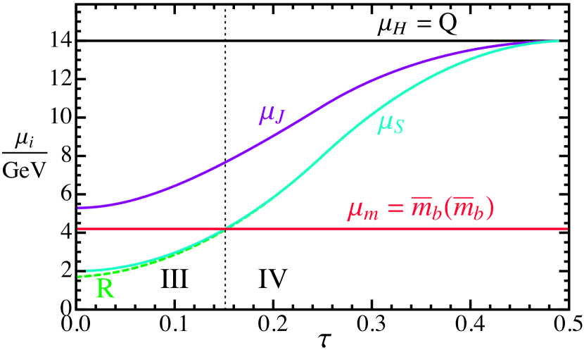
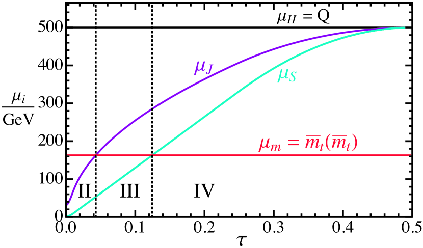
Refer to caption
Figure 10: Default profiles for Q=14𝑄14Q=14 GeV. The transition value for τ𝜏\tau between the scenarios III and IV is indicated by the dotted line.
Refer to caption
Figure 11: Default profiles for Q=500𝑄500Q=500 GeV. The transition values for τ𝜏\tau between the scenarios II and III and between the scenarios III and IV are indicated by dotted lines.

An important aspect of the practical implementation of the VFNS concerns the prescription how the predictions within the various scenarios discussed in the previous sections are patched together to obtain the complete spectrum of the thrust distribution. As described in Sec. III, one switches between neighboring scenarios when the mass scale is close to one of the kinematic scales related to the hard coefficient and the jet and the soft functions. It is therefore natural to tie the prescription for the transition to the τ𝜏\tau-dependent profile functions for μmsubscript𝜇𝑚\mu_{m}, μHsubscript𝜇𝐻\mu_{H}, μJsubscript𝜇𝐽\mu_{J} and μSsubscript𝜇𝑆\mu_{S}. In Figs. 10 and 11 the default profile functions (including the subtraction scale R𝑅R) are shown for Q=14𝑄14Q=14 GeV with μm=m¯b(m¯b)subscript𝜇𝑚subscript¯𝑚𝑏subscript¯𝑚𝑏\mu_{m}=\overline{m}_{b}(\overline{m}_{b}) and Q=500𝑄500Q=500 GeV with μm=m¯t(m¯t)subscript𝜇𝑚subscript¯𝑚𝑡subscript¯𝑚𝑡\mu_{m}=\overline{m}_{t}(\overline{m}_{t}), respectively. The prescription we adopt is that the transition concerning the scenarios II, III and IV is carried out when μmsubscript𝜇𝑚\mu_{m} is equal to μJsubscript𝜇𝐽\mu_{J} or μSsubscript𝜇𝑆\mu_{S}, respectively. For each choice of the profile functions and the mass mode matching scale this leads to a unique value of τ𝜏\tau for the transition. The resulting τ𝜏\tau regions for the scenarios II, III and IV are indicated in Figs. 10 and 11 by the black dotted vertical lines. We note that the general freedom to choose the transition value for τ𝜏\tau in some range causes variations in the predictions that are related to higher order corrections in the same way as changes of the renormalization and matching scales μmsubscript𝜇𝑚\mu_{m}, μHsubscript𝜇𝐻\mu_{H}, μJsubscript𝜇𝐽\mu_{J} and μSsubscript𝜇𝑆\mu_{S} in their respective ranges. Our prescription ties the choices made for their profile functions to the range in τ𝜏\tau of the scenarios.

The practical implementation of the factorization theorems from the different scenarios at N3LL involves a treatment of perturbative terms at higher orders that arise from cross terms of the perturbative series for the hard, jet and soft functions and the mass mode threshold factors. As mentioned above, we use the common approach to expand out the perturbative terms in the matrix elements and matching factors to 𝒪(αs2)𝒪superscriptsubscript𝛼𝑠2\mathcal{O}(\alpha_{s}^{2}), but to keep the RG evolution factors multiplying all expanded terms to the highest order. This approach has been proven advantageous to avoid spurious higher order corrections in the fixed-order expansion and to obtain reliable information on the remaining renormalization scale dependence at the corresponding order. This approach is also crucial to achieving a good numerical agreement of the factorization theorems in overlap regions where two different scenarios can be employed. In the same spirit, to avoid gaps at the transition points between neighboring scenarios related to spurious higher order terms and to obtain a continuous distribution, we also adopt the approach to expand in the series (at the scale μmsubscript𝜇𝑚\mu_{m}) for the decoupling relations of the strong coupling and the gap parameter Δ¯¯Δ\bar{\Delta} up to 𝒪(αs2)𝒪superscriptsubscript𝛼𝑠2\mathcal{O}(\alpha_{s}^{2}), see Eqs. (V.1) and (III.5).

Refer to caption
Figure 12: The thrust distribution at Q=14𝑄14Q=14 GeV including secondary massive bottom effects (blue, solid) compared to keeping the bottom quark massless (red, dashed).
Refer to caption
Figure 13: Relative secondary massive bottom effects for Q=14𝑄14Q=14 GeV (blue, solid), Q=35𝑄35Q=35 GeV (red, dashed) and Q=mZ𝑄subscript𝑚𝑍Q=m_{Z} (green, dotted).

In Fig. 12 the thrust distribution (for primary production of the four light quark flavors and secondary production of the light flavors and the bottom quark) normalized to the Born cross section σ0subscript𝜎0\sigma_{0} is shown for Q=14𝑄14Q=14 GeV at N3LL order, based on the factorization theorems for secondary massive bottom quarks with μm=m¯b(m¯b)subscript𝜇𝑚subscript¯𝑚𝑏subscript¯𝑚𝑏\mu_{m}=\overline{m}_{b}(\overline{m}_{b}) (blue, solid line) and in the massless approximation (red, dashed line). We see that the finite bottom mass effects are significant at and below the peak, but small in the tail region. Overall the secondary quark mass effects lead to a significant decrease in the peak cross section. Interestingly at the peak the deviations are only weakly depending on the value of Q𝑄Q. This is illustrated in Fig. 13, where we display for Q=14𝑄14Q=14 GeV (blue, solid curve), Q=35𝑄35Q=35 GeV (red, dashed curve) and Q=mZ𝑄subscript𝑚𝑍Q=m_{Z} (green, dotted curve) the relative change due to the finite mass of the secondary massive bottom quarks Δσ(mb)Δ𝜎subscript𝑚𝑏\Delta\sigma(m_{b}), with

Δσ(m)dσdτ(m)dσdτ(m=0)dσdτ(m=0).Δ𝜎𝑚d𝜎d𝜏𝑚d𝜎d𝜏𝑚0d𝜎d𝜏𝑚0\displaystyle\Delta\sigma(m)\,\equiv\,\frac{\frac{\mathrm{d}\sigma}{\mathrm{d}\tau}(m)-\frac{\mathrm{d}\sigma}{\mathrm{d}\tau}(m=0)}{\frac{\mathrm{d}\sigma}{\mathrm{d}\tau}(m=0)}\,. (166)

Here dσdτ(m)d𝜎d𝜏𝑚\frac{\mathrm{d}\sigma}{\mathrm{d}\tau}(m) is the complete thrust distribution at N3LL for primary massless quarks and for secondary quark production which includes the proper number of light quarks and an additional flavor with mass m𝑚m. We see that in the peak region ΔσΔ𝜎\Delta\sigma is up to 5%similar-toabsentpercent5\sim-5\% and depends only weakly on the Q𝑄Q value. In the tail region the mass effects from secondary bottom quarks amount to relative corrections below 1%percent11\% for Q=14𝑄14Q=14 GeV, and they quickly decrease for larger values of Q𝑄Q.

Refer to caption
Figure 14: Dependence of ΔσΔ𝜎\Delta\sigma on the mass mode matching scale μmsubscript𝜇𝑚\mu_{m} for secondary bottom quarks for Q=14𝑄14Q=14 GeV: μm=mbsubscript𝜇𝑚subscript𝑚𝑏\mu_{m}=m_{b} (blue, solid), μm=mb/2subscript𝜇𝑚subscript𝑚𝑏2\mu_{m}=m_{b}/2 (red, dashed), μm=2mbsubscript𝜇𝑚2subscript𝑚𝑏\mu_{m}=2m_{b} (green, dotted).

It is also important to discuss the scale variations of the mass correction ΔσΔ𝜎\Delta\sigma. In Fig. 14 the impact of the variations of μmsubscript𝜇𝑚\mu_{m} is illustrated for the bottom quark case for Q=14𝑄14Q=14 GeV. The curves are for μmsubscript𝜇𝑚\mu_{m} equal to the MS¯¯MS\overline{\rm MS} bottom mass and for variations by factors of two and one half. The μmsubscript𝜇𝑚\mu_{m} dependence is quite small in the tail and far-tail regions. In the peak region, on the other hand, the variation of ΔσΔ𝜎\Delta\sigma increases to 4%percent44\% and grows even further below the peak, where ΔσΔ𝜎\Delta\sigma changes sign. This behavior is generic for the bottom quark case and very similar for other values of Q𝑄Q. This behavior might appear formidable for ΔσΔ𝜎\Delta\sigma, but it should be judged taking into account that in the peak region the dependence on μmsubscript𝜇𝑚\mu_{m} is related to missing higher order corrections of the complete thrust distribution and not only to ΔσΔ𝜎\Delta\sigma. In other words, the finite mass of the secondary heavy quark leads to a modification of the peak behavior which represents a property of the complete thrust distribution and not just of ΔσΔ𝜎\Delta\sigma itself. The result shows that variations of μmsubscript𝜇𝑚\mu_{m} need to be accounted for when estimating perturbative uncertainties in the peak region.
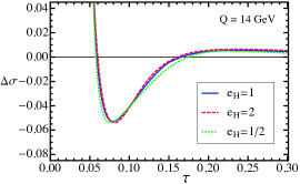
Refer to caption
Refer to caption
Refer to caption
Refer to caption
Refer to caption
Figure 15: Relative secondary bottom mass effects for Q=14𝑄14Q=14 GeV under variation of the profile parameters for the hard, jet and soft scales.

In this context it is also important to examine the variation of ΔσΔ𝜎\Delta\sigma due to changes of the profile functions for μHsubscript𝜇𝐻\mu_{H}, μJsubscript𝜇𝐽\mu_{J}, μSsubscript𝜇𝑆\mu_{S} as well as for R𝑅R. In Fig. 15 ΔσΔ𝜎\Delta\sigma is shown for the bottom quark case at Q=14𝑄14Q=14 GeV for variations of the parameters eHsubscript𝑒𝐻e_{H}, eJsubscript𝑒𝐽e_{J}, μ0subscript𝜇0\mu_{0}, n1subscript𝑛1n_{1} and t2subscript𝑡2t_{2}, see Eqs. (151)-(159), which parametrize changes of the profile functions. The ranges of variation are described in the figure caption and are identical to the ones used for the thrust analysis of Ref. Abbate:2010xh (except for n1subscript𝑛1n_{1} which requires a lower range for low Q𝑄Q values). These variations induce visible changes in ΔσΔ𝜎\Delta\sigma, but they are in general much smaller than the dependence on μmsubscript𝜇𝑚\mu_{m} discussed just above. This outcome is again generic for other values of Q𝑄Q and also for the top quark case and shows that independent variations of the profile functions and of μmsubscript𝜇𝑚\mu_{m} are essential for a thorough assessment of the scale variations of the complete thrust distribution.

We complete our analysis by showing in Fig. 16 the thrust distribution for primary light quark production at Q=500𝑄500Q=500 GeV with nl=5subscript𝑛𝑙5n_{l}=5 massless flavors and a secondary massive top quark (blue, solid line). The figure also shows the prediction for the case where the secondary top quark is treated as massless (red, dashed line). For all parameters the default values mentioned above are used. It is visible that the finite top quark mass causes, besides a reduction of the distribution at the peak, as we have observed in the bottom quark case, also a shift of the peak to lower τ𝜏\tau values. This effect is related to the top quark mass effects in the R-scale dependence of the gap parameter, which is significantly modified below the massive threshold as described in Sec. III.5. In Fig. 17 ΔσΔ𝜎\Delta\sigma is shown for the top quark case for Q=500𝑄500Q=500 GeV (blue, solid line), Q=1000𝑄1000Q=1000 GeV (red, dashed line) and Q=3000𝑄3000Q=3000 GeV (green, dotted line). We find again sizable mass effects at and below the peak of the distribution. In the tail region, on the other hand, the top mass effects are relatively small. At the peak the mass effects amount to 1020%10percent2010-20\% and remain significant even for large values of Q𝑄Q. In contrast to the bottom quark case, the size of the top mass effects is larger than the variations due to changes of the mass mode matching scale μmsubscript𝜇𝑚\mu_{m} which amount to 111 to 2%percent22\% in the total cross section. We note that in the top quark case and for these c.m. energies the decoupling limit, i.e. the thrust distribution with just 5 massless flavors and a decoupled top quark, is at the peak much closer to the VFNS prediction than the massless top approximation (shown in the red dashed curve). This is because in the peak region the top mass is significantly larger than the jet and the soft scales such that the decoupling approximation is more appropriate than the massless one.

VII Conclusions

In this work we have provided a variable flavor number scheme (VFNS) for inclusive final state jets taking the production of secondary massive quarks (see Fig. 1) for the thrust distribution as the concrete application. In the dijet limit the singular terms factorize into a hard function given by a Wilson coefficient for the dijet production current, a jet function describing the hard collinear radiation within the jet and a soft function describing soft radiation between the jets. The factorization is based on the fact that the typical invariant masses of the fluctuations described by these factors are widely separated, where the size of these scales depends on the thrust variable τ𝜏\tau.

Including the radiation of secondary massive quarks the situation becomes more complicated since the quark mass adds another τ𝜏\tau-independent scale to the situation that can lead to different kinds of hierarchies or relations w.r. to the hard jet and soft scales. Apart from a more complicated analytic structure one has to deal with potential mass singularities and the summation of logarithms of the mass – all with the requirement that the massive quark decouples in the infinite mass limit and that one obtains the well-known massless quark description in the limit that the quark mass vanishes.
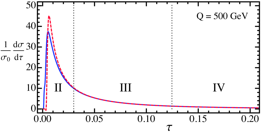
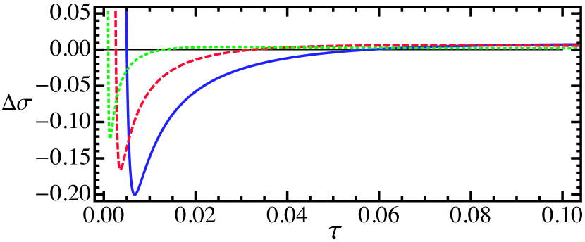
Refer to caption
Figure 16: The thrust distribution at Q=500𝑄500Q=500 GeV including secondary massive top effects (blue, solid) compared to keeping the top quark massless (red, dashed).
Refer to caption
Figure 17: Relative secondary massive top effects for Q=500𝑄500Q=500 GeV (blue, solid), Q=1000𝑄1000Q=1000 GeV (red, dashed) and Q=3000𝑄3000Q=3000 GeV (green, dotted).

The VFNS we provide is based on the hierarchy between the hard, jet and soft scales and accounts in addition for the quark mass, for which, however, no assumption concerning a hierarchy w.r. to the other scales has to be imposed. The effective theory description was explained in detail in Ref. Gritschacher:2013pha using the field theoretic analogy between secondary massive quarks and the radiation of “massive gluons”. The four emerging effective theories are related to the four hierarchical regions of the mass w.r. to the hard, jet and soft scales, and deal with collinear and soft massless quarks and gluons as well as corresponding “mass modes”. The treatment of these mass modes differs for each of the four effective theories and leads to modifications of the known factorization for massless quarks. These (i) add a quark mass dependence in the hard coefficient, the jet and soft functions, (ii) affect the RG evolution which is carried out with different flavor numbers above and below the quark mass scale and (iii) lead to additional massive threshold correction factors when the RG evolution of one of the structures crosses the mass scale. The factorization scale where this crossover is performed (“mass mode matching scale”) can be varied in analogy to the renormalization scales. An essential aspect of the VFNS is that in a transition region between two neighboring effective theories both of their descriptions can be used which ensures that the transition is continuous (up to perturbative terms from beyond the order that is employed in the description).

An important outcome of our mass mode treatment is that the way in which the massive quark contributes to the hard coefficient, the jet function and the soft function as well as to their mass mode threshold factors can be determined for each of them individually without having to deal with the factorization theorem for the thrust distribution as a whole. This is related to the fact that the hard coefficient, the jet function and the soft function are by themselves well-defined field theoretical quantities that can be renormalized consistently. If the description includes the small mass case (including the massless limit) the MS¯¯MS\overline{\rm MS} renormalization prescription is employed for the secondary massive quark corrections. On the other hand, if the description includes the large mass case (including the decoupling limit) the on-shell (low momentum-subtraction) renormalization condition is employed for the secondary massive quark corrections. For sufficiently large scales hierarchies it may be possible to use massless quark results with the appropriate number of flavors for some of the structures as a good approximation. The transition regions are located where the quark mass is of the order of the hard, jet or soft scales, and the difference of the renormalized quantities constitutes the mass mode threshold correction factors.

We have discussed the numerical impact of the secondary quark mass effects on the thrust distribution. These turn out to be small corrections in the tail region, but sizable at the peak, so that a phenomenological analysis of this region will have to take them into account. For the assessment of the renormalization scale dependence it is crucial to account for changes of the mass mode matching scale.

In this work we have demonstrated the concept of a VFNS for final state jets for the secondary massive quark effects in the thrust distribution. In subsequent publications our proposed VFNS shall be applied also to the primary production of massive quarks Butenschoen:2014 , where new subtleties arise as well as to other processes including deep inelastic scattering Hoang:2015iva , where the relation to VFNS for initial state massive quarks is elucidated.

Acknowledgements.
We thank the Erwin-Schrödinger Institute (ESI) for partial support in the framework of the ESI program “Jets and Quantum Fields for LHC and Future Colliders”. We thank Daniel Samitz for pointing out an error in Eq. (167) in the previous version of this paper. P. P. would like to thank Bahman Dehnadi for helpful discussions and cross checks in parts of the numerical analysis.

Note added: After initial submission we received Ref. Ablinger:2014vwa where the 𝒪(αs3)𝒪superscriptsubscript𝛼𝑠3\mathcal{O}(\alpha_{s}^{3}) non-singlet corrections to the heavy flavor matching of the parton distribution functions were calculated. Considerations in DIS for large x𝑥x in analogy to this work Hoang:2014ira ; Hoang:2015iva lead to a consistency relation similar to Eq. (V.4) involving this threshold correction, which implies

3C,+=143J,+=143S,+subscriptsuperscript𝐶314subscriptsuperscript𝐽314subscriptsuperscript𝑆3\displaystyle\mathcal{M}^{C,+}_{3}=\frac{1}{4}\mathcal{M}^{J,+}_{3}=\frac{1}{4}\mathcal{M}^{S,+}_{3} (167)
=CFTF{CF(1417276049ζ3+8π415323B4)\displaystyle=-C_{\!F}T_{F}\left\{C_{\!F}\!\left(\frac{1417}{27}-\frac{604}{9}\,\zeta_{3}+\frac{8\pi^{4}}{15}-\frac{32}{3}B_{4}\!\right)\right.
+CA(17726729+824π2243+30ζ388π4135+163B4)subscript𝐶𝐴17726729824superscript𝜋224330subscript𝜁388superscript𝜋4135163subscript𝐵4\displaystyle+C_{\!A}\!\left(\!-\,\frac{17726}{729}+\frac{824\pi^{2}}{243}+30\,\zeta_{3}-\frac{88\pi^{4}}{135}+\frac{16}{3}B_{4}\!\right)
+TFnl(12032729+25627ζ3)+TF(603272944827ζ3)},\displaystyle+\left.T_{F}n_{l}\!\left(\!-\,\frac{12032}{729}+\frac{256}{27}\,\zeta_{3}\!\right)+T_{F}\!\left(\frac{6032}{729}-\frac{448}{27}\,\zeta_{3}\!\right)\!\right\},

where

B4=23ln4(2)2π23ln2(2)13π4180+16Li4(12).subscript𝐵423superscriptln422superscript𝜋23superscriptln2213superscript𝜋418016subscriptLi412\displaystyle\!\!\!B_{4}=\frac{2}{3}\,\textrm{ln}^{4}(2)-\frac{2\pi^{2}}{3}\,\textrm{ln}^{2}(2)-\frac{13\pi^{4}}{180}+16\,\textrm{Li}_{4}\Big{(}\frac{1}{2}\Big{)}\,. (168)

For nl=4subscript𝑛𝑙4n_{l}=4 and nl=5subscript𝑛𝑙5n_{l}=5 light flavors one obtains the numerical values 3C,+=28.2337subscriptsuperscript𝐶328.2337\mathcal{M}^{C,+}_{3}=28.2337 and 3C,+=29.9362subscriptsuperscript𝐶329.9362\mathcal{M}^{C,+}_{3}=29.9362, respectively.222222Note that the published version of this paper contains an error in Eq. (167) and the associated numerical values. We note that the numerical impact of the constants 3C,+subscriptsuperscript𝐶3\mathcal{M}^{C,+}_{3} and 3J,+subscriptsuperscript𝐽3\mathcal{M}^{J,+}_{3} in the analysis of Sec. VI is negligibly small.

Appendix A Plus-distributions

We give the definition and integral prescription for the plus-distributions appearing in the nonlocal evolution factors, denoted by [lnn(x)/x1+ω]+subscriptdelimited-[]superscriptln𝑛𝑥superscript𝑥1𝜔[\textrm{ln}^{n}(x)/x^{1+\omega}]_{+}, for arbitrary (non-vanishing) ω𝜔\omega. The prescription of these plus-distributions is based on an analytic continuation to a domain with a well-behaved convergence following Ref. Fleming:2007xt

[θ(x)lnn(x)x1+ω]+ω<0superscript𝜔0subscriptdelimited-[]𝜃𝑥superscriptln𝑛𝑥superscript𝑥1𝜔absent\displaystyle\left[\frac{\theta(x)\textrm{ln}^{n}(x)}{x^{1+\omega}}\right]_{+}\stackrel{{\scriptstyle\omega<0}}{{\longrightarrow}} θ(x)lnn(x)x1+ω.𝜃𝑥superscriptln𝑛𝑥superscript𝑥1𝜔\displaystyle\,\,\,\frac{\theta(x)\,\textrm{ln}^{n}(x)}{x^{1+\omega}}\,. (169)

This leads to a definition based on the subtraction of strictly divergent terms at x=0𝑥0x=0 that can be generalized to arbitrary values of ω𝜔\omega in a straightforward way:

[θ(x)lnn(x)x1+ω]+=limϵ0[θ(xϵ)lnn(x)x1+ωk=0δ(k)(x)(1)kk!Γ(n+1,(ωk)ln(ϵ))(ωk)n+1].subscriptdelimited-[]𝜃𝑥superscriptln𝑛𝑥superscript𝑥1𝜔subscriptitalic-ϵ0delimited-[]𝜃𝑥italic-ϵsuperscriptln𝑛𝑥superscript𝑥1𝜔superscriptsubscript𝑘0superscript𝛿𝑘𝑥superscript1𝑘𝑘Γ𝑛1𝜔𝑘lnitalic-ϵsuperscript𝜔𝑘𝑛1\displaystyle\left[\frac{\theta(x)\textrm{ln}^{n}(x)}{x^{1+\omega}}\right]_{+}=\lim_{\epsilon\rightarrow 0}\left[\frac{\theta(x-\epsilon)\textrm{ln}^{n}(x)}{x^{1+\omega}}-\sum_{k=0}^{\infty}\delta^{(k)}(x)\,\frac{(-1)^{k}}{k!}\,\frac{\Gamma(n+1,(\omega-k)\textrm{ln}(\epsilon))}{(\omega-k)^{n+1}}\right]\,. (170)

This expression can be rewritten as an integral prescription

0Xdx[θ(x)lnnxx1+ω]+f(x)=0Xdxlnn(x)x1+ω[f(x)k=0f(k)(0)xkk!]k=0f(k)(0)1k!Γ(n+1,(ωk)ln(X))(ωk)n+1,superscriptsubscript0𝑋differential-d𝑥subscriptdelimited-[]𝜃𝑥superscriptln𝑛𝑥superscript𝑥1𝜔𝑓𝑥superscriptsubscript0𝑋differential-d𝑥superscriptln𝑛𝑥superscript𝑥1𝜔delimited-[]𝑓𝑥superscriptsubscript𝑘0superscript𝑓𝑘0superscript𝑥𝑘𝑘superscriptsubscript𝑘0superscript𝑓𝑘01𝑘Γ𝑛1𝜔𝑘ln𝑋superscript𝜔𝑘𝑛1\displaystyle\int_{0}^{X}\mathrm{d}x\left[\frac{\theta(x)\textrm{ln}^{n}x}{x^{1+\omega}}\right]_{+}f(x)=\int_{0}^{X}\mathrm{d}x\,\frac{\textrm{ln}^{n}(x)}{x^{1+\omega}}\left[f(x)-\sum_{k=0}^{\infty}f^{(k)}(0)\frac{x^{k}}{k!}\right]-\sum_{k=0}^{\infty}f^{(k)}(0)\frac{1}{k!}\frac{\Gamma(n+1,(\omega-k)\textrm{ln}(X))}{(\omega-k)^{n+1}}\,, (171)

where the sums can be truncated for k=N𝑘𝑁k=N if ω<N+1𝜔𝑁1\omega<N+1.

References

  • (1) A. Juste, S. Mantry, A. Mitov, A. Penin, P. Skands, et al., Determination of the top quark mass circa 2013: methods, subtleties, perspectives, arXiv:1310.0799, (2013).
  • (2) A. Jung, M. Schulze, and J. Shelton, Kinematics of Top Quark Final States: A Snowmass White Paper, arXiv:1309.2889, (2013).
  • (3) K. Agashe et al., Snowmass 2013 Top quark working group report, arXiv:1311.2028, (2013).
  • (4) S. Alekhin, J. Blümlein, K. Daum, K. Lipka, and S. Moch, Precise charm-quark mass from deep-inelastic scattering, Phys.Lett. B720, 172–176 (2013).
  • (5) H. Abramowicz et al., Combination and QCD Analysis of Charm Production Cross Section Measurements in Deep-Inelastic ep Scattering at HERA, Eur.Phys.J. C73, 2311 (2013).
  • (6) K. Kovarik, T. Stavreva, A. Kusina, T. Jezo, F. Olness, et al., A Survey of Heavy Quark Theory for PDF Analyses, Nucl.Phys.Proc.Suppl. 222-224, 52–60 (2012).
  • (7) J. Campbell, K. Hatakeyama, J. Huston, F. Petriello, J. R. Andersen, et al., Report of the Snowmass 2013 energy frontier QCD working group, arXiv:1310.5189, (2013).
  • (8) M. Aivazis, J. C. Collins, F. I. Olness, and W.-K. Tung, Leptoproduction of heavy quarks. 2. A Unified QCD formulation of charged and neutral current processes from fixed target to collider energies, Phys. Rev. D50, 3102–3118 (1994).
  • (9) M. Aivazis, F. I. Olness, and W.-K. Tung, Leptoproduction of heavy quarks. 1. General formalism and kinematics of charged current and neutral current production processes, Phys. Rev. D50, 3085–3101 (1994).
  • (10) C. W. Bauer, S. Fleming, and M. E. Luke, Summing Sudakov logarithms in BXsγ𝐵subscript𝑋𝑠𝛾B\to X_{s}\gamma in effective field theory, Phys. Rev. D63, 014006 (2000).
  • (11) C. W. Bauer, S. Fleming, D. Pirjol, and I. W. Stewart, An Effective field theory for collinear and soft gluons: Heavy to light decays, Phys. Rev. D63, 114020 (2001).
  • (12) I. W. Stewart, F. J. Tackmann, and W. J. Waalewijn, N-Jettiness: An Inclusive Event Shape to Veto Jets, Phys. Rev. Lett. 105, 092002 (2010).
  • (13) A. H. Hoang and I. W. Stewart, Designing gapped soft functions for jet production, Phys. Lett. B660, 483–493 (2008).
  • (14) V. Mateu, I. W. Stewart, and J. Thaler, Power Corrections to Event Shapes with Mass-Dependent Operators, Phys. Rev. D87, 014025 (2013).
  • (15) S. Gritschacher, A. Hoang, I. Jemos, and P. Pietrulewicz, Secondary Heavy Quark Production in Jets through Mass Modes, Phys. Rev. D88, 034021 (2013).
  • (16) S. Gritschacher, A. Hoang, I. Jemos, and P. Pietrulewicz, Two loop soft function for secondary massive quarks, Phys. Rev. D89, 014035 (2014).
  • (17) R. Abbate, M. Fickinger, A. H. Hoang, V. Mateu, and I. W. Stewart, Thrust at N3LL with Power Corrections and a Precision Global Fit for αs(mZ)subscript𝛼𝑠subscript𝑚𝑍\alpha_{s}(m_{Z}), Phys. Rev. D83, 074021 (2011).
  • (18) A. H. Hoang and S. Kluth, Hemisphere Soft Function at 𝒪(αs2)𝒪superscriptsubscript𝛼𝑠2\mathcal{O}(\alpha_{s}^{2}) for Dijet Production in e+esuperscript𝑒superscript𝑒e^{+}\,e^{-} Annihilation, arXiv:0806.3852, (2008).
  • (19) G. P. Korchemsky and G. F. Sterman, Power corrections to event shapes and factorization, Nucl. Phys. B555, 335–351 (1999).
  • (20) M. D. Schwartz, Resummation and NLO matching of event shapes with effective field theory, Phys. Rev. D77, 014026 (2008).
  • (21) S. Fleming, A. H. Hoang, S. Mantry, and I. W. Stewart, Jets from massive unstable particles: Top-mass determination, Phys. Rev. D77, 074010 (2008).
  • (22) T. Matsuura and W. van Neerven, Second Order Logarithmic Corrections to the Drell-Yan Cross-section, Z.Phys. C38, 623 (1988).
  • (23) T. Becher and M. Neubert, Toward a NNLO calculation of the B¯Xsγ¯𝐵subscript𝑋𝑠𝛾\bar{B}\to X_{s}\gamma decay rate with a cut on photon energy. II. Two-loop result for the jet function, Phys. Lett. B637, 251–259 (2006).
  • (24) R. Kelley, M. D. Schwartz, R. M. Schabinger, and H. X. Zhu, The two-loop hemisphere soft function, Phys. Rev. D84, 045022 (2011).
  • (25) P. F. Monni, T. Gehrmann, and G. Luisoni, Two-Loop Soft Corrections and Resummation of the Thrust Distribution in the Dijet Region, JHEP 1108, 010 (2011).
  • (26) A. H. Hoang, A. Jain, I. Scimemi, and I. W. Stewart, Infrared Renormalization Group Flow for Heavy Quark Masses, Phys.Rev.Lett. 101, 151602 (2008).
  • (27) A. H. Hoang, A. Jain, I. Scimemi, and I. W. Stewart, R-evolution: Improving perturbative QCD, Phys.Rev. D82, 011501 (2010).
  • (28) A. K. Leibovich, Z. Ligeti, and M. B. Wise, Comment on quark masses in SCET, Phys. Lett. B564, 231–234 (2003).
  • (29) J.-Y. Chiu, A. Fuhrer, A. H. Hoang, R. Kelley, and A. V. Manohar, Soft-Collinear Factorization and Zero-Bin Subtractions, Phys. Rev. D79, 053007 (2009).
  • (30) B. A. Kniehl, Two Loop QED Vertex Correction From Virtual Heavy Fermions, Phys.Lett. B237, 127 (1990).
  • (31) A. Hoang, Applications of two loop calculations in the standard model and its minimal supersymmetric extension, (1995).
  • (32) T. Becher and G. Bell, Analytic Regularization in Soft-Collinear Effective Theory, Phys. Lett. B713, 41–46 (2012).
  • (33) J.-Y. Chiu, A. Jain, D. Neill, and I. Z. Rothstein, A Formalism for the Systematic Treatment of Rapidity Logarithms in Quantum Field Theory, JHEP 1205, 084 (2012).
  • (34) J.-Y. Chiu, A. Jain, D. Neill, and I. Z. Rothstein, The Rapidity Renormalization Group, Phys.Rev.Lett. 108, 151601 (2012).
  • (35) A. H. Hoang, A. Pathak, P. Pietrulewicz, and I. W. Stewart, Hard Matching for Boosted Tops at Two Loops, JHEP 12, 059 (2015).
  • (36) R. Abbate, M. Fickinger, A. H. Hoang, V. Mateu, and I. W. Stewart, Precision Thrust Cumulant Moments at N3superscript𝑁3N^{3}LL, Phys.Rev. D86, 094002 (2012).
  • (37) S. Gritschacher, Massive gluon effects in event shape distributions, diploma thesis, (2011).
  • (38) M. Butenschön, B. Dehnadi, A. H. Hoang, V. Mateu, and I. W. Stewart, in preparation.
  • (39) A. H. Hoang, P. Pietrulewicz, and D. Samitz, Variable Flavor Number Scheme for Final State Jets in DIS, arXiv:1508.04323, (2015).
  • (40) J. Ablinger, A. Behring, J. Blümlein, A. De Freitas, A. Hasselhuhn, et al., The 3-Loop Non-Singlet Heavy Flavor Contributions and Anomalous Dimensions for the Structure Function F2(x,Q2)subscript𝐹2𝑥superscript𝑄2F_{2}(x,Q^{2}) and Transversity, Nucl. Phys. B886, 733–823 (2014).
  • (41) A. H. Hoang, P. Pietrulewicz, and D. Samitz, Variable Flavor Number Scheme for Final State Jets, arXiv:1406.5885, (2014).
  • (42) S. Fleming, A. H. Hoang, S. Mantry, and I. W. Stewart, Top Jets in the Peak Region: Factorization Analysis with NLL Resummation, Phys. Rev. D77, 114003 (2008).