.

NORDITA-2014-61
UUITP-04/14

Classical and quantum temperature fluctuations via holography

Alexander Balatsky^1,2, Sven Bjarke Gudnason¹, Yaron Kedem¹, Alexander Krikun^1,3,
Lárus Thorlacius^1,4,5 and Konstantin Zarembo^1,3,6

¹Nordita, KTH Royal Institute of Technology and Stockholm University, Roslagstullsbacken 23, SE-106 91 Stockholm, Sweden
²Institute for Materials Science, Los Alamos National Laboratory, Los Alamos, NM 87545, USA
³Institute of Theoretical and Experimental Physics, B. Cheremushkinskaya 25, 117218 Moscow, Russia
⁴University of Iceland, Science Institute, Dunhaga 3, IS-107 Reykjavik, Iceland
⁵ The Oskar Klein Centre for Cosmoparticle Physics, Department of Physics, Stockholm University, AlbaNova University Centre, 10691 Stockholm, Sweden
⁶Department of Physics and Astronomy, Uppsala University SE-751 08 Uppsala, Sweden

Abstract

We study local temperature fluctuations in a 2+1 dimensional CFT on the sphere, dual to a black hole in asymptotically AdS spacetime. The fluctuation spectrum is governed by the lowest-lying hydrodynamic modes of the system whose frequency and damping rate determine whether temperature fluctuations are thermal or quantum. We calculate numerically the corresponding quasinormal frequencies and match the result with the hydrodynamics of the dual CFT at large temperature. As a by-product of our analysis we determine the appropriate boundary conditions for calculating low-lying quasinormal modes for a four-dimensional Reissner-Nordström black hole in global AdS.

1 Introduction

The field of black hole thermodynamics was cast into life by the definition of black hole entropy and temperature in the seminal papers by Bekenstein [1] and Hawking [2]. Early on it was viewed as an interesting analogy between dynamical equations of two rather different fields of physics, general relativity and statistical mechanics, but with the advent of anti de Sitter - conformal field theory (AdS/CFT) duality [3] the analogy has been promoted to a precise correspondence for a class of black holes.

A Schwarzschild black hole in asymptotically flat spacetime is unstable due to the Hawking effect. It evaporates if it is surrounded by empty spacetime and as it has negative heat capacity it cannot be in stable equilibrium with a thermal gas either. In fact, due to the Jeans instability, the thermodynamic limit is not well defined in Einstein gravity in asymptotically flat spacetime and there exist no equilibrium configurations at finite temperature and density.

The situation is different in asymptotically AdS spacetime, where a large black hole above the Hawking-Page phase transition [4] is a stable configuration. Under AdS/CFT duality, such a black hole corresponds to a thermal state in the conformal field theory at the boundary of spacetime, with the CFT temperature equal to the Hawking temperature of the black hole [5]. The appropriate interpretation of black hole thermodynamics in asymptotically AdS spacetime is in terms of the dual field theory rather than spacetime physics in the bulk. The AdS black hole geometry itself is a solution of the classical field equations of general relativity without matter and observers in free fall outside a large AdS black hole do not detect any propagating Hawking radiation [6]. Nonetheless the Hawking temperature, interpreted as the temperature of the dual CFT, is a well-defined observable.

Any macroscopic physical observable is subject to statistical fluctuations. When one measures a particular quantity one gets results which are distributed around the mean value with some finite standard deviation. For macroscopic objects the fluctuations are usually governed by random thermal noise, but when the system is small enough, the quantum uncertainty principle starts playing a significant role and changes the overall behavior of the system [7]. Thus one distinguishes between the regimes of thermal and quantum fluctuations of the observable. This treatment can readily be applied to fluctuations in the temperature of the system. Due to energy conservation, the mean value of the temperature in the dual field theory does not fluctuate with time. However, local temperature fluctuations do exist and they will exhibit thermal or quantum behavior depending on system parameters.

In this paper we use the AdS/CFT duality to investigate local temperature fluctuations in a field-theoretic system at strong coupling via the dynamics of asymptotically AdS black holes. We focus on the AdS-Reissner-Nordström solution dual to a CFT at finite temperature and chemical potential. The rationale for switching on a chemical potential is that it allows us to consider low temperature without compromising thermodynamic stability, which as we shall see leads to a crossover from a thermal to a quantum regime in temperature fluctuations.

The paper is organized as follows. In Section 2 we recall the notion of temperature fluctuations and analyze them in the case of overdamped and underdamped modes. In Section 3 we set up the problem of calculating local temperature fluctuations of the CFT in compact space. Sections 4 and 5 consider the hydrodynamic approximation to the sound and diffusive modes of the CFT on a sphere, dual to the black hole under consideration, in case of zero and finite chemical potential, respectively. In Section 6 we carry out a direct gravitational analysis of the system and compute numerically the lowest-lying quasinormal modes of the black hole. We conclude in Section 7. Appendix A is devoted to a detailed analysis of the transition between classical and quantum regimes of the fluctuations. Appendix B collects various thermodynamic relations, that we use throughout the paper. In Appendix C we consider details of the calculation of QNMs of the Reissner-Nordström black hole in global AdS₄.

2 Temperature fluctuations

Temperature fluctuations in classical systems have been widely studied. In classical statistical mechanics the variance of a statistical variable is given by the width of its probability distribution, which for temperature gives [8]

$$\langle\delta T^{2}\rangle=\frac{T^{2}}{C_{v}},$$ (1)

where $T$ is the temperature and $C_{v}$ is the heat capacity. From this expression, it is clear that in order for the temperature to be a well-defined quantity, the heat capacity must be large.

Temperature fluctuations close to equilibrium can be described by linear response theory [9, 7]. To this end, we consider a system in which the temperature of a black body is in equilibrium with the surrounding radiation. In response to an external perturbation, the system will relax to equilibrium on a characteristic time-scale $\tau$, with its temperature changing with time according to

$$\frac{dT}{dt}=-\frac{T-T_{e}}{\tau},$$ (2)

with $T_{e}$ being the equilibrium temperature. The change in entropy $\Delta S$ caused by a perturbation is related to the change in temperature as

$$\Delta T_{e}=\frac{\partial T}{\partial S}\Delta S=\frac{T}{C_{v}}\Delta S.$$ (3)

The Fourier spectrum of temperature fluctuations is thus related to that of the entropy by a response function (generalized susceptibility):

$$\delta T(\omega)=\alpha(\omega)\Delta S(\omega),$$ (4)

given by (3) and (2):

$$\alpha(\omega)=\frac{T}{C_{v}}\frac{1}{1-i\omega\tau}\,.$$ (5)

The fluctuation-dissipation theorem [8] relates the mean-square temperature fluctuation to the imaginary part of the susceptibility:

$$\langle\delta T^{2}\rangle=\hbar\int_{-\infty}^{\infty}\frac{d\omega}{2\pi}\,\,\mathop{\rm Im}\alpha(\omega)\coth\frac{\hbar\omega}{2T}.$$ (6)

The divergence of the integral at high frequencies is fictitious, and is an artifact of the single-pole form for the response function, which is just an approximation valid at low frequencies. The integral cannot be carried out exactly, but it can easily be approximated in various limits [7]. In particular the classical result (1) is reproduced at $T\tau\gg\hbar$, by replacing the $\coth$ by the inverse of its argument. In the opposite regime of $T\tau\ll\hbar$,

$$\langle\delta T^{2}\rangle\simeq\frac{\hbar T}{\pi C_{v}\tau}\,\ln\omega_{c}\tau,$$ (7)

where $\omega_{c}$ is a cutoff frequency, see App. A for details.

Thus far we have been working in the approximation in which the dominant relaxation is given by an overdamped mode. In studying temperature fluctuations of the AdS black hole we will encounter a different situation, when relaxation to equilibrium is driven by slowly decaying oscillations. The above discussion then needs to be modified. To this end, we consider the damped harmonic oscillator with an internal frequency $\Omega$ and relaxation rate $\Gamma$. The response function, or the retarded Green function, is given by

$$\alpha(\omega)=G^{R}(\omega)=-\frac{\Omega^{2}}{k}\frac{1}{\omega^{2}-\Omega^{2}+i2\omega\Gamma}.$$ (8)

Here $k$ is the “spring constant” which in our case is given by $k=\frac{C_{v}}{T}$ since the change in free energy is $\Delta S\delta T=\frac{C_{v}}{T}\delta T^{2}$. So the response function is given by

$$\alpha(\omega)=-\frac{T\Omega^{2}}{C_{v}}\frac{\omega^{2}-\Omega^{2}-i2\omega\Gamma}{(\omega^{2}-\Omega^{2})^{2}+4\omega^{2}\Gamma^{2}}.$$ (9)

The two oscillation poles in the complex frequency plane are located at

$$\omega =-i\Gamma\pm\sqrt{\Omega^{2}-\Gamma^{2}}\simeq-i\Gamma\pm\Omega.$$

The approximate equality on the right holds for $\Omega\gg\Gamma$, the case that we will encounter shortly in the holographic setup.

Depending on the ratios between the three parameters $T$, $\Omega$ and $\Gamma$, various regimes of temperature fluctuations are possible. When the temperature is much bigger than both the frequency and the decay rate, the classical result (1) is recovered. As may be expected, this result does not depend on a particular form of the response function, and actually follows on very general grounds from the Kramers-Kronig relation

$$\mathop{\mathrm{Re}}\alpha(\omega^{\prime})=-\!\!\!\!\!\!\int_{-\infty}^{+\infty}\frac{d\omega}{\pi}\,\,\frac{\mathop{\mathrm{Im}}\alpha(\omega)}{\omega-\omega^{\prime}}\,.$$ (10)

Indeed, setting $\omega^{\prime}=0$, and taking into account that

$$\mathop{\mathrm{Re}}\alpha(0)=\alpha(0)=\frac{T}{C_{v}}\,,$$ (11)

we get (1) from (6) whenever$\coth$ can be replaced by the inverse of its argument. The constraint (11) will be a useful consistency check on our holographic calculations of the response function. For the response function of the form (9), the leading quantum corrections can be readily computed, here for simplicity displayed in the oscillatory regime $T/\hbar\gg\Omega\gg\Gamma$ (see App. A):

$$\langle\delta T^{2}\rangle\simeq\frac{T^{2}}{C_{v}}+\frac{\hbar^{2}\Omega^{2}}{12C_{v}}-\frac{\hbar^{3}\zeta(3)\Omega^{2}\Gamma}{2\pi^{3}C_{v}T}+\mathcal{O}\left(\frac{\hbar^{4}\Omega^{2}\Gamma^{2}}{T^{2}}\right).$$ (12)

The first two terms come from the poles in the response function and the third term is due to a summation of Matsubara modes.

The “quantum” regime comes about when $T/\hbar\ll{\rm max}(\Omega,\Gamma)/2\pi$, which when $\Omega\gg\Gamma$ yields

$$\langle\delta T^{2}\rangle\simeq\frac{\hbar T\Omega}{2C_{v}}.$$ (13)

A careful analysis is carried out in App. A where we define the classicality parameter:

$$\mathfrak{q}\equiv\frac{2\pi T}{\hbar\sqrt{\Omega^{2}+\Gamma^{2}}}.$$ (14)

If $\mathfrak{q}>1$ the temperature fluctuations are in the classical regime, while for $\mathfrak{q}<1$ the temperature fluctuations are quantum.

The overdamped regime is recovered when $\Gamma\gg\Omega$. Then a new scale emerges, namely $\tau=\Gamma/\Omega^{2}$, which plays the rôle of the relaxation time. In this regime the temperature fluctuations obey

$$\langle\delta T^{2}\rangle\simeq\frac{\hbar T}{\pi C_{v}\tau}\log\Gamma\tau,$$ (15)

which coincides with (7) provided that the cutoff frequency $\omega_{c}$ is identified with $\Gamma$.

3 Local temperature fluctuations of a black hole

The system we are interested in is a black hole in the space of constant negative curvature (AdS_d+2), which is dual to a strongly-coupled CFT in $d+1$ spacetime dimensions, heated to a temperature that coincides with the Hawking temperature of the black hole. For the most part, we consider the four-dimensional black-hole ($d=2$), but many formulas in this section are valid in any number of dimensions. Since the neutral AdS black hole becomes thermodynamically unstable at low temperatures, we shall consider a larger class of solutions, namely AdS-Reissner-Nordström black holes which carry non-zero charge and are dual to a CFT at non-zero chemical potential. This will allow us to probe the low-temperature regime when quantum effects are expected to be important.

The metric of the AdS₄ black hole under consideration is

$$ds^{2}=-f(r)dt^{2}+\frac{dr^{2}}{f(r)}+r^{2}\left(d\theta^{2}+\sin^{2}\theta\,d\varphi^{2}\right),$$ (16)

where

$$f(r)=1-\frac{2M}{r}+\frac{Q^{2}}{r^{2}}+\frac{r^{2}}{R^{2}}.$$ (17)

The temperature, entropy, chemical potential and extremal charge of the black hole are given by

$$T=\frac{1+3\frac{r_{+}^{2}}{R^{2}}-\frac{Q^{2}}{r_{+}^{2}}}{4\pi r_{+}}=\frac{1+3\frac{r_{+}^{2}}{R^{2}}}{4\pi r_{+}}\left(1-\frac{Q^{2}}{Q_{\rm ext}^{2}}\right),\qquad S=\pi r_{+}^{2},\qquad\mu=\frac{Q}{r_{+}},\qquad Q_{\rm ext}=r_{+}\sqrt{1+3\frac{r_{+}^{2}}{R^{2}}},$$ (18)

where $r_{+}$ is the horizon radius, defined as the largest root of $f(r_{+})=0$. We absorb the Planck mass $M_{\rm pl}$ into the definition of the parameters $M$ and $Q$, which now have the dimension of length. The heat capacity of the black hole is given by [10]

$$C_{v}=2\pi r_{+}^{2}\,\left(\frac{3r_{+}^{2}-R^{2}}{3r_{+}^{2}+R^{2}}+\frac{Q^{2}}{Q_{\rm ext}^{2}}\right)^{-1}\left(1-\frac{Q^{2}}{Q_{\rm ext}^{2}}\right),$$ (19)

which vanishes, along with the temperature, for the extremal black hole.

The dual CFT is defined on $S^{2}\times\mathbb{R}_{t}$; the sphere has radius $R$, because far away from the horizon the metric (16) asymptotes to

$$ds^{2}\simeq\frac{r^{2}}{R^{2}}\,ds_{\rm boundary}^{2}+\frac{R^{2}}{r^{2}}\,dr^{2},\qquad ds_{\rm boundary}^{2}=-dt^{2}+R^{2}(d\theta^{2}+\sin^{2}\theta\,d\varphi^{2}).$$ (20)

We will be interested in temperature fluctuations of the dual field theory on the boundary of spacetime. Let $\delta T(\theta,\varphi)$ be the difference between the local temperature at the point $(\theta,\varphi)$ on $S^{2}$ and the Hawking temperature. It is convenient to expand the temperature difference in spherical harmonics:

$$\delta T(\theta,\varphi)=\sum_{lm}\delta T_{lm}Y_{lm}(\theta,\varphi).$$ (21)

The spherical functions are assumed to be canonically normalized:

$$\int_{S^{d}}d^{d}x\,\sqrt{g}\,Y^{*}_{lm}(x)Y_{l^{\prime}m^{\prime}}(x)=V\delta_{ll^{\prime}}\delta_{mm^{\prime}},$$ (22)

where $V$ is the surface area of the sphere. The two-point correlation function of temperature fluctuations, by rotational symmetry, should be independent of the magnetic quantum numbers. We thus define the power spectrum of temperature fluctuations in the $l$-th harmonics as

$$\left\langle\delta T^{*}_{lm}\delta T_{l^{\prime}m^{\prime}}\right\rangle\equiv\left\langle\delta T_{l}^{2}\right\rangle\delta_{ll^{\prime}}\delta_{mm^{\prime}}.$$ (23)

At this point it is important to clarify the definition of the local temperature, the object that will be studied in the rest of the paper. The inverse Hawking temperature is identified with the Euclidean-time periodicity of the black hole solution which is a global quantity. Similarly, in the dual CFT the temperature is not expressed via any local operators, which renders the treatment of its local fluctuations ill defined. One finds a way out by considering the state in which the local thermodynamic equilibrium is achieved. Indeed, in this case the local thermodynamic equation of state holds, which expresses the temperature at point $x$ as a function of energy density $\epsilon$ and density of the number of particles $n$

$$T(x)=T\big{(}\epsilon(x),n(x)\big{)}.$$ (24)

Generally this assumes that thermodynamic quantities do not change significantly on the scale of the wave length considered in the problem. Note that now the temperature may be defined locally in the CFT as it is expressed through the local operators of the theory. These are the time components of the energy momentum tensor $T_{00}=\epsilon$ and the current $J_{0}=n$. Furthermore, the fluctuations of the temperature to linear approximation are given by

$$\delta T(x)=\frac{\partial T}{\partial\epsilon}\bigg{|}_{n}\delta T_{00}(x)+\frac{\partial T}{\partial n}\bigg{|}_{\epsilon}\delta J_{0}(x),$$ (25)

where $\frac{\partial T}{\partial\epsilon}\big{|}_{n}$ is just the inverse of the volumetric heat capacity $c_{v}$. It should be stressed that in the linear response approximation we substitute the operators, which enter the coefficients in (24), by their expectation values, so (25) can be considered as a linear combination of the operators $\delta T_{00}(x)$ and $\delta J_{0}(x)$.

The fluctuation-dissipation theorem then expresses the power spectrum of temperature fluctuations through the retarded correlator of the local temperature (25):

$$\left\langle\delta T_{l}^{2}\right\rangle = \frac{1}{V}\int_{-\infty}^{+\infty}\frac{d\omega}{2\pi}\,\,\mathop{\mathrm{Im}}G^{T}_{l}(\omega)\coth\frac{\omega}{2T},$$ (26)

$$G^{T}_{l}(\omega) = i\int_{0}^{\infty}dt\,\,{\rm e}\,^{i\omega t}\int d^{d}x\,\sqrt{g}\,Y_{l0}(x)G^{T}(t,x),$$ (27)

$$G^{T}(t,x) = \frac{\partial T}{\partial\epsilon}\bigg{|}_{n}^{2}\left\langle\left[T_{00}(t,x),T_{00}(0,0)\right]\right\rangle$$

$$+ \frac{\partial T}{\partial\epsilon}\bigg{|}_{n}\frac{\partial T}{\partial n}\bigg{|}_{\epsilon}\Big{(}\left\langle\left[T_{00}(t,x),J_{0}(0,0)\right]\right\rangle+\left\langle\left[J_{0}(t,x),T_{00}(0,0)\right]\right\rangle\Big{)}$$

$$+ \frac{\partial T}{\partial n}\bigg{|}_{\epsilon}^{2}\left\langle\left[J_{0}(t,x),J_{0}(0,0)\right]\right\rangle.$$

The factor of $1/V$ in the first equation arises because of the normalization (22) of the spherical functions.

4 Hydrodynamic approximation: neutral case

We see that the temperature fluctuations generally get contributions from both energy density and charge density correlators, as well as from the mixed ones. We first study the case of the neutral black hole, i.e. CFT without a chemical potential, in which the charge density vanishes and the temperature is directly related to the energy density

$$\delta T=\frac{1}{c_{v}}\delta T_{00}.$$ (29)

Hence only the two-point correlator of the energy density remains in (3). It can be calculated holographically by studying the response of the gravitational background to scalar metric perturbations. The retarded two-point function is then expressed in terms of the quasinormal modes (QNMs) of the black hole [11, 12]. For a black hole with a flat horizon, the lowest QNMs exhibit hydrodynamic behavior consistent with shear and sound modes of the thermalized plasma state of the dual CFT [11, 12]. The hydrodynamic approximation should still be accurate for a sufficiently large black hole with a spherical horizon. Indeed one can calculate the lowest QNMs of a large AdS black hole from hydrodynamics on the sphere, without any recourse to Einstein’s equations [13, 14]. In this section we compute the response function in the same hydrodynamic approximation, which is valid in the high-temperature regime, $TR\gg 1$.

The hydrodynamic equations of motion follow from the conservation of the energy-momentum tensor:

$$\nabla_{\mu}T^{\mu\nu}=0,$$ (30)

where

$$T^{\mu\nu}=\epsilon u^{\mu}u^{\nu}+p\delta^{\mu\nu}-\eta\Delta^{\mu\alpha}\Delta^{\nu\beta}\left(\nabla_{\alpha}u_{\beta}+\nabla_{\beta}u_{\alpha}-\frac{2}{d}\eta_{\alpha\beta}\nabla_{\mu}u^{\mu}\right)-\zeta\Delta^{\mu\nu}\nabla_{\lambda}u^{\lambda}.$$ (31)

Here $u_{\mu}$ is the local 4-velocity of the liquid (satisfying $u^{\mu}u_{\mu}=-1$), $\epsilon$ is its energy density, $p$ is the pressure, $\eta$ and $\zeta$ are the shear and bulk viscosities, and the covariant derivative, $\nabla_{\mu}$, is taken with respect to the boundary metric (20). For a conformal theory, $T_{\mu}^{\mu}=0$ leads to $\zeta=0$ and $\epsilon=dp$.

The standard way to compute the two-point function of the energy-momentum tensor is to study a response to metric perturbations. Then,

$$\left\langle T^{\mu\nu}(x)\vphantom{T^{\mu\nu}(x)T^{\lambda\rho}(y)}\right\rangle_{g+h}=\left\langle T^{\mu\nu}(x)\vphantom{T^{\mu\nu}(x)T^{\lambda\rho}(y)}\right\rangle_{g}+\frac{i}{2}\int d^{d+1}y\,\sqrt{|g|}\left\langle T^{\mu\nu}(x)T^{\lambda\rho}(y)\right\rangle_{g}h_{\lambda\rho}(y)+O\left(h^{2}\right).$$ (32)

To find the correlation function for the energy density we thus need to linearize the hydrodynamic equations in the presence of a small lapse function $h_{00}$ on top of the metric of $S^{d}\times\mathbb{R}_{t}$. The linearized Navier-Stokes equations on $S^{d}\times\mathbb{R}_{t}$ can be found in [13, 14]. Keeping track of the non-zero lapse function, we can recover the source term. This results in a coupled system of two linear equations:

$$\begin{pmatrix}\partial_{t}&\left(\epsilon+p\right)\\ v_{s}^{2}\nabla^{2}&\left(\epsilon+p\right)\partial_{t}-\frac{2}{d}\,\eta\mathcal{R}-\left(\zeta+2\,\frac{d-1}{d}\,\eta\right)\nabla^{2}\\ \end{pmatrix}\begin{pmatrix}\delta\epsilon\\ \nabla_{i}\delta u^{i}\\ \end{pmatrix}=\begin{pmatrix}0\\ \frac{1}{2}\left(\epsilon+p\right)\nabla^{2}h_{00}\\ \end{pmatrix},$$ (33)

where $\mathcal{R}=d(d-1)/R^{2}$ is the Ricci curvature and $-\nabla^{2}$ is the invariant Laplacian on the sphere, and $v_{s}^{2}=\partial p/\partial\epsilon$ is the speed of sound. Expanding in spherical harmonics, solving for $\delta\epsilon$ and comparing with (32), we get for the Green’s function defined in (27):

$$G_{l}(\omega)=-\frac{\epsilon+p}{c_{v}^{2}v_{s}^{2}}\,\,\frac{\Omega^{2}_{l}}{\omega^{2}-\Omega^{2}_{l}+2i\omega\Gamma_{l}}$$ (34)

with

$$\Omega_{l} = \frac{v_{s}}{R}\,\sqrt{l\left(l+d-1\right)}$$ (35)

$$\Gamma_{l} = \frac{1}{\left(\epsilon+p\right)R^{2}}\left[\frac{\left(d-1\right)\left(l+d\right)\left(l-1\right)}{d}\,\eta+\frac{l\left(l+d-1\right)}{2}\,\zeta\right].$$ (36)

The correct normalization of the response function, as in (9), follows from (26), (34) by virtue of a thermodynamic identity at zero chemical potential

$$c_{v}v_{s}^{2}=\frac{\partial\epsilon}{\partial T}\,\,\frac{\partial p}{\partial\epsilon}=\frac{\partial p}{\partial T}=s=\frac{\epsilon+p}{T}.$$

This guarantees matching to classical thermodynamics (1) in the high-temperature limit.

Taking into account that for a conformal fluid, $v_{s}^{2}=1/d$ and $\zeta=0$, and using the universal holographic result [15, 11] for the viscosity-to-entropy ratio, $\eta/s=1/4\pi$, gives for the hydrodynamic QNMs [13, 14]:

$$\omega_{\rm hyd}=\pm\frac{1}{R}\sqrt{\frac{l\left(l+d-1\right)}{d}}-\frac{i(d-1)(l+d)(l-1)}{4\pi dTR^{2}}\,.$$ (37)

We have taken into account here that $\Omega_{l}/\Gamma_{l}\sim RT/l\gg 1$ (unless $l$ is very big, but the hydrodynamic approximation is not applicable to such high-frequency modes anyway), and so the sound modes attenuate very slowly. It is also true that $T/\Omega_{l}\sim TR/l\gg 1$, which implies that temperature fluctuations are purely classical as long as hydrodynamics is an accurate approximation.

It is important to note here, that there are no quasinormal modes with $l=0$ and $l=1$ in the spectrum. The former would correspond to the homogeneous change of the energy density in the whole volume of the system and thus this fluctuation would violate the energy conservation law. From the point of view of linear response theory this means that once the system is perturbed by a force, which homogeneously changes the energy density, it acquires a new equilibrium state and does not relax to the initial one. The mode with $l=1$ corresponds to a simple rotation in $S^{2}$. In the case of flat space it would correspond to a translation along a given direction. Thus in homogeneous space it is the Goldstone mode, associated with translation symmetry. Indeed the shift of the center of mass of the system will not change its state and hence not produce any counter-force, so there is no relaxation associated with this mode. The argument above indicates that we are dealing with local temperature fluctuations. The fluctuations of the total temperature may be described only by the $l=0$ mode, because all the others average to zero upon integration over the volume of the system. But at the same time for the closed system with conserved energy, such as the large AdS-RN black hole or the CFT on a sphere, the fluctuations of the total temperature are forbidden by the energy conservation law and thus the $l=0$ mode is absent. Nonetheless, local fluctuations of temperature are allowed and their study is a well-defined problem.

5 Hydrodynamic approximation: charged case

Our discussion so far applies to neutral black holes. The main complication that arises for charged black holes is that the response function for temperature relaxation then includes, in addition to $\left\langle T_{00}T_{00}\right\rangle$, also a contribution from $\left\langle T_{00}J_{0}\right\rangle$ and $\left\langle J_{0}J_{0}\right\rangle$ as shown in (3). To calculate these additional correlators in the hydrodynamic approach we need to include the current conservation law into the system of hydrodynamic equations and consider the external field, coupled to the current, in order to define Green functions in the variational approach [16]. Thus we have

$$\nabla_{\mu}T^{\mu\nu}=F^{\nu\lambda}J_{\lambda}\qquad\nabla_{\mu}J^{\mu}=0,$$ (38)

where $F^{\mu\nu}=\partial_{\mu}A_{\nu}-\partial_{\nu}A_{\mu}$ is an external field, the constitutive equation for the current is

$$J^{\mu}=nu^{\mu}-\sigma T\Delta^{\mu\nu}\nabla_{\nu}(\mu/T)+\sigma\Delta^{\mu\lambda}F_{\lambda\nu}u^{\nu}$$ (39)

with $\sigma$ being the conductivity. In what follows, we will consider only the scalar potential of the external field $A_{0}$ which couples to the charge density operator $n=J_{0}$. The system of hydrodynamic equations may now be written as

$$\begin{pmatrix}\partial_{t}&w&0\\ \beta_{1}\nabla^{2}&w\partial_{t}-\frac{2}{d}\,\eta\mathcal{R}-\left(\zeta+2\,\frac{d-1}{d}\,\eta\right)\nabla^{2}&\beta_{2}\nabla^{2}\\ -\sigma\alpha_{1}\nabla^{2}&n&\partial_{t}-\sigma\alpha_{2}\nabla^{2}\end{pmatrix}\begin{pmatrix}\delta\epsilon\\ \nabla_{i}\delta u^{i}\\ \delta n\end{pmatrix}=\begin{pmatrix}0\\ \frac{1}{2}w\nabla^{2}h_{00}-n\nabla^{2}A_{0}\\ \sigma\nabla^{2}A_{0}\end{pmatrix},$$ (40)

where $w=\epsilon+p$ is an enthalpy density and we introduced the notation for thermodynamic derivatives

$$\alpha_{1} =T\left.\frac{\partial(\mu/T)}{\partial\epsilon}\right|_{n}, \alpha_{2} =T\left.\frac{\partial(\mu/T)}{\partial n}\right|_{\epsilon},$$ (41)

$$\beta_{1} =\left.\frac{\partial p}{\partial\epsilon}\right|_{n}, \beta_{2} =\left.\frac{\partial p}{\partial n}\right|_{\epsilon}.$$ (42)

The Green function is now a matrix and defines the response of $(\delta\epsilon,\delta n)$ on the sources $(h_{00},\phi)$ as

$$\Bigg{(}\begin{matrix}\delta\epsilon\\ \delta n\end{matrix}\Bigg{)}=G\ \Bigg{(}\begin{matrix}-\frac{1}{2}h_{00}\\ A_{0}\end{matrix}\Bigg{)},\qquad G=\begin{pmatrix}\langle T_{00}T_{00}\rangle&&\langle J_{0}T_{00}\rangle\\ \langle T_{00}J_{0}\rangle&&\langle J_{0}J_{0}\rangle\end{pmatrix}.$$ (43)

It may be expressed as

$$G=\frac{1}{\mathcal{P}}\begin{pmatrix}k_{l}^{2}w\omega+i\sigma k_{l}^{4}w\alpha_{2}&&k_{l}^{2}n\omega+i\sigma k_{l}^{4}(n\alpha_{2}-\beta_{2})\\ k_{l}^{2}n\omega-i\sigma k_{l}^{4}w\alpha_{1}&&-i\sigma k_{l}^{2}\omega^{2}+k_{l}^{2}\omega\left(\frac{n^{2}}{w}+2\sigma\Gamma_{l}\right)-i\sigma k_{l}^{4}(n\alpha_{1}-\beta_{1}),\end{pmatrix}$$ (44)

where we adopted a short-hand notation for the spherical “momentum”

$$k_{l}^{2}=\frac{l(l+d-1)}{R^{2}}$$

and $\Gamma_{l}$ coincides with (36). The pole structure is governed by the denominator $\mathcal{P}$ and includes two sound modes and one purely imaginary diffusive mode

$$\mathcal{P}=(\omega^{2}-\Omega_{l}^{2}+2i\omega\hat{\Gamma}_{l})(\omega+i\mathcal{D}k_{l}^{2}),$$

where

$$\Omega_{l}^{2} =k_{l}^{2}\left[\beta_{1}+\frac{n}{w}\beta_{2}\right]=k_{l}^{2}v_{s}^{2},$$ (45)

$$\hat{\Gamma} =\Gamma_{l}+\frac{1}{2}\frac{k_{l}^{2}}{w}\frac{\sigma}{v_{s}^{2}}\beta_{2}^{2},$$ (46)

$$\mathcal{D} =\frac{\sigma}{v_{s}^{2}}\big{(}\alpha_{2}\beta_{1}-\alpha_{1}\beta_{2}\big{)}.$$ (47)

Using the thermodynamic relations which we obtain in Appendix B, one can check several important features of this result. First of all (115) shows that the off-diagonal terms in the Green function (44) are equal, which is also demanded by the Onsager relation. Then according to (104), the speed of sound introduced in (45) coincides indeed with the usual result $v_{s}^{2}=\frac{\delta p}{\delta\epsilon}\big{|}_{s}$.

Finally, we can check whether the normalization of the Green function leads to the classical result (1). For this purpose we plug the expressions for the two-point correlators into the fluctuation-dissipation theorem (26). Then as discussed earlier, in order to get the mean amplitude of the temperature fluctuations in the classical limit, one considers the value of the real part of the response function at zero frequency. The result is

$$\langle\delta T^{2}\rangle_{T\rightarrow\infty}=T\mathop{\rm Re}\langle\delta T_{l}\delta T_{l}\rangle_{\omega\rightarrow 0}=T\frac{\left(\frac{\partial T}{\partial\epsilon}\big{|}_{n}\right)^{2}\alpha_{2}-2\frac{\partial T}{\partial\epsilon}\big{|}_{n}\frac{\partial T}{\partial n}\big{|}_{\epsilon}\alpha_{1}+\left(\frac{\partial T}{\partial n}\big{|}_{\epsilon}\right)^{2}\alpha_{3}}{\alpha_{1}^{2}-\alpha_{2}\alpha_{3}}=\frac{T^{2}}{c_{v}},$$ (48)

where $\alpha_{3}=\frac{1}{T}\frac{\delta T}{\delta\epsilon}\big{|}_{n}$ and we used the thermodynamic relations (120) and (117).

The above considerations are completely general and hold for any kind of fluid with conserved charge. When considering a CFT, the thermodynamic expressions simplify considerably. As in the CFT, the energy is proportional to the pressure $\epsilon=d\ p$, we get $\beta_{2}=0$, $\beta_{1}=v_{s}^{2}=\frac{1}{d}$ and $w\alpha_{1}+n\alpha_{2}=0$ (see Appendix B). The two-point functions of the operators under consideration can be expressed as

$$\langle\delta\epsilon_{l}\delta\epsilon_{l}\rangle =\frac{w}{v_{s}^{2}}\frac{\Omega_{l}^{2}}{\omega^{2}-\Omega_{l}^{2}+2i\Gamma_{l}\omega},$$ (49)

$$\langle\delta\epsilon_{l}\delta n_{l}\rangle =\frac{n}{v_{s}^{2}}\frac{\Omega_{l}^{2}}{\omega^{2}-\Omega_{l}^{2}+2i\Gamma_{l}\omega},$$ (50)

$$\langle\delta n_{l}\delta n_{l}\rangle =\frac{n^{2}}{v_{s}^{2}w}\frac{\Omega_{l}^{2}}{\omega^{2}-\Omega_{l}^{2}+2i\Gamma_{l}\omega}+\frac{dn^{2}-w\chi}{w}\frac{i\mathcal{D}k_{l}^{2}}{\omega+i\mathcal{D}k_{l}^{2}},$$ (51)

where we introduced the susceptibility

$$\chi=\frac{\partial n}{\partial\mu}\bigg{|}_{T}.$$ (52)

Remarkably, the diffusive pole cancels out in the correlators of the energy density and the position of the sound pole is defined by the same expression as in the case of the neutral liquid (35). The expression for the correlator of temperature fluctuations contains the sum of the contributions from the sound and the diffusive modes

$$\langle\delta T_{l}\delta T_{l}\rangle=\frac{T^{2}}{dw}\frac{\Omega^{2}}{\omega^{2}-\Omega^{2}+2i\Gamma_{l}\omega}+\frac{n^{2}T^{2}}{w(dn^{2}-w\chi)}\frac{i\mathcal{D}k_{l}^{2}}{\omega+i\mathcal{D}k_{l}^{2}}.$$ (53)

The classical limit of the temperature fluctuations is of course reproduced as in the general case (48).

Interestingly, mixing with charge-density fluctuations induces a diffusive pole in the response function of temperature fluctuations, which was not there at zero chemical potential. The origin of this pole is easy to understand. Temperature gradients in the density wave create induced currents via the thermoelectric effect. Dissipation of these currents efficiently attenuates temperature fluctuations even at zero frequency.

The quantum limit may be analyzed separately for the two contributions along the lines sketched in Section 2. At low temperatures the sound pole gives a contribution

$$\langle\delta T^{2}\rangle_{\rm sound}\simeq\hbar\frac{T\Omega}{2}\frac{T}{2w}=\hbar\frac{T^{2}}{4w}\sqrt{\frac{l(l+d-1)}{d}}\frac{1}{R},$$ (54)

while the diffusive contribution is

$$\langle\delta T^{2}\rangle_{\rm diffusive}\simeq\frac{\hbar}{2\pi}\frac{T^{2}n^{2}\mathcal{D}}{w(dn^{2}-w\chi)}\mathrm{log}\left(\frac{\omega_{c}}{\mathcal{D}k_{l}^{2}}\right)\frac{l(l+d-1)}{d}\frac{1}{R^{2}}.$$ (55)

One can see that generally in the hydrodynamic approximation the diffusive contribution is suppressed compared to that from the sound, because it scales as $R^{-2}$ and $R$ is assumed to be large. More specifically, the expression (55) contains the diffusive constant $\mathcal{D}$ which by dimensional analysis is inversely proportional to the temperature. For a neutral CFT, the universal value for $\mathcal{D}$ was studied in [17]: $\mathcal{D}\sim\frac{1}{4\pi T}$. Thus the relation between sound and diffusive contributions is

$$\frac{\langle\delta T^{2}\rangle_{\rm sound}}{\langle\delta T^{2}\rangle_{\rm diffusive}}\sim TR.$$ (56)

One should be careful though using this estimate to make any conclusions about the dominance of sound or diffusive mode in the temperature fluctuations at low temperatures. It was derived in the hydrodynamic approximation which is, strictly speaking, valid only at large temperatures $TR\gg 1$, where the quantum limit is not applicable. Indeed, the transition between classical (1) and quantum (54),(55) behavior of the fluctuations happens when the temperature becomes comparable with the characteristic frequency of the quasinormal mode (see Appendix A). For the sound mode it happens when $T\ll\Omega$, i.e. $TR\ll 1$, while for the diffusive one, $T\ll\mathcal{D}k_{l}^{2}$, which means $T^{2}R^{2}\ll 1$. Hence, we can conclude that the hydrodynamic approach is incompatible with studying the quantum regime and in order to study the classical/quantum transition one needs to go beyond hydrodynamics. For this we will turn to the direct gravitational study of spherical black holes in the next section, for which the analysis necessitates numerical calculations.

6 Quasinormal modes of the spherical black hole

The quasinormal modes of a spherical AdS-Reissner-Nordström black hole were thoroughly studied in [18, 19, 20, 21, 22] (see [23] for a review). The entire spectrum of quasinormal modes of the Reissner-Nordström black hole in AdS₄ was calculated in [22], following the approach developed in [20, 21, 24]. Although in the axial gravitational channel an “exceptional” frequency was found, which can be related to the hydrodynamic shear mode [11], no long-lived modes were observed in the polar gravitational channel, which would correspond to the sound mode [12] discussed above. This discrepancy with the hydrodynamic results was pointed out in [13, 14]. It turned out, that one should pay special attention to the boundary conditions of the polar gravitational mode, because simple Dirichlet boundary conditions on the master field lead to metric fluctuations, which perturb the asymptotic behavior of AdS₄ spacetime. Instead, special Robin boundary conditions were found, which do not perturb the asymptotic metric and lead to quasinormal modes consistent with the hydrodynamic picture. The corresponding numerical calculations were done for the 5- and 4-dimensional AdS-Schwarzschild metric in [13, 14] and analytic results for long-lived modes of neutral black holes in AdS-space of any dimension were obtained in [25]. The analogous treatment of Kerr-AdS black holes was made in [26, 27]. The study of quasinormal frequencies of the sound mode in an AdS-Reissner-Nordström black hole with the aforementioned Robin boundary conditions has, to the best of our knowledge, not been done before.

In what follows we focus on the calculation of the quasinormal modes of the charged black hole in AdS₄, i.e. we choose the number of spatial directions in the dual CFT to be $d=2$. In order to proceed we first need to figure out, which particular boundary conditions one should use in this case in order to obtain results consistent with hydrodynamics. The details of our treatment can be found in Appendix C.

There are two families of quasinormal modes of the charged black hole which are found as eigenmodes of the Sturm-Liouville problem defined by the master equations [29, 24]

$$\frac{\Delta}{r^{2}}\frac{d}{dr}\left(\frac{\Delta}{r^{2}}\frac{d}{dr}Z_{i}^{+}\right)+\omega^{2}Z_{i}^{+}=V_{i}^{+}Z_{i}^{+}\qquad(i=1,2)$$ (57)

where $\Delta=r^{2}-2Mr+Q^{2}+\frac{r^{4}}{R^{2}}$ and the Schrödinger-type potentials are given in (146). In the zero charge limit the mode $Z_{1}^{+}$ describes purely electromagnetic excitations, while $Z_{2}^{+}$ reduces to a purely gravitational ones. At non-zero charge the modes get mixed similarly to the hydrodynamics case, but it is still useful to denote them as “mostly-electromagnetic” and “mostly-gravitational”. According to the AdS/CFT duality the gravitational excitations of black hole are dual to the fluctuations of energy-momentum tensor $\delta T_{\mu\nu}$ of the dual CFT and the electromagnetic excitations are dual to the current $\delta J_{\mu}$. Thus we expect that the quasinormal frequencies of $Z_{2}^{+}$ will match the hydrodynamic sound mode when the radius of the black hole horizon is large and similarly $Z_{1}^{+}$ will have a diffusion-type QNM.

The important part of the formulation of the Sturm-Liouville problem is the boundary conditions. In Appendix C we find that in order to avoid perturbing the metric at the asymptotic AdS boundary one needs to impose Robin-type boundary conditions on $Z_{i}^{+}$ as was suggested in [13, 14] for the case of the neutral black hole. For the charged case we get (see eq. 169)

$$r^{2}\frac{\partial_{r}Z^{+}_{1}}{Z^{+}_{1}}\bigg{|}_{r\rightarrow\infty} =\left(\frac{3M}{n}-\frac{p_{1}}{2n}\right),$$ (58)

$$r^{2}\frac{\partial_{r}Z^{+}_{2}}{Z^{+}_{2}}\bigg{|}_{r\rightarrow\infty} =\left(\frac{3M}{n}+\frac{4Q^{2}}{p_{1}}\right),$$ (59)

where $p_{1}=3M+\sqrt{9M^{2}+4Q^{2}(l-1)(l+2)}$. On the horizon we adopt the purely infalling wave boundary conditions, which are easily expressed in “tortoise” coordinates; $dr^{*}=\frac{r^{2}}{\Delta}dr$,

$$Z_{i}^{+}\Big{|}_{r_{*}\rightarrow-\infty}\sim e^{-i\omega(\tau+r_{*})}.$$ (60)

We study the quasinormal frequencies $\omega_{0}$ of the gravitational polar mode (related to the dual hydrodynamic sound mode) for different choices of charge and horizon radii of the black hole. The resulting frequencies at $r_{+}=5R$ and $r_{+}=10R$ for angular momentum $l=2$ are shown in Fig. 1a). The curves demonstrate similar behavior to that observed for the “exceptional” mode in the axial channel in [22]. For a neutral black hole our results coincide with those presented in [14] for $r_{+}\lesssim 20R$, which is the range over which our numerical calculation yields reliable precision. The behavior of the quasinormal frequencies of the electromagnetic mode is shown in Fig. 1b). The quasinormal frequency for this mode is purely imaginary as expected for the diffusive mode and behaves similar to the imaginary part of the sound mode, but is almost 10 times larger.

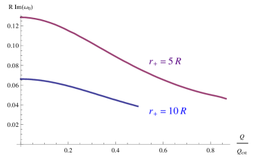
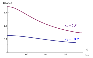
a)	b)

Figure 1: Imaginary part of the quasinormal frequency of the gravitational mode with $l=2$ for $r_{+}=5R$ and $r_{+}=10R$ as a function of the black hole charge: a) the “mostly-gravitational” or hydrodynamic sound mode; b) the “mostly-electromagnetic” or hydrodynamic diffusive mode. The frequency is given in units of the AdS curvature-radius $R$.

At finite electrostatic potential it is especially interesting to compare the results of our computation to the hydrodynamic approximation. As it was shown in Section 5, the position of the sound mode in the charged and neutral liquid is given by the same expression (35–36). Using the thermodynamic relation $\epsilon+p=Ts+\mu\rho$ and universal value for the shear viscosity $\eta=s/4\pi$ [15], we get:

$$\omega_{\rm hyd}=\pm\frac{1}{R}\sqrt{\frac{l(l+d-1)}{d}}-\frac{i(d-1)(l+d)l(l-1)}{4\pi dR^{2}}\frac{1}{T+\mu\frac{Q}{S}},$$

where $S$ and $Q$ are the total entropy and charge of the system. Substituting the values for temperature, charge, potential and entropy of the dual Reissner-Nordström black hole (18), we obtain the following final result for the sound mode frequency in the hydrodynamic regime

$$\omega_{\rm hyd}=\pm\frac{1}{R}\sqrt{\frac{l(l+d-1)}{d}}-\frac{i(d-1)(l+d)(l-1)}{d}\frac{r_{+}}{R^{2}+3r_{+}^{2}+3\mu^{2}R^{2}}.$$ (61)

Fig. 2 shows the relation between the numerical gravitational result and the hydrodynamic one for $l=2$ mode for different black hole temperatures. One can see that the curves approach unity quite fast and already at $T\approx 2R^{-1}$ the discrepancy is less than one percent, which is comparable to our numerical precision. This is a valuable check of the applicability of our procedure for calculating quasinormal modes.

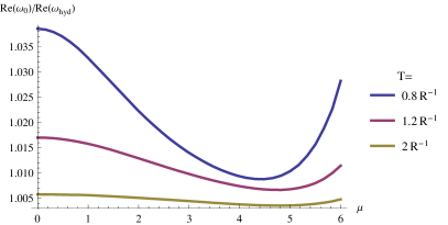
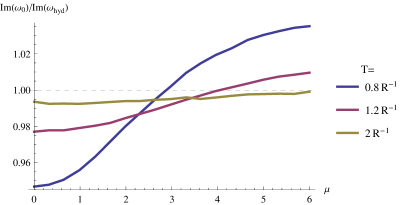
Figure 2: The relative values of the real and imaginary part of the quasinormal frequency at $l=2$ with respect to that given in the hydrodynamic approximation (61).

In case of the electromagnetic/diffusive channel we can perform a similar comparison with hydrodynamics. In [17] the diffusive constant for the CFT with zero chemical potential was obtained for any number of spatial directions

$$\mathcal{D}_{hyd}\big{|}_{\mu=0}=\frac{d+1}{d-1}\frac{1}{4\pi T}.$$ (62)

The comparison of our numerical results for the electromagnetic modes with this expectation is shown in Fig. 3. Again one can see, that the hydrodynamic approximation works quite well at relatively small temperature $T\sim 3R^{-1}$.

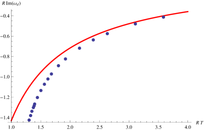
Figure 3: Comparison of the quasinormal frequencies in the diffusive/electromagnetic channel at zero chemical potential. Blue dots are the numerical results for QNMs of $Z_{1}^{+}$ for a black hole (57) while the red line is the hydrodynamics result for the CFT in $d=2$ (62).

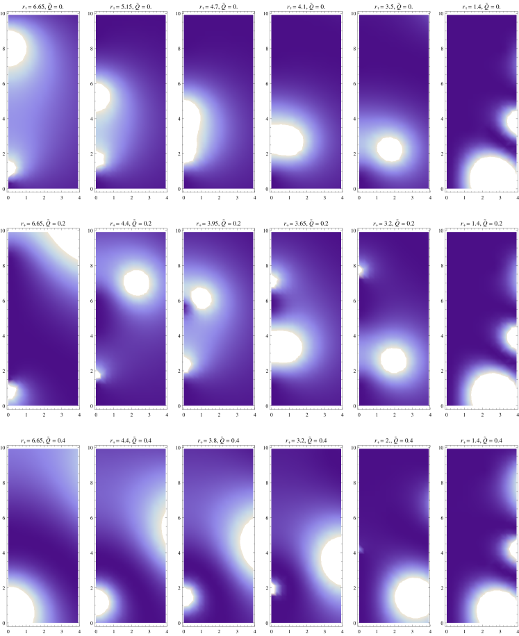
Figure 4: Position of the QNMs in the “mostly-electromagnetic” channel of the Reissner-Nordström black hole for various radii and charges in the complex $\omega$ plane. $\tilde{Q}=Q/Q_{ext}$, $r_{+}$ is measured in units of $R$ and frequency is measured in units of $R^{-1}$.

Using the numerical values of the quasinormal frequencies for various $T$ and $\mu$, we can calculate the value of the parameter $\mathfrak{q}$, which measures the classicality of the temperature fluctuations (14). It is interesting to study the transition to the quantum regime in both sound and diffusive contributions in (53). Looking at the behavior of the quasinormal frequencies in Fig. 1 one might conclude, that the diffusive mode violates the bound $\mathfrak{q}>1$ at large temperatures, as its quasinormal frequency is numerically large and, moreover, is inversely proportional to the temperature (62). However, observing the behavior of the actual gravitational quasinormal modes we see an interesting feature depicted on Fig. 4. Starting from large radii of the black hole, we see that in case of the neutral black hole the imaginary part of the hydrodynamic eigenmode first grows when the temperature is decreased, as expected from (62), but reaching the values $\approx i2R^{-1}$ it collides with another purely imaginary mode and recombines developing a pair of oscillating modes, which then travel back to the real axis maintaining the absolute value $|\omega_{d}|\approx 2R^{-1}$. This second purely imaginary mode behaves as $\omega\sim r_{+}$ and is a member of a series of the QNMs that one can typically find in the spectrum of spherical black holes [20, 22, 23].

Turning on a charge of the black hole does not change the picture substantially; again the hydrodynamic mode first moves away from the origin, but then it gets interfered with and substituted by the lowest mode from the series of spherical QNMs. Importantly, the mode which is closest to the origin never has an absolute value which is significantly bigger than $2R^{-1}$. Interestingly, the recombination of poles happens exactly in the region, where $\mathfrak{q}\approx 1$ for the diffusive mode.

A similar picture is found in the spectrum of the sound mode. The real part of the mode is defined by the speed of sound and does not change significantly with temperature, the imaginary part is numerically suppressed by a factor of 10, so its growth is negligible. At small radii the series of spherical modes with $|\omega|\sim r_{+}$ moves close to the hydrodynamic one. Again the closest mode is never farther from origin than $2R^{-1}$. These considerations allow us to draw the following conclusion. The transition to the quantum regime at low temperatures in the quantity $\mathfrak{q}=\frac{2\pi T}{|\omega_{0}|}$ happens for both modes approximately simultaneously, as the absolute values of the lowest modes $|\omega_{0}|$ are frozen near $2R^{-1}$ while the temperature keeps decreasing.

To illustrate this transition we plot the curve where $\mathfrak{q}=1$ – for simplicity for the sound mode – in the phase diagram of the charged black hole in AdS space in the grand canonical ensemble, i.e. for fixed temperature $T$ and asymptotic electrostatic potential $\mu$; see Fig. 5. It is not surprising, that at a decent value of the potential the curve behaves almost like a constant temperature line.

The phase diagram in Fig. 5 contains also the phase transition between the Reissner-Nordström black hole and the thermal gas of particles in the background of the extremal black hole with given potential $\mu$, denoted by AdS^∗ [30]. At zero charge this phase transition reduces to the Hawking-Page transition for the AdS-Schwarzschild black hole [4]. We find that the lowest value of the parameter $\mathfrak{q}$, which is achieved before this phase transition occurs, is $\mathfrak{q}\approx 0.92$ so the deep quantum regime is never reached for the neutral black hole. This is also supported by the peculiar behavior of the diffusive mode, discussed above. Instead one should speak about the region where quantum effects are becoming important.

The other interesting line in the phase diagram is the one describing the region, where the temperature fluctuations computed numerically via (6) using (9) for the gravitational quasinormal modes are of the order of the temperature itself. Linear response theory is no longer reliable below this line and it becomes meaningless to speak of small fluctuations, so we can plot it only approximately. Extremal black holes are thus not included in our treatment.

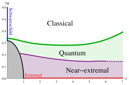
Figure 5: Phase structure of the charged black hole in AdS₄ in the grand canonical ensemble. The black line marks the “Hawking-Page type” phase transition [30]. The green line is $\mathfrak{q}=1$, and thus in the green region quantum effects become important. The purple line marks the region, where the numerically computed fluctuation $\left\langle\delta T^{2}\right\rangle^{1/2}$ is comparable to the temperature itself (at $\mu>6$ our precision does not allow us to continue the line reliably).

7 Discussion

We have studied temperature fluctuations in the holographic dual of the AdS-Reissner-Nordström black hole. Interestingly, temperature fluctuations are described by quasinormal modes of a black hole in both the sound channel, for which the oscillation frequencies are much larger than the attenuation rate, and diffusion channel, for which the quasinormal modes are purely damped. This leads to a rather specific behavior of temperature fluctuations. The transition from thermal to quantum fluctuations is found in the region where hydrodynamics is barely applicable and is governed by the peculiar behavior of electromagnetic and gravitational scalar quasinormal modes.

As expected, temperature fluctuations behave classically for a large black hole at high temperature and become more and more quantum as the black hole temperature is lowered. For the large black holes the fluctuations are mostly given by the contribution from the sound mode, whereas for small black holes in quantum region the contributions from sound and diffusive modes are of the same order. Temperature fluctuations of a neutral AdS black hole never become really quantum, because the black hole becomes thermodynamically unstable and undergoes the Hawking-Page phase transition when the fluctuations are about to enter the quantum regime. Temperature fluctuations of charged AdS black holes can, however, enter the quantum regime. At low temperatures the behavior of the fluctuations is mostly governed by the lowest poles from the series of QNMs of spherical black holes. It would be interesting to study this region in more detail in future work. At very low temperatures, for near-extremal black holes, fluctuations become so strong that one presumably cannot trust linear response theory any more. The strongly non-equilibrium behavior that then sets in can perhaps be analyzed along the lines of [31, 32, 33].

Acknowledgments

We thank Joe Bhaseen, Elias Kiritsis, David Tong and Daniel Brattan for useful comments and discussions. A. K. and S. B. G. thank the organizers of the HoloGrav network workshop “Holographic Methods and Applications” for hospitality.

The work of A. B. an Y. K. is supported by US DOE BES, ERC advanced grant DM 321-013 and by Swedish Research Council (VR) grant 2012-2983. The work of A. K. is partially supported by RFBR grant 12-02-00284-a and the Dynasty Foundation. The research of L.T. is supported in part by Icelandic Research Fund grant 130131-052 and by a grant from the University of Iceland Research Fund. The work of K.Z. is supported in part by the Marie Curie network GATIS of the European Union’s FP7 Programme under REA Grant Agreement No 317089, in part by ERC advanced grant No 341222 and by Swedish Research Council (VR) grant 2013-4329.

Appendix A Temperature fluctuations

A.1 The overdamped mode

Let us consider the integral

$$\langle\delta T^{2}\rangle=\frac{\hbar T}{2\pi C_{v}}\int_{-\infty}^{\infty}d\omega\;\frac{\omega\tau}{(\omega\tau)^{2}+1}\coth\left(\frac{\hbar\omega}{2T}\right)=\frac{\hbar T}{2\pi C_{v}\tau}\int_{-\infty}^{\infty}dx\;\frac{x}{x^{2}+1}\coth\left(\frac{x}{2\mathfrak{r}}\right),$$ (63)

where $x=\omega\tau$ and we have defined

$$\mathfrak{r}\equiv\frac{T\tau}{\hbar}.$$ (64)

We can now conveniently define

$$I\equiv\frac{2\pi C_{v}\tau}{\hbar T}\langle\delta T^{2}\rangle=\int_{-\infty}^{\infty}dx\;f,\qquad f\equiv\frac{x}{x^{2}+1}\coth\left(\frac{x}{2\mathfrak{r}}\right).$$ (65)

As $I$ is UV-divergent, we introduce a cutoff $x_{c}\equiv\omega_{c}\tau$: $I_{\rm reg}=\int_{-x_{c}}^{x_{c}}dx\;f$. Considering now the contour integral

$$I_{\gamma}=\oint_{\gamma}dz\;\frac{z}{z^{2}+1}\coth\left(\frac{z}{2\mathfrak{r}}\right),$$ (66)

where $\gamma$ is given in Fig. 6.

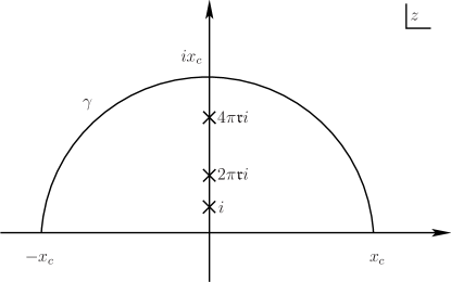
Figure 6: Contour $\gamma$ in the complex $x$ plane.

The contribution from the arc will vanish for $x_{c}\to\infty$, i.e.

$$\lim_{x_{c}\to\infty}I_{\gamma}=\lim_{x_{c}\to\infty}{\rm p.v.}~{}I_{\rm reg},$$ (67)

as long as the contour does not hit a pole on the imaginary axis.

Using residue theory, we have

$$I_{\gamma}=2\pi i\left[{\rm Res}(f,i)+\sum_{n=1}^{\Lambda}{\rm Res}(f,2n\pi\mathfrak{r}i)\right],\qquad\Lambda\equiv{\rm floor}\left(\frac{x_{c}}{2\pi\mathfrak{r}}\right).$$ (68)

The residues can be calculated easily

$${\rm Res}(f,i) =-\frac{i}{2}\cot\left(\frac{1}{2\mathfrak{r}}\right),$$ (69)

$${\rm Res}(f,2n\pi\mathfrak{r}i) =\frac{4n\pi\mathfrak{r}^{2}i}{1-4n^{2}\pi^{2}\mathfrak{r}^{2}},$$ (70)

and thus the contour integral reads

$$I_{\gamma}=\pi\cot\left(\frac{1}{2\mathfrak{r}}\right)-\sum_{n=1}^{\Lambda}\frac{8n\pi^{2}\mathfrak{r}^{2}}{1-4n^{2}\pi^{2}\mathfrak{r}^{2}}.$$ (71)

So far we did not assume anything about $\mathfrak{r}$ other than it being a real positive constant. In the limit $\mathfrak{r}\gg 2\pi$, we can expand the above expression to get

$$I_{\gamma}\simeq 2\pi\mathfrak{r}+2\sum_{n=1}^{\Lambda}\frac{1}{n},$$ (72)

where the last term is the harmonic sum, which is known to be divergent. Expressing the harmonic sum in terms of the cutoff, we have

$$I_{\gamma}\simeq 2\pi\mathfrak{r}-\frac{\pi}{6\mathfrak{r}}+2\log\left(\frac{x_{c}}{2\pi\mathfrak{r}}\right)+2\gamma_{E}+\mathcal{O}\left(\frac{\mathfrak{r}}{x_{c}},\frac{1}{\mathfrak{r}^{3}}\right),$$ (73)

where $\gamma_{E}$ is the Euler constant. Finally, we can write [7]

$$\langle\delta T^{2}\rangle=\frac{T^{2}}{C_{v}}\left[1-\frac{\hbar^{2}}{12T^{2}\tau^{2}}+\frac{\hbar}{\pi T\tau}\left(\log\left(\frac{\hbar\omega_{c}}{2\pi T}\right)+\gamma_{E}\right)+\mathcal{O}\left(\frac{1}{\omega_{c}\tau},\frac{\hbar^{4}}{(T\tau)^{4}}\right)\right],$$ (74)

where $\omega_{c}$ is the cut-off frequency.

In the opposite limit, $\mathfrak{r}\ll 2\pi$, the temperature fluctuations are in the quantum regime and can be approximated as follows. We neglect the residues coming from the response function and approximate the sum in (71) with an integral and obtain

$$I_{\gamma}\simeq\log x_{c}^{2},$$ (75)

which we can write as [7]

$$\langle\delta T^{2}\rangle\simeq\frac{\hbar T}{\pi C_{v}\tau}\log\omega_{c}\tau.$$ (76)

A more careful treatment of the arc is necessary because a simple power counting naively tells us that it is logarithmically divergent. We want to show that

$$\lim_{x_{c}\to\infty}\int_{C_{x_{c}}^{+}}dz\;\frac{z}{z^{2}+1}\coth\left(\frac{z}{2\mathfrak{r}}\right)=0,$$ (77)

where $C_{x_{c}}^{+}$ denotes the northern semicircle of radius $x_{c}$. The arc can be parametrized by $z=x_{c}e^{i\theta}$, where $\theta\in[0,\pi]$. Rewriting the coth, we have

$$\coth\left(\frac{z}{2\mathfrak{r}}\right)=\left(1+\frac{2e^{-z/\mathfrak{r}}}{1-e^{-z/\mathfrak{r}}}\right)=\left(-1-\frac{2e^{z/\mathfrak{r}}}{1-e^{z/\mathfrak{r}}}\right),$$ (78)

which we will use for the first and second quadrants of the $z$ plane, respectively. We therefore have

$$\int_{C_{x_{c}}^{+}}dz\;\frac{z}{z^{2}+1}\coth\left(\frac{z}{2\mathfrak{r}}\right) =\int_{C_{x_{c}}^{+1}}dz\;\frac{z}{z^{2}+1}\left(1+\frac{2e^{-z/\mathfrak{r}}}{1-e^{-z/\mathfrak{r}}}\right)+\int_{C_{x_{c}}^{+2}}dz\;\frac{z}{z^{2}+1}\left(-1-\frac{2e^{z/\mathfrak{r}}}{1-e^{z/\mathfrak{r}}}\right)$$

$$=I_{+1}^{\rm pol}+I_{+1}^{\exp}+I_{+2}^{\rm pol}+I_{+2}^{\exp}.$$ (79)

The integrals of the two polynomials in $z$ can be carried out

$$I_{+1}^{\rm pol}+I_{+2}^{\rm pol} =i\int_{0}^{\frac{\pi}{2}}d\theta\;\frac{x_{c}^{2}e^{i2\theta}}{x_{c}^{2}e^{i2\theta}+1}-i\int_{\frac{\pi}{2}}^{\pi}d\theta\;\frac{x_{c}^{2}e^{i2\theta}}{x_{c}^{2}e^{i2\theta}+1}=2\Re\left[i\int_{0}^{\frac{\pi}{2}}d\theta\;\frac{x_{c}^{2}e^{i2\theta}}{x_{c}^{2}e^{i2\theta}+1}\right]=-2\mathop{\rm arccoth}(x_{c}^{2}),$$ (80)

which goes to zero in the limit of $x_{c}\to\infty$. Now let us consider the first integral with exponentials

$$I_{+1}^{\exp}=\int_{C_{x_{c}}^{+1}}dz\;\frac{ze^{-z/\mathfrak{r}}}{(z^{2}+1)(1-e^{-z/\mathfrak{r}})}.$$ (81)

Since we are interested in the large $x_{c}$ behavior of this integral, let us instead consider

$$\tilde{I}_{+1}^{\exp}=\int_{C_{x_{c}}^{+1}}\frac{dz}{z}\;\frac{e^{-z/\mathfrak{r}}}{1-e^{-z/\mathfrak{r}}}=i\int_{0}^{\frac{\pi}{2}}d\theta\;\frac{\exp\left(-\frac{x_{c}}{\mathfrak{r}}e^{i\theta}\right)}{1-\exp\left(-\frac{x_{c}}{\mathfrak{r}}e^{i\theta}\right)}.$$ (82)

We will now need the lemma that

$$\left|\int_{a}^{b}dz\;f(z)\right|\leq\int_{a}^{b}dz\;M(z),$$ (83)

where $f(z)$ is a complex function and $M(z)$ is a real-valued function on the real interval $[a,b]$ such that $|f(z)|\leq M(z)$ everywhere on said interval (to prove this lemma, compose the integral into Riemann sums and use the triangle inequality). Hence we can write

$$|\tilde{I}_{+1}^{\exp}|\leq\int_{0}^{\frac{\pi}{2}}d\theta\;\frac{e^{-\frac{x_{c}}{\mathfrak{r}}\cos\theta}}{\sqrt{1+e^{-\frac{2x_{c}}{\mathfrak{r}}\cos\theta}-2e^{-\frac{x_{c}}{\mathfrak{r}}\cos\theta}\cos\left(\frac{x_{c}}{\mathfrak{r}}\sin\theta\right)}}.$$ (84)

To simplify the problem we will now assume that $x_{c}=(2m+1)\pi\mathfrak{r}$ with $m$ being an integer. This value of the cut off is chosen such that the contour goes right in the middle between the Matsubara poles on the imaginary axis. We can now write

$$|\tilde{I}_{+1}^{\exp}|\leq A\int_{0}^{\frac{\pi}{2}}d\theta\;\exp\left(-\frac{x_{c}}{\mathfrak{r}}\cos\theta\right)=\frac{A\pi}{2}\left[I_{0}\big{(}(2m+1)\pi\big{)}-L_{0}\big{(}(2m+1)\pi\big{)}\right],$$ (85)

where $A\gtrsim 1$ is a constant of order one taking on the minimum value of the denominator of eq. (84). Expanding the above expression for large $m$, we have

$$|\tilde{I}_{+1}^{\exp}|\leq\frac{A}{(2m+1)\pi}+\mathcal{O}(m^{-3}),$$ (86)

which clearly goes to zero for $m\to\infty$. The same proof can be applied to $I_{+2}^{\exp}$ and hence is bounded by the same numerical value.

A.2 The underdamped mode

Let us now consider the integral

$$\langle\delta T^{2}\rangle=\frac{\hbar T}{2\pi C_{v}}\int_{-\infty}^{\infty}d\omega\;\frac{2\omega\Gamma\Omega^{2}}{(\omega^{2}-\Omega^{2})^{2}+4\omega^{2}\Gamma^{2}}\coth\left(\frac{\hbar\omega}{2T}\right)=\frac{\hbar T\Omega^{2}}{\pi C_{v}\Gamma}\int_{-\infty}^{\infty}dx\;\frac{x}{(x^{2}-\mathfrak{a}^{2})^{2}+4x^{2}}\coth\left(\frac{x}{2\mathfrak{b}}\right),$$ (87)

where we have defined

$$x\equiv\frac{\omega}{\Gamma},\qquad\mathfrak{a}\equiv\frac{\Omega}{\Gamma},\qquad\mathfrak{b}\equiv\frac{T}{\hbar\Gamma}.$$ (88)

We will assume that $\mathfrak{a}>1$. We can now conveniently define

$$I\equiv\frac{\pi C_{v}\Gamma}{\hbar T\Omega^{2}}\langle\delta T^{2}\rangle=\int_{-\infty}^{\infty}dx\;f,\qquad f\equiv\frac{x}{(x^{2}-\mathfrak{a}^{2})^{2}+4x^{2}}\coth\left(\frac{x}{2\mathfrak{b}}\right).$$ (89)

Notice that for this response function, the integral is no longer divergent. Consider now the contour integral

$$I_{\gamma}=\oint_{\gamma}dz\;\frac{z}{(z^{2}-\mathfrak{a}^{2})^{2}+4z^{2}}\coth\left(\frac{z}{2\mathfrak{b}}\right),$$ (90)

where $\gamma$ is given in Fig. 7.

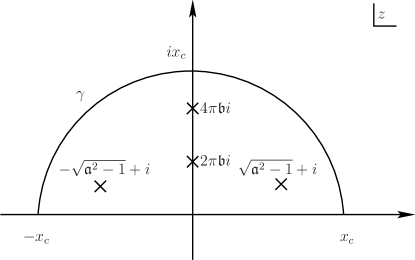
Figure 7: Contour $\gamma$ in the complex plane.

The contribution from the arc will vanish for $x_{c}\to\infty$ and $x_{c}\neq 2\pi\mathfrak{b}n$, meaning that the cutoff does not make the contour cut through a pole, and thus

$$\lim_{x_{c}\to\infty}I_{\gamma}=\lim_{x_{c}\to\infty}{\rm p.v.}~{}I.$$ (91)

It is easy to estimate that the contribution from the arc will be of the order of $1/x_{c}^{2}$.

We have two types of contributions, the first is due to the two classical poles at $\pm\sqrt{\mathfrak{a}^{2}-1}+i$ and the second comes from the $n$-th Matsubara mode at $2n\pi\mathfrak{b}i$,

$$I_{\gamma}=2\pi i\left[\sum_{\pm}{\rm Res}(f,\pm\sqrt{\mathfrak{a}^{2}-1}+i)+\sum_{n=1}^{\Lambda}{\rm Res}(f,2n\pi\mathfrak{b}i)\right],\qquad\Lambda\equiv{\rm floor}\left(\frac{x_{c}}{2\pi\mathfrak{b}}\right).$$ (92)

The residues can be calculated easily

$$\sum_{\pm}{\rm Res}(f,\pm\sqrt{\mathfrak{a}^{2}-1}+i) =-\frac{i}{8\sqrt{\mathfrak{a}^{2}-1}}\sum_{\pm}\coth\left(\frac{\pm i+\sqrt{\mathfrak{a}^{2}-1}}{2\mathfrak{b}}\right),$$ (93)

$${\rm Res}(f,2n\pi\mathfrak{b}i) =\frac{4n\pi\mathfrak{b}^{2}i}{\left(4n^{2}\pi^{2}\mathfrak{b}^{2}+\mathfrak{a}^{2}\right)^{2}-16n^{2}\pi^{2}\mathfrak{b}^{2}},$$ (94)

and thus the contour integral reads

$$I_{\gamma}=\frac{\pi}{2\sqrt{\mathfrak{a}^{2}-1}}\frac{\sinh\frac{\sqrt{\mathfrak{a}^{2}-1}}{\mathfrak{b}}}{\cosh\frac{\sqrt{\mathfrak{a}^{2}-1}}{\mathfrak{b}}-\cos\frac{1}{\mathfrak{b}}}-\sum_{n=1}^{\Lambda}\frac{8n\pi^{2}\mathfrak{b}^{2}}{\left(4n^{2}\pi^{2}\mathfrak{b}^{2}+\mathfrak{a}^{2}\right)^{2}-16n^{2}\pi^{2}\mathfrak{b}^{2}}.$$ (95)

We will now consider the classical regime, which can be seen from Fig. 7 to be where

$$2\pi\mathfrak{b}\gg\mathfrak{a},\qquad{\rm or\ equivalently}\qquad T\gg\frac{\hbar\Omega}{2\pi},$$ (96)

which corresponds to the situation in which the classical poles are reached at much lower frequencies (in the complex plane) than the Matsubara modes. The classicality parameter (14) is given is by $\mathfrak{q}=2\pi\mathfrak{b}/\mathfrak{a}$, so we can see the how the classicality is manifested in the approximation. It will be instructive to expand the above contour integral for $2\pi\mathfrak{b}\gg\mathfrak{a}>1$,

$$I_{\gamma}\simeq\frac{\pi\mathfrak{b}}{\mathfrak{a}^{2}}+\frac{\pi}{12\mathfrak{b}}-\frac{\zeta(3)}{2\pi^{2}\mathfrak{b}^{2}}+\mathcal{O}\left(\frac{1}{\mathfrak{b}^{3}}\right),$$ (97)

which we can write as

$$\langle\delta T^{2}\rangle\simeq\frac{T^{2}}{C_{v}}\left[1+\frac{\hbar^{2}\Omega^{2}}{12T^{2}}-\frac{\hbar^{3}\zeta(3)\Omega^{2}\Gamma}{2\pi^{3}T^{3}}+\mathcal{O}\left(\frac{\hbar^{4}\Omega^{2}\Gamma^{2}}{T^{4}}\right)\right].$$ (98)

If $\mathfrak{b}\ll\sqrt{\mathfrak{a}^{2}-1}$, then the contour integral (95) can be approximated to be

$$I_{\gamma}\simeq\frac{\pi}{2\sqrt{\mathfrak{a}^{2}-1}}\left[\frac{1}{2}+\frac{1}{\pi}\arctan\left(\frac{\mathfrak{a}^{2}-2}{2\sqrt{\mathfrak{a}^{2}-1}}\right)+\mathcal{O}\left(\frac{\mathfrak{b}^{2}}{\mathfrak{a}^{4}}\right)\right].$$ (99)

If furthermore $\mathfrak{a}\gg 1$, the above expression simplifies as follows

$$I_{\gamma}\simeq\frac{\pi}{2\mathfrak{a}}-\frac{1}{\mathfrak{a}^{2}}+\mathcal{O}\left(\frac{1}{\mathfrak{a}^{3}},\frac{\mathfrak{b}^{2}}{\mathfrak{a}^{4}}\right),$$ (100)

which we can write as

$$\langle\delta T^{2}\rangle\simeq\frac{\hbar T\Omega}{2C_{v}}-\frac{\hbar T\Gamma}{\pi C_{v}}+T\Omega\mathcal{O}\left(\frac{\Gamma^{2}}{\Omega^{2}},\frac{T^{2}\Gamma}{\Omega^{3}}\right).$$ (101)

When $\mathfrak{a}<1$, the modes become those of the overdamped regime.

Appendix B Thermodynamics of the fluid with conserved charge

In this Appendix we derive the thermodynamic identities used throughout the text. Most of them may be looked up in [16] or derived straightforwardly with the help of any textbook on thermodynamics but we find it useful to write them here for reference.

In [16] one can find the following treatment. Consider the change of the energy divided by the volume surrounding one particle $dE/V$. In this case on has $V\sim n^{-1}$, $dV/V=-dn/n$ and one uses the thermodynamic equations valid in the grand canonical ensemble

$$\frac{dE}{V}=\frac{d(\epsilon V)}{V}=d\epsilon-\epsilon\frac{dn}{n}.$$ (102)

On the other hand $dE=TdS-PdV$, hence $\frac{T}{V}dS=d\epsilon-w\frac{dn}{n}$, where $w$ is the enthalpy density. Then the variation of the pressure is

$$dp=\frac{\partial p}{\partial\epsilon}\bigg{|}_{n}d\epsilon+\frac{\partial p}{\partial n}\bigg{|}_{\epsilon}dn=\left[\beta_{1}+\frac{n}{w}\beta_{2}\right]d\epsilon-\beta_{2}\frac{n}{w}\frac{TdS}{V},$$ (103)

using the notation for the thermodynamic derivatives introduced in eq. (41). Hence the speed of sound is

$$v_{s}^{2}=\left[\beta_{1}+\frac{n}{w}\beta_{2}\right]=\frac{\partial p}{\partial\epsilon}\bigg{|}_{S,N}\,.$$ (104)

Let us introduce some more useful thermodynamic identities, using a convenient formalism involving Jacobians

$$\frac{\partial(A,B)}{\partial(C,D)}\equiv\frac{\partial A}{\partial C}\bigg{|}_{D}\frac{\partial B}{\partial D}\bigg{|}_{C}-\frac{\partial A}{\partial D}\bigg{|}_{C}\frac{\partial B}{\partial C}\bigg{|}_{D}.$$ (105)

This allows us to rewrite

$$T\left.\frac{\partial\epsilon}{\partial T}\right|_{\mu/T}=T\frac{\frac{\partial(\epsilon,\mu/T)}{\partial(\mu,T)}}{\frac{\partial(T,\mu/T)}{\partial(\mu,T)}}=\mu\left.\frac{\partial\epsilon}{\partial\mu}\right|_{T}+T\left.\frac{\partial\epsilon}{\partial T}\right|_{\mu}.$$ (106)

Similarly,

$$T\left.\frac{\partial n}{\partial T}\right|_{\mu/T}=\mu\left.\frac{\partial n}{\partial\mu}\right|_{T}+T\left.\frac{\partial n}{\partial T}\right|_{\mu}.$$ (107)

Using the identity $d\epsilon=Tds+\mu dn$, this can be rewritten as

$$T\left.\frac{\partial n}{\partial T}\right|_{\mu/T}=\left.\frac{\partial\epsilon}{\partial\mu}\right|_{T}-T\left[\left.\frac{\partial s}{\partial\mu}\right|_{T}-\left.\frac{\partial n}{\partial T}\right|_{\mu}\right]=\left.\frac{\partial\epsilon}{\partial\mu}\right|_{T}.$$ (108)

The term in the square brackets is zero by a Maxwell relation, because it may be expressed via the second derivatives of the thermodynamic potential $dw=-sdT-nd\mu=-dp$ (because $w=-p$) in the grand canonical ensemble:

$$s=\frac{\partial p}{\partial T}\bigg{|}_{\mu},\qquad n=\frac{\partial p}{\partial\mu}\bigg{|}_{T}.$$ (109)

Using eqs. (106) and (108) we can reexpress the coefficients, $\alpha$, from (41) as

$$\alpha_{1} =T\frac{\partial(\mu/T)}{\partial\epsilon}\bigg{|}_{n}=T\frac{\frac{\partial(\mu/T,n)}{\partial(\mu/T,T)}}{\frac{\partial(\epsilon,n)}{\partial(\mu/T,T)}}=\frac{1}{TD}\frac{\partial\epsilon}{\partial\mu}\bigg{|}_{T},$$ (110)

$$\alpha_{2} =T\frac{\partial(\mu/T)}{\partial n}\bigg{|}_{\epsilon}=T\frac{\frac{\partial(\mu/T,\epsilon)}{\partial(\mu/T,T)}}{\frac{\partial(n,\epsilon)}{\partial(\mu/T,T)}}=-\frac{1}{D}\left[\frac{\partial\epsilon}{\partial T}\bigg{|}_{\mu}+\frac{\mu}{T}\frac{\partial\epsilon}{\partial\mu}\bigg{|}_{T}\right],$$ (111)

where we again have used the Maxwell relation and $D$ in the denominator is given by

$$D=\frac{\partial\epsilon}{\partial\mu}\bigg{|}_{T}\frac{\partial n}{\partial T}\bigg{|}_{\mu/T}-\frac{\partial n}{\partial\mu}\bigg{|}_{T}\frac{\partial\epsilon}{\partial T}\bigg{|}_{\mu/T} =\frac{1}{T}\frac{\partial\epsilon}{\partial\mu}\bigg{|}_{T}\frac{\partial\epsilon}{\partial\mu}\bigg{|}_{T}-\frac{\partial n}{\partial\mu}\bigg{|}_{T}\left(\frac{\mu}{T}\frac{\partial\epsilon}{\partial\mu}\bigg{|}_{T}+\frac{\partial\epsilon}{\partial T}\bigg{|}_{\mu}\right)=$$

$$=\frac{1}{T}\frac{\partial\epsilon}{\partial\mu}\bigg{|}_{T}T\frac{\partial s}{\partial\mu}\bigg{|}_{T}-\frac{\partial n}{\partial\mu}\bigg{|}_{T}\frac{\partial\epsilon}{\partial T}\bigg{|}_{\mu}=\frac{\partial(\epsilon,n)}{\partial(\mu,T)}.$$ (112)

To proceed with the coefficients, $\beta$, defined in eq. (42) we use (109)

$$\beta_{1} =\frac{\partial p}{\partial\epsilon}\bigg{|}_{n}=\frac{1}{D}\frac{\partial(p,n)}{\partial(\mu,T)}=\frac{1}{D}\left(n\frac{\partial s}{\partial\mu}\bigg{|}_{T}-s\frac{\partial n}{\partial\mu}\bigg{|}_{T}\right),$$ (113)

$$\beta_{2} =\frac{\partial p}{\partial n}\bigg{|}_{\epsilon}=-\frac{1}{D}\frac{\partial(p,\epsilon)}{\partial(\mu,T)}=-\frac{1}{D}\left(n\frac{\partial\epsilon}{\partial T}\bigg{|}_{\mu}-s\frac{\partial\epsilon}{\partial\mu}\bigg{|}_{T}\right).$$ (114)

Now one can show that

$$w\alpha_{1}+n\alpha_{2} =-\frac{1}{D}\left[-\frac{\epsilon+p}{T}\frac{\partial\epsilon}{\partial\mu}\bigg{|}_{T}+\frac{n\mu}{T}\frac{\partial\epsilon}{\partial\mu}\bigg{|}_{T}+n\frac{\partial\epsilon}{\partial T}\bigg{|}_{\mu}\right]=\beta_{2},$$ (115)

$$n\alpha_{1}-\beta_{1} =\frac{1}{D}\left(\frac{n\mu}{T}\frac{\partial n}{\partial\mu}\bigg{|}_{T}+s\frac{\partial n}{\partial\mu}\bigg{|}_{T}\right)=\frac{w}{DT}\frac{\partial n}{\partial\mu}\bigg{|}_{T}\equiv-w\alpha_{3},$$ (116)

and in turn it follows that $\alpha_{2}\beta_{1}-\alpha_{1}\beta_{2}=w(\alpha_{2}\alpha_{3}-\alpha_{1}^{2})$, $n\alpha_{2}-\beta_{2}=w\alpha_{1}$ from which we can write eq. (48). We have introduced the quantity $\alpha_{3}$ with which one can show that the following holds

$$\alpha_{1}^{2}-\alpha_{2}\alpha_{3} =\frac{1}{D^{2}T}\left[\frac{\partial\epsilon}{\partial\mu}\bigg{|}_{T}\left(\frac{1}{T}\frac{\partial\epsilon}{\partial\mu}\bigg{|}_{T}-\frac{\mu}{T}\frac{\partial n}{\partial\mu}\bigg{|}_{T}\right)-\frac{\partial\epsilon}{\partial T}\bigg{|}_{\mu}\frac{\partial n}{\partial\mu}\bigg{|}_{T}\right]=\frac{1}{D^{2}T}\frac{\partial(\epsilon,n)}{\partial(\mu,T)}=\frac{1}{DT},$$ (117)

where we used the same tricks as in (112). Using Jacobians, it can be seen that

$$\alpha_{3}=\frac{1}{DT}\left.\frac{\partial n}{\partial\mu}\right|_{T}=\frac{1}{T}\left.\frac{\partial T}{\partial\epsilon}\right|_{n},$$

as indicated in the main text.

When calculating the correlator of temperature fluctuations we encounter the following expressions

$$\frac{\partial T}{\partial\epsilon}\bigg{|}_{n} =\frac{\partial(T,n)}{\partial(\epsilon,n)}=-\frac{1}{D}\frac{\partial(T,n)}{\partial(T,\mu)}=-\frac{1}{D}\frac{\partial n}{\partial\mu}\bigg{|}_{T},$$ (118)

$$\frac{\partial T}{\partial n}\bigg{|}_{\epsilon} =\frac{\partial(T,\epsilon)}{\partial(n,\epsilon)}=\frac{1}{D}\frac{\partial(T,\epsilon)}{\partial(T,\mu)}=\frac{1}{D}\frac{\partial\epsilon}{\partial\mu}\bigg{|}_{T}.$$ (119)

Hence, we can rewrite the expression one finds in the numerator of the fluctuation amplitude in classical limit (48) as

$$\left(\frac{\partial T}{\partial\epsilon}\bigg{|}_{n}\right)^{2}\alpha_{2}-2\frac{\partial T}{\partial\epsilon}\bigg{|}_{n}\frac{\partial T}{\partial n}\bigg{|}_{\epsilon}\alpha_{1}+\left(\frac{\partial T}{\partial n}\bigg{|}_{\epsilon}\right)^{2}\alpha_{3}=$$

$$=-\frac{1}{D^{3}}\frac{\partial n}{\partial\mu}\bigg{|}_{T}\left(\frac{\partial n}{\partial\mu}\bigg{|}_{T}\frac{\partial\epsilon}{\partial T}\bigg{|}_{\mu}+\frac{\partial n}{\partial\mu}\bigg{|}_{T}\frac{\mu}{T}\frac{\partial\epsilon}{\partial\mu}\bigg{|}_{T}-\frac{1}{T}\frac{\partial\epsilon}{\partial\mu}\bigg{|}_{T}\right)=-\frac{1}{D^{2}}\frac{\partial n}{\partial\mu}\bigg{|}_{T}=\frac{1}{D}\frac{\partial T}{\partial\epsilon}\bigg{|}_{n}=\frac{1}{Dc_{v}}.$$ (120)

In the last equation the volumetric heat capacity is defined at constant self-volume of one particle, which means $V\sim 1/n={\rm const}$. Finally, (48) is obtained by combining (117) and (120).

Appendix C Calculation of the scalar quasinormal modes of an AdS-Reissner-Nordström black hole

C.1 Boundary conditions

The equations of motion, which describe the coupled fluctuations of the metric and electromagnetic field on the background of a Reissner-Nordström black hole in 4-dimensional de Sitter space were obtained in [24] following the procedure outlined in [29]. The equations of motion for the AdS case can be obtained simply by considering a negative cosmological constant $\Lambda=-\frac{3}{R^{2}}$. The notation used in this section differs from the one used in the rest of the paper, but we adopt it in order to facilitate reference to [24, 29] keeping in mind that the final result (quasinormal frequencies) will be easy to interpret.

The background metric is

$$ds^{2}=e^{2\nu}dt^{2}-e^{2\psi}d\phi^{2}-e^{2\mu_{2}}dr^{2}-e^{2\mu_{3}}d\theta^{2},$$ (121)

where

$$e^{2\nu}=\frac{\Delta}{r^{2}},\quad e^{2\mu_{2}}=\frac{r^{2}}{\Delta},\quad e^{2\mu_{3}}=r^{2},\quad e^{2\psi}=r^{2}\sin^{2}\theta,$$ (122)

and

$$\Delta=r^{2}-2Mr+Q^{2}+\frac{r^{4}}{R^{2}}.$$ (123)

The background electromagnetic field is described by a single component of the field-strength tensor

$$F_{tr}=-\frac{Q}{r^{2}}.$$ (124)

The polar (even with respect to the change of sign of $\phi$) mode involves the fluctuations of the metric $\delta\nu,\delta\mu_{2},\delta\mu_{3},\delta\psi$ and of the field-strength tensor $\delta F_{tr},F_{t\theta},F_{r\theta}$. The fluctuations with angular momentum $l$ and the frequency $\omega$ may be described in the following way

$$\delta\nu =N(r)P_{l}(\theta), \delta F_{tr} =\frac{r^{2}e^{2\nu}}{2Q}B_{tr}(r)P_{l},$$ (125)

$$\delta\mu_{2} =L(r)P_{l}(\theta), F_{t\theta} =-\frac{re^{\nu}}{2Q}B_{t\theta}P_{l,\theta},$$ (126)

$$\delta\mu_{3} =T(r)P_{l}+V(r)P_{l,\theta,\theta}, F_{r\theta} =-\frac{i\omega re^{-\nu}}{2Q}B_{r\theta}(r)P_{l,\theta},$$ (127)

$$\delta\psi =T(r)P_{l}+V(r)P_{l,\theta}\cot\theta.$$

Introducing the parameters

$$\mu^{2} =2n=(l-1)(l+2),$$ (128)

$$p_{1} =3M+(9M^{2}+4Q^{2}\mu^{2})^{1/2},$$ (129)

$$p_{2} =3M-(9M^{2}+4Q^{2}\mu^{2})^{1/2},$$

one can rewrite the Einstein equations for fluctuations

$$\delta R_{ab}=-2\left[\eta^{nm}(\delta F_{an}F_{bm}+F_{an}\delta F_{bm})-\eta_{ab}Q\delta F_{tr}/r^{2}\right]$$ (130)

as a system of differential equations of first order [24]

$$N_{,r}=aN+bL+c(nV-B_{r\theta}),$$ (131)

$$L_{,r}=\left(a-\frac{1}{r}+\nu_{,r}\right)N+\left(b-\frac{1}{r}-\nu_{,r}\right)L+c(nV-B_{r\theta})-\frac{2}{r}B_{r\theta},$$ (132)

$$nV_{,r}=-\left(a-\frac{1}{r}+\nu_{,r}\right)N-\left(b+\frac{1}{r}-2\nu_{,r}\right)L-\left(c+\frac{1}{r}-\nu_{,r}\right)(nV-B_{r\theta})+B_{t\theta},$$ (133)

$$B_{t\theta}={B_{r\theta}}_{,r}+\frac{2}{r}B_{r\theta},$$ (134)

$$r^{4}e^{2\nu}B_{tr}=2Q^{2}\left[2T-l(l+1)V\right]-l(l+1)r^{2}B_{r\theta},$$ (135)

$$(r^{2}e^{2\nu}B_{t\theta})_{,r}+r^{2}e^{2\nu}B_{tr}+\omega^{2}r^{2}e^{-2\nu}B_{r\theta}=2Q^{2}\frac{N+L}{r},$$ (136)

where

$$a =\frac{n+1}{r}e^{-2\nu},$$ (137)

$$b =-\frac{1}{r}+\nu_{,r}+r\nu^{2}_{,r}+\omega^{2}e^{-4\nu}r-2\frac{e^{-2\nu}}{r^{3}}Q^{2}-\frac{ne^{-2\nu}}{r},$$ (138)

$$c =-\frac{1}{r}+r\nu^{2}_{,r}+\omega^{2}e^{-4\nu}r-\frac{2e^{-2\nu}}{r^{3}}Q^{2}+\frac{e^{-2\nu}}{r}.$$ (139)

These equations can be decoupled upon introducing the functions

$$Z_{1}^{+} =p_{1}H_{1}^{+}+(-p_{1}p_{2})^{1/2}H_{2}^{+},$$ (140)

$$Z_{2}^{+} =-(-p_{1}p_{2})^{1/2}H_{1}^{+}+p_{1}H_{2}^{+},$$ (141)

where

$$H_{1}^{+} =-\frac{1}{Q\mu}\left[r^{2}B_{r\theta}+2Q^{2}\frac{r}{\bar{\omega}}(L+nV-B_{r\theta})\right],$$ (142)

$$H_{2}^{+} =rV-\frac{r^{2}}{\bar{\omega}}(L+nV-B_{r\theta}),$$ (143)

and

$$\bar{\omega}=nr+3M-\frac{2Q^{2}}{r}.$$ (144)

The system can be reduced to the couple of equations

$$\frac{\Delta}{r^{2}}\frac{d}{dr}\left(\frac{\Delta}{r^{2}}\frac{d}{dr}Z_{i}^{+}\right)+\omega^{2}Z_{i}^{+}=V_{i}^{+}Z_{i}^{+}\qquad(i=1,2)$$ (145)

with Schrödinger-type potentials

$$V_{1}^{+} =\frac{\Delta}{r^{5}}\left[U+\frac{1}{2}(p_{1}-p_{2})W\right],$$ (146)

$$V_{2}^{+} =\frac{\Delta}{r^{5}}\left[U-\frac{1}{2}(p_{1}-p_{2})W\right],$$ (147)

where

$$U =\left(2nr+3M\right)W+\left(\bar{\omega}-nr-M+2\frac{r^{3}}{R^{2}}\right)-\frac{2nr^{2}}{\bar{\omega}}e^{2\nu},$$ (148)

$$W =\frac{\Delta}{r\bar{\omega}^{2}}(2nr+3M)+\frac{1}{\bar{\omega}}\left(nr+M-2\frac{r^{3}}{R^{2}}\right).$$ (149)

At this point it is useful to note, that for vanishing charge ($Q\rightarrow 0$) the potential $V_{2}^{+}$ reduces to the potential for purely gravitational polar fluctuations of the Schwarzschild black hole in AdS [22]. It is not surprising, because in this limit $p_{2}$ vanishes and hence $Z_{2}^{+}$ reduces to purely gravitational fluctuations $H_{2}^{+}$ plus a term proportional to $B_{r\theta}$, which vanishes itself according to the definition $B_{r\theta}\sim QF_{r\theta}$ (127). Similarly, in this limit the mode described by $Z_{1}^{+}$ corresponds to purely electromagnetic fluctuations on the background of the neutral black hole. Keeping these connections in mind at nonzero $Q$, we will still call the modes associated with $Z_{1}^{+}$ and $Z_{2}^{+}$ “electromagnetic” and “gravitational”, respectively.

In what follows, we will consider the fluctuations described by $Z_{i}^{+}$ and recover the asymptotic behavior of the metric fields in this mode. In order to do this, we need to complete the solution of (131-136) following the procedure outlined in [29]. First of all, we note that the sum of (132) and (133) after the substitution of (134) may be written as

$$L_{,r}+\left(\frac{2}{r}-\nu_{,r}\right)L=-\left[X_{,r}+\left(\frac{1}{r}-\nu_{,r}\right)X\right],$$ (150)

where

$$X=nV-B_{r\theta}.$$ (151)

On the other hand, we notice that the linear combination of $H_{1}^{+}$ and $H_{2}^{+}$, which we denote by $Z^{*}$, is expressed in terms of $L$ and $X$ as

$$Z^{*}=nH_{2}^{+}+\frac{Q\mu}{r}H_{1}^{+} =\frac{1}{\bar{\omega}}(3Mr-4Q^{2})X-\frac{1}{\bar{\omega}}(nr^{2}+2Q^{2})L$$ (152)

$$=rX-\frac{nr^{2}+2Q^{2}}{\bar{\omega}}(L+X).$$

Substituting $X$ from this expression into (150) we get

$$\bar{\omega}\frac{d}{dr}\left(\frac{r^{3}e^{-\nu}}{3Mr-4Q^{2}}L\right)=-r\frac{d}{dr}\left(re^{-\nu}\frac{\bar{\omega}}{3Mr-4Q^{2}}Z^{*}\right).$$ (153)

The expression for $L$ is thus obtained via the integral

$$L =-\frac{3Mr-4Q^{2}}{r^{3}e^{-\nu}}\int dr\frac{r}{\bar{\omega}}\frac{d}{dr}\left(re^{-\nu}\frac{\bar{\omega}}{3Mr-4Q^{2}}Z^{*}\right)$$ (154)

$$=-\frac{1}{r}Z^{*}+\frac{3Mr-4Q^{2}}{r^{3}e^{-\nu}}\left[\int dr\frac{e^{-\nu}}{\bar{\omega}}Z^{*}+C\right],$$

where in the second line we have performed an integration by parts and $C$ is an integration constant. However, the expression for $X$ can similarly be obtained by substituting $L$ of (152) into (150). After the integration by parts it reads

$$X=\frac{1}{r}Z^{*}+\frac{nr^{2}+2Q^{2}}{r^{3}e^{-\nu}}\left[\int dr\frac{e^{-\nu}}{\bar{\omega}}Z^{*}+C\right].$$ (155)

One can check, that the constants of integration in (154) and (155) are consistent by plugging these expressions into (150). We notice that the sum of $L$ and $X$ assumes a concise form

$$L+X=\frac{\bar{\omega}}{r^{2}e^{-\nu}}\left[\int dr\frac{e^{-\nu}}{\bar{\omega}}Z^{*}+C\right].$$ (156)

To proceed with the evaluation of $N$, we take the derivative (152) and substitute the expression of $(L+X)_{,r}$ from (150)

$$Z^{*}_{,r}=rX_{,r}+\left(\frac{3Mr-4Q^{2}}{r\bar{\omega}}\right)X-r^{2}e^{-\nu}\frac{d}{dr}\left(\frac{1}{r^{2}e^{-\nu}}\frac{nr^{2}+2Q^{2}}{\bar{\omega}}\right)(L+X).$$ (157)

Finally, we use equations (133) and (134) to eliminate $X_{,r}$ and obtain the expression for $N$

$$N =\frac{1}{ra-1+r\nu_{,r}}\bigg{\{}\frac{2}{r}B_{r\theta}-\frac{d}{dr}Z^{*}-$$ (158)

$$-\left[rb+1-2r\nu_{,r}+r^{2}e^{-\nu}\frac{d}{dr}\left(\frac{1}{r^{2}e^{-\nu}}\frac{nr^{2}+2Q^{2}}{\bar{\omega}}\right)\right]\frac{\bar{\omega}}{r^{2}e^{-\nu}}\left(\int dr\frac{e^{-\nu}}{\bar{\omega}}Z^{*}+C\right)+$$

$$+\left(\frac{3Mr-4Q^{2}}{r\bar{\omega}}-ar\right)\left[\frac{1}{r}Z^{*}+\frac{nr^{2}+2Q^{2}}{r^{3}e^{-\nu}}\left(\int dr\frac{e^{-\nu}}{\bar{\omega}}Z^{*}+C\right)\right]\bigg{\}}.$$

Let us now turn to the asymptotic behavior of the master functions $Z_{1}^{+}$ and $Z_{2}^{+}$. The corresponding Schrödinger equations at large $r$ take the form

$$\left(\frac{r^{2}}{R^{4}}\partial_{r}r^{2}\partial_{r}+\omega^{2}-\frac{\mu^{2}+2}{R^{2}}-\frac{2p_{1}^{2}}{\mu^{4}R^{4}}\right)Z_{2}^{+} =0,$$ (159)

$$\left(\frac{r^{2}}{R^{4}}\partial_{r}r^{2}\partial_{r}+\omega^{2}-\frac{\mu^{2}+2}{R^{2}}-\frac{2p_{2}^{2}}{\mu^{4}R^{4}}\right)Z_{1}^{+} =0.$$ (160)

As expected in the limit $Q\rightarrow 0$ the equation for $Z_{2}^{+}$ reduces to that of the Schwarzschild black hole in [14]. Hence, for large $r$, the asymptotics of the master functions can be expressed as sums of linearly independent modes

$$Z_{2}^{+}\Big{|}_{r\rightarrow\infty} =\alpha+\frac{\beta}{r},$$

$$Z_{1}^{+}\Big{|}_{r\rightarrow\infty} =\gamma+\frac{\delta}{r}.$$

From (140), (141) we get the expressions for $H_{1}^{+}$ and $H_{2}^{+}$ and from (152) the asymptotic expression for $Z^{*}$

$$Z^{*}=\xi+\frac{\eta}{r}+\frac{\zeta}{r^{2}},$$ (161)

where

$$\xi =\frac{n\big{(}p_{1}\alpha+\sqrt{-p_{1}p_{2}}\ \gamma\big{)}}{p_{1}(p_{1}-p_{2})},$$ (162)

$$\eta =\frac{n\big{(}p_{1}\beta+\sqrt{-p_{1}p_{2}}\ \delta\big{)}+Q\mu\big{(}p_{1}\gamma-\sqrt{-p_{1}p_{2}}\ \alpha\big{)}}{p_{1}(p_{1}-p_{2})},$$ (163)

$$\zeta =\frac{Q\mu\big{(}p_{1}\delta-\sqrt{-p_{1}p_{2}}\ \beta\big{)}}{p_{1}(p_{1}-p_{2})}.$$ (164)

After plugging this expansion into (154), (155) and (158) we get at large $r$

$$L\Big{|}_{r\rightarrow\infty} =-\frac{\xi-\frac{3M}{R}C}{r}-\frac{\eta+\frac{3M}{n}\xi+4C\frac{Q^{2}}{R}}{r^{2}}+O\left(\frac{1}{r^{3}}\right),$$ (165)

$$V\Big{|}_{r\rightarrow\infty} =\frac{C}{R}+\frac{\eta+\frac{3M}{n}\xi+C\left(4\frac{Q^{2}}{R}+n\right)}{2nr^{2}}+O\left(\frac{1}{r^{3}}\right),$$ (166)

$$N\Big{|}_{r\rightarrow\infty} =-\frac{\eta+\frac{3M}{n}\xi-CnR^{3}\omega^{2}}{r^{2}}+O\left(\frac{1}{r^{3}}\right).$$ (167)

We should note here that because $F_{r\theta}$ behaves as $r^{-2}$ on the boundary (one can see this from the $r\rightarrow\infty$ expansion of the Maxwell equations) the function $B_{r\theta}$ which enters the definition of $X$ (151) and the expression for $N$ (158) falls off as $r^{-3}$ and does not enter the above expansions. As discussed in [14], the perturbations of the metric near the AdS boundary have two linearly independent modes, which behave as $r^{2}$ and $\frac{1}{r}$. The former violates the asymptotic behavior of the AdS metric on the boundary and should be forbidden. The latter can be nicely interpreted in the AdS/CFT correspondence as a vacuum expectation value of the stress-energy tensor of the dual field theory and thus we need to keep it. According to the definitions (121), (125–127) keeping the mode $\sim r^{-1}$ in the boundary metric fluctuations, means keeping only the mode $\sim r^{-3}$ in the functions $N$ and $V$. Hence, we need to choose the constant of integration $C$ equal to zero and demand the Robin boundary conditions on the wave function $Z^{*}$

$$\eta=-\frac{3M}{n}\xi.$$ (168)

Taking into account the definitions (162) we can derive the conditions on the master wave functions $Z_{1}^{+}$ and $Z_{2}^{+}$. Because the equations (145) are independent we can consider the “gravitational” and “electromagnetic” modes separately. Thus we find

$$\beta =-\left(\frac{3M}{n}+\frac{4Q^{2}}{p_{1}}\right)\alpha, \mbox{when }Z_{1}^{+}=0;$$ (169)

$$\delta =-\left(\frac{3M}{n}-\frac{p_{1}}{2n}\right)\gamma, \mbox{when }Z_{2}^{+}=0.$$ (170)

We note that to obtain this result one needs to take the negative branch of the square root in (129): $\sqrt{4\mu^{2}Q^{2}}=-2\mu Q$. This choice is motivated by the comparison with the hydrodynamic treatment (61), discussed previously. Taking the positive branch would give results which are inconsistent with hydrodynamics, so we ignore this possibility as unphysical. One can check, that in the limit $Q\rightarrow 0$ the first of these conditions coincides with that obtained for the Schwarzschild black hole in [14]. This is consistent with the fact pointed out earlier, that the $Z_{2}^{+}$ mode becomes purely gravitational in this limit. The second condition vanishes in this case, because at $Q=0$ the “electromagnetic” mode does not couple to gravity and the treatment based on the asymptotic behavior of the metric is no longer valid.

The boundary conditions at the horizon $r=r_{+}$ are easier to obtain. By definition, the quasinormal mode should contain only the wave “infalling” to the horizon. In “tortoise” coordinates $dr^{*}=\frac{r^{2}}{\Delta}dr$ the Schrödinger equation (145) takes the simple form

$$\left[\partial_{r_{*}}^{2}-\partial_{\tau}^{2}-V_{i}^{+}\right]Z_{i}^{+}=0,\quad(i=1,2)$$ (171)

Noticing that $V_{i}^{+}$ vanishes at the horizon, we get the infalling wave solution in the form

$$Z_{i}^{+}\Big{|}_{r_{*}\rightarrow-\infty}\sim e^{-i\omega(\tau+r_{*})}.$$ (172)

C.2 Numerical solution

In order to proceed with the numerical calculation of the quasinormal modes, we make several redefinitions of variables. First of all we substitute the infalling wave Ansatz

$$Z=e^{-i\omega(\tau+r_{*})}\psi(r),$$ (173)

and get the equation for $\psi$

$$\psi^{\prime\prime}(r)+\left[\frac{r^{2}}{\Delta}\frac{d}{dr}\frac{\Delta}{r^{2}}-2i\omega\frac{r^{2}}{\Delta}\right]\psi^{\prime}(r)-\frac{r^{4}}{\Delta^{2}}V_{i}^{+}\psi(r)=0.$$ (174)

To compactify the interval of integration we introduce the variable $y=1-\frac{r_{+}}{r}$. After this substitution the boundary of AdS is located at $y=1$ and the horizon is at $y=0$. The boundary conditions for $\psi(y)$ can be easily derived from (169) and (172). At the horizon the infalling wave boundary condition is simply stated as

$$\psi(0)=1.$$ (175)

On the AdS boundary, the condition is found from the expansion of (173) at $r\rightarrow\infty$,

$$\psi(y)\Big{|}_{y\rightarrow 1} =1+\frac{1}{r_{+}}\left(\frac{3M}{n}+\frac{4Q^{2}}{p_{1}}+i\omega\right)(y-1)+\dots$$ for the “gravitational” mode, (176)

$$\psi(y)\Big{|}_{y\rightarrow 1} =1+\frac{1}{r_{+}}\left(\frac{3M}{n}-\frac{p_{1}}{2n}+i\omega\right)(y-1)+\dots$$ for the “electromagnetic” mode. (177)

Similarly to [14] we use these boundary conditions to expand the solution in a series around the singular points of (174) at $y=0$ and $y=1$ to sufficiently high order and then solve the equation numerically by seeding the shooting procedure from both ends of the interval. We then look for a frequency $\omega_{0}$ at which the Wronskian of the two solutions coming from opposite ends is zero at an intermediate point. This tells us that at that given frequency, the shooting solutions can be smoothly connected, resulting in a nontrivial solution to (174) on the full interval with boundary conditions (175,176). This solution is the quasinormal mode and the frequency $\omega_{0}$ is the quasinormal frequency of the black hole.

References

- [1] J. D. Bekenstein, “Black holes and entropy”, Phys.Rev. D7, 2333 (1973).
- [2] S. Hawking, “Particle Creation by Black Holes”, Commun.Math.Phys. 43, 199 (1975).
- [3] J. M. Maldacena, “The Large N limit of superconformal field theories and supergravity”, Adv. Theor. Math. Phys. 2, 231 (1998), hep-th/9711200.
- [4] S. Hawking and D. N. Page, “Thermodynamics of Black Holes in anti-De Sitter Space”, Commun.Math.Phys. 87, 577 (1983).
- [5] E. Witten, “Anti-de Sitter space, thermal phase transition, and confinement in gauge theories”, Adv.Theor.Math.Phys. 2, 505 (1998), hep-th/9803131.
- [6] E. J. Brynjolfsson and L. Thorlacius, “Taking the Temperature of a Black Hole”, JHEP 0809, 066 (2008), 0805.1876.
- [7] A. Balatsky and J.-X. Zhu, “Quantum Nyquist temperature fluctuations”, Physica E: Low-dimensional Systems and Nanostructures 18, 341 (2003), cond-mat/0202521.
- [8] E. Lifshitz and L. Landau, “Statistical Physics (Course of Theoretical Physics, Volume 5)”.
- [9] H. Nyquist, “Thermal Agitation of Electric Charge in Conductors”, Phys.Rev. 32, 110 (1928).
- [10] C. S. Peca and P. Lemos, Jose, “Thermodynamics of Reissner-Nordstrom anti-de Sitter black holes in the grand canonical ensemble”, Phys.Rev. D59, 124007 (1999), gr-qc/9805004.
- [11] G. Policastro, D. T. Son and A. O. Starinets, “From AdS / CFT correspondence to hydrodynamics”, JHEP 0209, 043 (2002), hep-th/0205052.
- [12] G. Policastro, D. T. Son and A. O. Starinets, “From AdS / CFT correspondence to hydrodynamics. 2. Sound waves”, JHEP 0212, 054 (2002), hep-th/0210220.
- [13] J. J. Friess, S. S. Gubser, G. Michalogiorgakis and S. S. Pufu, “Expanding plasmas and quasinormal modes of anti-de Sitter black holes”, JHEP 0704, 080 (2007), hep-th/0611005.
- [14] G. Michalogiorgakis and S. S. Pufu, “Low-lying gravitational modes in the scalar sector of the global AdS(4) black hole”, JHEP 0702, 023 (2007), hep-th/0612065.
- [15] P. Kovtun, D. T. Son and A. O. Starinets, “Viscosity in strongly interacting quantum field theories from black hole physics”, Phys.Rev.Lett. 94, 111601 (2005), hep-th/0405231.
- [16] P. Kovtun, “Lectures on hydrodynamic fluctuations in relativistic theories”, J. Phys. A45, 473001 (2012), 1205.5040.
- [17] P. Kovtun and A. Ritz, “Universal conductivity and central charges”, Phys. Rev.D78, 066009 (2008), 0806.0110.
- [18] J. Chan and R. B. Mann, “Scalar wave falloff in asymptotically anti-de Sitter backgrounds”, Phys.Rev. D55, 7546 (1997), gr-qc/9612026.
- [19] G. T. Horowitz and V. E. Hubeny, “Quasinormal modes of AdS black holes and the approach to thermal equilibrium”, Phys.Rev. D62, 024027 (2000), hep-th/9909056.
- [20] V. Cardoso and J. P. Lemos, “Quasinormal modes of Schwarzschild anti-de Sitter black holes: Electromagnetic and gravitational perturbations”, Phys.Rev. D64, 084017 (2001), gr-qc/0105103.
- [21] I. G. Moss and J. P. Norman, “Gravitational quasinormal modes for anti-de Sitter black holes”, Class.Quant.Grav. 19, 2323 (2002), gr-qc/0201016.
- [22] E. Berti and K. Kokkotas, “Quasinormal modes of Reissner-Nordstrom-anti-de Sitter black holes: Scalar, electromagnetic and gravitational perturbations”, Phys.Rev. D67, 064020 (2003), gr-qc/0301052.
- [23] E. Berti, V. Cardoso and A. O. Starinets, “Quasinormal modes of black holes and black branes”, Class.Quant.Grav. 26, 163001 (2009), 0905.2975.
- [24] F. Mellor and I. Moss, “Stability of Black Holes in De Sitter Space”, Phys.Rev. D41, 403 (1990).
- [25] G. Siopsis, “Low frequency quasi-normal modes of AdS black holes”, JHEP 0705, 042 (2007), hep-th/0702079.
- [26] V. Cardoso, O. J. C. Dias, G. S. Hartnett, L. Lehner and J. E. Santos, “Holographic thermalization, quasinormal modes and superradiance in Kerr-AdS”, 1312.5323.
- [27] Ó. J. Dias and J. E. Santos, “Boundary Conditions for Kerr-AdS Perturbations”, JHEP 1310, 156 (2013), 1302.1580.
- [28] R. Konoplya and A. Zhidenko, “Stability of higher dimensional Reissner-Nordstrom-anti-de Sitter black holes”, Phys.Rev. D78, 104017 (2008), 0809.2048.
- [29] S. Chandrasekhar, “The mathematical theory of black holes”, Oxford University Press (1998).
- [30] A. Chamblin, R. Emparan, C. V. Johnson and R. C. Myers, “Charged AdS black holes and catastrophic holography”, Phys.Rev. D60, 064018 (1999), hep-th/9902170.
- [31] J. Sonner and A. G. Green, “Hawking Radiation and Non-equilibrium Quantum Critical Current Noise”, Phys.Rev.Lett. 109, 091601 (2012), 1203.4908.
- [32] A. Kundu and S. Kundu, “Steady-state Physics, Effective Temperature Dynamics in Holography”, 1307.6607.
- [33] S. Nakamura and H. Ooguri, “Out of Equilibrium Temperature from Holography”, Phys.Rev. D88, 126003 (2013), 1309.4089.