Reduced relative entropy techniques for a posteriori analysis of multiphase problems in elastodynamics

Abstract

We give an a posteriori analysis of a semidiscrete discontinuous Galerkin scheme approximating solutions to a model of multiphase elastodynamics, which involves an energy density depending not only on the strain but also the strain gradient. A key component in the analysis is the reduced relative entropy stability framework developed in [Giesselmann 2014]. This framework allows energy type arguments to be applied to continuous functions. Since we advocate the use of discontinuous Galerkin methods we make use of two families of reconstructions, one set of discrete reconstructions [Makridakis and Nochetto 2006] and a set of elliptic reconstructions [Makridakis and Nochetto 2003] to apply the reduced relative entropy framework in this setting. discontinuous Galerkin finite element method, a posteriori error analysis, multiphase elastodynamics, relative entropy, reduced relative entropy.

1 Introduction

Our goal in this work is to introduce the reduced relative entropy technique as a methodology for deriving a posteriori estimates to finite element approximations of a problem arising in elastodynamics. In particular, this work is concerned with providing a rigorous a posteriori error estimate for a semi (spatially) discrete discontinuous Galerkin scheme approximating a model for shearing motions of an elastic bar undergoing phase transitions between phases which correspond to different (intervals of) shears, e.g., austenite and martensite. In this model the energy density depends not only on the strain but also on the strain gradient. Such models are often referred to as models of “first strain gradient” or “second gradient” type Jamet et al. (2002, 2001). The latter is due to the fact that the strain gradient is the second gradient of the deformation.

The relative entropy technique is the natural stability framework for problems in nonlinear elasticity. Introduced, for hyperbolic conservation laws, in Dafermos (1979); DiPerna (1979), this technique is based on the fact that systems of conservation laws are usually endowed with an entropy/entropy flux pair. For conservation laws describing physical phemonena this notion of entropy follows from the physical one. The entropy/entropy flux pair also gives rise to an admissibility condition for weak solutions which leads to the notion of entropy solutions. It can also be used to define the notion of relative entropy between two solutions. In case of a convex entropy the relative entropy is equivalent to the square of the $\operatorname{L}_{2}$ distance. In hyperbolic balance laws and related problems stability estimates based on the relative entropy framework are by now standard if the entropy is at least quasi or polyconvex, see Dafermos (2010) and references therein.

The model we consider in this work does not fall into this framework however. It describes a multiphase process and, therefore, the energy density is expected to have a multiwell shape and, in particular, is neither quasi nor polyconvex. Indeed, the first order part of the model is no longer hyperbolic but of hyperbolic/elliptic type. It is well known that in this situation entropy solutions (to the first order problem) are not unique LeFloch (2002) and either kinetic relations have to be introduced or regularisations need to be considered. We follow the second approach and consider a model including a second gradient/capillarity regularisation which also allows for viscosity.

To account for the non-convexity of the energy, we will employ the reduced relative entropy technique which is a modification of the classical arguments used in the relative entropy framework in which we only consider the convex contributions of the entropy Giesselmann (2014b). Roughly speaking it uses the higher order regularizing terms in order to compensate for the non-convexity of the energy. The reduced relative entropy technique is only applicable when studying continuous solutions to the problem, as such, is not immediately applicable to discontinuous Galerkin approximations. Our methodology consists of applying appropriate reconstructions of the discrete solution into the continuous setting, then using the reduced relative entropy technique to bound the difference of the reconstruction and the exact solution.

The numerical analysis of schemes approximating regularized hyperbolic/elliptic problems, like the model at hand or the Navier-Stokes-Korteweg system in compressible multiphase flows, is rather limited Chalons & LeFloch (2001); Diehl (2007); Braack & Prohl (2013); Giesselmann et al. (2014a); Jamet et al. (2002); Giesselmann (2014a); Jamet et al. (2001), and the available works mainly focus on the stability of schemes. Previous works on discontinuous Galerkin methods for scalar dispersive equations can be found in Cheng & Shu (2008); Bona et al. (2013); Xu & Shu (2011). See also Ortner & Süli (2007) for discontinuous Galerkin approximating hyperbolic nonlinear elastodynamics in several space dimensions. Note that the results of Ortner & Süli (2007) do not require convexity of the energy density but rely on a weaker Gärding type inequality which is in agreement with constitutive laws of real materials without phase transitions.

A benefit of our approach is that we are able to derive both a priori, assuming sufficient regularity on the solution Giesselmann & Pryer (2014), and a posteriori error estimates based on similar techniques. In the first instance, we apply this methodology to a regularisation of the equations of nonlinear elastodynamics including both viscous and dispersive regularising terms. In the case that dispersion regularisation is small, solutions to the equations display thin layers which are physically interpreted as phase boundaries.

In this work, for clarity, we study the one dimensional setting. Our analysis is fully extendable to the multidimensional setting discussed in the second part of Giesselmann (2014b), assuming an appropriate discrete reconstruction operator can be constructed (see Remark 4.17). We make the important observation that the a posteriori error bounds we derive are applicable as the viscous parameter tends to zero but blow up when the dispersion parameter tends to zero. We also expect that our results can be extended to a wider class of problems, for example, the (multidimensional) Navier-Stokes-Korteweg equations, although in that case certain technical restrictions will be necessary; e.g., all involved densities need to be bounded away from vacuum.

The rest of the paper is organised as follows: In §2 we introduce the model problem together with some of its properties and formalise our notation. In §3 we give a summary of the reduced relative entropy technique which we use to prove a stability result in Theorem 3.3. In §4 we state the discretisation of the model problem, some of its properties and introduce the operators which we require for the a posteriori analysis. In §5 we state our main result, which is a computable a posteriori indicator for the error in the natural entropy norm. Finally, in §6 we give summarise extensive numerical results.

2 Model description and properties

The specific class of problem which we consider here models the shearing motion of an elastic bar undergoing phase transitions between say austenite and martensite phases Abeyaratne & Knowles (1991). These models are based on the isothermal nonlinear equations of elastodynamics. In one spatial dimension, they are

$$\begin{split}\partial_{t}{u}-\partial_{x}{v}&=0\\ \partial_{t}{v}-\partial_{x}{W}^{\prime}(u)&=0,\end{split}$$ (2.1)

where $u$ is the strain, $v$, the velocity and $W=W(u)$ is the energy density, which is given by a constitutive relation. Notice that this may also be rewritten as a nonlinear wave equation

$$\partial_{tt}{y}-\partial_{x}{W}^{\prime}(\partial_{x}{y})=0,$$ (2.2)

for the displacement field $y$ which satisfies $\partial_{x}{y}=u$. If (2.1) describes a multiphase situation $W$ has a multiwell shape and, in particular, is not convex. This makes (2.1) a problem of mixed hyperbolic/elliptic type. For such problems entropy solutions, which are standard in the study of hyperbolic conservation laws, are not unique. There are two methods in order to regain uniqueness of solutions: Either a kinetic relation, singling out the correct phase transitions, (Abeyaratne & Knowles, 1991, c.f.) can be imposed or the problem can be regularized (Slemrod, 1983, 1984, c.f.).

In this work we focus on the problem

$$\begin{split}\partial_{t}{u}-\partial_{x}{v}&=0\\ \partial_{t}{v}-\partial_{x}{W}^{\prime}(u)&=\mu\partial_{xx}{v}-\gamma\partial_{xxx}{u}\\ u(x,0)&=u_{0}(x)\\ v(x,0)&=v_{0}(x),\end{split}$$ (2.3)

where $\mu\geq 0\and\gamma>0$ denote the strength of viscous and capillarity effects. We will not make any precise assumptions on the convex and concave parts of $W$ but simply assume $W\in\operatorname{C}^{3}(\mathbb{R},[0,\infty)),$ allowing for all kinds of (regular) multiwell shapes.

Remark 2.1 (State space).

We could also apply our theory in case $W$ is only defined on some open interval $I\subset\mathbb{R},$ as would be the case if (2.3) were to describe compressible fluid flows in a pipe or longitudinal motions of an elastic bar. However, in that case we would have to impose the condition that the solutions only take values inside a convex and compact subset of the interval $I$, however, for clarity of exposition we will not consider this scenario here.

We couple (2.3) with periodic boundary conditions. With that in mind we will denote $S^{1}$ to be the one sphere, i.e., the unit interval with coinciding end points. Again, note that under sufficient regularity assumptions (2.3) is equivalent to the wave like equation

$$\partial_{tt}{y}-\partial_{x}{W}^{\prime}(\partial_{x}{y})=\mu\partial_{xxt}{y}-\gamma\partial_{xxxx}{y}.$$ (2.4)

We will use standard notation for Sobolev spaces Ciarlet (2002); Evans (1998)

$$\operatorname{H}^{k}(S^{1}):=\left\{\phi\in\operatorname{L}_{2}(S^{1}):\;\mathrm{D}^{\alpha}\phi\in\operatorname{L}_{2}(S^{1}),\text{ for }\alpha\leq k\right\},$$ (2.5)

which are equipped with norms and semi-norms

$$\left\|u\right\|_{k}^{2}:=\left\|u\right\|_{\operatorname{H}^{k}(S^{1})}^{2}=\sum_{{\alpha}\leq k}\left\|\mathrm{D}^{\alpha}u\right\|_{\operatorname{L}_{2}(S^{1})}^{2}$$ (2.6)

$$\and\left|u\right|_{k}^{2}:=\left|u\right|_{\operatorname{H}^{k}(S^{1})}^{2}=\sum_{{\alpha}=k}\left\|\mathrm{D}^{\alpha}u\right\|_{\operatorname{L}_{2}(S^{1})}^{2}$$ (2.7)

respectively, where derivatives $\mathrm{D}^{\alpha}$ are understood in a weak sense. In addition, let

$$\operatorname{H}^{k}_{m}(S^{1}):=\left\{\phi\in{\operatorname{H}^{k}(S^{1})}:\;\int_{S^{1}}\phi=0\right\}.$$ (2.8)

We also make use of the following notation for time dependent Sobolev (Bochner) spaces:

$$\operatorname{C}^{i}(0,T;\operatorname{H}^{k}(S^{1})):=\left\{u:[0,T]\to\operatorname{H}^{k}(S^{1}):\;u\text{ and $i$ temporal derivatives are continuous}\right\}.$$ (2.9)

Theorem 2.2 (Existence of strong solutions (Giesselmann, 2014b, Cor 2.4)).

Let $u_{0}\in\operatorname{H}^{3}_{m}(S^{1})$, $v_{0}\in\operatorname{H}^{2}_{m}(S^{1})$ and $T,\mu,\gamma>0$, then (2.3) admits a unique strong solution

$$\!\left({u,v}\right)\in\operatorname{C}^{0}\!\left({0,T;\operatorname{H}^{3}_{m}(S^{1})}\right)\cap\operatorname{C}^{1}\!\left({0,T;\operatorname{H}^{1}_{m}(S^{1})}\right)\times\operatorname{C}^{0}\!\left({0,T;\operatorname{H}^{2}_{m}(S^{1})}\right)\cap\operatorname{C}^{1}\!\left({0,T;\operatorname{H}^{0}_{m}(S^{1})}\right).$$ (2.10)

Remark 2.3 (Viscosity).

For the semi-group techniques employed in the proof of Theorem 2.2 it is required that $\mu>0$. In contrast, all our subsequent estimates also hold in case $\mu=0$ provided sufficiently regular solutions exist.

Lemma 2.4 (Energy balance).

Let $\!\left({u,v}\right)$ be a strong solution of (2.3), $T,\gamma>0$ and $\mu\geq 0$ then

$$\,\mathrm{d}_{t}\!\left({\int_{S^{1}}W(u)+\frac{\gamma}{2}\left|\partial_{x}{u}\right|^{2}+\frac{1}{2}\left|v\right|^{2}}\right)=-\int_{S^{1}}\mu\left|\partial_{x}{v}\right|^{2}.$$ (2.11)

Proof 2.5.

Testing the first equation of (2.3) with $W^{\prime}(u)-\gamma\partial_{xx}{u}$ and the second equation of (2.3) with $v$ and taking the sum, we see

$$\begin{split}0&=\int_{S^{1}}\partial_{t}{u}W^{\prime}(u)-\gamma\partial_{xx}{u}\partial_{t}{u}-W^{\prime}(u)\partial_{x}{v}+\gamma\partial_{x}{v}\partial_{xx}{u}\\ &\qquad\qquad\qquad+v\partial_{t}{v}-v\partial_{x}{W}^{\prime}(u)-\mu v\partial_{xx}{v}+\gamma v\partial_{xxx}{u}.\end{split}$$ (2.12)

Upon integrating by parts we have

$$0=\int_{S^{1}}\partial_{t}{u}W^{\prime}(u)+\gamma\partial_{x}{u}\partial_{tx}{u}+v\partial_{t}{v}+\mu\!\left({\partial_{x}{v}}\right)^{2},$$ (2.13)

which yields the desired result.

Remark 2.6 (Strain gradient dependent energy).

Note that the energy density, i.e., the integrand in the left hand side of (2.11), consists of three terms. The kinetic energy $\frac{1}{2}v^{2}$ and the potential energy (density) which is decomposed additively into a strain dependent nonlinear part $W$ and a part depending on the strain gradient. This latter term is the reason why this type of model is called “first strain gradient” or “second (deformation) gradient” model.

Remark 2.7 ($\operatorname{L}_{\infty}$ bound for $u$).

Lemma 2.4 and the fact that the mean value of $u$ does not change in time imply that $\left\|u\right\|_{\operatorname{L}_{\infty}(0,\infty;\operatorname{H}^{1}(S^{1}))}$ is bounded in terms of the initial data. As $\operatorname{H}^{1}(S^{1})\subset\operatorname{L}_{\infty}(S^{1})$ we may immediately infer that $\left\|u\right\|_{\operatorname{L}_{\infty}(S^{1}\times(0,\infty)))}$ is bounded in terms of the initial data.

3 Reduced relative entropy

In this section we briefly introduce the reduced relative entropy technique. Using this we prove the natural stability bounds for the problem.

Lemma 3.1 (Gronwall inequality).

Given $T>0$, let $\phi\in\operatorname{C}^{0}([0,T])$ and $a,b\in\operatorname{L}_{1}([0,T])$ all be nonnegative functions with $b$ nondecreasing and satisfying

$$\phi(t)\leq\int_{0}^{t}a(s)\phi(s)\,\mathrm{d}s+b(t).$$ (3.1)

Then

$$\phi(t)\leq b(t)\exp\!\left({\int_{0}^{t}a(s)\,\mathrm{d}s}\right)\quad\>\forall\>t\in[0,T].$$ (3.2)

Definition 3.2 (Reduced relative entropy).

The reduced relative entropy technique is a reduction of the classical relative entropy technique in the sense that it only accounts for the convex part of the entropy. For given $v,\widehat{v}\in\operatorname{C}^{0}([0,T],\operatorname{L}_{2}(S^{1}))$ and $u,\widehat{u}\in\operatorname{C}^{0}([0,T],\operatorname{H}^{1}(S^{1}))$ we define

$$\eta_{R}(t):=\frac{1}{2}\int_{S^{1}}\!\left({v(\cdot,t)-\widehat{v}(\cdot,t)}\right)^{2}+\gamma\!\left({\partial_{x}{u}(\cdot,t)-\partial_{x}{\widehat{u}}(\cdot,t)}\right)^{2}+\frac{\mu}{4}\int_{0}^{t}\left|v(\cdot,s)-\widehat{v}(\cdot,s)\right|_{\operatorname{H}^{1}(S^{1})}^{2}\,\mathrm{d}s.$$ (3.3)

Theorem 3.3 (Reduced relative entropy bound).

Let $\!\left({u,v}\right)$ be a strong solution to (2.3) and suppose $\!\left({\widehat{u},\widehat{v}}\right)$ is a strong solution to the perturbed problem

$$\begin{split}\partial_{t}{\widehat{u}}-\partial_{x}{\widehat{v}}&=0\\ \partial_{t}{\widehat{v}}-\partial_{x}{W}^{\prime}(\widehat{u})&=\mu\partial_{xx}{\widehat{v}}-\gamma\partial_{xxx}{\widehat{u}}+\mathfrak{R}\end{split}$$ (3.4)

where $\mathfrak{R}$ is some residual and $\gamma>0,\mu\geq 0$. Assume that $\widehat{u}(\cdot,0)=u(\cdot,0)$, $\widehat{v}(\cdot,0)=v(\cdot,0)$ and that

$$\overline{M}:=\max\!\left({\left\|u\right\|_{\operatorname{L}_{\infty}(S^{1}\times(0,\infty))},\left\|\widehat{u}\right\|_{\operatorname{L}_{\infty}(S^{1}\times(0,\infty))}}\right)<\infty.$$ (3.5)

Then, the reduced relative entropy between $\!\left({u,v}\right)$ and $\!\left({\widehat{u},\widehat{v}}\right)$ satisfies

$$\eta_{R}(t)\leq\!\left({\eta_{R}(0)+\left\|\mathfrak{R}\right\|_{\operatorname{L}_{2}(S^{1}\times(0,t))}^{2}}\right)\exp\!\left({\int_{0}^{t}K[\widehat{u}](s)\,\mathrm{d}s}\right)\quad\>\forall\>t,$$ (3.6)

where

$$K[\widehat{u}](t):=\max\!\left({\frac{2C_{P}^{2}\overline{W}^{2}}{\gamma}\left\|\partial_{x}{\widehat{u}}(\cdot,t)\right\|_{\operatorname{L}_{\infty}(S^{1})}^{2}+\frac{2\overline{W}^{2}}{\gamma},\frac{3}{2}}\right)\quad\text{ and }\overline{W}=\left\|W\right\|_{\operatorname{C}^{3}[-\overline{M},\overline{M}]},$$ (3.7)

where $C_{P}$ is a Poincaré constant.

Proof 3.4.

Explicitly computing the time derivative of $\eta_{R}$ yields

$$\,\mathrm{d}_{t}\eta_{R}(t)=\int_{S^{1}}\!\left({v-\widehat{v}}\right)\partial_{t}{\!\left({v-\widehat{v}}\right)}+\gamma\partial_{x}{\!\left({u-\widehat{u}}\right)}\partial_{xt}{\!\left({u-\widehat{u}}\right)}+\frac{\mu}{4}\!\left({\partial_{x}\!\left({v-\widehat{v}}\right)}\right)^{2}.$$ (3.8)

Using the problem (2.3) and the perturbed problem (3.4) we see that

$$\begin{split}\,\mathrm{d}_{t}\eta_{R}(t)&=\int_{S^{1}}\!\left({v-\widehat{v}}\right)\!\left({\partial_{x}{W}^{\prime}(u)-\partial_{x}{W}^{\prime}(\widehat{u})-\gamma\partial_{xxx}{u}+\gamma\partial_{xxx}{\widehat{u}}+\mu\partial_{xx}{v}-\mu\partial_{xx}{\widehat{v}}-\mathfrak{R}}\right)\\ &\qquad+\gamma\partial_{x}{\!\left({u-\widehat{u}}\right)}\!\left({\partial_{xx}{v}-\partial_{xx}{\widehat{v}}}\right)+\frac{\mu}{4}\!\left({\partial_{x}v-\partial_{x}\widehat{v}}\right)^{2}.\end{split}$$ (3.9)

Cancellation occurs upon integrating by parts and we have

$$\begin{split}\,\mathrm{d}_{t}\eta_{R}(t)&=\int_{S^{1}}\!\left({v-\widehat{v}}\right)\!\left({\partial_{x}{W}^{\prime}(u)-\partial_{x}{W}^{\prime}(\widehat{u})-\mathfrak{R}}\right)-\frac{3}{4}\mu\!\left({\partial_{x}{\widehat{v}}-\partial_{x}{v}}\right)^{2}\\ &\leq\int_{S^{1}}\!\left({v-\widehat{v}}\right)\!\left({\partial_{x}{W}^{\prime}(u)-\partial_{x}{W}^{\prime}(\widehat{u})-\mathfrak{R}}\right).\end{split}$$ (3.10)

Making use of Young’s inequality we have

$$\begin{split}\,\mathrm{d}_{t}\eta_{R}(t)&\leq\overline{W}^{2}\left\|\partial_{x}{\widehat{u}}\right\|^{2}_{\operatorname{L}_{\infty}(S^{1})}\left\|u-\widehat{u}\right\|^{2}_{\operatorname{L}_{2}(S^{1})}+\overline{W}^{2}\left\|\partial_{x}{u}-\partial_{x}{\widehat{u}}\right\|^{2}_{\operatorname{L}_{2}(S^{1})}\\ &\qquad+\left\|\mathfrak{R}\right\|^{2}_{\operatorname{L}_{2}(S^{1})}+\frac{3}{4}\left\|v-\widehat{v}\right\|^{2}_{\operatorname{L}_{2}(S^{1})}.\end{split}$$ (3.11)

Invoking a Poincaré inequality yields

$$\begin{split}\,\mathrm{d}_{t}\eta_{R}(t)&\leq\overline{W}^{2}\!\left({C_{P}^{2}\left\|\partial_{x}{\widehat{u}}\right\|^{2}_{\operatorname{L}_{\infty}(S^{1})}+1}\right)\left\|\partial_{x}{u}-\partial_{x}{\widehat{u}}\right\|^{2}_{\operatorname{L}_{2}(S^{1})}+\left\|\mathfrak{R}\right\|^{2}_{\operatorname{L}_{2}(S^{1})}+\frac{3}{4}\left\|v-\widehat{v}\right\|^{2}_{\operatorname{L}_{2}(S^{1})}\\ &\leq\max\!\left({\overline{W}^{2}\!\left({C_{P}^{2}\left\|\partial_{x}{\widehat{u}}\right\|^{2}_{\operatorname{L}_{\infty}(S^{1})}+1}\right)\frac{2}{\gamma},\frac{3}{2}}\right)\eta_{R}(t)+\left\|\mathfrak{R}\right\|^{2}_{\operatorname{L}_{2}(S^{1})}.\end{split}$$ (3.12)

The conclusion follows by invoking the Gronwall inequality given in Lemma 3.1.

Corollary 3.5 (Uniqueness of solution).

Under the conditions of Theorem 3.3 we have that if $\!\left({\widehat{u},\widehat{v}}\right)$ solves (2.3) with no residual term we may infer uniqueness of solution.

Remark 3.6 (Exponential dependence on problem data).

Note that the entropy bound in Theorem 3.3 depends exponentially (in time) on the Lipschitz constant of the perturbed solution. This is the main motivation for using reconstructions of the discontinuous Galerkin approximations of (2.3).

In addition the bound depends exponentially on $\tfrac{1}{\gamma}$. We may use another argument to achieve a bound independent of $\gamma$ but exponentially dependent on $\tfrac{1}{\mu}$.

Theorem 3.7 (Alternative reduced relative entropy bound).

Let the conditions of Theorem 3.3 hold, with the exception that $\mu>0$. We define the modified relative entropy as

$$\eta_{M}(t):=\eta_{R}(t)+\frac{1}{2}\left\|u-\widehat{u}\right\|_{\operatorname{L}_{2}(S^{1})}^{2},$$ (3.13)

then

$$\eta_{M}(t)\leq\!\left({\eta_{M}(0)+\left\|\mathfrak{R}\right\|^{2}_{\operatorname{L}_{2}(S^{1}\times(0,t))}}\right)\exp\!\left({\int_{0}^{t}\widetilde{K}[\widehat{u}](s)\,\mathrm{d}s}\right),$$ (3.14)

where

$$\widetilde{K}[\widehat{u}](t):=\max\!\left({\frac{4}{3\mu}\!\left({\overline{\overline{W}}^{2}+1}\right),2}\right)\quad\and\quad\overline{\overline{W}}=\left\|W\right\|_{\operatorname{C}^{2}(-\overline{M},\overline{M})},$$ (3.15)

with $\overline{M}$ defined as in (3.5).

Proof 3.8.

The equality of (3.10) shows that

$$\begin{split}\,\mathrm{d}_{t}\eta_{R}(t)&=\int_{S^{1}}\!\left({v-\widehat{v}}\right)\!\left({\partial_{x}{W}^{\prime}(\widehat{u})-\partial_{x}{W}^{\prime}(u)-\mathfrak{R}}\right)-\frac{3}{4}\mu\!\left({\partial_{x}{\widehat{v}}-\partial_{x}{v}}\right)^{2}\\ &=\int_{S^{1}}\!\left({\partial_{x}{v}-\partial_{x}{\widehat{v}}}\right)\!\left({W^{\prime}(u)-W^{\prime}(\widehat{u})}\right)+\!\left({\widehat{v}-v}\right)\mathfrak{R}-\mu\!\left({\partial_{x}{\widehat{v}}-\partial_{x}{v}}\right)^{2}\end{split}$$ (3.16)

upon integrating by parts. We also see that

$$\frac{1}{2}\,\mathrm{d}_{t}\left\|u-\widehat{u}\right\|_{\operatorname{L}_{2}(S^{1})}^{2}=\int_{S^{1}}\!\left({u-\widehat{u}}\right)\!\left({\partial_{t}{u}-\partial_{t}{\widehat{u}}}\right)=\int_{S^{1}}\!\left({u-\widehat{u}}\right)\!\left({\partial_{x}{v}-\partial_{x}{\widehat{v}}}\right),$$ (3.17)

where we used (3.4)₁. Taking the sum of (3.16) and (3.17) we have that

$$\begin{split}\,\mathrm{d}_{t}\eta_{M}(t)&\leq\int_{S^{1}}\!\left({\partial_{x}{v}-\partial_{x}{\widehat{v}}}\right)\!\left({W^{\prime}(\widehat{u})-W^{\prime}(u)}\right)+\!\left({\widehat{v}-v}\right)\mathfrak{R}\\ &\qquad-\frac{3}{4}\mu\!\left({\partial_{x}{\widehat{v}}-\partial_{x}{v}}\right)^{2}+\!\left({u-\widehat{u}}\right)\!\left({\partial_{x}{v}-\partial_{x}{\widehat{v}}}\right).\end{split}$$ (3.18)

Applying Young’s inequality (with $\epsilon>0$) we see that

$$\begin{split}\,\mathrm{d}_{t}\eta_{M}(t)&\leq\int_{S^{1}}\!\left({2\epsilon-\frac{3}{4}\mu}\right)\!\left({\partial_{x}{\widehat{v}}-\partial_{x}{v}}\right)^{2}+\frac{1}{4\epsilon}\!\left({\!\left({W^{\prime}(\widehat{u})-W^{\prime}(u)}\right)^{2}+\!\left({u-\widehat{u}}\right)^{2}}\right)\\ &\qquad\qquad\qquad\qquad\qquad\qquad\qquad\qquad\qquad\qquad\qquad+\!\left({v-\widehat{v}}\right)^{2}+\mathfrak{R}^{2}.\end{split}$$ (3.19)

Choosing $\epsilon=\tfrac{3\mu}{8}$ we have

$$\begin{split}\,\mathrm{d}_{t}\eta_{M}(t)&\leq\frac{2}{3\mu}\!\left({\overline{\overline{W}}^{2}+1}\right)\left\|u-\widehat{u}\right\|_{\operatorname{L}_{2}(S^{1})}^{2}+\left\|\mathfrak{R}\right\|_{\operatorname{L}_{2}(S^{1})}^{2}+\left\|\widehat{v}-v\right\|_{\operatorname{L}_{2}(S^{1})}^{2}\\ &\leq\max\!\left({\frac{4}{3\mu}\!\left({\overline{\overline{W}}^{2}+1}\right),2}\right)\eta_{M}(t)+\left\|\mathfrak{R}(\cdot,t)\right\|_{\operatorname{L}_{2}(S^{1})}^{2}.\end{split}$$ (3.20)

Applying the Gronwall inequality from Lemma 3.1 yields the desired result.

4 Discretisation and a posteriori setup

In this section we describe the discretisation which we analyse for the approximation of (2.3). We show that the scheme has a monotonically decreasing energy functional and that solutions to the scheme exist and are bounded in terms of the initial datum. In addition we introduce the necessary reconstruction operators on which our a posteriori analysis relies.

Definition 4.1 (Finite element space).

We discretise (2.3) in space using a dG finite element method. To that end we let $S^{1}:=[0,1]$ be the unit interval with matching endpoints and choose $0=x_{0}<x_{1}<\dots<x_{N}=1.$ We denote $K_{i}=[x_{i},x_{i+1}]$ to be the $i$–th subinterval and let $h_{i}:=\left|K_{i}\right|$ be its length with $\mathscr{T}=\{K_{i}\}_{i=0}^{N-1}$. We impose that the ratio $h_{n}/h_{n+1}$ is bounded from above and below for $n=0,\dots,N-1.$ We set $\mathscr{E}$ to be the set of common interfaces of $\mathscr{T}$. For $x_{n}\in\mathscr{E}$ we define $h_{\mathscr{E}}^{-}(x_{n}):=h_{n-1}$, $h_{\mathscr{E}}^{+}(x_{n}):=h_{n}$ and $h_{\mathscr{E}}(x_{n}):=\frac{1}{2}(h_{n-1}+h_{n})$ such that $h_{\mathscr{E}}^{+},h_{\mathscr{E}}^{-},h_{\mathscr{E}}\in\operatorname{L}_{\infty}(\mathscr{E}).$ Let $\mathbb{P}^{p}$ be the space of polynomials of degree less than or equal to $p$, then we introduce the finite element space

$$\mathbb{V}_{p}:=\left\{\Phi:I\to\mathbb{R}:\;\Phi|_{K_{i}}\in\mathbb{P}^{p}{(K_{i})}\right\}.$$ (4.1)

Definition 4.2 (Broken Sobolev spaces).

We introduce the broken Sobolev space

$$\operatorname{H}^{k}(\mathscr{T}):=\left\{\phi:\;\phi|_{K}\in\operatorname{H}^{k}(K),\text{ for each }K\in\mathscr{T}\right\}.$$ (4.2)

We also make use of functions defined in these broken spaces restricted to the skeleton of the triangulation.

Definition 4.3 (Jumps and averages).

We define average, jump operators for arbitrary scalar functions $v\in\operatorname{H}^{k}(\mathscr{T})$ as

$$\mathrel{\ooalign{\cr\kern 1.0pt$\{$\cr\kern-0.5pt$\{$}}v\mathrel{\ooalign{$\}$\cr\kern-1.5pt$\}$\cr\kern-1.0pt}}:={\frac{1}{2}\!\left({v^{+}+v^{-}}\right)}:=\frac{1}{2}\!\left({\lim_{s\searrow 0}v(\cdot+s)+\lim_{s\searrow 0}v(\cdot-s)}\right),$$ (4.9)

$$\left\llbracket v\right\rrbracket:={\!\left({v^{-}-v^{+}}\right)}:=\lim_{s\searrow 0}v(\cdot-s)-\lim_{s\searrow 0}v(\cdot+s).$$ (4.10)

Note that $\left\llbracket v\right\rrbracket,\mathrel{\ooalign{\cr\kern 1.0pt$\{$\cr\kern-0.5pt$\{$}}v\mathrel{\ooalign{$\}$\cr\kern-1.5pt$\}$\cr\kern-1.0pt}}\in\operatorname{L}_{2}(\mathscr{E}).$

We will often use the following Proposition which we state in full for clarity but whose proof is merely using the identities in Definition 4.3.

Proposition 4.4 (Elementwise integration).

For generic functions $\psi,\phi\in\operatorname{H}^{1}(\mathscr{T})$ we have

$$\begin{split}\sum_{K\in\mathscr{T}}\int_{K}(\partial_{x}{\psi})\phi=\sum_{K\in\mathscr{T}}\!\left({-\int_{K}\psi\partial_{x}{\phi}+\int_{\partial K}\phi\psi n_{K}}\right),\end{split}$$ (4.11)

where $n_{K}$ is the outward pointing unit normal to $\partial K.$ Furthermore the following identity holds

$$\sum_{K\in\mathscr{T}}\int_{\partial K}\phi\psi n_{K}=\int_{\mathscr{E}}\left\llbracket\psi\right\rrbracket\mathrel{\ooalign{\cr\kern 1.0pt$\{$\cr\kern-0.5pt$\{$}}\phi\mathrel{\ooalign{$\}$\cr\kern-1.5pt$\}$\cr\kern-1.0pt}}+\int_{\mathscr{E}}{\left\llbracket\phi\right\rrbracket}\mathrel{\ooalign{\cr\kern 1.0pt$\{$\cr\kern-0.5pt$\{$}}\psi\mathrel{\ooalign{$\}$\cr\kern-1.5pt$\}$\cr\kern-1.0pt}}=\int_{\mathscr{E}}\left\llbracket\psi\phi\right\rrbracket.$$ (4.12)

Definition 4.5 (Discrete norm).

We introduce the broken $\operatorname{H}^{1}(\mathscr{T})$ seminorm as

$$\left|u_{h}\right|_{dG}^{2}:=\sum_{K\in\mathscr{T}}\left\|\partial_{x}{u}_{h}\right\|_{\operatorname{L}_{2}(K)}^{2}+\left\|\sqrt{h_{\mathscr{E}}^{-1}}\left\llbracket u_{h}\right\rrbracket\right\|_{\operatorname{L}_{2}(\mathscr{E})}^{2}.$$ (4.13)

Definition 4.6 (Discrete gradient operators).

We define the discrete gradient operators $G^{\pm}:\operatorname{H}^{1}\!\left({\mathscr{T}}\right)\to\mathbb{V}_{p}$ such that

$$\int_{S^{1}}G^{\pm}[\psi]\Phi=\sum_{K\in\mathscr{T}}\int_{K}\partial_{x}{\psi}\Phi-\int_{\mathscr{E}}\left\llbracket\psi\right\rrbracket\Phi^{\pm}\quad\>\forall\>\Phi\in\mathbb{V}_{p}.$$ (4.14)

Note that if $\psi\in\operatorname{H}^{1}(S^{1})$ then $G^{\pm}[\psi]$ is the $\operatorname{L}_{2}$ projection of $\partial_{x}{\psi}$ onto $\mathbb{V}_{p}$.

Proposition 4.7 (Discrete integration by parts).

Given $G^{\pm}:\operatorname{H}^{1}(\mathscr{T})\to\mathbb{V}_{p}$ we have that

$$\int_{S^{1}}G^{\pm}[\Psi]\Phi=-\int_{S^{1}}\Psi G^{\mp}[\Phi]\quad\>\forall\>\Psi,\Phi\in\mathbb{V}_{p}.$$ (4.15)

Proof 4.8.

The proof follows immediately from the definition of $G^{\pm}[\cdot]$ and the elementwise integration formulae in Proposition 4.4. Indeed,

$$\begin{split}\int_{S^{1}}G^{\pm}[\Psi]\Phi&=\sum_{K\in\mathscr{T}}\int_{K}\partial_{x}{\Psi}\Phi-\int_{\mathscr{E}}\left\llbracket\Psi\right\rrbracket\Phi^{\pm}\\ &=\sum_{K\in\mathscr{T}}-\int_{K}\Psi\partial_{x}{\Phi}+\int_{\mathscr{E}}\left\llbracket\Phi\right\rrbracket\Psi^{\mp}\\ &=-\int_{S^{1}}\Psi G^{\mp}[\Phi],\end{split}$$ (4.16)

as required.

4.1 Discrete scheme

We will examine the following class of semi-discrete numerical schemes where we seek $\!\left({u_{h},v_{h},\tau_{h}}\right)\in\operatorname{C}^{1}(0,T;\mathbb{V}_{p})\times\operatorname{C}^{1}(0,T;\mathbb{V}_{p})\times\operatorname{C}^{0}(0,T;\mathbb{V}_{p})$ determined such that

$$\begin{split}0&=\int_{S^{1}}\partial_{t}{u}_{h}\Phi-G^{-}[v_{h}]\Phi\quad\quad\>\forall\>\Phi\in\mathbb{V}_{p}\\ 0&=\int_{S^{1}}\partial_{t}{v}_{h}\Psi-G^{+}[\tau_{h}]\Psi+\mu G^{-}[v_{h}]G^{-}[\Psi]\quad\quad\>\forall\>\Psi\in\mathbb{V}_{p}\\ 0&=\gamma\mathscr{A}_{h}\!\left({u_{h},\mathrm{Z}}\right)+\int_{S^{1}}\tau_{h}\mathrm{Z}-W^{\prime}(u_{h})\mathrm{Z}\quad\quad\>\forall\>\mathrm{Z}\in\mathbb{V}_{p},\end{split}$$ (4.17)

where $\mathscr{A}_{h}:\mathbb{V}_{p}\times\mathbb{V}_{p}\to\mathbb{R}$ is a consistent, symmetric bilinear form representing a discretisation of the Laplacian. We impose that it is coercive with respect to the dG seminorm on $\mathbb{V}_{p}$.

The initial data for the semi-discrete scheme are given as follows: $u_{h}(\cdot,0)$ is the Ritz projection of $u_{0}$ with respect to $\mathscr{A}_{h}$, that is, $u_{h}$ satisfies

$$\mathscr{A}_{h}\!\left({u_{h}(\cdot,0),\Phi}\right)=\mathscr{A}_{h}\!\left({u_{0},\Phi}\right)\quad\>\forall\>\Phi\in\mathbb{V}_{p},$$ (4.18)

with the additional constraint of having the same mean value. We also define $v_{h}(\cdot,0)$ to be the $\operatorname{L}_{2}$ projection of $v_{0}$, that is,

$$\int_{S^{1}}v_{h}(\cdot,0)\Psi=\int_{S^{1}}v_{0}\Psi\quad\>\forall\>\Psi\in\mathbb{V}_{p}.$$ (4.19)

Proposition 4.9 (Energy consistency).

The discretistaion (4.17) is energy consistent in the sense that there is a monotonically decreasing energy functional Giesselmann et al. (2014b); Giesselmann & Pryer (2013). Let $(u_{h},v_{h},\tau_{h})$ be a solution of (4.17), then the following equality holds for $0<t<T$

$$\,\mathrm{d}_{t}\!\left({\gamma\mathscr{A}_{h}\!\left({u_{h},u_{h}}\right)+\int_{S^{1}}W(u_{h})+\frac{1}{2}\left|v_{h}\right|^{2}}\right)=-\mu\int_{S^{1}}\left|G^{-}[v_{h}]\right|^{2}.$$ (4.20)

Proof 4.10.

Taking $\Phi=\tau_{h}$ in (4.17)₁, $\Psi=v_{h}$ in (4.17)₂ and taking the sum yields

$$0=\int_{S^{1}}\partial_{t}{u}_{h}\tau_{h}-G^{-}[v_{h}]\tau_{h}+\partial_{t}{v}_{h}v_{h}-G^{+}[\tau_{h}]v_{h}+\mu G^{-}[v_{h}]G^{-}[v_{h}].$$ (4.21)

Taking $\mathrm{Z}=\partial_{t}{u}_{h}$ in (4.17)₃ and substituting into (4.21) we see

$$0=\gamma\mathscr{A}_{h}\!\left({u_{h},\partial_{t}{u}_{h}}\right)+\int_{S^{1}}W^{\prime}(u_{h})\partial_{t}{u}_{h}+\partial_{t}{v}_{h}v_{h}+\mu G^{-}[v_{h}]G^{-}[v_{h}],$$ (4.22)

which gives

$$0=\,\mathrm{d}_{t}\!\left({\gamma\mathscr{A}_{h}\!\left({u_{h},u_{h}}\right)+\int_{S^{1}}W(u_{h})+\frac{1}{2}v_{h}^{2}}\right)+\mu\int_{S^{1}}|G^{-}[v_{h}]|^{2},$$ (4.23)

yielding the desired result.

Remark 4.11 ($\operatorname{L}_{\infty}$ bound of $u_{h}$).

Proposition 4.9 shows that the energy functional

$$\gamma\mathscr{A}_{h}\!\left({u_{h},u_{h}}\right)+\int_{S^{1}}W(u_{h})+\frac{1}{2}\left|v_{h}\right|^{2}$$ (4.24)

is non-increasing in time. Due to the coercivity of $\mathscr{A}_{h}$ this implies $\left|u_{h}(\cdot,t)\right|_{dG}^{2}$ is uniformly bounded in time, in terms of the initial data $u_{0},v_{0}$. Thus we have that $\left\|u_{h}\right\|_{\operatorname{L}_{\infty}(S^{1}\times(0,T))}^{2}$ is bounded (in terms of the initial data) since the average value of $u_{h}$ is conserved in time.

Lemma 4.12 (Existence of solutions of (4.17) (Giesselmann & Pryer, 2014, Lem 3.7)).

Solutions of (4.17) with initial data defined in (4.18)–(4.19) exist for arbitrarily long times $T$.

Theorem 4.13 (A priori estimates for the scheme (Giesselmann & Pryer, 2014, Thm 6.1)).

Let the exact solution $(u,v)$ of (2.3) satisfy

$$\begin{split}u&\in\operatorname{C}^{1}(0,T;\operatorname{H}^{q+2}(S^{1}))\cap\operatorname{C}^{0}(0,T;\operatorname{C}^{q+3}(S^{1}))\\ v&\in\operatorname{C}^{1}(0,T;\operatorname{C}^{q+2}(S^{1}))\cap\operatorname{C}^{0}(0,T;\operatorname{C}^{q+3}(S^{1}))\end{split}$$ (4.25)

and let $W\in\operatorname{C}^{q+3}(\mathbb{R},[0,\infty)).$ In addition suppose $u_{h},v_{h},\tau_{h}$ are solutions of the semidiscrete scheme (4.17). Then there exists $C>0$ independent of $h,$ but depending on $q,T,\gamma,\frac{h}{\min_{n}h_{n}},u,v$ such that

$$\begin{split}\sup_{0\leq t\leq T}\bigg{(}&\left\|u_{h}(\cdot,t)-u(\cdot,t)\right\|_{\operatorname{dG}}+\left\|v_{h}(\cdot,t)-v(\cdot,t)\right\|_{\operatorname{L}_{2}}\bigg{)}\\ &\leq Ch^{q}\bigg{(}\left\|u\right\|_{\operatorname{L}_{\infty}(0,T;\operatorname{C}^{q+3}(S^{1}))}+\left\|v\right\|_{\operatorname{L}_{\infty}(0,T;\operatorname{C}^{q+3}(S^{1}))}+\left\|\partial_{t}{v}\right\|_{\operatorname{L}_{\infty}(0,T;\operatorname{C}^{q+2}(S^{1}))}\bigg{)}.\end{split}$$ (4.26)

Remark 4.14 (Notation convention).

To avoid the proliferation of constants, unless otherwise specified, we will henceforth use the convention that $a\lesssim b$ means $a\leq Cb$ for a generic constant $C$ that may depend on the domain, triangulation or polynomial degree, but is independent of the meshsize $h$, problem parameter $\mu$ and exact or discrete solutions $\!\left({u,v}\right)$, $\!\left({u_{h},v_{h},\tau_{h}}\right)$. We have also tried to clarify the dependency of the resultant estimator on $\gamma$, however, it is not feasible to make the constants completely independent of $\gamma$ in view of the $\gamma$ dependency of $\overline{M}$ and $\overline{W}$ in Theorem 3.3. Since the constants are not fully stated our final result will be an a posteriori indicator, however, an estimator can be achieved by explicitly tracking the constants, for clarity of exposition we will not do this here.

To set up the a posteriori analysis we require access to two families of reconstruction operators.

Definition 4.15 (Discrete reconstruction operators).

We define $\mathrm{D}^{\pm}:\mathbb{V}_{p}\to\mathbb{V}_{p+1}$ to be the discrete reconstruction operator satisfying for $\Psi\in\mathbb{V}_{p}$

$$0=\int_{S^{1}}\partial_{x}{\mathrm{D}}^{\pm}[\Psi]\Phi-G^{\pm}[\Psi]\Phi\quad\>\forall\>\Phi\in\mathbb{V}_{p}$$ (4.27)

and

$$\!\left({\mathrm{D}^{\pm}[\Psi]}\right)^{\pm}=\Psi^{\mp}\quad\text{ on }\mathscr{E}.$$

Remark 4.16 (Continuity of $\mathrm{D}^{\pm}[\cdot]$).

Note that $\mathrm{D}^{\pm}$ are constructed such that for any $\Psi\in\mathbb{V}_{p}$ we have that $\mathrm{D}^{\pm}[\Psi]\in\mathbb{V}_{p+1}\cap\operatorname{C}^{0}(S^{1})$. In addition we have the following approximation properties, proofs of which can be found in (Makridakis & Nochetto, 2006, c.f.)

$$\left\|\Psi-\mathrm{D}^{\pm}[\Psi]\right\|_{\operatorname{L}_{2}(S^{1})}^{2}\lesssim\left\|\sqrt{h^{\pm}_{\mathscr{E}}}\left\llbracket\Psi\right\rrbracket\right\|_{\operatorname{L}_{2}(\mathscr{E})}^{2}$$ (4.28)

$$\left|\Psi-\mathrm{D}^{\pm}[\Psi]\right|_{dG}^{2}\lesssim\left\|\sqrt{h^{-1}_{\mathscr{E}}}\left\llbracket\Psi\right\rrbracket\right\|_{\operatorname{L}_{2}(\mathscr{E})}^{2}.$$ (4.29)

Remark 4.17 (Multidimensional extension).

The analysis which we present in this work is fully extendable to the multidimensional setting with the exception of the discrete reconstruction operators $\mathrm{D}^{\pm}$. The construction of appropriate generalisations of $\mathrm{D}^{\pm}$ is the topic of ongoing research, however, progress in this direction has been made in Georgoulis et al. (2014) where the authors give an appropriate reconstruction for the case of two dimensional linear transport.

Remark 4.18 (Orthogonality).

Note that $\mathrm{D}^{\pm}$ are constructed such that for any $\Psi\in\mathbb{V}_{p}$ and $\Phi\in\mathbb{V}_{p-1}$ we have that

$$\int_{S^{1}}\!\left({D^{\pm}[\Psi]-\Psi}\right)\Phi=0.$$

A proof can be found in (Giesselmann et al., 2014a, c.f.)

Definition 4.19 (Continuous projection operator).

We define $P^{C}_{p}:\operatorname{L}_{2}(\mathscr{T})\to\mathbb{V}_{p}\cap\operatorname{C}^{0}(S^{1})$ to be the $\operatorname{L}_{2}(S^{1})$ orthogonal projection operator satisfying

$$\int_{S^{1}}P^{C}_{p}\!\left[{w}\right]\Phi=\int_{S^{1}}w\Phi\quad\>\forall\>\Phi\in\mathbb{V}_{p}\cap\operatorname{C}^{0}(S^{1}).$$ (4.30)

It is readily verifiable that $P^{C}_{p}$ is stable in $\operatorname{L}_{2}(S^{1})$, that is, $\left\|P^{C}_{p}\!\left[{w}\right]\right\|_{\operatorname{L}_{2}(S^{1})}\leq\left\|w\right\|_{\operatorname{L}_{2}(S^{1})}$ and has optimal approximation properties

$$\left\|P^{C}_{p}\!\left[{w}\right]-w\right\|_{\operatorname{L}_{2}(S^{1})}\lesssim h^{p+1}\left\|w\right\|_{\operatorname{H}^{q+1}(S^{1})}.$$ (4.31)

Definition 4.20 (Continuous reconstruction operators).

We define three continuous reconstruction operators, $\mathscr{R}_{1}[u_{h}]\in\operatorname{H}^{3}(S^{1}),\mathscr{R}_{2}[u_{h}]\in\operatorname{H}^{2}(S^{1})\and\mathscr{R}[v_{h}]\in\operatorname{H}^{2}(S^{1})$ to be solutions of

$$\begin{split}0&=\gamma\partial_{xx}{\mathscr{R}}_{1}[u_{h}]-P^{C}_{p+1}\!\left[{W^{\prime}(u_{h})}\right]+\mathrm{D}^{+}[\tau_{h}]\\ 0&=\gamma\partial_{xx}{\mathscr{R}}_{2}[u_{h}]-W^{\prime}(u_{h})+\tau_{h}\\ 0&=\partial_{xx}{\mathscr{R}}[v_{h}]-\partial_{xt}{\mathscr{R}}_{1}[u_{h}],\end{split}$$ (4.32)

respectively, such that each of the problems has matching mean value with the discrete solution, that is

$$0=\int_{S^{1}}\mathscr{R}_{1}[u_{h}]-u_{h}=\int_{S^{1}}\mathscr{R}_{2}[u_{h}]-u_{h}=\int_{S^{1}}\mathscr{R}[v_{h}]-v_{h}.$$ (4.33)

Lemma 4.21 (Reconstructed PDE system).

The reconstructions given in Definition 4.20 satisfy the following perturbation of (2.3)

$$\begin{split}\partial_{t}{\mathscr{R}}_{1}[u_{h}]-\partial_{x}{\mathscr{R}}[v_{h}]&=0\\ \partial_{t}{\mathscr{R}}[v_{h}]-\partial_{x}{W}^{\prime}(\mathscr{R}_{1}[u_{h}])+\gamma\partial_{xxx}{\mathscr{R}}_{1}[u_{h}]-\mu\partial_{xx}{\mathscr{R}}[v_{h}]&=E,\end{split}$$ (4.34)

where

$$E:=\partial_{t}{\!\left({\mathscr{R}[v_{h}]-v_{h}}\right)}-\partial_{x}{\!\left({W^{\prime}(\mathscr{R}_{1}[u_{h}])-P^{C}_{p+1}\!\left[{W^{\prime}(u_{h})}\right]}\right)}-\mu\partial_{x}{\!\left({\partial_{t}{\mathscr{R}}_{1}[u_{h}]-\mathrm{D}^{+}[\partial_{t}{u}_{h}]}\right)}.$$ (4.35)

Proof 4.22.

Using the smoothness of the reconstruction $\mathscr{R}_{1}[u_{h}]$ we see that

$$0=\gamma\partial_{xxx}{\mathscr{R}}_{1}[u_{h}]-\partial_{x}{P}^{C}_{p+1}\!\left[{W^{\prime}(u_{h})}\right]+\partial_{x}{\mathrm{D}}^{+}[\tau_{h}].$$ (4.36)

Using the semi-discrete scheme (4.17)₁ we have that $G^{-}[v_{h}]=\partial_{t}{u}_{h}$, substituting this into (4.17)₂ we see

$$\begin{split}0&=\int_{S^{1}}\partial_{t}{v}_{h}\Psi-G^{+}[\tau_{h}]\Psi+\mu G^{-}[v_{h}]G^{-}[\Psi]\\ &=\int_{S^{1}}\partial_{t}{v}_{h}\Psi-G^{+}[\tau_{h}]\Psi+\mu\partial_{t}{u}_{h}G^{-}[\Psi].\end{split}$$ (4.37)

Making use of the discrete integration by parts in Proposition 4.7 we have that

$$0=\int_{S^{1}}\partial_{t}{v}_{h}\Psi-G^{+}[\tau_{h}]\Psi-\mu G^{+}[\partial_{t}{u}_{h}]\Psi.$$ (4.38)

Now in view of the discrete reconstruction operator given in Defintion 4.15 we see

$$0=\int_{S^{1}}\partial_{t}{v}_{h}\Psi-G^{+}[\tau_{h}]\Psi-\mu\partial_{x}{\mathrm{D}}^{+}[\partial_{t}{u}_{h}]\Psi.$$ (4.39)

As $\partial_{t}{v}_{h}(\cdot,t),G^{+}[\tau_{h}](\cdot,t),\partial_{x}{D}^{+}[\partial_{t}{u}_{h}](\cdot,t)\in\mathbb{V}_{p}$ we may write (4.39) pointwise as

$$0=\partial_{t}{v}_{h}-G^{+}[\tau_{h}]-\mu\partial_{x}{\mathrm{D}}^{+}[\partial_{t}{u}_{h}].$$ (4.40)

Using (4.36) and (4.40) together with the definition of $\mathscr{R}[v_{h}]$ we see that

$$\begin{split}0&=\partial_{t}{\mathscr{R}}[v_{h}]-\partial_{x}{W}^{\prime}(\mathscr{R}_{1}[u_{h}])+\gamma\partial_{xxx}{\mathscr{R}}_{1}[u_{h}]-\mu\partial_{xx}{\mathscr{R}}[v_{h}]\\ &\qquad-\partial_{t}{\!\left({\mathscr{R}[v_{h}]-v_{h}}\right)}+\partial_{x}{\!\left({W^{\prime}(\mathscr{R}_{1}[u_{h}])-P^{C}_{p+1}\!\left[{W^{\prime}(u_{h})}\right]}\right)}+\mu\partial_{x}{\!\left({\partial_{t}{\mathscr{R}}_{1}[u_{h}]-\mathrm{D}^{+}[\partial_{t}{u}_{h}]}\right)},\end{split}$$ (4.41)

showing the second equation of the Lemma, the first is obtained using the definition of $\mathscr{R}[v_{h}]$, concluding the proof.

Remark 4.23 (Regularity bounds for the reconstructions).

Note that the problems which define the reconstruction operators in Defintion 4.20 are well posed in view of the elliptic problem’s unique solvability, moreover, thanks to elliptic regularity, we have

$$\begin{split}\left\|\mathscr{R}_{1}[u_{h}]\right\|_{\operatorname{H}^{k+1}(S^{1})}&\lesssim\frac{1}{\gamma}\left\|P^{C}_{p+1}\!\left[{W^{\prime}(u_{h})}\right]-\mathrm{D}^{+}[\tau_{h}]\right\|_{\operatorname{H}^{k-1}(S^{1})}\quad\>\forall\>k\in\{0,1,2\}\\ \left\|\mathscr{R}_{2}[u_{h}]\right\|_{\operatorname{H}^{k+1}(S^{1})}&\lesssim\frac{1}{\gamma}\left\|W^{\prime}(u_{h})-\tau_{h}\right\|_{\operatorname{H}^{k-1}(S^{1})}\quad\>\forall\>k\in\{0,1\}\and\\ \left\|\mathscr{R}[v_{h}]\right\|_{\operatorname{H}^{k+1}(S^{1})}&\lesssim\left\|\partial_{xt}{\mathscr{R}}_{1}[u_{h}]\right\|_{\operatorname{H}^{k-1}(S^{1})}\quad\>\forall\>k\in\{0,1\}.\end{split}$$ (4.42)

Assumption 4.24 (A posteriori control on $\mathscr{A}_{h}\!\left({\cdot,\cdot}\right)$).

The reconstruction $\mathscr{R}_{2}[u_{h}]$ is the elliptic reconstruction of $u_{h}$ (Makridakis & Nochetto, 2003, c.f.). We will make the assumption that there exists an optimal order elliptic a posteriori estimate controlling $\left|u_{h}-\mathscr{R}_{2}[u_{h}]\right|_{dG}$, that is, there exists a functional $\mathrm{H}_{1}$ depending only upon $u_{h}$ and the problem data such that

$$\begin{split}\left|u_{h}-\mathscr{R}_{2}[u_{h}]\right|_{dG}&\lesssim\mathrm{H}_{1}[u_{h},\frac{1}{\gamma}\!\left({\tau_{h}-W^{\prime}(u_{h})}\right)]\sim\operatorname{O}(h^{p}).\end{split}$$ (4.43)

Example 4.25 (A posteriori control for the interior penalty discretisation).

Taking $f:=\tau_{h}-W^{\prime}(u_{h})$, if $\mathscr{A}_{h}\!\left({\cdot,\cdot}\right)$ takes the form of an interior penalty discretisation

$$\mathscr{A}_{h}\!\left({u_{h},\mathrm{Z}}\right)=\int_{S^{1}}\partial_{x}{u}_{h}\partial_{x}{\mathrm{Z}}-\int_{\mathscr{E}}\left\llbracket u_{h}\right\rrbracket\mathrel{\ooalign{\cr\kern 1.0pt$\{$\cr\kern-0.5pt$\{$}}\partial_{x}{\mathrm{Z}}\mathrel{\ooalign{$\}$\cr\kern-1.5pt$\}$\cr\kern-1.0pt}}+\left\llbracket\mathrm{Z}\right\rrbracket\mathrel{\ooalign{\cr\kern 1.0pt$\{$\cr\kern-0.5pt$\{$}}\partial_{x}{u}_{h}\mathrel{\ooalign{$\}$\cr\kern-1.5pt$\}$\cr\kern-1.0pt}}-\frac{\sigma}{h_{\mathscr{E}}}\left\llbracket u_{h}\right\rrbracket\left\llbracket\mathrm{Z}\right\rrbracket,$$ (4.44)

where $\sigma$ is the penalty parameter and is chosen large enough to guarantee coercivity, we may use estimates of the form

$$\mathrm{H}_{1}[u_{h},f]^{2}=\sum_{K\in\mathscr{T}}h_{K}^{2}\left\|f-\partial_{xx}{u}_{h}\right\|_{\operatorname{L}_{2}(K)}^{2}+\sum_{e\in\mathscr{E}}\!\left[{h_{e}\left\|\left\llbracket\partial_{x}{u}_{h}\right\rrbracket\right\|_{\operatorname{L}_{2}(e)}^{2}+\sigma^{2}h_{e}^{-1}\left\|\left\llbracket u_{h}\right\rrbracket\right\|_{\operatorname{L}_{2}(e)}^{2}}\right].$$ (4.45)

See for example (Karakashian & Pascal, 2003, Thm 3.1).

5 A posteriori analysis

We begin this section by stating some technical Lemmata required for the main result.

Lemma 5.1 (Reduced relative entropy bound).

Let

$$\!\left({u,v}\right)\in\operatorname{C}^{1}(0,T;\operatorname{H}^{1}(S^{1}))\cap\operatorname{C}^{0}(0,T;\operatorname{H}^{3}(S^{1}))\times\operatorname{C}^{1}(0,T;\operatorname{L}_{2}(S^{1}))\cap\operatorname{C}^{0}(0,T;\operatorname{H}^{2}(S^{1}))$$

solve the model problem (2.3) and $\!\left({u_{h},v_{h},\tau_{h}}\right)\in\operatorname{C}^{1}([0,T),\mathbb{V}_{p})\times\operatorname{C}^{1}([0,T),\mathbb{V}_{p})\times\operatorname{C}^{0}([0,T),\mathbb{V}_{p})$ be the semidiscrete approximations generated by the scheme (4.17) then given the reduced relative entropy

$$\eta_{R}(t):=\int_{S^{1}}\frac{\gamma}{2}\!\left({\partial_{x}{u}-\partial_{x}{\mathscr{R}}_{1}[u_{h}]}\right)^{2}+\frac{1}{2}\!\left({v-\mathscr{R}[v_{h}]}\right)^{2}+\frac{\mu}{4}\int_{0}^{t}\left|v-\mathscr{R}[v_{h}]\right|_{\operatorname{H}^{1}(S^{1})},$$ (5.1)

we have that

$$\,\mathrm{d}_{t}\eta_{R}(t)\leq K\big{[}\mathscr{R}_{1}[u_{h}(\cdot,t)]\big{]}\eta_{R}(t)+\left\|E(\cdot,t)\right\|^{2}_{\operatorname{L}_{2}(S^{1})},$$ (5.2)

with $E=E_{1}-E_{2}-E_{3}$ and

$$E_{1}:=\partial_{t}{\!\left({\mathscr{R}[v_{h}]-v_{h}}\right)}$$ (5.3)

$$E_{2}:=\partial_{x}{\!\left({W^{\prime}(\mathscr{R}_{1}[u_{h}])-P^{C}_{p+1}\!\left[{W^{\prime}(u_{h})}\right]}\right)}$$ (5.4)

$$E_{3}:=\mu\partial_{x}{\!\left({\partial_{t}{\mathscr{R}}_{1}[u_{h}]-\mathrm{D}^{+}[\partial_{t}{u}_{h}]}\right)}.$$ (5.5)

Proof 5.2.

The proof consists of taking $\widehat{u}=\mathscr{R}_{1}[u_{h}]$ and $\widehat{v}=\mathscr{R}[v_{h}]$ in Theorem 3.3. Noting that from Lemma 4.21 the reconstructions satisfy the correct PDE with residual $\mathfrak{R}=E$.

Lemma 5.3 (Modified relative entropy bound).

Let the conditions of Lemma 5.1 hold. Given the modified relative entropy

$$\eta_{M}(t):=\int_{S^{1}}\frac{\gamma}{2}\!\left({\partial_{x}{u}-\partial_{x}{\mathscr{R}}_{1}[u_{h}]}\right)^{2}+\frac{1}{2}\!\left({u-\mathscr{R}_{1}[u_{h}]}\right)^{2}+\frac{1}{2}\!\left({v-\mathscr{R}[v_{h}]}\right)^{2}+\frac{\mu}{4}\int_{0}^{t}\left|v-\mathscr{R}[v_{h}]\right|_{\operatorname{H}^{1}(S^{1})},$$ (5.6)

we have that

$$\,\mathrm{d}_{t}\eta_{M}(t)\leq\widetilde{K}\big{[}\mathscr{R}_{1}[u_{h}(\cdot,t)]\big{]}\eta_{M}(t)+\left\|E(\cdot,t)\right\|^{2}_{\operatorname{L}_{2}(S^{1})},$$ (5.7)

with $E$ given in Lemma 5.1.

Proof 5.4.

The proof is analogous to that of Lemma 5.1 using Theorem 3.7 instead of Theorem 3.3.

Lemma 5.5 (Bound on the reconstruction of $u_{h}$).

Let $u_{h},v_{h},\tau_{h}$ be given by (4.17) and $\mathscr{R}_{1}[u_{h}]$ be the reconstruction given in Definition 4.20, then

$$\left\|\mathscr{R}_{1}[u_{h}]-u_{h}\right\|_{\operatorname{L}_{2}(S^{1})}\lesssim\left|\mathscr{R}_{1}[u_{h}]-u_{h}\right|_{dG}\lesssim\mathrm{H}_{1}[u_{h},\frac{1}{\gamma}\!\left({\tau_{h}-W^{\prime}(u_{h})}\right)]\\ +\frac{1}{\gamma}\left\|P^{C}_{p+1}\!\left[{W^{\prime}(u_{h})}\right]-W^{\prime}(u_{h})\right\|_{\operatorname{H}^{-1}(S^{1})}+\frac{1}{\gamma}\left\|\mathrm{D}^{+}[\tau_{h}]-\tau_{h}\right\|_{\operatorname{H}^{-1}(S^{1})}.$$ (5.8)

Proof 5.6.

Using the triangle inequality we have that

$$\begin{split}\left|\mathscr{R}_{1}[u_{h}]-u_{h}\right|_{dG}&\lesssim\left|{\mathscr{R}_{1}[u_{h}]-\mathscr{R}_{2}[u_{h}]}\right|_{1}+\left|{\mathscr{R}_{2}[u_{h}]-u_{h}}\right|_{dG}.\end{split}$$ (5.9)

Using the elliptic regularity of the problem we have that

$$\begin{split}\left|{\mathscr{R}_{1}[u_{h}]-\mathscr{R}_{2}[u_{h}]}\right|_{1}&\lesssim\frac{1}{\gamma}\left\|{{W^{\prime}(u_{h})-P^{C}_{p+1}\!\left[{W^{\prime}(u_{h})}\right]+\tau_{h}-\mathrm{D}^{+}[\tau_{h}]}}\right\|_{\operatorname{H}^{-1}(S^{1})}\\ &\lesssim\frac{1}{\gamma}\left\|{{W^{\prime}(u_{h})-P^{C}_{p+1}\!\left[{W^{\prime}(u_{h})}\right]}}\right\|_{\operatorname{H}^{-1}(S^{1})}+\frac{1}{\gamma}\left\|{{\tau_{h}-\mathrm{D}^{+}[\tau_{h}]}}\right\|_{\operatorname{H}^{-1}(S^{1})}.\end{split}$$ (5.10)

The result then follows from Assumption 4.24 since

$$\left|\mathscr{R}_{2}[u_{h}]-u_{h}\right|_{dG}\lesssim\mathrm{H}_{1}[u_{h},\frac{1}{\gamma}\!\left({\tau_{h}-W^{\prime}(u_{h})}\right)].$$ (5.11)

Substituting (5.10) and (5.11) into (5.9) concludes the proof.

Lemma 5.7 (Bounds on the reconstruction of $v_{h}$).

Let $u_{h},v_{h},\tau_{h}$ be given by (4.17) and $\mathscr{R}[v_{h}]$ be the reconstruction given in Definition 4.20, then

$$\begin{split}\left\|\mathscr{R}[v_{h}]-v_{h}\right\|_{\operatorname{L}_{2}(S^{1})}&\lesssim\mathrm{H}_{1}[\partial_{t}{u}_{h},\frac{1}{\gamma}\!\left({\partial_{t}{\tau}_{h}-\partial_{t}{W}^{\prime}(u_{h})}\right)]\\ &\qquad+\frac{1}{\gamma}\left\|P^{C}_{p+1}\!\left[{\partial_{t}{W}^{\prime}(u_{h})}\right]-\partial_{t}{W}^{\prime}(u_{h})\right\|_{\operatorname{H}^{-1}(S^{1})}\\ &\qquad+\frac{1}{\gamma}\left\|\mathrm{D}^{+}[\partial_{t}{\tau}_{h}]-\partial_{t}{\tau}_{h}\right\|_{\operatorname{H}^{-1}(S^{1})}+\left\|\sqrt{h_{\mathscr{E}}^{-}}\left\llbracket v_{h}\right\rrbracket\right\|_{\operatorname{L}_{2}(\mathscr{E})}\end{split}$$ (5.12)

and

$$\begin{split}\left|\mathscr{R}[v_{h}]-v_{h}\right|_{\operatorname{dG}}&\lesssim\mathrm{H}_{1}[\partial_{t}{u}_{h},\frac{1}{\gamma}\!\left({\partial_{t}{\tau}_{h}-\partial_{t}{W}^{\prime}(u_{h})}\right)]\\ &\qquad+\frac{1}{\gamma}\left\|P^{C}_{p+1}\!\left[{\partial_{t}{W}^{\prime}(u_{h})}\right]-\partial_{t}{W}^{\prime}(u_{h})\right\|_{\operatorname{H}^{-1}(S^{1})}\\ &\qquad+\frac{1}{\gamma}\left\|\mathrm{D}^{+}[\partial_{t}{\tau}_{h}]-\partial_{t}{\tau}_{h}\right\|_{\operatorname{H}^{-1}(S^{1})}+\left\|\sqrt{h_{\mathscr{E}}^{-1}}\left\llbracket v_{h}\right\rrbracket\right\|_{\operatorname{L}_{2}(\mathscr{E})}\end{split}$$ (5.13)

Proof 5.8.

We firstly prove (5.12). Using the triangle inequality we have that

$$\begin{split}\left\|{{\mathscr{R}[v_{h}]-v_{h}}}\right\|_{\operatorname{L}_{2}(S^{1})}&\lesssim\left\|{{\mathscr{R}[v_{h}]-\mathrm{D}^{-}[v_{h}]}}\right\|_{\operatorname{L}_{2}(S^{1})}+\left\|{{\mathrm{D}^{-}[v_{h}]-v_{h}}}\right\|_{\operatorname{L}_{2}(S^{1})}.\end{split}$$ (5.14)

Using a Poincaré inequality and the approximation properties of $\mathrm{D}^{-}$ given in Remark 4.16, we see

$$\begin{split}\left\|{{\mathscr{R}[v_{h}]-v_{h}}}\right\|_{\operatorname{L}_{2}(S^{1})}&\lesssim\left\|\partial_{x}{\!\left({\mathscr{R}[v_{h}]-\mathrm{D}^{-}[v_{h}]}\right)}\right\|_{\operatorname{L}_{2}(S^{1})}+\left\|\sqrt{h_{\mathscr{E}}^{-}}\left\llbracket v_{h}\right\rrbracket\right\|_{\operatorname{L}_{2}(\mathscr{E})}\\ &\lesssim\left\|\partial_{t}{\!\left({\mathscr{R}_{1}[u_{h}]-u_{h}}\right)}\right\|_{\operatorname{L}_{2}(S^{1})}+\left\|\sqrt{h_{\mathscr{E}}^{-}}\left\llbracket v_{h}\right\rrbracket\right\|_{\operatorname{L}_{2}(\mathscr{E})}.\end{split}$$ (5.15)

Invoking the result of Lemma 5.5 gives

$$\begin{split}\left\|\partial_{t}{\!\left({\mathscr{R}_{1}[u_{h}]-u_{h}}\right)}\right\|_{\operatorname{L}_{2}(S^{1})}&\lesssim\mathrm{H}_{1}[\partial_{t}{u}_{h},\frac{1}{\gamma}\!\left({\partial_{t}{\!\left({\tau_{h}-W^{\prime}(u_{h})}\right)}}\right)]\\ &\qquad+\frac{1}{\gamma}\left\|\partial_{t}{\!\left({P^{C}_{p+1}\!\left[{W^{\prime}(u_{h})}\right]-W^{\prime}(u_{h})}\right)}\right\|_{\operatorname{H}^{-1}(S^{1})}\\ &\qquad+\frac{1}{\gamma}\left\|\partial_{t}{\!\left({\mathrm{D}^{+}[\tau_{h}]-\tau_{h}}\right)}\right\|_{\operatorname{H}^{-1}(S^{1})}.\end{split}$$ (5.16)

Substituting (5.16) into (5.15) gives (5.12). Equation (5.13) follows from

$$\left|{{\mathscr{R}[v_{h}]-v_{h}}}\right|_{\operatorname{dG}}\leq\left|{{\mathscr{R}[v_{h}]-\mathrm{D}^{-}[v_{h}]}}\right|_{\operatorname{H}^{1}(S^{1})}+\left|{{\mathrm{D}^{-}[v_{h}]-v_{h}}}\right|_{\operatorname{dG}}\\ \lesssim\left\|\partial_{t}{\!\left({\mathscr{R}_{1}[u_{h}]-u_{h}}\right)}\right\|_{\operatorname{L}_{2}(S^{1})}+\left\|\sqrt{h_{\mathscr{E}}^{-1}}\left\llbracket v_{h}\right\rrbracket\right\|_{\operatorname{L}_{2}(\mathscr{E})}$$ (5.17)

and (5.16)

Lemma 5.9 (Upper bound on $E_{1}$).

Let the conditions of Lemma 5.1 hold, then

$$\begin{split}\left\|E_{1}\right\|^{2}_{\operatorname{L}_{2}(S^{1})}&\lesssim\mathrm{H}_{1}[\partial_{tt}{u}_{h},\frac{1}{\gamma}\!\left({\partial_{tt}{\tau}_{h}-\partial_{tt}{W}^{\prime}(u_{h})}\right)]^{2}\\ &\qquad+h\!\left({\frac{1}{\gamma^{2}}\left\|\left\llbracket\partial_{tt}{\tau}_{h}\right\rrbracket\right\|^{2}_{\operatorname{L}_{2}(\mathscr{E})}+\left\|\left\llbracket\partial_{t}{v}_{h}\right\rrbracket\right\|^{2}_{\operatorname{L}_{2}(\mathscr{E})}+\frac{1}{\gamma^{2}}\left\|\left\llbracket\partial_{tt}{W}^{\prime}(u_{h})\right\rrbracket\right\|^{2}_{\operatorname{L}_{2}(\mathscr{E})}}\right)\\ &\qquad\qquad+\frac{1}{\gamma^{2}}\sum_{K\in\mathscr{T}}h^{2p+2}_{K}\left\|\partial_{tt}{W}^{\prime}(u_{h})\right\|^{2}_{\operatorname{H}^{p+1}(K)}.\end{split}$$ (5.18)

Proof 5.10.

Using the triangle inequality we have that

$$\begin{split}\left\|E_{1}\right\|^{2}_{\operatorname{L}_{2}(S^{1})}&=\left\|\partial_{t}{\!\left({\mathscr{R}[v_{h}]-v_{h}}\right)}\right\|^{2}_{\operatorname{L}_{2}(S^{1})}\\ &\lesssim\left\|\partial_{t}{\!\left({\mathscr{R}[v_{h}]-\mathrm{D}^{-}[v_{h}]}\right)}\right\|^{2}_{\operatorname{L}_{2}(S^{1})}+\left\|\partial_{t}{\!\left({\mathrm{D}^{-}[v_{h}]-v_{h}}\right)}\right\|^{2}_{\operatorname{L}_{2}(S^{1})}.\end{split}$$ (5.19)

Using a Poincaré inequality and the approximation properties of $\mathrm{D}^{-}$ given in Remark 4.16, we see

$$\begin{split}\left\|E_{1}\right\|^{2}_{\operatorname{L}_{2}(S^{1})}&\lesssim\left\|\partial_{tx}{\!\left({\mathscr{R}[v_{h}]-\mathrm{D}^{-}[v_{h}]}\right)}\right\|^{2}_{\operatorname{L}_{2}(S^{1})}+h\left\|\left\llbracket\partial_{t}{v}_{h}\right\rrbracket\right\|^{2}_{\operatorname{L}_{2}(\mathscr{E})}\\ &\lesssim\left\|\partial_{tt}{\!\left({\mathscr{R}_{1}[u_{h}]-u_{h}}\right)}\right\|^{2}_{\operatorname{L}_{2}(S^{1})}+h\left\|\left\llbracket\partial_{t}{v}_{h}\right\rrbracket\right\|^{2}_{\operatorname{L}_{2}(\mathscr{E})}.\end{split}$$ (5.20)

In view of Lemma 5.5 we have that

$$\begin{split}\left\|E_{1}\right\|^{2}_{\operatorname{L}_{2}(S^{1})}&\lesssim\frac{1}{\gamma^{2}}\left\|\partial_{tt}{\!\left({W^{\prime}(u_{h})-P^{C}_{p+1}\!\left[{W^{\prime}(u_{h})}\right]}\right)}\right\|^{2}_{\operatorname{H}^{-1}(S^{1})}+h\left\|\left\llbracket\partial_{t}{v}_{h}\right\rrbracket\right\|^{2}_{\operatorname{L}_{2}(\mathscr{E})}\\ &\qquad+\mathrm{H}_{1}[\partial_{tt}{u}_{h},\frac{1}{\gamma}\!\left({\partial_{tt}{\tau}_{h}-\partial_{tt}{W}^{\prime}(u_{h})}\right)]^{2}+\frac{h}{\gamma^{2}}\left\|\left\llbracket\partial_{tt}{\tau}_{h}\right\rrbracket\right\|^{2}_{\operatorname{L}_{2}(\mathscr{E})}.\end{split}$$ (5.21)

Notice the bound is already a posteriori computable, however to avoid the computation of
$P^{C}_{p+1}\!\left[{W^{\prime}(u_{h})}\right]$ we give a bound for this term. To that end let $S_{p}:{\operatorname{H}^{1}(\mathscr{T})}\to\mathbb{V}_{p}$ be a projection operator defined such that

$$\begin{split}\int_{S^{1}}S_{p}\!\left[{w}\right]\Phi&=\int_{S^{1}}w\Phi\quad\>\forall\>\Phi\in\mathbb{V}_{p-2}\\ S_{p}\!\left[{w}\right](x_{n}^{\pm})&=w(x_{n}^{\pm}).\end{split}$$ (5.22)

Note that $S_{p}$ exactly projects piecewise polynomials of degree $p$, hence we have the approximation result

$$\left\|w-S_{p}\!\left[{w}\right]\right\|_{\operatorname{L}_{2}(S^{1})}^{2}\lesssim\sum_{K\in\mathscr{T}}h_{K}^{2p+2}\left|w\right|_{\operatorname{H}^{p+1}(K)}^{2}$$ (5.23)

and

$$\left|w-S_{p}\!\left[{w}\right]\right|_{dG}^{2}\lesssim\sum_{K\in\mathscr{T}}h_{K}^{2p}\left|w\right|_{\operatorname{H}^{p+1}(K)}^{2}.$$ (5.24)

Now

$$\begin{split}\left\|\partial_{tt}{\!\left({W^{\prime}(u_{h})-P^{C}_{p+1}\!\left[{W^{\prime}(u_{h})}\right]}\right)}\right\|^{2}_{\operatorname{H}^{-1}(S^{1})}&\leq\left\|\partial_{tt}{\!\left({W^{\prime}(u_{h})-S_{p}\!\left[{W^{\prime}(u_{h})}\right]}\right)}\right\|^{2}_{\operatorname{L}_{2}(S^{1})}\\ &\quad+\left\|\partial_{tt}{\!\left({S_{p}\!\left[{W^{\prime}(u_{h})}\right]-P^{C}_{p+1}\big{[}S_{p}\!\left[{W^{\prime}(u_{h})}\right]\big{]}}\right)}\right\|^{2}_{\operatorname{L}_{2}(S^{1})}\\ &\quad+\left\|\partial_{tt}{\!\left({P^{C}_{p+1}\!\left[{S_{p}\!\left[{W^{\prime}(u_{h})}\right]}\right]-P^{C}_{p+1}\!\left[{W^{\prime}(u_{h})}\right]}\right)}\right\|^{2}_{\operatorname{L}_{2}(S^{1})}\\ &\quad=:E^{1,1}+E^{1,2}+E^{1,3}.\end{split}$$ (5.25)

In view of the stability of the $\operatorname{L}_{2}$ projection we have that

$$E^{1,3}\leq E^{1,1}.$$ (5.26)

From the approximation properties of $S_{p}$ given in (5.23) we have

$$E^{1,1}\lesssim\sum_{K}h_{K}^{2p+2}\left\|\partial_{tt}{W}^{\prime}(u_{h})\right\|^{2}_{\operatorname{H}^{p+1}(K)}.$$ (5.27)

Moreover,

$$\begin{split}E^{1,2}&\lesssim h\left\|\left\llbracket\partial_{tt}{W}^{\prime}(u_{h})\right\rrbracket\right\|^{2}_{\operatorname{L}_{2}(\mathscr{E})}\end{split}$$ (5.28)

hence

$$\begin{split}\left\|\partial_{tt}{\!\left({W^{\prime}(u_{h})-P^{C}_{p+1}\!\left[{W^{\prime}(u_{h})}\right]}\right)}\right\|^{2}_{\operatorname{H}^{-1}(S^{1})}&\lesssim h\left\|\left\llbracket\partial_{tt}{W}^{\prime}(u_{h})\right\rrbracket\right\|^{2}_{\operatorname{L}_{2}(\mathscr{E})}+\sum_{K}h_{K}^{2p+2}\left\|\partial_{tt}{W}^{\prime}(u_{h})\right\|^{2}_{\operatorname{H}^{p+1}(K)}.\end{split}$$ (5.29)

Combining (5.21) with (5.29) yields the desired result.

Lemma 5.11 (Upper bound on $E_{2}$).

Let the conditions of Lemma 5.1 hold, then

$$\begin{split}\left\|E_{2}\right\|^{2}_{\operatorname{L}_{2}(S^{1})}&\lesssim\mathrm{H}_{1}[u_{h},\frac{1}{\gamma}\!\left({\tau_{h}-W^{\prime}(u_{h})}\right)]^{2}+\frac{h}{\gamma^{2}}\!\left({\left\|\left\llbracket\tau_{h}\right\rrbracket\right\|^{2}_{\operatorname{L}_{2}(\mathscr{E})}+\left\|\left\llbracket u_{h}\right\rrbracket\right\|^{2}_{\operatorname{L}_{2}(\mathscr{E})}}\right)\\ &\qquad+\left\|\sqrt{h_{\mathscr{E}}^{-1}}\left\llbracket u_{h}\right\rrbracket\right\|^{2}_{\operatorname{L}_{2}(\mathscr{E})}\\ &\qquad+\sum_{K\in\mathscr{T}}h_{K}^{2p}\left\|W^{\prime}(u_{h})\right\|^{2}_{\operatorname{H}^{p+1}(K)}+\frac{1}{\gamma^{2}}\sum_{K\in\mathscr{T}}h_{K}^{2p+2}\left\|W^{\prime}(u_{h})\right\|^{2}_{\operatorname{H}^{p+1}(K)}.\end{split}$$ (5.30)

Proof 5.12.

To begin we note that in view of the triangle inequality

$$\begin{split}\left\|E_{2}\right\|^{2}_{\operatorname{L}_{2}(S^{1})}&=\left\|\partial_{x}{\!\left({W^{\prime}(\mathscr{R}_{1}[u_{h}])-P^{C}_{p+1}\!\left[{W^{\prime}(u_{h})}\right]}\right)}\right\|^{2}_{\operatorname{L}_{2}(S^{1})}\\ &\lesssim\left|W^{\prime}(\mathscr{R}_{1}[u_{h}])-W^{\prime}(u_{h})\right|_{dG}^{2}+\left|W^{\prime}(u_{h})-P^{C}_{p+1}\!\left[{W^{\prime}(u_{h})}\right]\right|_{dG}^{2}\\ &=:E^{2,1}+E^{2,2}.\end{split}$$ (5.31)

To control the term $E^{2,1}$ we note

$$E^{2,1}=\left|W^{\prime}(\mathscr{R}_{1}[u_{h}])-W^{\prime}(u_{h})\right|_{dG}^{2}\lesssim\left|\mathscr{R}_{1}[u_{h}]-u_{h}\right|_{dG}^{2}.$$ (5.32)

Applying Lemma 5.5 and the same principles as in the proof of Lemma 5.9 we arrive at

$$\begin{split}E^{2,1}&\lesssim\mathrm{H}_{1}[u_{h},\frac{1}{\gamma}\!\left({\tau_{h}-W^{\prime}(u_{h})}\right)]^{2}+\frac{h}{\gamma^{2}}\!\left({\left\|\left\llbracket\tau_{h}\right\rrbracket\right\|^{2}_{\operatorname{L}_{2}(\mathscr{E})}+\left\|\left\llbracket u_{h}\right\rrbracket\right\|^{2}_{\operatorname{L}_{2}(\mathscr{E})}}\right)\\ &\qquad+\frac{1}{\gamma^{2}}\sum_{K}h_{K}^{2p+2}\left\|W^{\prime}(u_{h})\right\|^{2}_{\operatorname{H}^{p+1}(K)}.\end{split}$$ (5.33)

To bound the term $E^{2,2}$ we reuse the methodology used to control $E^{1,1}$ given in the proof of Lemma 5.9. We have

$$\begin{split}E^{2,2}&=\left|W^{\prime}(u_{h})-P^{C}_{p+1}\!\left[{W^{\prime}(u_{h})}\right]\right|_{dG}^{2}\\ &\lesssim\left|{{W^{\prime}(u_{h})-S_{p}\!\left[{W^{\prime}(u_{h})}\right]}}\right|_{dG}^{2}+\left|{{S_{p}\!\left[{W^{\prime}(u_{h})}\right]-P^{C}_{p+1}\!\left[{S_{p}\!\left[{W^{\prime}(u_{h})}\right]}\right]}}\right|_{dG}^{2}\\ &\qquad+\left|{{P^{C}_{p+1}\!\left[{S_{p}\!\left[{W^{\prime}(u_{h})}\right]}\right]-P^{C}_{p+1}\!\left[{W^{\prime}(u_{h})}\right]}}\right|_{dG}^{2}\\ &\lesssim\left\|\sqrt{h_{\mathscr{E}}^{-1}}\left\llbracket u_{h}\right\rrbracket\right\|_{\operatorname{L}_{2}(\mathscr{E})}^{2}+\sum_{K\in\mathscr{T}}h_{K}^{2p}\left\|W^{\prime}(u_{h})\right\|^{2}_{\operatorname{H}^{p+1}(K)},\end{split}$$ (5.34)

in view of the stability of the $\operatorname{L}_{2}$ projection in $\operatorname{H}^{1}(\mathscr{T})$ and inverse inequalities. Inserting (5.33) and (5.34) into (5.31) concludes the proof.

Lemma 5.13 (Upper bound on $E_{3}$).

Let the conditions of Lemma 5.1 hold, then

$$\begin{split}\left\|E_{3}\right\|^{2}_{\operatorname{L}_{2}(S^{1})}&\lesssim\mu\bigg{[}\mathrm{H}_{1}[\partial_{t}{u}_{h},\frac{1}{\gamma}\!\left({\partial_{t}{\tau}_{h}-\partial_{t}{W}^{\prime}(u_{h})}\right)]^{2}+\frac{h}{\gamma^{2}}\!\left({\left\|\left\llbracket\partial_{t}{\tau}_{h}\right\rrbracket\right\|^{2}_{\operatorname{L}_{2}(\mathscr{E})}+\left\|\left\llbracket\partial_{t}{W}^{\prime}(u_{h})\right\rrbracket\right\|^{2}_{\operatorname{L}_{2}(\mathscr{E})}}\right)\\ &\qquad\qquad\qquad\qquad+\left\|\sqrt{h_{\mathscr{E}}^{-1}}\left\llbracket\partial_{t}{u}_{h}\right\rrbracket\right\|^{2}_{\operatorname{L}_{2}(\mathscr{E})}+\frac{1}{\gamma^{2}}\sum_{K\in\mathscr{T}}h^{2p+2}_{K}\left\|\partial_{t}{W}^{\prime}(u_{h})\right\|^{2}_{\operatorname{H}^{p+1}(K)}\bigg{]}.\end{split}$$ (5.35)

Proof 5.14.

In view of the triangle inequality we have

$$\begin{split}\left\|E_{3}\right\|_{\operatorname{L}_{2}(S^{1})}^{2}&=\mu\left\|\partial_{x}{\!\left({\partial_{t}{\mathscr{R}}_{1}[u_{h}]-\mathrm{D}^{+}[\partial_{t}{u}_{h}]}\right)}\right\|_{\operatorname{L}_{2}(S^{1})}^{2}\\ &\lesssim\mu\!\left({\left|\partial_{t}{\mathscr{R}}_{1}[u_{h}]-\partial_{t}{u}_{h}\right|_{dG}^{2}+\left|\partial_{t}{u}_{h}-\mathrm{D}^{+}[\partial_{t}{u}_{h}]\right|_{dG}^{2}}\right)\\ &=:E^{3,1}+E^{3,2}.\end{split}$$ (5.36)

Applying Lemma 5.5 to $E^{3,1}$ and the approximation properties of $\mathrm{D}^{+}$ concludes the proof.

Theorem 5.15 (A posteriori control of the reduced relative entropy).

Let the conditions of Lemma 5.1 hold, then

$$\eta_{R}(t)\lesssim\!\left({\eta_{R}(0)+\int_{0}^{t}\mathfrak{E}_{s}[u_{h}(s),v_{h}(s),\tau_{h}(s)]^{2}\,\mathrm{d}s}\right)\exp\!\left({\int_{0}^{t}K[\mathscr{R}_{1}[u_{h}]](s)\,\mathrm{d}s}\right)$$ (5.37)

with

$$\begin{split}\mathfrak{E}_{t}[u_{h},v_{h},\tau_{h}]^{2}&:=\mathrm{H}_{1}[u_{h},\frac{1}{\gamma}\!\left({\tau_{h}-W^{\prime}(u_{h})}\right)]^{2}+\mu\mathrm{H}_{1}[\partial_{t}{u}_{h},\frac{1}{\gamma}\!\left({\partial_{t}{\tau}_{h}-\partial_{t}{W}^{\prime}(u_{h})}\right)]^{2}\\ &\qquad+\mathrm{H}_{1}[\partial_{tt}{u}_{h},\frac{1}{\gamma}\!\left({\partial_{tt}{\tau}_{h}-\partial_{tt}{W}^{\prime}(u_{h})}\right)]^{2}+\left\|\sqrt{h_{\mathscr{E}}^{-1}}\left\llbracket u_{h}\right\rrbracket\right\|_{\operatorname{L}_{2}(\mathscr{E})}^{2}\\ &\qquad+\mu\left\|\sqrt{h_{\mathscr{E}}^{-1}}\left\llbracket\partial_{t}{u}_{h}\right\rrbracket\right\|_{\operatorname{L}_{2}(\mathscr{E})}^{2}+\sum_{K\in\mathscr{T}}h_{K}^{2p}\left\|W^{\prime}(u_{h})\right\|_{\operatorname{H}^{p+1}(K)}^{2}\\ &\qquad+\frac{h}{\gamma^{2}}\!\left({\left\|\left\llbracket\tau_{h}\right\rrbracket\right\|_{\operatorname{L}_{2}(\mathscr{E})}^{2}+\left\|\left\llbracket\partial_{tt}{\tau}_{h}\right\rrbracket\right\|_{\operatorname{L}_{2}(\mathscr{E})}^{2}+\left\|\left\llbracket u_{h}\right\rrbracket\right\|_{\operatorname{L}_{2}(\mathscr{E})}^{2}+\left\|\left\llbracket\partial_{tt}{W}^{\prime}(u_{h})\right\rrbracket\right\|^{2}_{\operatorname{L}_{2}(\mathscr{E})}}\right)\\ &\qquad+h\!\left({\frac{\mu}{\gamma^{2}}\left\|\left\llbracket\partial_{t}{\tau}_{h}\right\rrbracket\right\|_{\operatorname{L}_{2}(\mathscr{E})}^{2}+\frac{\mu}{\gamma^{2}}\left\|\left\llbracket\partial_{t}{W}^{\prime}(u_{h})\right\rrbracket\right\|_{\operatorname{L}_{2}(\mathscr{E})}^{2}+\left\|\left\llbracket\partial_{t}{v}_{h}\right\rrbracket\right\|_{\operatorname{L}_{2}(\mathscr{E})}^{2}}\right)\\ &\qquad+\frac{1}{\gamma^{2}}\sum_{K\in\mathscr{T}}h_{K}^{2p+2}\bigg{(}\left\|\partial_{t}{W}^{\prime}(u_{h})\right\|_{\operatorname{H}^{p+1}(K)}^{2}+\left\|W^{\prime}(u_{h})\right\|_{\operatorname{H}^{p+1}(K)}^{2}\\ &\qquad\qquad\qquad\qquad\qquad+\left\|\partial_{tt}{W}^{\prime}(u_{h})\right\|_{\operatorname{H}^{p+1}(K)}^{2}\bigg{)}.\end{split}$$ (5.38)

Proof 5.16.

The result follows from applying the Gronwall inequality to Lemma 5.1 and using the bounds provided from Lemmata 5.9, 5.11 and 5.13.

Lemma 5.17 (A posteriori control of the initial entropy error).

Let the conditions of Lemma 5.1 hold, then

$$\begin{split}\eta_{R}(0)&\lesssim\left|\!\left({u-u_{h}}\right)(\cdot,0)\right|_{dG}^{2}+\left\|\!\left({v-v_{h}}\right)(\cdot,0)\right\|_{\operatorname{L}_{2}(S^{1})}^{2}+\gamma\mathrm{H}_{1}[u_{h}^{0},\frac{1}{\gamma}\!\left({\tau_{h}^{0}-W^{\prime}(u_{h}^{0})}\right)]^{2}\\ &\qquad+\frac{h}{\gamma^{2}}\!\left({\left\|\left\llbracket\tau_{h}^{0}\right\rrbracket\right\|^{2}_{\operatorname{L}_{2}(\mathscr{E})}+\left\|\left\llbracket u_{h}^{0}\right\rrbracket\right\|^{2}_{\operatorname{L}_{2}(\mathscr{E})}}\right)\\ &=:\mathfrak{E}_{0}[u_{h}^{0},v_{h}^{0},\tau_{h}^{0}]\end{split}$$ (5.39)

with $u_{h}^{0}:=u_{h}(\cdot,0),\ v_{h}^{0}:=v_{h}(\cdot,0),\ \tau_{h}^{0}:=\tau_{h}(\cdot,0).$

Proof 5.18.

Recall that

$$\eta_{R}(t)=\frac{1}{2}\int_{S^{1}}\!\left({v(\cdot,t)-\mathscr{R}[v_{h}(\cdot,t)]}\right)^{2}+\gamma\!\left({\partial_{x}{u}(\cdot,t)-\partial_{x}{\mathscr{R}}_{1}[u_{h}(\cdot,t)]}\right)^{2}+\frac{\mu}{4}\int_{0}^{t}|v-\mathscr{R}[v_{h}]|_{\operatorname{H}^{1}(S^{1})}^{2},$$ (5.40)

then in view of the triangle inequality we have that

$$\begin{split}\eta_{R}(0)&\lesssim\left\|v(\cdot,0)-v_{h}(\cdot,0)\right\|_{\operatorname{L}_{0}(S^{1})}^{2}+\left\|\mathscr{R}[v_{h}](\cdot,0)-v_{h}(\cdot,0)\right\|_{\operatorname{L}_{2}(S^{1})}^{2}\\ &\qquad+\gamma\!\left({\left|u(\cdot,0)-u_{h}(\cdot,0)\right|_{dG}^{2}+\left|\mathscr{R}_{1}[u_{h}](\cdot,0)-u_{h}(\cdot,0)\right|_{dG}^{2}}\right).\end{split}$$ (5.41)

To estimate $\eta_{R}(0)$ we follow analagous arguments as in Lemmata 5.5 and 5.7 noting the defintion of the initial conditions of the scheme (4.18) and (4.19), taking the one sided limit as $t\to 0^{+}$, concluding the proof.

Theorem 5.19 (A posteriori control of the reduced relative entropy error).

Let the conditions of Lemma 5.1 hold and define

$$e_{R}(t):=\sqrt{\gamma}\left|\!\left({u-u_{h}}\right)(\cdot,t)\right|_{dG}+\left\|\!\left({v-v_{h}}\right)(\cdot,t)\right\|_{\operatorname{L}_{2}(S^{1})}+\sqrt{\frac{\mu}{4}\int_{0}^{t}\left|(v-v_{h})(\cdot,s)\right|_{\operatorname{dG}}\,\mathrm{d}s}$$ (5.42)

then

$$\begin{split}e_{R}(t)&\lesssim\bigg{[}\mathfrak{E}_{0}[u_{h}^{0},v_{h}^{0},\tau_{h}^{0}]+\int_{0}^{t}\mathfrak{E}_{s}[u_{h},v_{h},\tau_{h}]\,\mathrm{d}s\bigg{]}^{1/2}\exp\!\left({\frac{1}{2}\int_{0}^{t}K[\mathscr{R}_{1}[u_{h}]]\!\left({s}\right)\,\mathrm{d}s}\right)\\ &\qquad+\sqrt{\gamma}\bigg{[}\mathrm{H}_{1}[u_{h},\frac{1}{\gamma}\!\left({\tau_{h}-W^{\prime}(u_{h})}\right)]^{2}+\frac{h}{\gamma^{2}}\!\left({\left\|\left\llbracket\tau_{h}\right\rrbracket\right\|^{2}_{\operatorname{L}_{2}(\mathscr{E})}+\left\|\left\llbracket u_{h}\right\rrbracket\right\|^{2}_{\operatorname{L}_{2}(\mathscr{E})}}\right)\\ &\qquad\qquad\qquad\qquad\qquad\qquad\qquad+\frac{1}{\gamma^{2}}\sum_{K\in\mathscr{T}}h_{K}^{2p+2}\left\|W^{\prime}(u_{h})\right\|^{2}_{\operatorname{H}^{p+1}(K)}\bigg{]}^{1/2}\\ &\qquad+\frac{\sqrt{\mu}}{2}\bigg{[}\int_{0}^{t}\mathrm{H}_{1}[\partial_{t}{u}_{h},\frac{1}{\gamma}\!\left({\partial_{t}{\tau}_{h}-\partial_{t}{W}^{\prime}(u_{h})}\right)]^{2}+\frac{1}{\gamma^{2}}\sum_{K}h_{K}^{2p+2}\left\|\partial_{t}W^{\prime}(u_{h})\right\|_{\operatorname{H}^{p+1}(K)}^{2}\\ &\qquad\qquad+\frac{h}{\gamma^{2}}\left\|\left\llbracket\partial_{t}W^{\prime}(u_{h})\right\rrbracket\right\|_{\operatorname{L}_{2}(\mathscr{E})}^{2}+\frac{h}{\gamma^{2}}\left\|\left\llbracket\partial_{t}\tau_{h}\right\rrbracket\right\|_{\operatorname{L}_{2}(\mathscr{E})}^{2}+\left\|\sqrt{h_{\mathscr{E}}^{-1}}\left\llbracket v_{h}\right\rrbracket\right\|_{\operatorname{L}_{2}(\mathscr{E})}^{2}\bigg{]}^{\frac{1}{2}}.\end{split}$$ (5.43)

Proof 5.20.

The proof follows by combining Theorem 5.15, Lemma 5.17 and noting that

$$\begin{split}\gamma&\left|u(\cdot,t)-u_{h}(\cdot,t)\right|_{dG}^{2}+\left\|v(\cdot,t)-v_{h}(\cdot,t)\right\|_{\operatorname{L}_{2}(S^{1})}^{2}+\frac{\mu}{4}\int_{0}^{t}\left|v(\cdot,t)-v_{h}(\cdot,t)\right|_{\operatorname{dG}}^{2}\\ &\qquad\qquad\lesssim\left\|\mathscr{R}[v_{h}](\cdot,t)-v_{h}(\cdot,t)\right\|_{\operatorname{L}_{2}(S^{1})}^{2}+\gamma\left|\mathscr{R}_{1}[u_{h}](\cdot,t)-u_{h}(\cdot,t)\right|_{dG}^{2}\\ &\qquad\qquad\quad+\frac{\mu}{4}\int_{0}^{t}\left|\mathscr{R}[v_{h}](\cdot,t)-v_{h}(\cdot,t)\right|_{\operatorname{dG}}^{2}+\eta_{R}(t),\end{split}$$ (5.44)

concluding the proof.

Remark 5.21 (Optimality of the estimator).

Given the a priori convergence result of Theorem 4.13 we may infer that the indicator proposed in Theorem 5.19 is of optimal order in the case of smooth initial data. Indeed, the leading order terms are given in the first three lines of (5.38). These are all $\operatorname{O}(h^{2p})$ in view of Assumption 4.24, the boundedness of the solution, hence giving control of $W(u_{h})$, and inverse inequalities. As such the full estimator in Theorem 5.19 will be $\operatorname{O}(h^{p})$. We refer the reader to (Makridakis & Nochetto, 2006, Rem 3.6) for a more detailed explanation of some of the terms.

Corollary 5.22 (A posteriori control of the modified relative entropy error).

Let the conditions of Lemma 5.1 hold and define

$$e_{M}(t):=\sqrt{\gamma}\left|\!\left({u-u_{h}}\right)(\cdot,t)\right|_{dG}+\left\|\!\left({u-u_{h}}\right)(\cdot,t)\right\|_{\operatorname{L}_{2}(S^{1})}+\left\|\!\left({v-v_{h}}\right)(\cdot,t)\right\|_{\operatorname{L}_{2}(S^{1})}\\ +\sqrt{\frac{\mu}{4}\int_{0}^{t}\left|(v-v_{h})(\cdot,s)\right|_{\operatorname{dG}}\,\mathrm{d}s}$$ (5.45)

then

$$\begin{split}e_{M}(t)&\lesssim\bigg{[}\mathfrak{E}^{M}_{0}[u_{h}(0),v_{h}(0),\tau_{h}(0)]+\int_{0}^{t}\mathfrak{E}_{s}[u_{h}(s),v_{h}(s),\tau_{h}(s)]\,\mathrm{d}s\bigg{]}^{1/2}\exp\!\left({\frac{1}{2}\int_{0}^{t}\widetilde{K}[\mathscr{R}_{1}[u_{h}]]\!\left({s}\right)\,\mathrm{d}s}\right)\\ &\qquad+\sqrt{\gamma}\bigg{[}\mathrm{H}_{1}[u_{h},\frac{1}{\gamma}\!\left({\tau_{h}-W^{\prime}(u_{h})}\right)]^{2}+\frac{h}{\gamma^{2}}\!\left({\left\|\left\llbracket\tau_{h}\right\rrbracket\right\|^{2}_{\operatorname{L}_{2}(\mathscr{E})}+\left\|\left\llbracket u_{h}\right\rrbracket\right\|^{2}_{\operatorname{L}_{2}(\mathscr{E})}}\right)\\ &\qquad\qquad\qquad\qquad\qquad\qquad\qquad+\frac{1}{\gamma^{2}}\sum_{K\in\mathscr{T}}h_{K}^{2p+2}\left\|W^{\prime}(u_{h})\right\|^{2}_{\operatorname{H}^{p+1}(K)}\bigg{]}^{1/2}\\ &\qquad+\frac{\sqrt{\mu}}{2}\bigg{[}\int_{0}^{t}\mathrm{H}_{1}[\partial_{t}{u}_{h},\frac{1}{\gamma}\!\left({\partial_{t}{\tau}_{h}-\partial_{t}{W}^{\prime}(u_{h})}\right)]^{2}+\frac{1}{\gamma^{2}}\sum_{K}h_{K}^{2p+2}\left\|\partial_{t}W^{\prime}(u_{h})\right\|_{\operatorname{H}^{p+1}(K)}^{2}\\ &\qquad\qquad+\frac{h}{\gamma^{2}}\left\|\left\llbracket\partial_{t}W^{\prime}(u_{h})\right\rrbracket\right\|_{\operatorname{L}_{2}(\mathscr{E})}^{2}+\frac{h}{\gamma^{2}}\left\|\left\llbracket\partial_{t}\tau_{h}\right\rrbracket\right\|_{\operatorname{L}_{2}(\mathscr{E})}^{2}+\left\|\sqrt{h_{\mathscr{E}}^{-1}}\left\llbracket v_{h}\right\rrbracket\right\|_{\operatorname{L}_{2}(\mathscr{E})}^{2}\bigg{]}^{\frac{1}{2}}.\end{split}$$ (5.46)

Remark 5.23 (Comparing the bounds of Theorem 5.19 and Corollary 5.22).

The main difference of the final a posteriori bounds in Theorem 5.19 and Corollary 5.22 is the exponential accumulation in time. In both results, the estimator is only valid for $\gamma>0$, but in Corollary 5.22 it does not depend exponentially on $\frac{1}{\gamma}$. The result for the reduced relative entropy (Theorem 5.19) is valid in the case $\mu=0$, however that of the modified relative entropy blows up as $\mu\to 0$ as $\widetilde{K}\sim\tfrac{1}{\mu}$. Note, however, that the $K[\mathscr{R}_{1}[u_{h}]]$ contains the Lipschitz constant of $\mathscr{R}_{1}[u_{h}]$ whereas $\widetilde{K}[\mathscr{R}_{1}[u_{h}]]$ behaves like $\left\|\mathscr{R}_{1}[u_{h}]\right\|_{\operatorname{L}_{\infty}}$.

6 Numerical experiments

In this section we conduct some numerical benchmarking on the estimator presented.

Definition 6.1 (Estimated order of convergence).

Given two sequences $a(i)$ and $h(i)\searrow 0$, we define estimated order of convergence ($\operatorname{EOC}$) to be the local slope of the $\log a(i)$ vs. $\log h(i)$ curve, i.e.,

$$\operatorname{EOC}(a,h;i):=\frac{\log(a(i+1)/a(i))}{\log(h(i+1)/h(i))}.$$ (6.1)

Definition 6.2 (Effectivity index).

The main tool deciding the quality of an estimator is the effectivity index ($\operatorname{EI}$) which is the ratio of the error and the estimator, i.e.,

$$\operatorname{EI}:=\frac{\max_{t}\mathfrak{H}_{R}}{\left\|e_{R}\right\|_{\operatorname{L}_{\infty}(0,T)}}.$$ (6.2)

Remark 6.3 (Computed indicator).

In the numerical experiments we compute the indicator

$$\begin{split}\mathfrak{H}_{R}&:=\!\left({\int_{0}^{t}\widetilde{\mathfrak{E}}}\right)^{1/2}+\sqrt{\gamma}\!\left({\mathrm{H}_{1}[u_{h},\frac{1}{\gamma}\!\left({\tau_{h}-W^{\prime}(u_{h})}\right)]^{2}+\frac{h}{\gamma^{2}}\!\left({\left\|\left\llbracket\tau_{h}\right\rrbracket\right\|^{2}_{\operatorname{L}_{2}(\mathscr{E})}+\left\|\left\llbracket u_{h}\right\rrbracket\right\|^{2}_{\operatorname{L}_{2}(\mathscr{E})}}\right)}\right)\\ &\qquad+\frac{\sqrt{\mu}}{2}\bigg{[}\int_{0}^{t}\mathrm{H}_{1}[\partial_{t}{u}_{h},\frac{1}{\gamma}\!\left({\partial_{t}{\tau}_{h}-\partial_{t}{W}^{\prime}(u_{h})}\right)]^{2}+\frac{h}{\gamma^{2}}\left\|\left\llbracket\partial_{t}W^{\prime}(u_{h})\right\rrbracket\right\|_{\operatorname{L}_{2}(\mathscr{E})}^{2}+\left\|\sqrt{h_{\mathscr{E}}^{-1}}\left\llbracket v_{h}\right\rrbracket\right\|_{\operatorname{L}_{2}(\mathscr{E})}^{2}\bigg{]}^{\frac{1}{2}},\end{split}$$ (6.3)

where $\mathrm{H}_{1}$ is the elliptic estimator given in Example 4.25 and

$$\begin{split}\widetilde{\mathfrak{E}}:=\left\|\sqrt{h_{\mathscr{E}}^{-1}}\left\llbracket u_{h}\right\rrbracket\right\|_{\operatorname{L}_{2}(\mathscr{E})}^{2}+\mu\left\|\sqrt{h_{\mathscr{E}}^{-1}}\left\llbracket\partial_{t}{u}_{h}\right\rrbracket\right\|_{\operatorname{L}_{2}(\mathscr{E})}^{2}+\sum_{K\in\mathscr{T}}h_{K}^{2p}\left\|W^{\prime}(u_{h})\right\|_{\operatorname{H}^{p+1}(K)}^{2}.\end{split}$$ (6.4)

The terms in the analytic estimator given in Theorem 5.19 which are not included in the computed indicator are of higher order, thus $\mathfrak{H}_{R}$ represents the dominant part of the analytic estimator.

Notice also that we do not compute $K[\mathscr{R}_{1}[u_{h}]]$. Of course we can, using the elliptic regularity of $\mathscr{R}_{1}[u_{h}]$ we have that

$$\left\|\mathscr{R}_{1}[u_{h}]\right\|_{\operatorname{W}^{1}_{\infty}(S^{1})}\lesssim\left\|\mathscr{R}_{1}[u_{h}]\right\|_{\operatorname{H}^{2}(S^{1})}\lesssim\frac{1}{\gamma}\left\|P^{C}_{p+1}[W^{\prime}(u_{h})]-D^{+}[\tau_{h}]\right\|_{\operatorname{L}_{2}(S^{1})}.$$ (6.5)

As such, due to the regularity assumed on $u$ we have that $\mathscr{R}_{1}[u_{h}]$ cannot blow up as $h\to 0$. Hence $\exp{\int_{0}^{t}K[\mathscr{R}_{1}[u_{h}]]}$ must behave like a multiplicative constant.

6.1 Test 1: Benchmarking against known solution

In this test we benchmark the numerical algorithm presented in §4 and the estimator given in Theorem 5.15 against a steady state solution of the regularised elastodynamics system (2.3) on the domain $\Omega=[-1,1]$.

We take the double well

$$W(u):=\!\left({u^{2}-1}\right)^{2},$$ (6.6)

then a steady state solution to the regularised elastodynamics system is given by

$$u(x,t)=\tanh\!\left({x\sqrt{\frac{2}{\gamma}}}\right),\qquad v(x,t)\equiv 0\quad\>\forall\>t.$$ (6.7)

The temporal derivatives in (6.3)–(6.4) are approximated using difference quotients. We use the approximation

$$\partial_{t}{u}_{h}(t_{n})\approx\frac{u_{h}^{n}-u_{h}^{n-1}}{\delta t},$$ (6.8)

where $u_{h}^{n}$ denotes the fully discrete approximation at time $t_{n}$ and $\delta t$ the timestep.

For the implementation we are using natural boundary conditions, that is

$$\partial_{x}u_{h}=v_{h}=0\text{ on }[0,T)\times\partial\Omega,$$ (6.9)

rather than periodic.

Tables 1–3 detail three experiments aimed at testing the convergence properties for the scheme and estimator using piecewise discontinuous elements of various orders ($p=1$ in Table 1, $p=2$ in Table 2 and $p=3$ in Table 3).

Table 1: Test 1 : In this test we benchmark a stationary solution of the regularised elastodynamics system using the discretisation (4.17) with piecewise linear elements ($p=1$). The temporal discretisation is a $2$nd order Crank–Nicolson method and we choose $\delta t=1/N^{2}$ and $T=50$. We look at the reduced relative entropy error $e_{R}$ and the computed estimator $\mathfrak{H}_{R}$. In this test we choose $\gamma=\mu=10^{-2}$. Notice that the estimator is robust, that is, it converges to zero at the same rate as the error.

$N$	$\left\|e_{R}\right\|_{\operatorname{L}_{\infty}(0,T)}$	EOC	$\mathfrak{H}_{R}$	EOC	EI
16	6.483984e+00	0.000	1.208189e+02	0.000	18.63
32	6.611057e+00	-0.028	4.226465e+01	1.515	6.39
64	9.489125e-01	2.800	1.382063e+01	1.613	14.56
128	4.551683e-01	1.060	5.551150e+00	1.316	12.20
256	1.810851e-01	1.330	2.547156e+00	1.124	14.07
512	9.046446e-02	1.001	1.225005e+00	1.056	13.54
1024	4.513328e-02	1.003	6.124622e-01	1.000	13.57

Table 2: Test 1 : The test is the same as in Table 1 with the exception that we take $p=2$. Notice that the estimator is robust, that is, it converges to zero at the same rate as the error.

$N$	$\left\|e_{R}\right\|_{\operatorname{L}_{\infty}(0,T)}$	EOC	$\mathfrak{H}_{R}$	EOC	EI
16	4.604586e+00	0.000	8.660246e+01	0.000	18.81
32	5.714498e-01	3.010	2.239886e+01	1.951	39.20
64	1.590671e-01	1.845	7.326793e+00	1.612	46.06
128	1.924736e-02	3.047	2.886101e+00	1.344	149.94
256	3.849299e-03	2.322	8.000554e-01	1.851	207.84
512	8.598334e-04	2.163	2.043625e-01	1.969	237.68
1024	2.155231e-04	1.996	5.134256e-02	1.993	238.22

Table 3: Test 1 : The test is the same as in Table 1 with the exception that we take $p=3$. Notice that the estimator is robust, that is, it converges to zero at the same rate as the error.

$N$	$\left\|e_{R}\right\|_{\operatorname{L}_{\infty}(0,T)}$	EOC	$\mathfrak{H}_{R}$	EOC	EI
16	4.618174e-01	0.000	3.840195e+01	0.000	83.15
32	4.144471e-01	0.156	1.828968e+01	1.070	44.13
64	7.399393e-02	2.486	6.327297e+00	1.531	85.51
128	1.036685e-02	2.835	6.845839e-01	3.208	66.04
256	1.291002e-03	3.005	6.165101e-02	3.473	47.75
512	1.602172e-04	3.010	6.905804e-03	3.158	43.10
1024	2.010349e-05	2.994	8.576527e-04	3.009	42.66

6.2 Test 2: Test problem with smooth initial data

In this case we benchmark an unknown solution to (2.3). The initial conditions are smooth and taken to be

$$u(x,0)=\frac{1}{100}\operatorname{sin}\left(50\pi x\right),\qquad v(x,0)\equiv 0.$$ (6.10)

The double well is again given by (6.6) and $\Omega=[0,1]$. We summarise the results of this experiment in Table 4 and Figure 1.

Table 4: Test 2 : In this test we conduct a simulation with smooth initial conditions when the exact solution is unknown. The temporal discretisation is a $2$nd order Crank–Nicolson method and we choose $\delta t=1/N^{2}$ and $T=50$. We look at the computed estimator $\mathfrak{H}_{R}$ and its convergence. In this test we choose $\gamma=10^{-3},\mu=10^{-1}$. Note that the estimator converges at the same rates as were observed for the known solution in Test 1. Since the estimator is an upper bound for $e_{R}$ we have that $e_{R}$ is also converging optimally.

$N$	$p=1$		$p=2$		$p=3$
	$\mathfrak{H}_{R}$	EOC	$\mathfrak{H}_{R}$	EOC	$\mathfrak{H}_{R}$	EOC
16	1.188578e+04	0.000	5.777079e+03	0.000	3.246980e+03	0.000
32	4.669754e+03	1.348	4.358024e+03	0.407	5.753467e+03	-0.825
64	5.463170e+03	-0.226	1.236485e+03	1.817	1.428526e+03	2.010
128	3.766053e+03	0.537	3.129763e+02	1.982	2.185178e+02	2.709
256	2.047099e+03	0.880	7.836314e+01	1.998	2.582443e+01	3.081
512	1.046615e+03	0.968	1.895438e+01	2.048	3.485471e+00	2.889
1024	5.256529e+02	0.994	4.639561e+00	2.031	4.454392e-01	2.968

Figure 1: Test 2 : The solution, $u_{h}$ to the regularised elastodynamics system at various values of $t$.

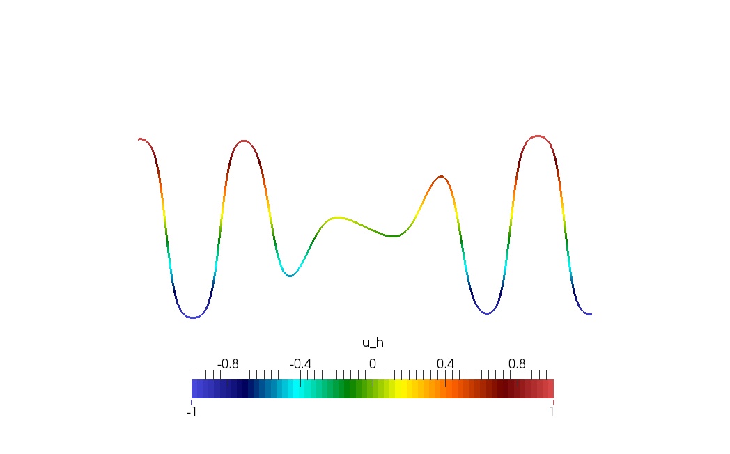
(a) $t=0.04$

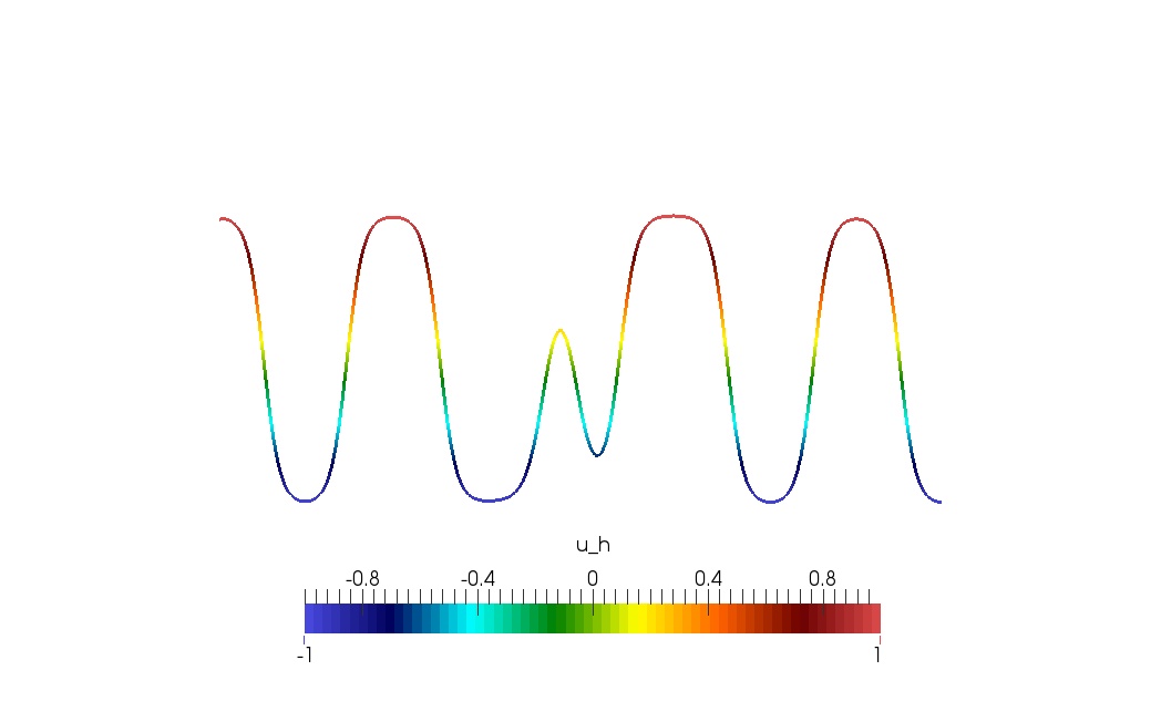
(b) $t=0.17$

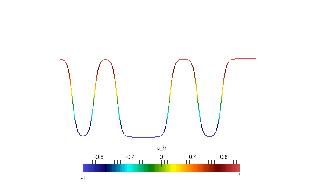
(c) $t=1.244$

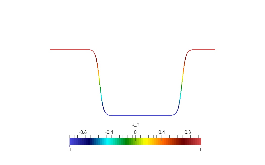
(d) $t=5$

6.3 Test 3: Test problem with non smooth initial data

In this case we benchmark an unknown solution to (2.3). We take

$$u(x,0)=\begin{cases}\frac{1}{4}\!\left({\operatorname{cos}\left(8\pi\left|x-\frac{1}{2}\right|^{2}\right)+1}\right)\text{ if }\left|x-\frac{1}{2}\right|\leq\frac{1}{8}\\ 0\text{ otherwise }\end{cases},\qquad v(x,0)\equiv 0.$$ (6.11)

The initial conditions do not satisfy the assumptions of Theorem 2.2. In fact, $u_{0}\in\operatorname{H}^{2}(\Omega)\not\ \ \operatorname{H}^{3}(\Omega)$. We summarise the results of this experiment in Table 5 and Figure 2.

Table 5: Test 3 : In this test we conduct a simulation with the initial conditions do not have the required regularity to yield a strong solution. The temporal discretisation is a $2$nd order Crank–Nicolson method and we choose $\delta t=1/N^{2}$ and $T=50$. We look at the computed estimator $\mathfrak{H}_{R}$ and its convergence. In this test we choose $\gamma=10^{-3},\mu=10^{-1}$. Note that the estimator converges at the same rates for all values of $p$. This is expected since the solution can not be $\operatorname{L}_{\infty}(0,T;\operatorname{H}^{3}(\Omega))$ which would be a strong solution. Since the estimator is an upper bound for $e_{R}$ we have that $e_{R}$ is converging, however, suboptimally for $p>1$.

$N$	$p=1$		$p=2$		$p=3$
	$\mathfrak{H}_{R}$	EOC	$\mathfrak{H}_{R}$	EOC	$\mathfrak{H}_{R}$	EOC
16	1.188578e+04	0.000	3.246291e+03	0.000	2.911743e+03	0.000
32	4.669754e+03	1.348	4.804005e+03	-0.565	4.669754e+03	-0.682
64	5.463170e+03	-0.226	4.729163e+03	0.023	4.521050e+03	0.047
128	3.766053e+03	0.537	3.270226e+03	0.532	3.241540e+03	0.480
256	2.047099e+03	0.880	1.852629e+03	0.820	1.843336e+03	0.814
512	1.046615e+03	0.968	9.555120e+02	0.955	9.534166e+02	0.951
1024	5.256529e+02	0.994	4.811709e+02	0.990	4.804343e+02	0.989

Figure 2: Test 3 : The solution, $u_{h}$ to the regularised elastodynamics system at various values of $t$.

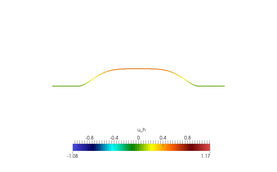
(a) $t=0.00$

(b) $t=0.1$

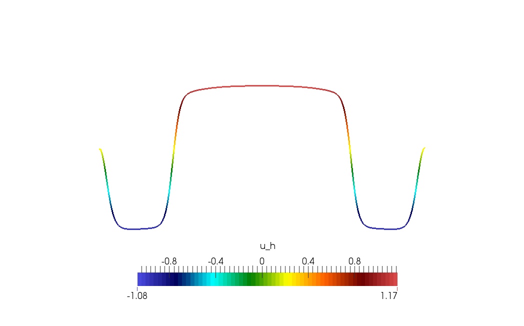
(c) $t=0.29$

(d) $t=0.5$

References

- Abeyaratne & Knowles (1991) Abeyaratne, R. & Knowles, J. K. (1991) Kinetic relations and the propagation of phase boundaries in solids. Arch. Rational Mech. Anal., 114, 119–154.
- Bona et al. (2013) Bona, J. L., Chen, H., Karakashian, O. & Xing, Y. (2013) Conservative, discontinuous Galerkin-methods for the generalized Korteweg-de Vries equation. Math. Comp., 82, 1401–1432.
- Braack & Prohl (2013) Braack, M. & Prohl, A. (2013) Stable discretization of a diffuse interface model for liquid-vapor flows with surface tension. ESAIM: Mathematical Modelling and Numerical Analysis, 47, 401–420.
- Chalons & LeFloch (2001) Chalons, C. & LeFloch, P. G. (2001) High-order entropy-conservative schemes and kinetic relations for van der Waals fluids. J. Comput. Phys., 168, 184–206.
- Cheng & Shu (2008) Cheng, Y. & Shu, C.-W. (2008) A discontinuous Galerkin finite element method for time dependent partial differential equations with higher order derivatives. Math. Comp., 77, 699–730.
- Ciarlet (2002) Ciarlet, P. G. (2002) The finite element method for elliptic problems. Classics in Applied Mathematics, vol. 40. Philadelphia, PA: Society for Industrial and Applied Mathematics (SIAM), pp. xxviii+530. Reprint of the 1978 original [North-Holland, Amsterdam; MR0520174 (58 #25001)].
- Dafermos (1979) Dafermos, C. M. (1979) The second law of thermodynamics and stability. Arch. Rational Mech. Anal., 70, 167–179.
- Dafermos (2010) Dafermos, C. M. (2010) Hyperbolic conservation laws in continuum physics. Grundlehren der Mathematischen Wissenschaften, vol. 325, third edn. Berlin: Springer-Verlag, pp. xxxvi+708.
- Diehl (2007) Diehl, D. (2007) Higher order schemes for simulation of compressible liquid–vapor flows with phase change. Ph.D. thesis, Universität Freiburg.
- DiPerna (1979) DiPerna, R. J. (1979) Uniqueness of solutions to hyperbolic conservation laws. Indiana Univ. Math. J., 28, 137–188.
- Evans (1998) Evans, L. C. (1998) Partial differential equations. Graduate Studies in Mathematics, vol. 19. Providence, RI: American Mathematical Society, pp. xviii+662.
- Georgoulis et al. (2014) Georgoulis, E. H., Hall, E. & Makridakis, C. (2014) Error control for discontinuous galerkin methods for first order hyperbolic problems. Recent Developments in Discontinuous Galerkin Finite Element Methods for Partial Differential Equations (X. Feng, O. Karakashian & Y. Xing eds). The IMA Volumes in Mathematics and its Applications, vol. 157. Springer International Publishing, pp. 195–207.
- Giesselmann et al. (2014a) Giesselmann, J., Makridakis, C. & Pryer, T. (2014a) Aposteriori analysis of discontinuous galerkin schemes for systems of hyperbolic conservation laws. Submitted - tech report availible on ArXiV.
- Giesselmann et al. (2014b) Giesselmann, J., Makridakis, C. & Pryer, T. (2014b) Energy consistent discontinuous Galerkin methods for the Navier-Stokes-Korteweg system. Math. Comp., 83, 2071–2099.
- Giesselmann (2014a) Giesselmann, J. (2014a) Low mach asymptotic-preserving scheme for the euler–korteweg model. IMA Journal of Numerical Analysis.
- Giesselmann (2014b) Giesselmann, J. (2014b) A relative entropy approach to convergence of a low order approximation to a nonlinear elasticity model with viscosity and capillarity. accepted for publication in SIAM J. Math. Anal.
- Giesselmann & Pryer (2013) Giesselmann, J. & Pryer, T. (2013) Energy mimetic discontinuous galerkin methods for a quasi incompressible phase transition model. To appear in M2AN - tech report available on ArXiV http://http://arxiv.org/abs/1307.8248.
- Giesselmann & Pryer (2014) Giesselmann, J. & Pryer, T. (2014) Reduced relative entropy techniques for apriori analysis of multiphase problems in elastodynamics. Submitted - tech report available on ArXiV.
- Jamet et al. (2001) Jamet, D., Lebaigue, O., Coutris, N. & Delhaye, J. M. (2001) The second gradient method for the direct numerical simulation of liquid-vapor flows with phase change. J. Comput. Phys., 169, 624–651.
- Jamet et al. (2002) Jamet, D., Torres, D. & Brackbill, J. (2002) On the theory and computation of surface tension: The elimination of parasitic currents through energy conservation in the second-gradient method. J. Comp. Phys, 182, 262–276.
- Karakashian & Pascal (2003) Karakashian, O. A. & Pascal, F. (2003) A posteriori error estimates for a discontinuous Galerkin approximation of second-order elliptic problems. SIAM J. Numer. Anal., 41, 2374–2399 (electronic).
- LeFloch (2002) LeFloch, P. G. (2002) Hyperbolic systems of conservation laws. Lectures in Mathematics ETH Zürich. Basel: Birkhäuser Verlag, pp. x+294. The theory of classical and nonclassical shock waves.
- Makridakis & Nochetto (2003) Makridakis, C. & Nochetto, R. H. (2003) Elliptic reconstruction and a posteriori error estimates for parabolic problems. SIAM J. Numer. Anal., 41, 1585–1594 (electronic).
- Makridakis & Nochetto (2006) Makridakis, C. & Nochetto, R. H. (2006) A posteriori error analysis for higher order dissipative methods for evolution problems. Numer. Math., 104, 489–514.
- Ortner & Süli (2007) Ortner, C. & Süli, E. (2007) Discontinuous Galerkin finite element approximation of nonlinear second-order elliptic and hyperbolic systems. SIAM J. Numer. Anal., 45, 1370–1397.
- Slemrod (1983) Slemrod, M. (1983) Admissibility criteria for propagating phase boundaries in a van der Waals fluid. Arch. Rational Mech. Anal., 81, 301–315.
- Slemrod (1984) Slemrod, M. (1984) Dynamic phase transitions in a van der Waals fluid. J. Differential Equations, 52, 1–23.
- Xu & Shu (2011) Xu, Y. & Shu, C.-W. (2011) Local discontinuous Galerkin methods for the Degasperis-Procesi equation. Commun. Comput. Phys., 10, 474–508.