Förster resonance energy transfer, absorption and emission spectra in multichromophoric systems: I. Cumulant expansions

Abstract

We study the Förster resonant energy transfer (FRET) rate in multichromophoric systems. The multichromophoric FRET rate is determined by the overlap integral of the donor’s emission and acceptor’s absorption spectra, which are obtained via 2nd-order cumulant expansion techniques developed in this work. We calculate the spectra and multichromophoric FRET rate for both localized and delocalized systems. (i) The role of the initial entanglement between the donor and its bath is found to be crucial in both the emission spectrum and the multichromophoric FRET rate. (ii) The absorption spectra obtained by the cumulant expansion method are quite close to the exact one for both localized and delocalized systems, even when the system-bath coupling is far from the perturbative regime. (iii) For the emission spectra, the cumulant expansion can give very good results for the localized system, but fail to obtain reliable spectra of the high excitations of a delocalized system, when the system-bath coupling is large and the thermal energy is small. (iv) Even though, the multichromophoric FRET rate is good enough since it is determined by the overlap integral of the spectra.

I Introduction

Background. Excitonic energy transfer (EET) Agranovich and Galanin (1982); Andrews and Demidov (1999); May and Kühn (2004); Micha and Burghardt (2007); Förster (1965) attracts extensive interest in many subjects. It is a fundamental problem in various physical and chemical processes Blankenship (2002); Renger et al. (2001); Novoderezhkin and Grondelle (2010); Varnavski et al. (2002); Nguyen et al. (2000); Bopp et al. (1999); Oijen et al. (1999); Ye et al. (2012). In general, the efficiency of the EET can be well quantified by the F rster resonance energy transfer (FRET) theory Förster (1965); Agranovich and Galanin (1982); Andrews and Demidov (1999) under the following two conditions. (a) The system can be treated as two parts: the donor and acceptor, and the coupling between them is much weaker then the system-bath coupling, i.e., the transfer is usually incoherent. (b) Both acceptor and donor can be treated as point dipoles.

However, the FRET theory is problematic in real systems such as light-harvesting complexes LH1/LH2 Bopp et al. (1999); Oijen et al. (1999), dendrimers Varnavski et al. (2002); Nguyen et al. (2000), and conjugated polymers Nguyen et al. (2000). In these systems, the donor and/or acceptor could have more than one chromophore, and cannot be treated as point dipoles. Moreover, due to the electronic couplings $V^{D}$($V^{A}$) within the donor(acceptor), the excitations are not localized, and their coherent dynamics could be quite important in the EET process Collini et al. (2010); Engel et al. (2007); Mercer et al. (2009); Lee et al. (2007); Ishizaki et al. (2010), which was shown recently in two-dimensional electronic spectroscopy experiments Abramavicius et al. (2009); Cho (2008); Jonas (2003). The energy transfer rate is significantly underestimated by the FRET theory, such as in the LH2 complex Herek et al. (2000); Hu et al. (2002); Beljonne et al. (2009). Therefore, the multichromophoric FRET theory was developed Sumi (1999); Scholes (2003); Jang et al. (2004) to solve this problem.

It should be noted that, under some experimental conditions, even the extension from the FRET to multichromophoric FRET is not enough, since they are 2nd-order theory with respect to the donor-acceptor coupling $H_{c}$. Nontrivial quantum effects such as multi-site quantum coherence and solvent-controlled transfer can be seen in higher order corrections Wu and Cao (2013).

Similar to its single chromophoric counterpart, the multichromophoric FRET rate is determined by an overlap integral between the donor’s emission and acceptor’s absorption spectra. The spectra are broadened and shifted due to the environment, which is believed to play a critical role in the EET process of light-harvesting complexes, which could achieve the order of a few picoseconds Mennucci and Curutchet (2011).Unlike the case in the FRET theory, where the spectra can be obtained exactly for an environment with Gaussian fluctuations Mukamel (1995), the spectra in the multichromophoric FRET theory are more involved, especially the emission spectrum.

I.1 Outline of this paper

Absorption and Emission spectra. In the calculation of the multichromophoric FRET rate, the absorption spectrum is relatively easier to obtain since the initial state is factorized. The emission spectrum is much more complicated due to the initial system-bath coupling, which displaces the bath away from its equilibrium. This displacement will affect the subsequent dynamics, which is reflected by a complex-time correlation function.

Donor-bath entanglement. The influence of the initial entanglement or correlation between the donor and bath is widely noticed but lack of systemic study, partially due to the difficulties in numerical techniques. Moreover, this problem does not happen in the monomer case, where the system is only one-dimensional. In this work, we find that the donor-bath entanglement plays a crucial role in both the emission spectrum and multichromophoric FRET rate. Exact numerical comparisons show the failure of two different factorization approaches for both localized and delocalized systems.

Full 2nd-order cumulant expansion. The primary goal of this series of papers is to develop analytical and numerical techniques to compute the multichromophoric FRET rate and spectra. Nonperturbative numerical methods such as stochastic path integrals Moix et al. (2013) and hierarchy equation of motions (HEOM) Tanimura (2006, 1993); Ishizaki et al. (2010); Ishizaki and Fleming (2009, 2009); Chen et al. (2009); Strümpfer and Schulten (2011); Jing et al. (2013) can give benchmarks, however, for small systems only due to the limitation of computing powers. Perturbative methods Sumi (1999); Jang and Silbey (2003); Renger and Marcus (2002); Banchi et al. (2013); Maier et al. (2011); Lee et al. (2012); Yang (2005); Zhang et al. (1998); Kolli et al. (2011); Novoderezhkin et al. (2004); Cho et al. (2005); Yang and Fleming (2002); Ohta et al. (2001); Schröder et al. (2006) are efficient for larger systems but only in some specific parameter regimes. For example, in the weak system-bath coupling regime, the EET was generally studied by using Green’s function Sumi (1999), 2nd-order time-convolution (TC2) Jang et al. (2004); Jang and Silbey (2003) and time-convolution-less (TCL2) master equations Renger and Marcus (2002); Banchi et al. (2013)

In this paper, we demonstrate the difficulties and problems in the multichromophoric FRET spectra, and focus on a perturbation approach based on the 2nd-order cumulant expansion. Here, the cumulant expansion is performed on the full system-bath coupling Hamiltonian $H_{sb}$ in both the real- and imaginary-time domains. Therefore, the absorption and emission spectra are expressed in full 2nd-order cumulant expansions (FCE), which can reduce to the exact results in the monomer case. As previously shown in the calculation of vibrational spectra Yang et al. (2004); Schröder et al. (2006), factorization of the FCE leads to further approximations that are easy to evaluate analytically. In the exciton bases $H_{sb}$ will have off-diagonal terms. If the off-diagonal part $H_{sb}^{od}$ is neglected, the FCE reduces to the inverse participation ratio (IPR) Cho et al. (2005); Cleary and Cao (2013) method. The IPR method can be improved by treating the off-diagonal elements perturbatively Yang et al. (2004); Schröder et al. (2006), and here we call this method the off-diagonal cumulant expansion (OCE). The advantage of the FCE over the OCE and IPR methods can be seen in a highly delocalized case, where the omission or perturbation treatment of the off-diagonal coupling is unreliable. For the absorption spectrum, the FCE is the same as the TCL2 in formalism, unlike the TC2 method which cannot reduce to the monomer case. For the emission spectrum, both the TCL2 and TC2 methods cannot reduce to the monomer case. The TCL2 method needs the help of a detailed balance identity to overcome this problem Banchi et al. (2013). However, the FCE is more straightforward and can reduce to the monomer case naturally.

Reliability. We use the FCE method to calculate the spectra and the multichromophoric FRET rate for both localized and delocalized systems. Firstly, for both systems, the FCE method is quite reliable in the absorption spectrum, since there is no population dynamics while the coherence decays so fast as the increase of the system-bath coupling.

For the emission spectrum, the FCE method is also quite reliable when the free excitations of the donor is localized, since the FCE is exact for monomers. However, if the donor’s free excitations are delocalized, the perturbation of the imaginary-time part is unreliable when the system’s energy gap is larger than the thermal energy. In this case, the emission spectrum is still reliable if it is determined by the lower excited states. The multichromophoric FRET rates of the two systems are still close to the exact one since the rate is determined by the spectra overlap.

This paper is organized as follows. In Sec. II we give the physical model of a multichromophoric system and introduce the multichromophoric FRET theory. The role of the initial entanglement is showed by using the HEOM method. In Sec. III we derive the absorption and emission spectra by using 2nd-order cumulant expansion techniques. We find that the spectra formula can be further simplified when the system has translational symmetry. Then we calculate the spectra and multichromophoric FRET rate for localized and delocalized systems, and discuss the reliability of the cumulant expansion method.

I.2 Outline of the forth-coming papers

We find that the limitation of the FCE method, as well as many other traditional perturbation methods, lies in the emission spectrum of a delocalized system in the low-temperature and large system-bath coupling regimes. To overcome this problem, several new methods are developed in our group and will appear as a sequel.

(a) For real systems such as the LH2, the energy gaps of the first excitations are comparable to both the thermal energy and the system-bath coupling. All the traditional perturbation methods cannot give reliable emission spectrum and the multichromophoric FRET rate. For such systems, the treatments of the complex-time system-bath correlation will determine the reliability of the emission spectrum and the multichromophoric FRET rate. In our Paper II Ma et al. (2013), we develop a hybrid cumulant expansion method, which uses the imaginary-time path integrals to obtain the exact reduced density matrix of the donor, from which the displacements of the bath operators can be extracted more precisely. Using this method, we can give reliable emission spectrum and multichromophoric FRET rate of the LH2 system Moix et al. (2013).

(b) If the system-bath coupling is dominant, even when the donor’s free excitations are delocalized, perturbation should be made on the donor’s off-diagonal coupling $V$ but not the system-bath coupling. This O($V^{2}$) expansion is developed in our paper III Cleary and Cao (2013).

(c) Furthermore, to overcome the problems of the HEOM in calculating large system and low temperature conditions, in our Paper IV Moix et al. (2013) we implement a complex-time stochastic PI method, which will be our benchmarks.

II Multichromophoric FRET Theory

II.1 Model Hamiltonian

The multichromophoric FRET theory describes the resonant energy transfer between a donor (D) and an acceptor (A) in an multichromophoric system, described by the Hamiltonian

$$H=H_{t}^{D}+H_{t}^{A}+H_{c},$$ (1)

where $H_{c}$ is the dipole-dipole coupling between the donor and acceptor, and $H_{t}^{D(A)}$ is the total Hamiltonian of the donor (acceptor) and its bath,

$$H_{t}^{D} = H_{s}^{D}+H_{sb}^{D}+\mathbb{I}_{s}^{D}H_{b},$$

$$H_{t}^{A} = H_{s}^{A}+H_{sb}^{A}+\mathbb{I}_{s}^{A}H_{b}.$$ (2)

We first explain the donor’s part. The free Hamiltonian of the donor is

$$H_{s}^{D}\!\!\! =\!\!\! \sum_{m=1}^{N_{D}}\!\left(\epsilon_{m}^{D}\!+\lambda_{m}^{D}\right)\!\!|D_{m}\rangle\langle D_{m}|\!+\!\sum_{m\neq n}^{N_{D}}\!V_{mn}^{D}|D_{m}\rangle\langle D_{n}|$$ (3)

where $\epsilon_{m}^{D}$ is the excitation energy of the donor’s $m$th site, and $\lambda_{m}^{D}$ is the reorganization energy induced by the interaction between the bath and the donor’s $m$th chromophore. $V_{mn}^{D}$ is the coupling between sites $m$ and $n$. In the multichromophoric FRET theory, we focus on the single excitation case and thus $|D_{m}\rangle$ represents the state that the total multichromophoric system is excited only at the donor’s $m$th site, all the other sites (including the acceptor’s) are in their ground states, i.e.,

$$|D_{m}\rangle=|0,\dots 1_{m},\dots,0\rangle_{D}|0\dots 0\rangle_{A}.$$ (4)

The identity operator $\mathbb{I}_{s}^{D}$ is given by

$$\mathbb{I}_{s}^{D}=\sum_{m=1}^{N_{D}}|D_{m}\rangle\langle D_{m}|.$$ (5)

In this work, the baths that couple to different chromophores are independent. Therefore, it is convenient to write the free Hamiltonian of the bath as $H_{b}=H_{b}^{D}+H_{b}^{A}$, and then we can write the total Hamiltonians as

$$H_{t}^{D} =H^{D}+\mathbb{I}_{s}^{D}H_{b}^{A},$$

$$H_{t}^{A} =H^{A}+\mathbb{I}_{s}^{A}H_{b}^{D},$$ (6)

which will be used in the following content. The correlated bath was studied in Ref. Wu et al. (2010); Strümpfer and Schulten (2011). The bath is usually modeled by a set of harmonic oscillators,

$$H_{b}^{D}=\sum_{m=1}^{N_{D}}\sum_{k}\hbar\omega_{m,k}^{D}b_{m,k}^{D\dagger}b_{m,k}^{D},$$ (7)

where $\omega_{m,k}^{D}$ is the frequency of the $k$th mode of the bath that coupled with the $m$th site of the donor(acceptor). The excitation states couple with the harmonic bath linearly as

$$H_{sb}^{D} = \sum_{m=1}^{N_{D}}\hat{B}_{m}^{D}|D_{m}\rangle\langle D_{m}|,$$ (8)

where the bath operators are given by

$$\hat{B}_{m}^{D} = \sum_{k}g_{m,k}^{D}\left(b_{m,k}^{D\dagger}+b_{m,k}^{D}\right).$$ (9)

The relation between the coupling strengths $g_{m,k}^{D}$ and the reorganization energy is $\lambda_{m}^{D}\equiv\sum_{k}g_{m,k}^{2}/\omega_{m,k}$.

The acceptor’s Hamiltonians $H_{s}^{A}$, $H_{b}^{A}$ and $H_{sb}^{A}$ are obtained by replacing the notation $D$ with $A$ in the above discussion.

The dipole-dipole interaction between the donor and acceptor is given by

$$H_{c}=\sum_{m=1}^{N_{D}}\sum_{n=1}^{N_{A}}J_{mn}\left(|D_{m}\rangle\langle A_{n}|+\text{$|A_{n}\rangle\langle D_{m}|$}\right),$$ (10)

where the couplings $J_{mn}$ are treated perturbatively in the multichromophoric FRET theory.

II.2 Gold-rule formulation of the multichromophoric FRET rate

Before the study of the multichromophoric FRET rate $k$, we should understand the time scales in the energy transfer process. The multichromophoric FRET theory describes the incoherent transfer of excitations from a donor to an acceptor. This transfer happens after the donor is excited to its first excitation states. In general, the donor’s initial excitations will relax to an equilibrium state with its bath in a time scale that is much shorter than the excitation transfer time $1/k$. Therefore, the initial condition of the multichromophoric FRET process can be considered as an equilibrium state of the donor and its bath. On the other hand, the lifetime of the first excitations are usually much longer than the excitation transfer time, and thus the ground state is not involved in the multichromophoric FRET theory.

Based on the above conditions, the multichromophoric FRET rate can be derived straightforwardly from the Fermi’s golden rule Sumi (1999),

$$k=2\pi\sum_{\mu\nu}P_{\nu}^{D}\left|\langle\Psi_{\nu}^{D}|H_{c}|\Phi_{\mu}^{A}\rangle\right|^{2}\delta\left(E_{\nu}^{D}-E_{\mu}^{A}\right),$$ (11)

where $|\Psi_{\nu}^{D}\rangle$ ($|\Phi_{\mu}^{A}\rangle$) and $E_{\nu}^{D}$ ($E_{\mu}^{A}$) are the eigenstates and eigenenergies of $H_{t}^{D}$ ($H_{t}^{A}$), which include the degrees of freedom of both the system and bath. $P_{\nu}^{D}$ is obtained from

$$\rho^{D}=\rho_{e}^{D}\rho_{b}^{A}=\sum_{\nu}P_{\nu}^{D}|\Psi_{\nu}^{D}\rangle\langle\Psi_{\nu}^{D}|,$$ (12)

where

$$\rho_{e}^{D}=\frac{e^{-\beta H^{D}}}{\text{tr}e^{-\beta H^{D}}},\;\rho_{b}^{A}=\frac{e^{-\beta H_{b}^{A}}}{\text{tr}e^{-\beta H_{b}^{A}}},$$ (13)

and $\beta=k_{B}T$, with $k_{B}$ the Boltzmann’s constant and $T$ the temperature.

Starting from Eq. (11), the multichromophoric FRET rate can be derived as

$$k= \sum_{m,n}\sum_{m^{\prime}n^{\prime}}J_{mn}J_{m^{\prime}n^{\prime}}\int_{-\infty}^{\infty}dt\,\text{tr}_{b}\big{\{}e^{iH_{t}^{D}t}\rho_{e}^{D}\rho_{b}^{A}$$ (14)

$$\times|D_{m^{\prime}}\rangle\langle A_{n^{\prime}}|e^{-iH_{t}^{A}t}|A_{n}\rangle\langle D_{m}|\big{\}},$$

where the degrees of freedom of the acceptor and donor can be treated separately as

$$k =\sum_{m,n}\sum_{m^{\prime}n^{\prime}}J_{mn}J_{m^{\prime}n^{\prime}}\int_{-\infty}^{\infty}dt\,$$

$$\times\text{tr}_{bA}\left[\rho_{b}^{A}e^{iH_{b}^{A}t}\langle A_{n^{\prime}}|e^{-iH^{A}t}|A_{n}\rangle\right]$$

$$\times\text{tr}_{bD}\left[\langle D_{m}|e^{iH^{D}t}\rho_{e}^{D}|D_{m^{\prime}}\rangle e^{-iH_{b}^{D}t}\right].$$ (15)

Now we can define two matrices

$$\mathbf{I}^{A}\left(t\right) = \text{tr}_{b}\left(e^{-iH^{A}t}\rho_{b}^{A}e^{iH_{b}^{A}t}\right),$$ (16)

$$\mathbf{E}^{D}\left(t\right) = \text{tr}_{b}\left(e^{iH^{D}t}\rho_{e}^{D}e^{-iH_{b}^{D}t}\right),$$ (17)

and the multichromophoric FRET rate can be expressed as

$$k = \int_{-\infty}^{\infty}dt\,\text{tr}\left[\mathbf{J}^{T}\mathbf{E}^{D}\left(t\right)\mathbf{J}\mathbf{I}^{A}\left(t\right)\right],$$ (18)

where

$$\mathbf{J}=\sum J_{mn}|D_{m}\rangle\langle A_{n}|.$$ (19)

It is important to notice that the density matrix in $\mathbf{I}^{A}\left(t\right)$ is the thermal equilibrium state of the acceptor’s bath. The donor is assumed to be in its excited equilibrium state $\rho_{e}^{D}$. This non-factorized initial state brings technique difficulties in the calculation of emission spectrum, especially when the system-bath coupling is strong. The primary goal of this series of papers is to develop analytical and numerical techniques to compute the donor-bath correlations.

The absorption and emission spectra are given by

$$\mathbf{I}^{A}\left(\omega\right) = \int_{-\infty}^{\infty}dt\,e^{i\omega t}\mathbf{I}^{A}\left(t\right),$$

$$\mathbf{E}^{D}\left(\omega\right) = \int_{-\infty}^{\infty}dt\,e^{-i\omega t}\mathbf{E}^{D}\left(t\right),$$ (20)

and thus the multichromophoric FRET rate can also be written as Sumi (1999); Jang et al. (2004)

$$k=\frac{1}{2\pi}\int_{-\infty}^{\infty}d\omega\,\text{tr}\left[\mathbf{J}^{T}\mathbf{E}^{D}\left(\omega\right)\mathbf{J}\mathbf{I}^{A}\left(\omega\right)\right].$$ (21)

From the above formula, the rate $k$ is determined by the donor-acceptor coupling $\mathbf{J}$, and the overlap integral of the acceptor’s absorption spectrum $\mathbf{I}_{nn^{\prime}}^{A}\left(\omega\right)$ and the donor’s emission spectrum $\mathbf{E}_{m^{\prime}m}^{D}\left(\omega\right)$. The influences of the system-bath coupling on the transfer rate are reflected by the spectra in their widths and positions, which are determined by the relaxation dynamics and reorganization energies, respectively. Therefore, the main problem here is to calculate the spectra. We should note that the spectra (20) in the multichromophoric FRET rate do not depend on the system’s local dipoles. Actually, the commonly studied far-field spectra $I_{\text{f}}^{A}\left(\omega\right)$ and $E_{\text{f}}^{D}\left(\omega\right)$ can be obtained as

$$I_{\text{f}}^{A}\left(\omega\right) =\sum_{m,n}\left(\hat{\epsilon}\cdot\vec{\mu}_{m}^{A}\right)\left(\hat{\epsilon}\cdot\vec{\mu}_{n}^{A}\right)\,I_{mn}^{A}\left(\omega\right),$$

$$E_{\text{f}}^{D}\left(\omega\right) =\sum_{m,n}\left(\hat{\epsilon}\cdot\vec{\mu}_{m}^{D}\right)\left(\hat{\epsilon}\cdot\vec{\mu}_{n}^{D}\right)\,E_{mn}^{D}\left(\omega\right),$$ (22)

where $\hat{\epsilon}$ is the polarization of the light and $\vec{\mu}_{i}$ denote the local dipole operators.

In this work, for the sake of simplicity, the donor-acceptor coupling is $J_{mn}=J$. Therefore, the multichromophoric FRET rate formula (21) can be simplified as

$$k=\frac{J^{2}}{2\pi\hbar^{2}}\int_{-\infty}^{\infty}d\omega E^{D}\left(\omega\right)I^{A}\left(\omega\right),$$ (23)

where

$$E^{D}\left(\omega\right) = \sum_{m,n}E_{mn}^{D}\left(\omega\right),$$

$$I^{A}\left(\omega\right) = \sum_{m,n}I_{mn}^{A}\left(\omega\right).$$ (24)

III Effects of donor-bath entanglement

In the multichromophoric FRET theory, the donor is first excited to its single-excitation subspace, which becomes equilibrium with its bath in a time scale that is negligibly small as compared with the EET time. Therefore, the initial state is an equilibrium state of the donor and its bath, as shown in Eq. (17). In this case, the donor and its bath are usually correlated or entangled due to their interaction, which is characterized by the reorganization energy $\lambda$.

When $\lambda$ is smaller than the system’s energy scale, or the bath correlation time is negligibly small (e.g. in the high-temperature limit), the Born approximation is employed and a master equation is obtained. However, when the system-bath interaction is larger than the other energy scales, the Born approximation is invalid, and the system and bath are non-factorized during the entire multichromophoric FRET process. To our knowledge, only a few methods can treat the system-bath correlation exactly. Here we first use the HEOM method to show the crucial role of the donor-bath entanglement. The 2nd-order correction of the initial state was studied in Sec. IV B.

In this work, the donor and acceptor each consists of two chromophores. Since the entanglement relies on the properties of the system, we consider two limiting cases. In the Case I, the system is localized, and its Hamiltonian is (in the unit of $\text{cm}^{-1}$)

$$H_{s}^{D1}=\begin{pmatrix}250&20\\ 20&150\end{pmatrix},\;H_{s}^{A1}=\begin{pmatrix}100&20\\ 20&0\end{pmatrix},$$ (25)

where the ratio of the excitation energy difference $\Delta=E_{2}-E_{1}$ and the inter-chromophore coupling $V$ is $\Delta/V=5$. In the Case II, the system is delocalized ($\Delta/V$=0.2),

$$H_{s}^{D2}=\begin{pmatrix}200&100\\ 100&180\end{pmatrix},\;H_{s}^{A2}=\begin{pmatrix}100&100\\ 100&80\end{pmatrix}.$$ (26)

The influence of the bath on the system dynamics is determined by the system-bath coupling spectrum, here we choose the Drude spectrum

$$J\left(\omega\right)=\frac{2\lambda\omega\gamma}{\omega^{2}+\gamma^{2}},$$ (27)

where $\lambda$ is the reorganization energy and $\gamma$ is the cutoff frequency of the bath. For the sake of simplicity, the reorganization energies are the same for each site. The donor-acceptor coupling is $J_{mn}=J=10\,\text{cm}^{-1}$.

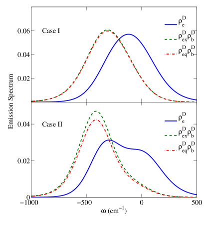
Figure 1: Comparison of emission spectra for different initial state in localized (Case I) and delocalized (Case II) systems. The reorganization energy $\lambda=100\,\text{cm}^{-1}$, the cutoff frequency $\gamma=10\,\text{ps}^{-1}$, and the temperature $T=300\,\text{K}$.

To study the effects of the initial entanglement, we consider three different treatments of the initial state:

(i) The initial state is obtained exactly by using HEOM. In this case, the system and bath first evolved to equilibrium, and the correlation information between system and bath is carried by the auxiliary fields of the HEOM. Then the system and bath evolve according to Eq. (17). The emission spectrum obtained in this case is exact Jing et al. (2013).

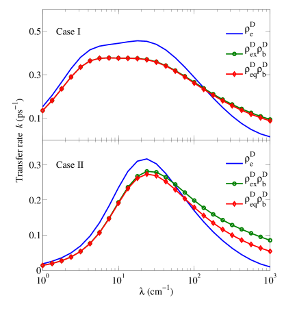
Figure 2: Comparison of multichromophoric FRET rate as a function of reorganization energy $\lambda$ from $1\,\text{cm}^{-1}$ to $1000\,\text{cm}^{1}$ for different initial states. All the other parameters are the same as in Fig. 1.

(ii) The initial state is factorized, but the system’s reduced density matrix is exact,

$$\rho\left(0\right)=\rho_{\text{ex}}^{D}\rho_{b}^{D},$$ (28)

where $\rho_{\text{ex}}^{D}$ is the exact reduced density matrix of the donor, and $\rho_{b}^{D}=\exp\left(-\beta H_{b}^{D}\right)/Z_{b}^{D}$ is the equilibrium state of the bath. In this case, we use the HEOM method to obtain the exact reduced density matrix, then all the auxiliary fields are reset to be zeros. Thus the correlation between system and bath is turned off. Alternatively, we can obtain the reduced density matrix directly using the imaginary-time path integral method Moix et al. (2012).

(iii) The initial state is also factorized as

$$\rho\left(0\right)=\rho_{\text{eq}}^{D}\rho_{b}^{D},$$ (29)

however, $\rho_{\text{eq}}^{D}=\exp\left(-\beta H_{s}^{D}\right)/Z_{s}^{D}$ is the thermal equilibrium state of donor. This is also the initial state commonly used in master equation method.

Comparison of emission spectra $E^{D}\left(\omega\right)$ for different initial states are shown in Fig. 1. Because the reorganization energy $\lambda=100\,\text{cm}^{-1}$ is comparable to the excitation energies, thus the separable approximation is not reliable. For the localized system (Case I), the spectra obtained by separable approximation are shifted due to the ignore of reorganization. The delocalized system (Case II) is more interesting, where the double-peak structure disappears in the approximate spectra. The entanglement effect in the delocalized case is more notable than in the localized one. We consider a limiting case, the system is fully localized, i.e., the intermolecular coupling $V=0$, thus the chromophores are independent, and there is no entanglement between the donor and its bath. Actually, in this case the initial state can be written as

$$\rho\left(0\right)=\rho_{\text{eq}}^{D}\tilde{\rho}_{b}^{D},$$ (30)

where $\tilde{\rho}_{b}^{D}$ is the equilibrium state of the displaced bath.

The effects of initial entanglement on multichromophoric FRET rate is shown in Fig. 2. For both the localized and delocalized cases, the factorized initial state approximation breaks down rapidly with the increase of system-bath coupling. It is interesting to note that, in the delocalized case (lower panel) the multichromophoric FRET rates obtained from $\rho_{\text{ex}}^{D}\rho_{b}^{D}$ and $\rho_{\text{eq}}^{D}\rho_{b}^{D}$ differ dramatically for very large $\lambda$, which reflects the deviation of $\rho_{\text{ex}}^{D}$ and $\rho_{\text{eq}}^{D}$. As the entanglement plays such a notable role, we should treat the initial state in a more accurate way, such as the cumulant expansion method used below.

IV Second-order Cumulant expansion

In this section we derive the cumulant expansion formulas of the absorption and emission spectra. The absorption and emission spectra were studied by various methods, such as the standard TC2 Jang and Silbey (2003) and TCL2 Banchi et al. (2013). The TC2 method is time-nonlocal, and it cannot give reliable results even for monomers. The TCL2 method is time-local. In the monomer case, the absorption spectrum given by the TCL2 is exact. However, in this framework the TCL2 of the emission spectrum has an inhomogeneous term that describes the unfactorized initial states, and it cannot give the exact results in the monomer limit. A detailed balance identity should be used to overcome this problem Banchi et al. (2013). The cumulant expansion method shown below is similar to the TCL2 method. They give the same results for the absorption spectrum. For the emission spectrum, the cumulant expansion method can reduce to the monomer case directly, without additional terms.

IV.1 Absorption spectrum – Full 2nd-order cumulant expansion

Below, we derive the absorption spectrum via 2nd-order cumulant expansion. It is convenient to diagonalize the acceptor’s Hamiltonian $H_{s}^{A}$ at first,

$$H_{s}^{A}=\sum_{\mu=1}^{N_{A}}\epsilon_{\mu}^{A}|\mu\rangle\langle\mu|,$$ (31)

where $\epsilon_{\mu}^{A}$ is the eigenenergy (containing $\lambda$),

$$|\mu\rangle=\sum_{i=1}^{N_{A}}c_{i}^{\mu}|A_{i}^{e}\rangle,$$ (32)

is the energy eigenstate, and $c_{i}^{\mu}=\langle\mu|A_{i}^{e}\rangle$. However, in the energy representation the system-bath coupling has off-diagonal terms,

$$H_{sb}^{A}=\sum_{\mu,\nu=1}^{N_{A}}\tilde{B}_{\mu\nu}^{A}|\mu\rangle\langle\nu|,$$ (33)

where

$$\tilde{B}_{\mu\nu}^{A}=\sum_{n=1}^{N_{A}}X_{n}^{\mu\nu}B_{n}^{A}$$ (34)

and the coefficient $X_{n}^{\mu\nu}=c_{n}^{\mu}c_{n}^{\nu}$. Below, we perform cumulant expansion with respect to $H_{sb}^{A}$. In Ref. Yang et al. (2004); Schröder et al. (2006), the cumulant expansion was carried out with respect to the off-diagonal terms of the Hamiltonian $H_{sb}^{A}$ (33), which could yield unreliable results in highly delocalized cases.

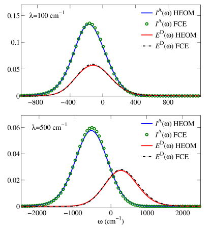
Figure 3: Absorption and emission spectra of the localized system [Case I defined in (25)]. Results are obtained by using full 2nd-order cumulant expansion (FCE) and hierarchy equation of motion (HEOM) methods. The bath parameters are the same as in Fig. 1. Even for a very large reorganization energy $\lambda=500\,\text{cm}^{-1}$, the FCE results are in very good agreement with the exact one.

The 2nd-order cumulant of $H_{sb}^{A}$ of Eq. (16) gives

$$\mathbf{I}^{A}\left(t\right) \simeq e^{-iH_{s}^{A}t}e^{-\mathbf{K}\left(t\right)},$$ (35)

where the time-dependent matrix

$$\mathbf{K}\left(t\right) = \!\int_{0}^{t}\!\!dt_{2}\int_{0}^{t_{2}}\!\!\!dt_{1}\text{tr}_{b}\left[H_{sb}^{A}\left(t_{2}\right)H_{sb}^{A}\left(t_{1}\right)\rho_{b}^{A}\right]$$ (36)

$$= \sum_{\mu,\nu=1}^{N_{A}}|\mu\rangle\langle\nu|\sum_{\alpha=1}^{N_{A}}\sum_{n=1}^{N_{A}}X_{n}^{\mu\alpha}X_{n}^{\alpha\nu}$$

$$\times\!\int_{0}^{t}\!\!dt_{2}\int_{0}^{t_{2}}\!\!\!dt_{1}e^{i\omega_{\mu\alpha}t_{2}-i\omega_{\nu\alpha}t_{1}}C_{n}^{B}\left(t_{2}\!-t_{1}\!\right),$$

where $\omega_{ij}\equiv\epsilon_{i}-\epsilon_{j}$ and

$$H_{sb}^{A}\left(t\right)\equiv e^{i\left(H_{s}^{A}+H_{b}^{A}\right)t}H_{sb}^{A}e^{-i\left(H_{s}^{A}+H_{b}^{A}\right)t}.$$ (37)

The time-correlation function of the bath $C_{n}^{B}\left(t_{2}-t_{1}\right)\equiv\text{tr}_{b}\left[B_{n}^{A}\left(t_{2}\right)B_{n}^{A}\left(t_{1}\right)\rho_{b}^{A}\right]$ is time translational invariant. In a general case if we have a complex time $\theta=s-i\tau$, the correlation function can be expressed as

$$C_{n}^{B}\left(\theta\right) = \int_{0}^{\infty}\frac{d\omega}{\pi}J_{n}\left(\omega\right)\frac{\cosh\left[\omega\left(\frac{1}{2}\beta-i\theta\right)\right]}{\sinh\left[\frac{1}{2}\omega\beta\right]},$$ (38)

where $J_{n}\left(\omega\right)$ is the coupling spectrum between the $n$th site and its bath. In this paper, we choose the Drude spectrum (27), and assume the reorganization energies are the same for different baths, i.e., $J\left(\omega\right)=J_{n}\left(\omega\right)$.

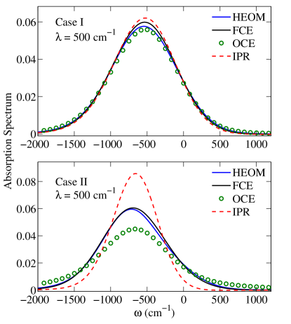
Figure 4: Absorption spectra obtained via the hierarchy equation of motion (HEOM), full 2nd-order cumulant expansion (FCE), off-diagonal cumulant expansion (OCE) and inverse participation ratio (IPR) methods. The OCE and IPR methods fail to give reliable results in delocalized case.

The calculation of the absorption spectra $I_{A}\left(\omega\right)$ for localized (25) and delocalized (26) systems are shown in Figs. 3 and 5, respectively. We know that if the system is fully localized, i.e., $V_{ij}^{D\left(A\right)}=0$, the cumulant expansion method is exact. Since the Hamiltonian (25) does not deviate from the fully localized case very much, the cumulant expansion method could give very precise results, as shown in Fig. 3. The cumulant expansion results for the delocalized system are also in good agreement with the exact spectra obtained by the HEOM method, even for a very large reorganization energy $\lambda=500\,\text{cm}^{-1}$.

IV.2 Absorption spectrum – Further approximation of the FCE method

In general, $\mathbf{K}\left(t\right)$ in Eq. (36) is a matrix, and Eq. (35) should be evaluated numerically. In a previous study of vibrational spectra Yang et al. (2004), we arrived at a similar expression and factorized the contribution from the diagonal and off-diagonal parts of the interaction Hamiltonian

$$H_{sb}^{A}=H_{sb}^{A,d}+H_{sb}^{A,od},$$ (39)

in the exciton bases, where $H_{sb}^{A,d}$ and $H_{sb}^{A,od}$ are the diagonal and off-diagonal parts. If we neglect $H_{sb}^{A,od}$ and perform cumulant expansion on the diagonal part $H_{sb}^{A,d}$ only, we will arrive at the IPR method Cleary and Cao (2013); Cleary et al. (2013), and the absorption spectrum is calculated as

$$\mathbf{I}_{IPR}^{A}\left(t\right) \simeq\sum_{\mu}|\mu\rangle\langle\mu|\exp\left[-i\epsilon_{\mu}^{A}t-K_{\mu\mu}^{IPR}\left(t\right)\right],$$ (40)

where

$$K_{\mu\mu}^{IPR}\left(t\right) =\sum_{n=1}^{N_{A}}\left|X_{n}^{\mu\mu}\right|^{2}\int_{0}^{t}\!\!dt_{2}\int_{0}^{t_{2}}\!\!\!dt_{1}C^{B}\left(t_{2}\!-t_{1}\!\right).$$ (41)

We should note that, $K_{\mu\mu}^{IPR}\left(t\right)$ is not the diagonal part of $\mathbf{K}\left(t\right)$ in Eq. (36). It is reliable only for localized case, in which the off-diagonal terms of the system-bath coupling is small. Further improvement can be made by including the contribution from $H_{sb}^{A,od}$. Actually, the diagonal part of $\mathbf{K}\left(t\right)$ can be written as

$$K_{\mu\mu}\left(t\right)=K_{\mu\mu}^{IPR}\left(t\right)+\sum_{\alpha}R_{\mu\alpha\alpha\mu}\left(t\right),$$ (42)

where

$$R_{\mu\alpha\alpha\mu}\left(t\right) =\sum_{\alpha\neq\mu}\sum_{n=1}^{N_{A}}\left(X_{n}^{\mu\alpha}\right)^{2}$$

$$\times\int_{0}^{t}\!\!dt_{2}\int_{0}^{t_{2}}\!\!\!dt_{1}e^{i\omega_{\mu\alpha}\left(t_{2}-t_{1}\right)}C\left(t_{2}-t_{1}\right)$$ (43)

reflects the transition from state $\alpha$ to $\mu$, which is induced by the off-diagonal part of the acceptor-bath interaction Hamiltonian $H_{sb}^{A,od}$. In the long time limit, $R_{\mu\alpha\alpha\mu}\equiv R_{\mu\alpha\alpha\mu}\left(\infty\right)$ is the population transfer rate. Therefore, the absorption spectrum can also be given as

$$\mathbf{I}_{OCE}^{A}\left(t\right)\simeq\sum_{\mu} |\mu\rangle\langle\mu|\exp\bigg{[}-i\epsilon_{\mu}^{A}t-K_{\mu\mu}^{IPR}\left(t\right)$$

$$-\sum_{\alpha\neq\mu}R_{\mu\alpha\alpha\mu}t\bigg{]},$$ (44)

which is named as the OCE approach. We compare these methods in Fig. 4. For localized system, all of them give reliable results. For delocalized case, since the off-diagonal terms of $H_{sb}^{D(A)}$ are not negligible, only the FCE can give reliable spectra.

IV.3 Emission spectrum

The emission spectrum is also derived in the energy representation. The density matrix $\rho_{e}^{D}$ in Eq. (17) needs to be treated carefully. We first consider the partition function $Z_{e}^{D}=\text{tr}\left(e^{-\beta H^{D}}\right)$, which is obtained by cumulant expansions

$$Z_{e}^{D} \simeq Z_{b}^{D}\text{tr}_{D}\left[e^{-\beta H_{s}^{D}}e^{\mathbf{K}^{II}\left(\beta\right)}\right],$$ (45)

where the matrix

$$\mathbf{K}^{II}\left(\beta\right) =\int_{0}^{\beta}\!\!d\tau_{2}\int_{0}^{\tau_{2}}\!\!\!d\tau_{1}\text{tr}_{b}\left[H_{sb}^{D}\!\!\left(-i\tau_{2}\right)H_{sb}^{D}\!\!\left(-i\tau_{1}\right)\rho_{b}^{D}\right]$$ (46)

$$=\sum_{\mu\nu\alpha}\sum_{n}X_{n}^{\mu\alpha}X_{n}^{\alpha\nu}|\mu\rangle\langle\nu|$$

$$\times\int_{0}^{\beta}d\tau^{\prime}e^{\omega_{\mu\nu}\tau^{\prime}}\int_{0}^{\tau^{\prime}}d\tau\,e^{\omega_{\nu\alpha}\tau}C^{B}\left(-i\tau\right),$$

and the imaginary time bath correlation function $C^{B}\left(-i\tau\right)$ is given by Eq. (38). After similar algebra used in the previous section, we obtain

$$\mathbf{E}_{D}\left(t\right)\simeq\frac{e^{-\left(\beta+it\right)H_{s}^{D}}e^{-\mathbf{K}^{RR}\left(t,\beta\right)+i\mathbf{K}^{RI}\left(t,\beta\right)+\mathbf{K}^{II}\left(\beta\right)}}{\text{tr}_{D}\left[e^{-\beta H_{s}^{D}}e^{\mathbf{K}^{II}\left(\beta\right)}\right]},$$ (47)

where

$$\mathbf{K}^{RR}\left(t,\beta\right) = \!\!\int_{0}^{t}\!\!\!ds_{2}\int_{0}^{s_{2}}\!\!\!ds_{1}\text{tr}_{b}\left[H_{sb}^{D}\!\!\left(s_{2}\!\!-\!\!i\beta\right)H_{sb}^{D}\!\!\left(s_{1}\!\!-\!\!i\beta\right)\rho_{b}^{D}\right]$$ (48)

$$= \sum_{\mu\nu\alpha}\sum_{n}X_{n}^{\mu\alpha}X_{n}^{\alpha\nu}|\mu\rangle\langle\nu|e^{\beta\omega_{\mu\nu}}$$

$$\times\int_{0}^{t}\!\!\!ds^{\prime}\,e^{i\omega_{\mu\nu}s^{\prime}}\int_{0}^{s^{\prime}}\!\!\!\!ds\,e^{i\omega_{\nu\alpha}s}\,C^{B}\left(s\right),$$

and

$$\mathbf{K}^{RI}\left(t,\beta\right) = \!\!\int_{0}^{t}\!\!\!ds\int_{0}^{\beta}\!\!\!d\tau\text{tr}_{b}\left[H_{sb}^{D}\!\!\left(s\!-\!i\beta\right)H_{sb}^{D}\!\!\left(-i\tau\right)\rho_{b}^{D}\right]$$ (49)

$$= \sum_{\mu\nu\alpha}\sum_{n}X_{n}^{\mu\alpha}X_{n}^{\alpha\nu}|\mu\rangle\langle\nu|e^{\beta\omega_{\mu\alpha}}$$

$$\times \int_{0}^{t}\!\!\!ds\int_{0}^{\beta}\!\!\!\,d\tau e^{i\omega_{\mu\alpha}s-\omega_{\nu\alpha}\tau}C^{B}\!\left(-s\!-\!i\tau\right).$$

We note that matrices $\mathbf{K}^{RR}\left(t,\beta\right)$ and $\mathbf{K}^{RI}\left(t,\beta\right)$ depend both on time and temperature, which reflect that the dynamics is affected by the initial system-bath correlation. The explicit forms of the above matrices for the Drude spectrum are given in Appendix A.

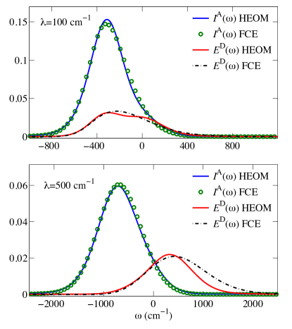
Figure 5: Absorption and emission spectra of the delocalized system (26). We compare the results of the full 2nd-order cumulant expansion (FCE) and hierarchy equation of motion (HEOM) methods. The bath parameters are the same as in Fig. 1.

The comparisons of the emission spectra $E^{D}\left(\omega\right)$ for localized [Case I (25)] and delocalized [Case II (26)] systems are shown in Figs. 3 and 5, respectively. For a localized system, the donor and its bath is just weakly entangled, thus the cumulant expansion method performs very well, as shown in Fig. 3. For a delocalized system, the donor and its bath could be strongly entangled. The emission spectra deviate from the exact one when the system-bath coupling becomes so strong that the initial state is far from a factorized state. Actually, perturbative methods are unreliable in this parameter regime. The reliability of the cumulant expansion method will be discussed in Sec. III D.

IV.4 Systems with translational symmetry

To calculate the emission and absorption spectra, we need to diagonalize all the matrices $\mathbf{K}$ in every time step according to Eqs. (35) and (47). This could be time consuming if the practical system is large. Fortunately, it can be proved that the matrices $\mathbf{K}$ are diagonal when a system has translational symmetry (the reorganization energies are also equal).

All the matrices $\mathbf{K}$ has the factor

$$\sum_{n}X_{n}^{\mu\alpha}X_{n}^{\alpha\nu}=\sum_{n}\langle\mu|n\rangle\left|\langle n|\alpha\rangle\right|^{2}\langle n|\nu\rangle.$$ (50)

If the system has translational symmetry, then

$$\left|\langle n|\alpha\rangle\right|^{2}=\left|\langle n+k|\alpha\rangle\right|^{2}=\text{const.}$$ (51)

and

$$\sum_{n}X_{n}^{\mu\alpha}X_{n}^{\alpha\nu}=\left|\langle n|\alpha\rangle\right|^{2}\delta_{\mu\nu}.$$ (52)

Therefore, all the off-diagonal terms are zero.

Usually, real systems do not have perfect translational symmetries, but have some defects or static disorders. In such cases the system can be described by $H_{0}$, which has perfect translational symmetry, plus $\delta V$, which breaks this symmetry. If $\delta V$ can be treated as a perturbation, it is easy to show that the off-diagonal terms of $\mathbf{K}$ is of order $O\left(\delta V^{4}\right)$, and can be omitted safely.

IV.5 Reliability of the cumulant expansion for the emission spectrum

The emission spectra shown in Fig. 5 indicate that the cumulant expansion can be problematic when the donor is highly delocalized. However, the cumulant expansion of the absorption spectra is still quite reliable in this case. The most significant difference between the emission and absorption spectra lies in the initial states. For the absorption spectrum, the initial state is factorized and the bath is Gaussian. This Gaussian property is captured quite well by the 2nd-order cumulant expansion. For the emission spectrum, the initial state is entangled and the bath is non-Gaussian. The deviation of the donor’s bath from a Gaussian bath is determined by the reorganization energy, which can be viewed as a displacement to the bath.

According to the Hamiltonian (8), the bath operator couples with the donor’s site operator independently. Therefore, when the donor is highly localized, approximately, each bath operator is displaced by a scalar reorganization energy. After this displacement the bath is still Gaussian and the cumulant expansion is safe. However, if the donor is highly delocalized, the displacement is not a scalar any more, and the bath is not Gaussian. This problem becomes serious when the donor’s energy gap is larger than the thermal energy, i.e. $\left|\beta H_{s}^{D}\right|>1$. In this case, the cumulant expansion of the imaginary-time part is unreliable. We should note that this is the case of the LH2, even when $T=300$K.

Below, we give a concrete example to discuss this problem. We consider a fully delocalized donor,

$$H_{s}^{D}=\begin{pmatrix}0&V\\ V&0\end{pmatrix}.$$ (53)

For this system, as we just showed in the previous section the matrices $\mathbf{K}^{II}$, $\mathbf{K}^{RR}$ and $\mathbf{K}^{RI}$ are diagonal in the energy representation.

The matrix $\mathbf{K}^{RR}$ is obtained from the 2nd-order cumulant expansion of the real-time part. It depends on both the time and the temperature. According to Eqs. (48) and (52), since the donor’s Hamiltonian (53) here has translational symmetry, $\mathbf{K}^{RR}$ is diagonal, and it does not depend on the temperature. This term should be reliable since we obtain very accurate absorption spectra as shown in Figs. 3 and 5. $\mathbf{K}^{II}$ comes from the 2nd-order correction of the equilibrium state, and is unreliable for low-temperature case.

The matrix $\mathbf{K}^{RI}$ comes from the first-order correction of the real-time part and the first-order correction of the imaginary-time (temperature) part. It is diagonal when we use the Hamiltonian (53), and the diagonal elements are

$$K_{\mu\mu}^{RI} \simeq i\frac{2\lambda}{\beta}e^{-\gamma t}\sum_{\alpha=1}^{N_{D}}\frac{e^{i\omega_{\mu\alpha}\left(t-i\beta\right)}}{\lambda^{2}+\omega_{\mu\alpha}^{2}},$$ (54)

where the Drude spectrum (27) and the high-temperature limit $\cot\frac{\beta\gamma}{2}\simeq\frac{2}{\beta\gamma}$ are used (see Appendix D). From the above expression we see that all the excited states $|\alpha\rangle$ will contribute to the matrix element $K_{\mu\mu}^{RI}$.

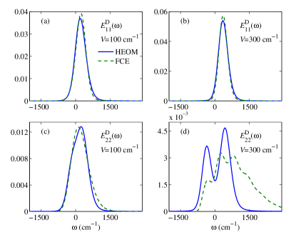
Figure 6: Comparison of the emission spectra obtained by the hierarchy equation of motion (HEOM) and the full 2nd-order cumulant expansion (FCE) methods. The reorganization energy is $\lambda=200\text{cm}^{-1}$.

The summation of $\alpha$ in Eq. (54) can be divided into two parts: (i) $\mu>\alpha$, and thus $\exp\left(\beta\omega_{\mu\alpha}\right)>1$. (ii) $\mu\leq\alpha$, and thus $\exp\left(\beta\omega_{\mu\alpha}\right)\leq 1$. If $|\mu\rangle$ is a low-excitated state, we have $\exp\left(\beta\omega_{\mu\alpha}\right)\leq 1$ for most $\alpha$, and $K_{\mu\mu}^{RI}$ will not become a very large value. On the opposite side, if $|\mu\rangle$ is a high-excitated state, $\omega_{\mu\alpha}$ could be a very large positive value and $\exp\left(\beta\omega_{\mu\alpha}\right)\gg 1$. In this case the matrix element $K_{\mu\mu}^{RI}$ could result in an unreliable dynamics of $E_{\mu\mu}^{D}\left(t\right)$.

Consider the Hamiltonian (53), we can obtain

$$K_{11}^{RI} \simeq i\frac{2\lambda e^{-\gamma t}}{\beta}\left(\frac{1}{\lambda^{2}}+\frac{e^{-2iVt}}{\lambda^{2}+\omega_{\mu\alpha}^{2}}e^{-2\beta V}\right),$$

$$K_{22}^{RI} \simeq i\frac{2\lambda e^{-\gamma t}}{\beta}\left(\frac{1}{\lambda^{2}}+\frac{e^{2iVt}}{\lambda^{2}+\omega_{\mu\alpha}^{2}}e^{2\beta V}\right),$$ (55)

where $K_{22}^{RI}$ contains a term that diverges as $\exp\left(2\beta V\right)$. In the energy representation, since all the matrices $\mathbf{K}^{II}$, $\mathbf{K}^{RR}$ and $\mathbf{K}^{RI}$ are diagonal, the emission spectrum matrix $\mathbf{E}^{D}\left(\omega\right)=\sum_{\mu}E_{\mu\mu}^{D}\left(\omega\right)|\mu\rangle\langle\mu|$ is also diagonal. In Fig. 6, we show the deviation of the emission spectra $E_{\mu\mu}^{D}\left(\omega\right)$ obtained by the cumulant expansion and the HEOM for different off-diagonal coupling $V$. The upper two panels show the emission spectrum of the lower excitation level $\mu=1$, for which the precision of the spectrum obtained by the cumulant expansion method is very reliable for different off-diagonal coupling $V$. However, from the lower panels of Fig. 6, the spectrum $E_{22}^{D}\left(\omega\right)$ obtained from the cumulant expansion deviates from the exact one as the increase of $V$.

Therefore, if the emission spectrum is determined mainly by the excited states that below the thermal energy, the cumulant expansion method is still reliable. This is the case when we calculate some far-field emission spectra, where the system’s dipole operators will select the lowest excited state.

IV.6 Multichromophoric FRET Rate

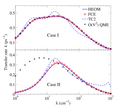
Figure 7: Comparison of multichromophoric FRET rates obtained by hierarchy equation of motion (HEOM), full 2nd-order cumulant expansion (FCE), TC2 Jang et al. (2004) and $O\left(V^{2}\right)$ quantum master equation (QME) methods, as a function of reorganization energy $\lambda$ for localized (25) and delocalized (26) cases. The bath parameters are the same as in Fig. 1.

After the study of spectra, we can calculate the multichromophoric FRET rate. In Fig. 7, we compare the multichromophoric FRET rate obtained via different methods. The exact results are obtained by HEOM. In this paper, the cumulant expansion is performed with respect to $\lambda$. We can also do perturbation with respect to the inter-site coupling $V$ of Eq.(3). This approach Cleary and Cao (2013) has a precision of $O\left(V^{2}\right)$, as shown in Fig. 7. For a localized system, $V$ is a good perturbative parameter, while for a delocalized system this method can give reliable results only for $\lambda\gg V$. The rate given by the TC2 method is qualitatively tolerant. It is not stable for very large reorganization energy.

Although the emission spectra could be not very precise for delocalized systems, the rate obtained by our cumulant expansion method is still in very good agreement with the exact one, since the multichromophoric FRET rate is proportional to the overlap integral between emission and absorption spectra. If the reorganization energy $\lambda$ is very large, the height of the spectra is very low and the overlap of the spectra is small.

V Conclusion

In this paper, we study the multichromophoric FRET rate and the spectra, based on a full 2nd-order cumulant expansion in both real- and imaginary-time domains, which treats the entire system-bath interaction Hamiltonian perturbatively, and can reduce to the exact FRET for monomers.

(i) In the emission spectrum, the initial state is an equilibrium state of the donor and its bath. Due to their interaction, both the donor and the bath deviate from their Boltzmann distributions. Moreover, the equilibrium state cannot be written in a factorized form, and the entanglement between the donor and its bath will affect the subsequent real-time dynamics. The failure of factorization approaches shows the crucial role of the donor-bath entanglement in both the emission spectrum and the multichromophoric FRET rate.

(ii) The FCE method is applied in both localized and delocalized systems. The absorption spectra obtained by the FCE method are in very good agreement with the exact results for both localized and delocalized cases. Further approximations of the FCE can give the IPR and the OCE methods, which overlook the importance of the off-diagonal system-bath coupling and fail to give reliable absorption spectra when the system is highly delocalized.

(iii) The calculation of the emission spectrum is more complicated due to the initial donor-bath entanglement, which depends on the donor-bath interaction and the degree of delocalization. For localized system, the entanglement is weak, and FCE method performs well. For delocalized system, the FCE method can still give reliable results for low-excitation state, while the method becomes unreliable for high-excitation states in the strong system-bath coupling regime. This problem is partially solved in our Paper II by combining the cumulant expansion with imaginary-time path integrals.

(iv) In contrast with the spectra, the multichromophoric FRET rate is more robust since it is proportional to the integral overlap between the emission and absorption spectra. The deviations in spectra are reduced in the transfer rate. Moreover, if the reorganization energy $\lambda$ is very large, the height of the spectra is very low and the overlap of the spectra is small. Thus, although the emission spectrum obtained by cumulant expansion could be not very reliable in strong system-bath coupling regime, we can still obtain a good enough transfer rate.

(v) The FCE method cannot give reliable emission spectra of delocalized systems, when the reorganization energy is large and the thermal energy is small. We develop several new methods to overcome this problem. When the reorganization energy $\lambda$ is dominate, perturbation can be carried out for system’s off-diagonal coupling $V$ up to its 2nd-order Cleary and Cao (2013). For more complicated systems such as the LH2, traditional perturbation methods fail to give reliable emission spectrum and multichromophoric FRET rate, since the energy gap of the first excitations, the thermal energy, and the reorganization energy are comparable. In our new developed hybrid cumulant expansion method, we use the imaginary-time path integrals to obtain the exact reduced density matrix of the donor, from which the displacements of the bath operators can be extracted more precisely. This hybrid method can give much more reliable emission spectrum and multichromophoric FRET rate for systems like LH2. Furthermore, to overcome the problems of the HEOM method in calculating large system and low-temperature conditions, we implement a complex-time stochastic path integrals method Moix et al. (2013), which gives us the benchmark.

Appendix A Bath correlation function and Lineshape matrices

A.1 Bath correlation function

The general form of the bath correlation function can be derived as

$$C^{B}\!\left(t\!-\!i\tau\right) \!\!\!= \!\!\!\int_{0}^{\infty}\frac{d\omega}{\pi}J\left(\omega\right)\frac{\cosh\left[\omega\left(\frac{1}{2}\beta-i\left(t-i\tau\right)\right)\right]}{\sinh\left[\frac{1}{2}\omega\beta\right]}$$ (56)

$$\!\!\!=\!\!\! \frac{4\lambda}{\beta}\bigg{\{}\frac{1}{2}e^{-\gamma\left|t\right|}\!\!+\!\!\gamma\sum_{k=1}^{\infty}\frac{\cos\left(\nu_{k}\tau\right)\left(\gamma e^{-\gamma\left|t\right|}\!\!-\!\!\nu_{k}e^{-\nu_{k}\left|t\right|}\right)}{\gamma^{2}-\nu_{k}^{2}}\!\!-\!\!i\text{sgn}\left(t\right)\gamma\sum_{k=1}^{\infty}\frac{\sin\left(\nu_{k}\tau\right)\left(\nu_{k}e^{-\gamma\left|t\right|}\!\!-\!\!\nu_{k}e^{-\nu_{k}\left|t\right|}\right)}{\gamma^{2}-\nu_{k}^{2}}\bigg{\}},$$

where $J\left(\omega\right)$ is the Drude spectrum, $\nu_{k}=2\pi k/\beta$ is the Matsubara frequency, and $\text{sgn}\left(x\right)$ is the sign function.

A.2 Lineshape matrix $\mathbf{K}\left(t\right)$

The matrix $\mathbf{K}\left(t\right)$ in Eq. (36) is given by

$$\mathbf{K}\left(t\right) = \!\int_{0}^{t}\!\!dt_{2}\int_{0}^{t_{2}}\!\!\!dt_{1}\text{tr}_{b}\left[H_{sb}^{A}\left(t_{2}\right)H_{sb}^{A}\left(t_{1}\right)\rho_{b}^{A}\right]$$ (57)

$$= \sum_{\mu,\nu=1}^{N_{A}}|\mu\rangle\langle\nu|\sum_{\alpha=1}^{N_{A}}\sum_{n=1}^{N_{A}}X_{n}^{\mu\alpha}X_{n}^{\alpha\nu}\!\int_{0}^{t}\!\!dt_{2}\int_{0}^{t_{2}}\!\!\!dt_{1}e^{i\omega_{\mu\alpha}t_{2}-i\omega_{\nu\alpha}t_{1}}C^{B}\left(t_{2}\!-t_{1}\!\right),$$

where the bath correlation function is

$$C^{B}\left(t_{2}-t_{1}\right) = \lambda\gamma\left[\cot\left(\frac{\gamma\beta}{2}\right)-i\right]e^{-\gamma\left|t_{2}-t_{1}\right|}+\frac{4\lambda\gamma}{\beta}\sum_{n=1}^{\infty}\frac{\nu_{n}e^{-\nu_{n}\left|t_{2}-t_{1}\right|}}{\nu_{n}^{2}-\gamma^{2}},$$

In the high-temperature limit we can neglect all the Matsubara terms, and thus

$$C^{B}\left(t_{2}-t_{1}\right)=\lambda\gamma\left[\cot\left(\frac{\gamma\beta}{2}\right)-i\right]e^{-\gamma\left|t_{2}-t_{1}\right|}.$$ (58)

In this case, the matrix elements can be derived as

$$K_{\mu\nu}\left(t\right) = \sum_{\alpha}\sum_{n}X_{n}^{\mu\alpha}X_{n}^{\alpha\nu}\int_{0}^{t}dt_{2}\int_{0}^{t_{2}}dt_{1}e^{i\omega_{\mu\alpha}t_{2}-i\omega_{\nu\alpha}t_{1}}C\left(t_{2}-t_{1}\right)$$

$$= \sum_{\alpha}\sum_{n}X_{n}^{\mu\alpha}X_{n}^{\alpha\nu}\lambda_{n}\gamma\left[\cot\left(\frac{\gamma\beta}{2}\right)-i\right]F_{\mu\alpha\nu}\left(t\right),$$

where

$$F_{\mu\alpha\nu}\left(t\right)=\frac{e^{-\gamma t+i\omega_{\mu\alpha}t}-1}{\left(\gamma-i\omega_{\mu\alpha}\right)\left(\gamma-i\omega_{\nu\alpha}\right)}+\frac{e^{i\omega_{\mu\nu}t}-1}{i\omega_{\mu\nu}\left(\gamma-i\omega_{\nu\alpha}\right)}.$$ (59)

If $\mu=\nu$, we have

$$F_{\mu\mu\mu} = \frac{e^{-\gamma t}-1}{\gamma^{2}}+\frac{t}{\gamma}.$$ (60)

A.3 Lineshape matrix $\mathbf{K}^{II}\left(\beta\right)$

The matrix $\mathbf{K}^{II}\left(\beta\right)$ in Eq. (46) is

$$\mathbf{K}^{II}\left(\beta\right) = \int_{0}^{\beta}\!\!d\tau_{2}\int_{0}^{\tau_{2}}\!\!\!d\tau_{1}\text{tr}_{b}\left[H_{sb}^{D}\!\!\left(-i\tau_{2}\right)H_{sb}^{D}\!\!\left(-i\tau_{1}\right)\rho_{b}^{D}\right]$$

$$= \sum_{\mu\nu\alpha}\sum_{n}X_{n}^{\mu\alpha}X_{n}^{\alpha\nu}|\mu\rangle\langle\nu|\int_{0}^{\beta}d\tau^{\prime}e^{\omega_{\mu\nu}\tau^{\prime}}\int_{0}^{\tau^{\prime}}d\tau\,e^{\omega_{\nu\alpha}\tau}C^{B}\left(-i\tau\right)$$

where the imaginary-time correlation function is

$$C^{B}\left(-i\tau\right) = \frac{2\lambda}{\beta}+\frac{4}{\beta}\sum_{k=1}^{\infty}\frac{\lambda\gamma}{\gamma+\nu_{k}}\cos\left(\nu_{k}\tau\right).$$ (61)

Substituting the above result into $\mathbf{K}^{II}$, we can solve the integral

$$\int_{0}^{\tau^{\prime}}d\tau\,e^{\omega_{\nu\alpha}\tau}C^{B}\left(-i\tau\right)=\frac{2\lambda}{\beta}\mathcal{F}_{\nu\alpha},$$ (62)

where

$$\mathcal{F}_{\nu\nu} = \tau^{\prime}+2\gamma\sum_{k=1}^{\infty}\frac{1}{\gamma+\nu_{k}}\frac{\sin\left(\nu_{k}\tau^{\prime}\right)}{\nu_{k}},$$

$$\mathcal{F}_{\nu\alpha} = \frac{e^{\omega_{\nu\alpha}\tau^{\prime}}-1}{\omega_{\nu\alpha}}+2\gamma\sum_{k=1}^{\infty}\frac{e^{\omega_{\nu\alpha}\tau^{\prime}}\left[\nu_{k}\sin\left(\nu_{k}\tau^{\prime}\right)+\omega_{\nu\alpha}\cos\left(\nu_{k}\tau^{\prime}\right)\right]-\omega_{\nu\alpha}}{\left(\gamma+\nu_{k}\right)\left(\nu_{k}^{2}+\omega_{\nu\alpha}^{2}\right)}.$$ (63)

A.4 Lineshape matrix $\mathbf{K}^{RR}\left(t,\beta\right)$

The matrix $\mathbf{K}^{RR}\left(t,\beta\right)$ in Eq. (48) is

$$\mathbf{K}^{RR}\left(t,\beta\right) = \!\!\int_{0}^{t}\!\!\!ds_{2}\int_{0}^{s_{2}}\!\!\!ds_{1}\text{tr}_{b}\left[H_{sb}^{D}\!\!\left(s_{2}\!\!-\!\!i\beta\right)H_{sb}^{D}\!\!\left(s_{1}\!\!-\!\!i\beta\right)\rho_{b}^{D}\right]$$

$$= \sum_{\mu\nu\alpha}\sum_{n}X_{n}^{\mu\alpha}X_{n}^{\alpha\nu}|\mu\rangle\langle\nu|e^{\beta\omega_{\mu\nu}}\int_{0}^{t}\!\!\!ds_{2}\,e^{i\omega_{\mu\nu}s_{2}}\int_{0}^{s_{2}}\!\!\!\!ds_{1}\,e^{i\omega_{\nu\alpha}s_{1}}\,C^{B}\left(s_{1}\right),$$

where

$$C^{B}\left(s\right) \simeq \lambda\gamma\left[\cot\left(\frac{\gamma\beta}{2}\right)-i\right]e^{-\gamma s}.$$ (64)

A.5 Lineshape matrix $\mathbf{K}^{RI}\left(t,\beta\right)$

The matrix $\mathbf{K}^{RI}\left(t,\beta\right)$ in Eq. (49) is

$$\mathbf{K}^{RI}\left(t,\beta\right) = \!\!\int_{0}^{t}\!\!\!ds\int_{0}^{\beta}\!\!\!d\tau\text{tr}_{b}\left[H_{sb}^{D}\!\!\left(s\!-\!i\beta\right)H_{sb}^{D}\!\!\left(-i\tau\right)\rho_{b}^{D}\right]$$

$$= \sum_{\mu\nu\alpha}\sum_{n}X_{n}^{\mu\alpha}X_{n}^{\alpha\nu}|\mu\rangle\langle\nu|e^{\beta\omega_{\mu\alpha}}\int_{0}^{t}\!\!\!ds\int_{0}^{\beta}\!\!\!\,d\tau e^{i\omega_{\mu\alpha}s-\omega_{\nu\alpha}\tau}C^{B}\!\left(-s\!-\!i\tau\right),$$

where

$$C^{B}\!\left(-s\!-\!i\tau\right) = \!\!\!\frac{4\lambda}{\beta}\bigg{\{}\frac{1}{2}e^{-\gamma s}+\gamma\sum_{k=1}^{\infty}\frac{\cos\left(\nu_{k}\tau\right)\left(\gamma e^{-\gamma s}-\nu_{k}e^{-\nu_{k}\tau}\right)}{\gamma^{2}-\nu_{k}^{2}}$$ (65)

$$+i\gamma\sum_{k=1}^{\infty}\frac{\sin\left(\nu_{k}\tau\right)\left(\nu_{k}e^{-\gamma s}-\nu_{k}e^{-\nu_{k}s}\right)}{\gamma^{2}-\nu_{k}^{2}}\bigg{\}}.$$

References

- Agranovich and Galanin (1982) V. M. Agranovich and M. D. Galanin, Electronic Excitation Energy Transfer in Condensed Matter, 3rd ed. (North-Holland Publishing Company, Amsterdam, 1982).
- Andrews and Demidov (1999) D. L. Andrews and A. A. Demidov, Resonance Energy Transfer (John Wiley and Sons, Chichester, 1999).
- May and Kühn (2004) V. May and O. Kühn, Charge and Energy Transfer Dy- namics in Molecular Systems (Wiley-VCH, Weinheim, 2004).
- Micha and Burghardt (2007) D. A. Micha and I. Burghardt, Quantum Dynamics of Complex Molecular Systems (Springer-Verlag Berlin Heidelberg, 2007).
- Förster (1965) T. Förster, Modern Quantum Chemistry, edited by O. Sinanoglu, Vol. 3 (Academic Press, New York, 1965).
- Blankenship (2002) R. E. Blankenship, Molecular Mechanisms of Photosynthesis (Blackwell Science, London, 2002).
- Renger et al. (2001) T. Renger, V. May, and O. Kühn, Phys. Rep., 343, 137 (2001).
- Novoderezhkin and Grondelle (2010) V. I. Novoderezhkin and R. v. Grondelle, PCCP, 12, 7352 (2010).
- Varnavski et al. (2002) O. Varnavski, I. D. W. Samuel, L.-O. Pålsson, R. Beavington, P. L. Burn, and T. Goodson, J. Chem. Phys., 116, 8893 (2002).
- Nguyen et al. (2000) T.-Q. Nguyen, J. Wu, V. Doan, B. J. Schwartz, and S. H. Tolbert, Science, 288, 652 (2000).
- Bopp et al. (1999) M. A. Bopp, A. Sytnik, T. D. Howard, R. J. Cogdell, and R. M. Hochstrasser, Proc. Natl. Acad. Sci. USA, 96, 11271 (1999).
- Oijen et al. (1999) A. M. v. Oijen, M. Ketelaars, J. Köhler, T. J. Aartsma, and J. Schmidt, Science, 285, 400 (1999).
- Ye et al. (2012) J. Ye, K. Sun, Y. Zhao, Y. Yu, C. Kong Lee, and J. Cao, J. Chem. Phys., 136, 245104 (2012).
- Collini et al. (2010) E. Collini, C. Y. Wong, K. E. Wilk, P. M. G. Curmi, P. Brumer, and G. D. Scholes, Nature, 463, 644 (2010).
- Engel et al. (2007) G. S. Engel, T. R. Calhoun, E. L. Read, T.-K. Ahn, T. Mančal, Y.-C. Cheng, R. E. Blankenship, and G. R. Fleming, Nature, 446, 782 (2007).
- Mercer et al. (2009) I. P. Mercer, Y. C. El-Taha, N. Kajumba, J. P. Marangos, J. W. G. Tisch, M. Gabrielsen, R. J. Cogdell, E. Springate, and E. Turcu, Phys. Rev. Lett., 102, 057402 (2009).
- Lee et al. (2007) H. Lee, Y.-C. Cheng, and G. R. Fleming, Science, 316, 1462 (2007).
- Ishizaki et al. (2010) A. Ishizaki, T. R. Calhoun, G. S. Schlau-Cohen, and G. R. Fleming, PCCP, 12, 7319 (2010).
- Abramavicius et al. (2009) D. Abramavicius, B. Palmieri, D. V. Voronine, F. Šanda, and S. Mukamel, Chem. Rev., 109, 2350 (2009).
- Cho (2008) M. Cho, Chem. Rev., 108, 1331 (2008).
- Jonas (2003) D. M. Jonas, Science, 300, 1515 (2003).
- Herek et al. (2000) J. L. Herek, N. J. Fraser, T. Pullerits, P. Martinsson, T. Polivka, H. Scheer, R. J. Cogdell, and V. Sundstrom, Biophys. J., 78, 2590 (2000).
- Hu et al. (2002) X. Hu, T. Ritz, A. Damjanovic, F. Autenrieth, and K. Schulten, Q. Rev. Biophys., 35, 1 (2002).
- Beljonne et al. (2009) D. Beljonne, C. Curutchet, G. D. Scholes, and R. J. Silbey, J. Phys. Chem. B, 113, 6583 (2009).
- Sumi (1999) H. Sumi, J. Phys. Chem. B, 103, 252 (1999).
- Scholes (2003) G. D. Scholes, Annu. Rev. Phys. Chem., 54, 57 (2003).
- Jang et al. (2004) S. Jang, M. D. Newton, and R. J. Silbey, Phys. Rev. Lett., 92, 218301 (2004).
- Wu and Cao (2013) J. Wu and J. Cao, J. Chem. Phys., 139, 044102 (2013).
- Mennucci and Curutchet (2011) B. Mennucci and C. Curutchet, PCCP, 13, 11538 (2011).
- Mukamel (1995) S. Mukamel, Principles of Nonlinear Optical Spectroscopy (Oxford University Press, 1995).
- Moix et al. (2013) J. Moix, J. Ma, and J. Cao, prepare (2013).
- Tanimura (2006) Y. Tanimura, J. Phys. Soc. Jpn., 75, 082001 (2006).
- Tanimura (1993) Y. Tanimura, Phys. Rev. E, 47, 118 (1993).
- Ishizaki and Fleming (2009) A. Ishizaki and G. R. Fleming, PNAS, 106, 17255 (2009a).
- Ishizaki and Fleming (2009) A. Ishizaki and G. R. Fleming, J. Chem. Phys., 130, 234111 (2009b).
- Chen et al. (2009) L. Chen, R. Zheng, Q. Shi, and Y. Yan, J. Chem. Phys., 131, 094502 (2009).
- Strümpfer and Schulten (2011) J. Strümpfer and K. Schulten, J. Chem. Phys., 134, 095102 (2011).
- Jing et al. (2013) Y. Jing, L. Chen, S. Bai, and Q. Shi, J. Chem. Phys., 138, 045101 (2013).
- Jang and Silbey (2003) S. Jang and R. J. Silbey, J. Chem. Phys., 118, 9324 (2003).
- Renger and Marcus (2002) T. Renger and R. A. Marcus, J. Chem. Phys., 116, 9997 (2002).
- Banchi et al. (2013) L. Banchi, G. Costagliola, A. Ishizaki, and P. Giorda, J. Chem. Phys., 138, 184107 (2013).
- Maier et al. (2011) S. Maier, T. L. Schmidt, and A. Komnik, Phys. Rev. B, 83, 085401 (2011).
- Lee et al. (2012) C. K. Lee, J. Moix, and J. Cao, J. Chem. Phys., 136, 204120 (2012).
- Yang (2005) M. Yang, J. Chem. Phys., 123, 124705 (2005).
- Zhang et al. (1998) W. M. Zhang, T. Meier, V. Chernyak, and S. Mukamel, J. Chem. Phys., 108, 7763 (1998).
- Kolli et al. (2011) A. Kolli, A. Nazir, and A. Olaya-Castro, J. Chem. Phys., 135, 154112 (2011).
- Novoderezhkin et al. (2004) V. I. Novoderezhkin, M. A. Palacios, H. van Amerongen, and R. van Grondelle, J. Phys. Chem. B, 108, 10363 (2004).
- Cho et al. (2005) M. Cho, H. M. Vaswani, T. Brixner, J. Stenger, and G. R. Fleming, J. Phys. Chem. B, 109, 10542 (2005).
- Yang and Fleming (2002) M. Yang and G. R. Fleming, Chem. Phys., 282, 163 (2002).
- Ohta et al. (2001) K. Ohta, M. Yang, and G. R. Fleming, J. Chem. Phys., 115, 7609 (2001).
- Schröder et al. (2006) M. Schröder, U. Kleinekathöfer, and M. Schreiber, J. Chem. Phys., 124, 084903 (2006).
- Yang et al. (2004) S. Yang, J. Shao, and J. Cao, J. Chem. Phys., 121, 11250 (2004).
- Cleary and Cao (2013) L. Cleary and J. Cao, New J. Phys. to appear (2013a).
- Ma et al. (2013) J. Ma, J. Moix, and J. Cao, prepare (2013).
- Cleary and Cao (2013) L. Cleary and J. Cao, prepare (2013b).
- Wu et al. (2010) J. Wu, F. Liu, Y. Shen, and J. Cao, New J. Phys., 12, 105012 (2010).
- Moix et al. (2012) J. Moix, Y. Zhao, and J. Cao, Phys. Rev. B, 85, 115412 (2012).
- Cleary et al. (2013) L. Cleary, H. Chen, C. Chuang, R. J. Silbey, and J. Cao, Proc. Natl. Acad. Sci. USA, 110, 8537 (2013).