Analysing kinetic transition networks for rare events

Abstract

The graph transformation approach is a recently proposed method for computing mean first passage times, rates, and committor probabilities for kinetic transition networks. Here we compare the performance to existing linear algebra methods, focusing on large, sparse networks. We show that graph transformation provides a much more robust framework, succeeding when numerical precision issues cause the other methods to fail completely. These are precisely the situations that correspond to rare event dynamics for which the graph transformation was introduced.

The kinetics of many complex physical processes can be described by kinetic transition networks NoeF08 ; pradag09 . In these networks the discrete states correspond to the nodes of a graph, whose edges encode the underlying transitions. In many situations the Markov approximation holds and transitions between the states are taken to be independent random processes. These kinetic transition networks can also be viewed as continuous time Markov processes. They are widely used in the physical sciences, and also in other fields such as finance masoliver.2006 and modelling of social networks acemoglu.2013 . In protein folding studies the states and rates are often defined by data gathered from molecular dynamics simulations NoeSVRW09 . Alternatively, the states may be local minima on the potential energy landscape, where the rate constants are calculated from unimolecular rate theory wales02 ; wales04 .

Rate constants are local properties specifying the time scale on which direct transitions between states occur. However, we usually want to calculate experimental observables, such as the mean first passage time (MFPT) between two states. These global properties of the network can be computed stochastically, e.g. using kinetic Monte Carlo simulations HenkelmanJ01 , or, if the number of states is small enough, by directly solving the master equation through matrix diagonalization. Unfortunately, stochastic methods are approximate and can be rather slow to converge, while the exact methods tend to suffer from numerical precision problems glowacki.2012 due to poorly conditioned matrices. This situation is likely to be encountered for rare events, where the range of relaxation times can span many orders of magnitude. Here we discuss the performance of a recently introduced method for computing global kinetic quantities called the new graph transformation (NGT) approach Wales09 and compare it to existing methods. We show how NGT overcomes the numerical precision problems that plague other methods with little additional overhead in terms of computing time.

Consider a kinetic transition network NoeF08 ; pradag09 ; Wales10a with $N$ nodes and $E$ edges. To each edge $u\to v$ is associated a rate constant $k_{uv}$. It is convenient to define the rate matrix $R_{uv}$ as

$$R_{uv}=k_{uv}\text{ \quad for }u\neq v\quad{\rm with}\quad\sum_{v}R_{uv}=0.$$ (1)

The second condition specifies that the diagonal components are given by $R_{uu}=-\sum_{v}k_{uv}$. The kinetic transition network can be equivalently expressed in terms of transition probabilities $P_{uv}$ and waiting times $\tau_{u}$, where

$$\tau_{u}=\left(\sum_{v}k_{uv}\right)^{-1}\text{ \quad and \quad}P_{uv}=\tau_{u}k_{uv}.$$ (2)

We further specify a product group $A$ and a reactant group $B$, which may consist of multiple nodes, for which we want to compute rates and MFPTs.

We can specify the MFPT $T_{uB}$, the mean time for a trajectory starting at $u$ to reach a node in $B$, in terms of the MFPTs of the neighbours of $u$ as $T_{uB}=\tau_{u}+\sum_{x}P_{ux}T_{xB}$. Written in terms of $R$ this becomes norris.1997

$$\sum_{x\notin B}R_{ux}T_{xB}=-1\text{\quad\quad for }u\notin B.$$ (3)

This is a system of linear equations, which can be solved for the vector $\{T_{uB}|u\notin B\}$. If the product group $A$ contains more than one node, the transition rate from $A$ to $B$ is an average over the inverse MFPT for each element $a$ in $A$, weighted by their equilibrium occupation probability, $p^{\text{eq}}_{a}$

$$k_{AB}=\left<\frac{1}{T_{aB}}\right>_{a\in A}=\frac{1}{\sum_{a\in A}p^{\text{eq}}_{a}}\sum_{a\in A}\frac{p^{\text{eq}}_{a}}{T_{aB}}.$$ (4)

Committor probabilities, the probability that node $u$ will reach $B$ before it reaches $A$, are defined such that $q_{u}=0$ if $u\in A$, and $q_{u}=1$ if $u\in B$. For $u\notin A\cup B$ they can be found via the relation $q_{u}=\sum_{v}P_{uv}q_{v}$. In terms of R, this becomes

$$\sum_{x\notin A\cup B}R_{ux}q_{x}=-\sum_{b\in B}R_{ub}\text{ \quad for }u\notin A\cup B.$$ (5)

which can be solved numerically for the vector $\{q_{u}|u\notin A\cup B\}$ norris.1997 ; metznersv09 .

The NGT method is a deterministic graph renormalization procedure Wales09 ; trygubenkoW06a ; trygubenkow06b to compute the exact MFPT averaged over the product group $B$, for any member of the reactant group $A$. We use ‘renormalization’ in the sense of real space renormalization group theory landau.2005 . Nodes are deterministically removed and the waiting times and branching probabilities of neighbouring nodes are updated so that the MFPT for any reactant state averaged over all the product states is preserved; the proof does not require detailed balance Wales09 ; trygubenkoW06a ; trygubenkow06b . Each node $u$ is also assigned a loop edge $u\to u$ pointing back to itself. In the typical case, the self-transition probabilities $P_{uu}$ will all be zero initially, but will take non-zero values after renormalization. The transition probabilities always satisfy $\sum_{v}P_{uv}=1$.

Upon removing node $x$, the updated transition probabilities are found by summing the direct path from $u$ to $v$ and all paths through $x$

$$P_{uv}\to P_{uv}+P_{ux}P_{xv}\sum_{m=0}^{\infty}P_{xx}^{m}$$

$$\to P_{uv}+\frac{P_{ux}P_{xv}}{1-P_{xx}}.$$ (6)

The self-transition probabilities $P_{uu}$ are updated according to the same equation. Similarly, the updated waiting time $\tau_{u}$ is found by computing the mean time to reach one of the neighbours of $u$ (excluding $x$), or to return to $u$.

$$\tau_{u}\to \sum_{v\neq x}\left\{P_{uv}\tau_{u}+P_{ux}P_{xv}\sum_{m=0}^{\infty}\left[\tau_{u}+(m+1)\tau_{x}\right]P_{xx}^{m}\right\}$$

$$\to \tau_{u}+\frac{P_{ux}\tau_{x}}{1-P_{xx}}.$$ (7)

Equations 6 and 7 constitute the NGT graph renormalization procedure.

We wish to compute the mean first passage time from node $a\in A$ to the product group of nodes $B$. Nodes are iteratively removed from the graph, updating the graph attributes according to 6 and 7), until the only remaining nodes are $a$ and $b\in B$. In this reduced graph, every trajectory starting from $a$ (except those following the loop edge $a\to a$) will transition directly to $B$. The MFPT is, then, found from the relation $T_{aB}=\tau_{a}+P_{aa}T_{aB}$, which leads directly to

$$T_{aB}=\frac{\tau_{a}}{1-P_{aa}}.$$ (8)

The rate from $A$ to $B$ can then be computed via equation 4. The calculation, in practice, is performed in two phases. First, the intervening nodes (not in $A$ or in $B$) are all removed from the graph. Then for each node $a\in A$ we compute $T_{aB}$ by removing from the graph all nodes in $A$ except $a$. The rates $B\to A$ can be computed in a similar manner.

Solving for the committor probability is straightforward in the NGT framework. Using equations 6 and 7 we first remove all nodes in the graph except those in $A$, $B$, and $u$ itself. We can then read off the committor probability as Wales09

$$q_{u}=\frac{\sum_{b\in B}P_{ub}}{\sum_{x\in A\cup B}P_{ux}}\text{ \quad for }u\notin A\cup B.$$ (9)

The denominator can also be written as $1-P_{uu}$. In reference Wales09 the committor is defined as $C_{u}^{B}$ in a slightly different way. For $u\notin A\cup B$ it is equivalent to $q_{u}$, but $C_{u}^{B}$ can take non-zero values for $u\in A$.

In equations 6, 7, and 8 we can compute $1-P_{uu}$ in two different ways via the relation

$$1-P_{uu}=\sum_{v\neq u}P_{uv}.$$ (10)

This procedure allows us to maintain numerical precision when $P_{uu}$ is very small and when $P_{uu}$ is very close to 1.

There are some important differences between NGT and the linear algebra method. Solving the system of linear equations results in the MFPT (or committor) for every node in the graph. In contrast, the MFPTs (and committors) for NGT are treated one node at a time. If we are interested in $k_{AB}$, and $A$ is not too large, the additional overhead is minor. On the other hand, when computing $k_{AB}$ with the NGT method, the reverse rate $k_{BA}$ is obtained essentially for free.

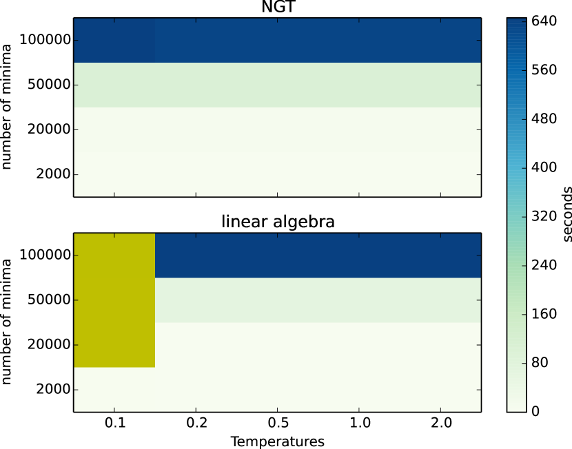
Figure 1: CPU time required to compute rates with NGT and a sparse linear algebra solver for the LJ₃₈ cluster as a function of temperature and the number of nodes. Yellow indicates that the method failed.

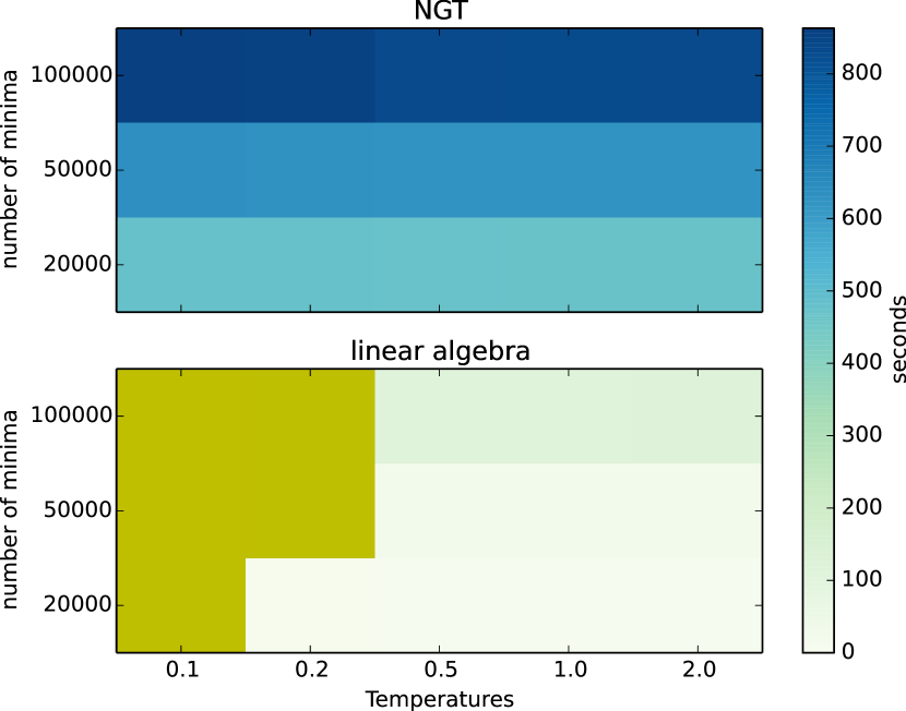
Figure 2: CPU time required to compute rates with NGT and a sparse linear algebra solver for the LJ₇₅ cluster as a function of temperature and the number of nodes. Yellow indicates that the method failed.

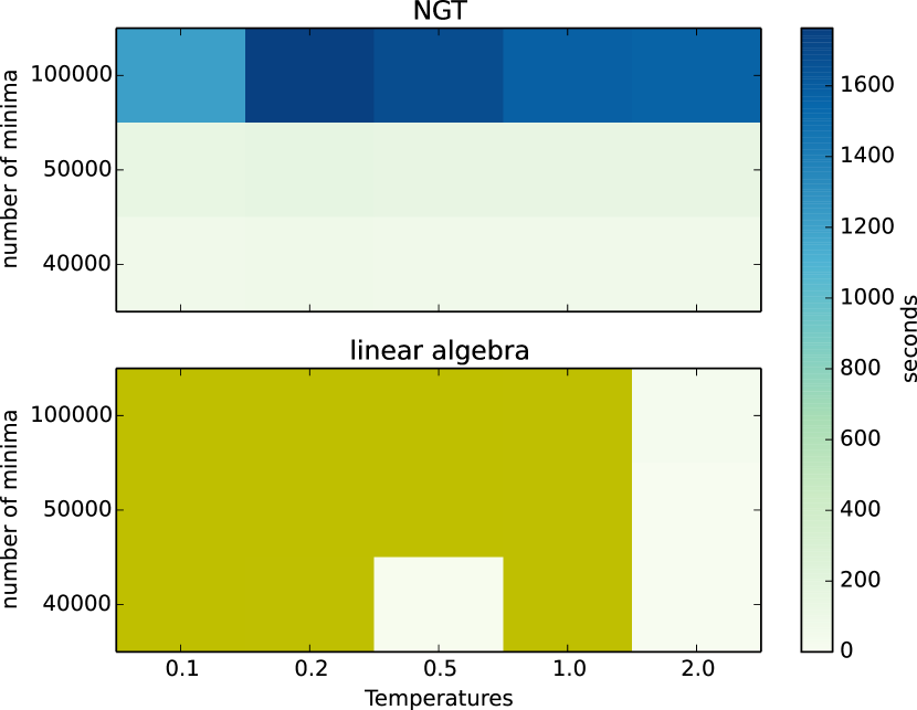
Figure 3: CPU time required to compute rates with NGT and a sparse linear algebra solver for the three-stranded $\beta$-sheet peptide Beta3s as a function of temperature and the number of nodes. Yellow indicates that the method failed.

To compare the performance of the NGT method with the linear algebra approach we chose several benchmark systems that are representative of important problems in rare event dynamics. We consider two Lennard-Jones clusters of 38 atoms doyemw99 and 75 atoms doyemw99 , denoted LJ₃₈ and LJ₇₅, along with the three-stranded $\beta$-sheet peptide Beta3s carrw08 . The networks were generated in previous discrete path sampling studies wales02 ; wales04 . The nodes of these networks represent minima on the potential energy landscape (locally stable configurations), while the edges correspond to transition states connecting the minima. These stationary points were computed numerically using geometry optimization techniques wales03 . The rate constants $k_{uv}$ were calculated according to transition state theory. All numerical computations were performed using our public domain software packages GMIN, OPTIM, and PATHSAMPLE.

The examples considered here correspond to relatively sparse networks of between 2000 and 100000 nodes. Typically the number of edges was several times the number of nodes. Hence we compared NGT with the C-language sparse linear algebra package UMFPACK umfpack , which employs sparse LU factorization. UMFPACK is contained in the python scientific computing package SciPy scipy . We tried several other methods for solving the linear equations, including SuperLU superlu , another sparse LU decomposition package; conjugate gradient iteration scipy ; and, after symmetrizing $R$, sparse Cholesky decomposition using CHOLMOD cholmod . All of these methods exhibited similar or poorer performance than UMFPACK.

We report here only the results for the MFPTs. Computing committors for NGT uses exactly the same procedure. Calculating committors with linear algebra requires solving a different system of linear equations, but the performance results are very similar to those for the mean first passage times.

The results for computing the MFPTs between two groups of nodes are shown in figures 1 and 2 for the LJ₃₈ and LJ₇₅ clusters, and figure 3 for the three-stranded $\beta$ sheet peptide. When the procedures agree, the sparse linear solver is about 1.5 times faster than NGT for LJ₃₈, and about an order of magnitude faster for LJ₇₅. However, the linear algebra approaches often fail, returning unphysical results, such as negative mean first passage times.

The linear algebra solvers fail more often for larger systems, and rarely work for the lower temperatures that are the main focus of interest for rare event dynamics. For low temperatures, the largest and smallest relaxation times can differ by many orders of magnitude. This ill-conditioning leads to the possibility of large errors arising from numerical imprecision.

The special property of the rate matrix $\sum_{v}R_{uv}=0$ means that precision issues are a problem from the beginning. This property is reflected in the transition probabilities, which conserve the total probability. The problem can be understood by the fact that a floating point number cannot precisely represent values arbitrarily close to zero or arbitrarily close to one. The NGT method was specifically designed to solve these problems. At every step in the graph renormalization, the transition probabilities at each node $u$ satisfy $\sum_{v}P_{uv}=1$. This condition means that when computing $1-P_{uu}$ we can either use $1-P_{uu}$ directly or indirectly via $\sum_{v\neq u}P_{uv}$. In practice we use the former definition unless $P_{uu}>0.99$. We believe this procedure accounts for the fact that the linear algebra method fails regularly, while NGT always produces a sensible result. It is possible that a preconditioning procedure could be derived that increases the stability of the linear algebra method, but we have not yet found a method that improves the present results.

In summary, we have compared the performance of the NGT algorithm for computing mean first passage times and committor probabilities with sparse linear algebra packages. We have shown that the linear algebra packages can be somewhat faster, but frequently fail at the lower temperatures of interest. We believe that this result is due to problems with numerical precision, which occur when the ratio of the largest relaxation time to the smallest is large. The NGT algorithm avoids these numerical problems by taking advantage of the physical structure of the problem to precisely represent important probabilities that are arbitrarily close to zero or unity.

Systems that exhibit multifunnel energy landscapes doyemw99 , with competing morphologies separated by high barriers, exhibit interesting properties. Low temperature heat capacity peaks correspond to broken ergodicity, and multiple relaxation time scales reflect rare event dynamics Wales10a . Such landscapes present significant challenges for global optimisation and sampling. Recent developments for analysing thermodynamics NeirottiCFD00 ; CalvoNFD00 ; MandelshtamFC06 ; SharapovMM07 ; SharapovM07 ; Calvo10 ; SehgalMF14 and kinetics PiccianiAKT11 will enable us to validate the approximations that make computational potential energy landscape approaches, such as basin-sampling BogdanWC06 ; Wales2013 and discrete path sampling wales02 ; wales04 ; Wales06 , so efficient. The present work provides another key piece of information, confirming the accuracy of the NGT procedure for extracting rates from kinetic transition networks, and the efficiency of the method for treating the dynamics of multi-funnel landscapes.

- (1) F. Noé and S. Fischer, Curr. Op. Struct. Biol. 18, 154 (2008).
- (2) D. Prada-Gracia, J. Gómez-Gardenes, P. Echenique, and F. Fernando, PLoS Comput. Biol. 5, 1 (2009).
- (3) J. Masoliver, M. Montero, J. Perello, and G. H. Weiss, J. Economic Behavior and Organization 61, 577 (2006).
- (4) D. Acemoglu, G. Como, F. Fagnani, and A. Ozdaglar, Math. Oper. Res. 38, 1 (2013).
- (5) F. Noe, C. Schutte, E. Vanden-Eijnden, L. Reich, and T. R. Weikl, Proc. Nat. Acad. Sci. USA 106, 19011 (2009).
- (6) D. J. Wales, Mol. Phys. 100, 3285 (2002).
- (7) D. J. Wales, Mol. Phys. 102, 891 (2004).
- (8) G. Henkelman and H. Jónsson, J. Chem. Phys. 115, 9657 (2001).
- (9) D. R. Glowacki, C.-H. Liang, C. Morley, M. J. Pilling, and S. H. Robertson, J. Phys. Chem. A 116, 9545 (2012).
- (10) D. J. Wales, J. Chem. Phys. 130, 204111 (2009).
- (11) D. J. Wales, Curr. Op. Struct. Biol. 20, 3 (2010).
- (12) J. R. Norris, Markov Chains, Cambridge University Press, 1997.
- (13) P. Metzner, C. Schütte, and E. Vanden-Eijnden, Multiscale Model. Simul. 7, 1192 (2009).
- (14) S. A. Trygubenko and D. J. Wales, Mol. Phys. 104, 1497 (2006).
- (15) S. A. Trygubenko and D. J. Wales, J. Chem. Phys. 124, 234110 (2006).
- (16) D. Landau and K. Binder, A Guide to Monte Carlo Simulations in Statistical Physics, Cambridge University Press, New York, NY, USA, 2005.
- (17) J. P. K. Doye, M. A. Miller, and D. J. Wales, J. Chem. Phys. 110, 6896 (1999).
- (18) J. M. Carr and D. J. Wales, J. Phys. Chem. B 112, 8760 (2008).
- (19) D. J. Wales, Energy Landscapes, Cambridge University Press, Cambridge, 2003.
- (20) T. A. Davis, ACM Trans. Math. Software 30, 196 (2004).
- (21) E. Jones et al., SciPy: Open source scientific tools for Python, 2001–.
- (22) X. S. Li, ACM Trans. Math. Software 31, 302 (2005).
- (23) Y. Chen, T. A. Davis, W. W. Hager, and S. Rajamanickam, ACM Trans. Math. Software 35 (2009).
- (24) J. P. Neirotti, F. Calvo, D. L. Freeman, and J. D. Doll, J. Chem. Phys. 112, 10340 (2000).
- (25) F. Calvo, J. P. Neirotti, D. L. Freeman, and J. D. Doll, J. Chem. Phys. 112, 10350 (2000).
- (26) V. A. Mandelshtam, P. A. Frantsuzov, and F. Calvo, J. Phys. Chem. A 110, 5326 (2006).
- (27) V. A. Sharapov, D. Meluzzi, and V. A. Mandelshtam, Phys. Rev. Lett. 98, 105701 (2007).
- (28) V. A. Sharapov and V. A. Mandelshtam, J. Phys. Chem. A 111, 10284 (2007).
- (29) F. Calvo, Phys. Rev. E 82, 046703 (2010).
- (30) R. M. Sehgal, D. Maroudas, and D. M. Ford, J. Chem. Phys. 140, (2014).
- (31) M. Picciani, M. Athenes, J. Kurchan, and J. Tailleur, J. Chem. Phys. 135, 034108 (2011).
- (32) T. V. Bogdan, D. J. Wales, and F. Calvo, J. Chem. Phys. 124, 044102 (2006).
- (33) D. J. Wales, Chem. Phys. Lett. 584, 1 (2013).
- (34) D. J. Wales, Int. Rev. Phys. Chem. 25, 237 (2006).