On Queue-Size Scaling for Input-Queued Switches

Abstract

We study the optimal scaling of the expected total queue size in an $n\times n$ input-queued switch, as a function of the number of ports $n$ and the load factor $\rho$, which has been conjectured to be $\Theta(n/{(}1-\rho{)})$ (cf. [13]). In a recent work [14], the validity of this conjecture has been established for the regime where $1-\rho=O(1/n^{2})$. In this paper, we make further progress in the direction of this conjecture. We provide a new class of scheduling policies under which the expected total queue size scales as $O\big{(}n^{1.5}(1-\rho)^{-1}\log\big{(}1/(1-\rho)\big{)}\big{)}$ when $1-\rho=O(1/n)$. This is an improvement over the state of the art; for example, for $\rho=1-1/n$ the best known bound was $O(n^{3})$, while ours is $O(n^{2.5}\log n)$.

D. Shahlabel=e1]devavrat@mit.edu J. N. Tsitsiklislabel=e1]jnt@mit.edu Y. Zhonglabel=e1]zhyu4118@mit.edu ds.ackMay 18, 2014. This work was supported by NSF grants CCF-0728554 and CMMI-1234062. This research was performed while all authors were affiliated with the Laboratory for Information and Decision Systems as well as the Operations Research Center at MIT. The third author is currently with the IEOR department, at Columbia University. Current emails: {devavrat,jnt}@mit.edu, yz2561@columbia.edu.

1 Introduction

An input-queued switch is a popular and commercially available architecture for scheduling data packets in an internet router. In general, an input-queued switch maintains a number of virtual queues to which packets arrive. Packets to be served at each time slot are selected according to a scheduling policy, subject to system constraints that specify which queues can be served simultaneously.

The input-queued switch model is an important example of so-called “stochastic processing networks,” formalized by Harrison [4, 5], which have become a canonical model of a variety of dynamic resource allocation scenarios. While the most basic questions concerning throughput and stability are relatively well-understood for general stochastic processing networks (see e.g., [9], [7], [6], [2], [16], [10], [17]), much less is known on the subject of more refined performance measures (e.g., results on the distribution and the moments of queue sizes), even for the special context of input-queued switches.

This paper contributes to the performance analysis of stochastic processing networks. It is motivated by the conjectures put forth in [13] on the optimal scaling of the expected total queue size in an $n\times n$ input-queued switch, as a function of the number of ports $n$ and the load factor $\rho$. For certain limiting regimes, it was conjectured in [13] that the optimal scaling (that is, the scaling under an “optimal” policy) takes the form $\Theta\left(n/(1-\rho)\right)$. This is to be compared to available results that include an ${O(}n^{2}/(1-\rho))$ upper bound, achieved by the so-called Maximum-Weight policy [12], [8], and an $O(n\log n/(1-\rho)^{2})$ upper bound, achieved by a batching policy proposed in [11]. More recently, Shah et al. [14] proposed a policy that gives an upper bound of $\frac{n}{1-\rho}+n^{3}$, thus establishing the validity of the conjecture when $1-\rho=O(1/n^{2})$.

In this paper, we focus on a different regime, where $1/n^{2}\ll 1-\rho\leq 1/n$. In some sense, this is a more difficult regime to analyze, when compared to the regime where $1-\rho=O(1/n^{2})$. This is because we consider a larger “gap” $1-\rho$, and so the heavy-traffic aspects of the system are less pronounced. This in turn means that various laws of large numbers (e.g., fluid or batching arguments) are less effective.

Concretely, we shall focus on the case $\rho=1-1/{f_{n}}$, where $f_{n}\geq n$ for all $n$, and for $n$ tending to infinity. When $f_{n}=n$, previous works give an upper bound $O(n^{3})$ (ignoring poly-logarithmic dependence on $n$) on the expected total queue size. In contrast, when $\rho=1-1/n$, the conjectured optimal scaling $O\left(n/(1-\rho)\right)$ is of the form $O(n^{2})$. It is then natural to ask whether this gap can be reduced, i.e., whether there exists a policy under which the expected total queue size is upper bounded by $O(n^{\alpha})$, with $\alpha<3$ (and ideally with $\alpha=2$), when $\rho=1-1/n$.

Our main contribution is a new policy that leads to an upper bound of $O\big{(}n^{1.5}f_{n}\log f_{n}\big{)}$, when $f_{n}\geq n$ and the arrival rates at the different queues are all equal. As a corollary, if $f_{n}=n$, the expected total queue size is upper bounded by $O(n^{2.5}\log n)$. This is the best known scaling with respect to $n$, when $\rho=1-1/n$. While this is a significant improvement over existing bounds, we still believe that the right scaling (ignoring any poly-logarithmic factors) is $O(n^{2})$. The best currently known scalings on the expected total queue size under various regimes, in an $n\times n$ input-queued switch, are summarized in Table 1.

Table 1: Best known scalings of the expected total queue size in various regimes. Here, $\rho$ is the load factor and $n$ is the number of input ports.

Regime	Scaling	References
$\frac{1}{1-\rho}<n$	$O\left(\frac{n\log n}{(1-\rho)^{2}}\right)$	[11]
$\frac{1}{1-\rho}=n$	$O\left(n^{2.5}\log n\right)$	this work
$n\leq\frac{1}{1-\rho}<n^{2}$	$O\left(\frac{n^{1.5}\log n}{1-\rho}\right)$	this work
$\frac{1}{1-\rho}\geq n^{2}$	$\Theta\left(\frac{n}{1-\rho}\right)$	[14]

The policy that we propose is a variation of the standard batching policy. In the standard batching policy, time is divided into disjoint intervals or batches. Packets that arrive in a given batch are served only after the arrival of the entire batch. By choosing the batch length large enough (deterministically or randomly), the total number of arriving packets is close to its expected value and can be served efficiently. In general, a longer batching interval improves efficiency, because the effect of random fluctuations is less pronounced, but on the other hand leads to larger delays and queue sizes. For this reason, a good batching policy, as for example in [11], selects the smallest possible batch length that will guarantee stability; in [11], this led to a bound of $O\left(\frac{n\log n}{(1-\rho)^{2}}\right)$ on the expected total queue size.

Given the stability requirement, we cannot hope to improve delay by reducing the batch length. On the other hand, the policy that we consider starts serving packets from a given batch a lot earlier, before the arrival of the entire batch. By starting to serve early, the expected delay (and hence queue size) is reduced. When the arrival rates at each queue are all equal, we show that the arrival process has sufficient regularity at a time scale shorter than the batch length. Consequently, the policy can indeed start serving the arriving packets early, while making sure that the stochastic fluctuations lead to only a small number of unserved packets, which can be “cleared” efficiently at the end of the batch. The combination of these ideas results in substantial improvement over the standard batching policy.

A few remarks are in order regarding the proposed policy. Our policy relies on the assumption of uniform arrival rates. In contrast, some existing policies, such as the maximum weight policy or the one in [14], are based only on the observed system state (the queue sizes) and are effective even with non-uniform arrival rates. However, we believe that our policy and its analysis can be modified to account for general (non-uniform) arrival rates.

1.1 Organization

The rest of the paper is organized as follows. In Section 2, we describe the input-queued switch model. In Section 3, we state our main theorem. In Section 4, we introduce some preliminary facts and theorems, which will be used in later sections. In Section 5, we describe our policy. In Section 6, we provide the proof of the main theorem. We conclude with some discussion in Section 7.

2 Input-queued switch model

An $n\times n$ input-queued switch has $n$ input ports and $n$ output ports. The switch operates in discrete time, indexed by $\tau\in{\{1,2,\dots\}}$. In each time slot, and for each port pair $(i,j)$, a unit-sized packet may arrive at input port $i$ destined for output port $j$, according to an exogenous arrival process. Let $A_{i,j}(\tau)$ denote the cumulative number of such arriving packets during time slots $1,\ldots,\tau$. We assume that the processes $A_{i,j}(\cdot)$ are independent for different pairs $(i,j)$. Furthermore, for every input-output pair $(i,j)$, $\{A_{i,j}(\tau)-A_{i,j}(\tau-1)\}_{\tau\in\mathbb{N}}$ is a Bernoulli process with parameter $\rho/n$, with the convention that $A_{i,j}(0)=0$. In particular,

$${\mathbb{E}[}A_{i,j}(\tau)]={{\frac{\rho}{n}\tau}},\quad{\mbox{for \ all\ }i,j,\ \mbox{and all }\tau\geq 1.}$$

We are only interested in systems that can be made stable under a suitable policy, and for this reason, we assume that $\rho<1$, i.e., that the system is underloaded. Furthermore, we consider a system load $\rho$ of the form $\rho=1-1/f_{n}$, where the sequence {$f_{n}$} satisfies $f_{n}\geq n$ for all $n$.

For every input-output pair $(i,j)$, the associated arriving packets are stored in separate queues, so that we have a total of $n^{2}$ queues. Let $Q_{i,j}(\tau)$ be the number of packets waiting at input port $i$, destined for output port $j$, at the beginning of time slot $\tau$.

In each time slot, the switch can transmit a number of packets from input ports to output ports, subject to the following two constraints: (i) each input port can transmit at most one packet; and, (ii) each output port can receive at most one packet. In other words, the actions of a switch at a particular time slot constitute a matching between input and output ports.

A matching, or schedule, can be described by an array ${\boldsymbol{\sigma}}\in\{0,1\}^{n\times n}$, where $\sigma_{i,j}=1$ if input port $i$ is matched to output port $j$, and $\sigma_{i,j}=0$ otherwise. Thus, at any given time, the set of all feasible schedules is

$${\cal{S}}=\Big{\{}{\boldsymbol{\sigma}}\in\{0,1\}^{n\times n}:\sum_{k}\sigma_{i,k}\leq 1,~{}\sum_{k}\sigma_{k,j}\leq 1,~{}\forall\ (i,j)\mbox{ with }1\leq i,j\leq n\Big{\}}.$$

A scheduling policy (or simply policy) is a rule that, at any given time $\tau$, chooses a schedule ${\boldsymbol{\sigma}}(\tau)=[\sigma_{i,j}(\tau)]\in{\cal{S}}$, based on the past history and the current queue sizes $Q_{i,j}(\tau)$. If $\sigma_{i,j}(\tau)=1$ and $Q_{i,j}(\tau)>0$, then one packet is removed from the queue associated with the pair $(i,j)$.

Regarding the details of the model, we adopt the following timing conventions. At the beginning of time slot $\tau$, the queue sizes $Q_{i,j}(\tau)$ are observed by the policy. The schedule ${\boldsymbol{\sigma}}(\tau)$ is applied in the middle of the time slot. Finally, at the end of the time slot, new arrivals happen. Mathematically, for all $i$, $j$, and $\tau\in\mathbb{N}$, we have

$$Q_{i,j}(\tau+1)=Q_{i,j}(\tau)-\sigma_{i,j}(\tau)\mathbf{1}_{{\{}Q_{i,j}(\tau)>0{\}}}+A_{i,j}({\tau})-A_{i,j}(\tau{-1}),$$ (1)

where for a set $B$, $\mathbf{1}_{B}$ is its indicator function. We assume throughout the paper that the system starts empty, i.e., $Q_{i,j}({1})=0$, for all $i,j$.

Summing Eq. (1) over time and using the assumption $Q_{i,j}(1)=0$, we get the following equivalent expression, for $\tau\in\mathbb{N}$:

$$Q_{i,j}(\tau{+1})=A_{i,j}(\tau)-\sum_{t={1}}^{{\tau}}\sigma_{i,j}(t)\mathbf{1}_{{\{Q_{i,j}(t)>0\}}}.$$ (2)

We define

$$S_{i,j}(\tau)=\sum_{t={1}}^{{\tau}}\sigma_{i,j}(t)\mathbf{1}_{\{Q_{i,j}(t)>0\}},$$

so that (2) reduces to

$$Q_{i,j}(\tau{+1})=A_{i,j}(\tau)-S_{i,j}(\tau).$$

We call $S_{i,j}(\tau)$ the actual service offered to queue $(i,j)$ during the first $\tau$ time slots. Note that $S_{i,j}(\tau)$ may be different from $\sum_{t=1}^{{\tau}}\sigma_{i,j}(t)$, which is the cumulative service offered to queue $(i,j)$ during the first $\tau$ slots.

3 Main Result

The main result of this paper is as follows.

Theorem 3.1.

Consider an $n\times n$ input-queued switch in which the arrival processes are independent Bernoulli processes with a common arrival rate $\rho/n$, where $\rho=1-1/f_{n}$ and $f_{n}\geq n$. For any $n$, there exists a scheduling policy under which the expected total queue size is upper bounded by $cn^{1.5}f_{n}\log f_{n}$. That is,

$$\sum_{i,j=1}^{n}{\mathbb{E}[}Q_{i,j}({\tau})]\leq cn^{1.5}f_{n}\log f_{n},\qquad{\mbox{for all }\tau,}$$

where $c$ is a constant that does not depend on $n$.

Corollary 3.2.

Consider the setup in Theorem 3.1, with $f_{n}=n$. For any $n$, there exists a scheduling policy under which the expected total queue size is upper bounded by $cn^{2.5}\log n$. That is,

$$\sum_{i,j=1}^{n}{\mathbb{E}[}Q_{i,j}({\tau})]\leq cn^{2.5}\log n,\qquad{\mbox{for all }\tau,}$$

where $c$ is a constant that does not depend on $n$.

Let us remark here that we only prove Theorem 3.1 for all sufficiently large $n$. The validity of the theorem for smaller $n$ is guaranteed by considering an arbitrary stabilizing policy (e.g., the maximum weight policy) and letting $c$ be large enough so that we have an upper bound to the expected total queue size under that policy.

4 Preliminaries

Here we state some facts that will be used in our subsequent analysis.

Concentration Inequalities

We will use the following tail bounds for binomial random variables (adapted from Theorem 2.4 in [1]).

Theorem 4.1.

Let $X_{1},X_{2},\ldots,X_{m}$ be independent and identically distributed Bernoulli random variables, with

$$\mathbb{P}(X_{i}=1)=p,\quad\mbox{ and }\quad\mathbb{P}(X_{i}=0)=1-p,$$

for $i=1,2,\ldots,m$. Let $X=\sum_{i=1}^{m}X_{i}$, so that $\mathbb{E}[X]=mp$. Then, for any $x>0$, we have

$$(Lower\ tail)\quad\quad\mathbb{P}(X\leq\mathbb{E}[X]-x) \leq \exp\left\{-\frac{x^{2}}{2\mathbb{E}[X]}\right\},$$ (3)

$$(Upper\ tail)\quad\quad\mathbb{P}(X\geq\mathbb{E}[X]+x) \leq \exp\left\{-\frac{x^{2}}{2(\mathbb{E}[X]+x/3)}\right\}.$$ (4)

Kingman Bound for the discrete-time $G/G/1$ Queue

Consider a discrete-time $G/G/1$ queueing system. More precisely, let ${X}(\tau)$ be the number of packets that arrive during time slot $\tau$, let ${Y}(\tau)$ be the number of packets that can be served during slot $\tau$, and let $Z(\tau)$ be the queue size at the beginning of time slot $\tau$. Suppose that the $X(\tau)$ are i.i.d. across time, and so are the $Y(\tau)$. Furthermore, the processes $X(\cdot)$ and $Y(\cdot)$ are independent. The queueing dynamics are given by

$${Z}({\tau}+1)=\max\{0,Z(\tau)+X(\tau)-Y(\tau)\}.$$ (5)

Let $\lambda=\mathbb{E}[X({\tau})]$, $m_{2x}=\mathbb{E}[X^{2}(\tau)]$, $\mu=\mathbb{E}[Y(\tau)]$, and $m_{2y}=\mathbb{E}[Y^{2}(\tau)]$. Suppose that $\lambda<\mu$. The following bound is proved in [15] (Theorem 3.4.2), using a standard argument based on a quadratic Lyapunov function.

Theorem 4.2 (Discrete-time Kingman bound).

Suppose that $Z(1)=0$ and that $\lambda<\mu$. Then,

$$\mathbb{E}[Z(\tau)]\leq\frac{m_{2x}+m_{2y}-2\lambda\mu}{2(\mu-\lambda)},\qquad{\mbox{for all }\tau.}$$ (6)

In fact, the above theorem is proved in [15] for the expected queue size in steady state. However, since we assume that $Z(1)=0$, a standard coupling argument shows that the same bound holds for $\mathbb{E}[Z(\tau)]$ at any time $\tau$.

Optimal Clearing Policy

Similar to [11], we will use the concept of the minimum clearance time of a queue matrix. Consider a certain queue matrix $[Q_{i,j}]_{i,j=1}^{n}$, where $Q_{i,j}$ denotes the number of packets at input port $i$ destined for output port $j$. Suppose that no new packets arrive, and that the goal is to simply clear all packets present in the system, in the least possible amount of time, using only feasible schedules/matchings. We call this minimal required time the minimum clearance time of the given queue matrix, and we denote it by $L$. Then, $L$ is characterized exactly as follows.

Theorem 4.3.

Let $[Q_{i,j}]_{i,j=1}^{n}$ be a queue matrix. Let

$$R_{i}=\sum_{j=1}^{n}Q_{i,j}\qquad{\mbox{and}}\qquad C_{j}=\sum_{i=1}^{n}Q_{i,j}$$

be the $it$h row sum and the $j$th column sum, respectively. Then, the minimum clearance time, $L$, is equal to the largest of the row and column sums:

$${L=\max\left\{\max_{i}R_{i},\max_{j}C_{j}\right\}.}$$ (7)

The proof of Theorem 4.3 is a simple modification of the proof of Theorem 5.1.9 in [3].

Note that in each time slot at most one packet can depart from each input/output port, and therefore each $R_{i}$ and $C_{j}$ is decreased by at most $1$. Thus, the minimum clearance time cannot be smaller than the right-hand side of (7). Theorem 4.3 states that there actually exists an optimal clearing policy that clears all packets within exactly $\max\left\{\max_{i}R_{i},\max_{j}C_{j}\right\}$ time slots.

5 Policy Description

To describe our policy, we introduce three parameters, $b$, $d$, and $s$, which specify the lengths of certain time intervals, and which, in turn, delineate the different phases of the policy. They are given by

$$b = c_{b}f_{n}^{2}\log f_{n},$$ (8)

$$d = c_{d}\sqrt{n}f_{n}\log f_{n},$$ (9)

$$s = \rho b+\sqrt{c_{s}b\log f_{n}}.$$ (10)

Without loss of generality, we will always assume that $n\geq 3$, so that $\log f_{n}>{1}$. Here $c_{b}$, $c_{d}$, and $c_{s}$ are positive constants (independent of $n$) that will be appropriately chosen. As will be seen in the course of the proof, it suffices to choose them so that

$$c_{b}>c_{s},\qquad c_{d}^{2}\geq 640c_{b},\qquad c_{d}>c_{b},\qquad c_{s}\geq 30,$$ (11)

and which we henceforth assume. We note that the above inequalities do not necessarily lead to the best choices for these constants but they are imposed in order to simplify the details of the proof.

For an $n\times n$ input-queued switch, we also define $n$ particular schedules ${\boldsymbol{\sigma}}^{(1)},{\boldsymbol{\sigma}}^{(2)},\ldots,{\boldsymbol{\sigma}}^{(n)}$. For $m\in\{1,2,\ldots,n\}$, ${\boldsymbol{\sigma}}^{(m)}$ is defined by

$$\sigma^{(m)}_{i,j}=\left\{\begin{array}[]{ll}1,&\mbox{ if }{j=i+m-1\ \ (\mbox{modulo }n),}\\ 0,&\mbox{ otherwise. }\end{array}\right.$$

To illustrate, when $n=3$, the schedules ${\boldsymbol{\sigma}}^{(1)},{\boldsymbol{\sigma}}^{(2)}$, and ${\boldsymbol{\sigma}}^{(3)}$ are given by

$${\boldsymbol{\sigma}}^{(1)}=\left(\begin{array}[]{ccc}1&0&0\\ 0&1&0\\ 0&0&1\end{array}\right),\quad{\boldsymbol{\sigma}}^{(2)}=\left(\begin{array}[]{ccc}0&1&0\\ 0&0&1\\ 1&0&0\end{array}\right),\quad\mbox{ and }\quad{\boldsymbol{\sigma}}^{(3)}=\left(\begin{array}[]{ccc}0&0&1\\ 1&0&0\\ 0&1&0\end{array}\right).$$

Note that

$${\boldsymbol{\sigma}}^{(1)}+{\boldsymbol{\sigma}}^{(2)}+\cdots+{\boldsymbol{\sigma}}^{(n)}=\left(\begin{array}[]{ccc}1&\cdots&1\\ \vdots&\ddots&\vdots\\ 1&\cdots&1\end{array}\right),$$

the $n\times n$ matrix of all $1$s.

We now proceed with the description of the policy. Time is divided into consecutive intervals, which we call arrival periods, of length $b$. For $k=0,1,2,\ldots$, the $k$th arrival period consists of slots $kb+1,kb+2,\ldots,(k+1)b$. Arrivals that occur during the $k$th arrival period are said to belong to the $k$th batch.

The general idea behind the policy is as follows. The policy aims to serve all of the packets in the $k$th batch during the $k$th service period, of length $b$, which is offset from the arrival period by a delay of $d$. Thus, the $k$th service period consists of time slots $kb+d+1,\ldots,(k+1)b+d$. If the policy does not succeed in serving all of the packets in the $k$th batch, the unserved packets will be considered backlogged and will be handled together with newly arriving packets from subsequent batches, in subsequent service periods. As it will turn out, however, the number of backlogged packets will be zero, with high probability.

We now continue with a precise description, by considering what happens during the $k$th service period. Note that the time slots $kb+1,\ldots,kb+d$ do not belong to the $k$th service period. Packets from the $k$th batch will accumulate during these time slots, but none of them will be served. At the beginning of the $k$th service period (the beginning of time slot $bk+d+1$), we may have some backlogged packets from previous service periods, and we denote their number by $B_{k}$. We assume that $B_{0}=0$.

The $k$th service period consists of three phases, which are described below and are illustrated in Fig. 1.

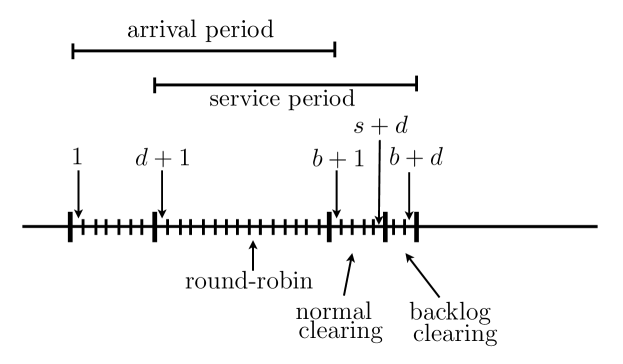
Figure 1: Illustration of a typical arrival period and the phases of a service period. Slots are numbered consecutively, starting with the first slot of the arrival period.

1. The first $b-d$ slots of the $k$th service period, namely, slots $kb+d+1,\ldots,(k+1)b$, comprise a round-robin phase: we cycle through the schedules ${\boldsymbol{\sigma}}^{(1)}$, ${\boldsymbol{\sigma}}^{(2)}$, …, ${\boldsymbol{\sigma}}^{(n)}$ in a round-robin manner. However, during this phase, we do not serve any of the backlogged packets; we only serve packets that belong to the $k$th batch.

2. The next $\ell=d+s-b$ slots, namely slots $(k+1)b+1,\ldots,kb+d+s$, comprise the $k$th normal clearing phase. Similar to the round-robin phase, we do not serve any backlogged packets during this phase. Furthermore, even though packets from the $(k+1)$st batch may have started to arrive, we do not serve any of them. By the beginning of this phase, all of the arrivals from the $k$th batch have already arrived. Some of them have already been served during the round-robin phase. To those that remain, we apply the optimal clearing policy described earlier; cf. Theorem 4.3. However, there is a possibility that the phase terminates before we succeed in serving all of the remaining packets from the $k$th batch. Let $U_{k}$ be the number of the packets from the $k$th batch that were left unserved during this phase. These $U_{k}$ packets are considered backlogged and are added to the backlog $B_{k}$ from earlier periods.

3. The last $r=b-s$ slots, namely slots $kb+d+s+1,\ldots,{(k+1)b+d}$, comprise the $k$th backlog clearing phase. During this phase, we serve backlogged packets using some arbitrary policy. The only requirement is that the policy serve at least one packet at each slot that a backlogged packet is available. However, we do not serve any of the newly arrived packets from the $(k+1)$st batch. Any backlogged packets that are not served during this phase remain backlogged and comprise the number $B_{k+1}$ of backlogged packets at the beginning of the next service period. Since at least one backlogged packet is served (whenever available) during each one of these $r$ slots, and since there are no additions to the backlog during this phase, we have

   $$B_{k+1}\leq\max\{0,B_{k}+U_{k}-r\},\qquad k=0,1,\ldots$$ (12)

The total length of the three phases is

$$(b-d)+(d+s-b)+(b-s)=b,$$

so that the length of a service period is equal to the length of an arrival period. However, before continuing, we need to make sure that the duration of each phase is a positive number, so that the policy is well-defined. This is accomplished in the next two lemmas, which also provide order of magnitude information on the durations of these phases.

Lemma 5.1.

The length $r=b-s$ of the backlog clearing phase satisfies

$$r=c_{r}f_{n}\log f_{n},$$

where $c_{r}=c_{b}-\sqrt{c_{s}c_{b}}>0$. In particular, when $n$ is large enough, we have $r\geq 1$.

Proof.

Using the assumption $\rho=1-1/f_{n}$, we have $(1-\rho)b=b/f_{n}=c_{b}f_{n}\log f_{n}$. We then obtain

$$b-s = b-\rho b-\sqrt{c_{s}b\log f_{n}}$$

$$= c_{b}f_{n}\log f_{n}-\sqrt{c_{s}c_{b}f_{n}^{2}\log^{2}f_{n}}$$

$$= (c_{b}-\sqrt{c_{s}c_{b}})f_{n}\log f_{n}$$

$$= c_{r}f_{n}\log f_{n}.$$

The fact that $c_{r}>0$ follows from our assumption in Eq. (11). ∎

Lemma 5.2.

The length $\ell=d+s-b$ of the normal clearing phase satisfies

$$\ell\geq c_{\ell}\sqrt{n}f_{n}\log f_{n},$$

where $c_{\ell}=c_{d}-c_{r}>0$. In particular, when $n$ is large enough, we have $\ell\geq 1$.

Proof.

Recall that $r=b-s$. It follows that

$$\ell = d+s-b$$

$$= d-r$$

$$= c_{d}\sqrt{n}f_{n}\log f_{n}-c_{r}f_{n}\log f_{n}$$

$$\geq (c_{d}-c_{r})\sqrt{n}f_{n}\log f_{n}$$

$$= c_{\ell}\sqrt{n}f_{n}\log f_{n}.$$

Note that $c_{r}<c_{b}<c_{d}$ (cf. Lemma 5.1 and Eq. (11)), which implies that $c_{\ell}>0$. ∎

6 Policy Analysis

The performance analysis of the proposed policy involves the following line of argument for what happens during the $k$th arrival and service period.

1. In the first $d$ slots of the $k$th arrival period, we have an expected number $O(nd)$ of arrivals.

2. With high probability, at every time slot during the round-robin phase, there is a positive number of packets from the $k$th arrival batch at each queue; cf. Lemmas 6.1 and 6.2. Therefore, offered service is never wasted. In particular, at least as many packets are served as they arrive (in the expected value sense), and the total queue size does not grow.

3. With high probability, all of the packets from the $k$th batch that are in queue at the beginning of the normal clearing phase get cleared and therefore the number $U_{k}$ of newly backlogged packets is zero; cf. Lemma 6.4.

4. The number $B_{k}$ of backlogged packets evolves similar to a discrete-time G/D/1 queue; cf. Eq. (12). Because $U_{k}$ is zero with high probability, the Kingman bound (Theorem 4.2) implies that the expected number of backlogged packets, at any time, is small; cf. Lemma 6.5.

The above steps, when translated into precise bounds on queue sizes, will lead to an $O(nd)$ bound on the expected total queue size at any time.

6.1 No waste during the round-robin phase

In this subsection, we establish that during the round-robin phase, every queue contains a nonzero number of packets from the current arrival batch, with high probability. We first introduce some convenient notation. We will use the variable $t\in\{1,\ldots,b+1\}$ to index the $b$ slots of the $k$th arrival period together with the first slot of the subsequent normal clearing phase. For $t\in\{1,\ldots,b\}$, we let $A_{i,j}^{k}(t)$ be the number of arrivals to the $(i,j)$th queue during the first $t$ time slots of the $k$th arrival period; these are the time slots $kb+1,kb+{2},\ldots,kb+t$. Similarly, for $t\in\{1,\ldots,b\}$, we let $S_{i,j}^{k}(t)$ be the number of packets that arrive to queue $(i,j)$ during the $k$th arrival period and get served during the first $t$ time slots of the $k$th arrival period. Finally, for $t\in\{1,\ldots,b+1\}$, we let $Q_{i,j}^{k}(t)$ be the number of packets from the $k$th arrival batch that are in queue $(i,j)$ at the beginning of the $t$th slot of the $k$th arrival period. With these definitions, we have,

$$Q^{k}_{i,j}(t+1)=A^{k}_{i,j}(t)-S^{k}_{i,j}(t),\qquad t=1,\ldots,b.$$ (13)

We are interested in conditions under which no offered service is wasted during the round-robin phase. Equivalently, we are interested in conditions under which all queues have a positive number of packets from the $k$th batch. Note that the round-robin phase involves slots for which $t\in\{d+1,\ldots,b\}$. We have the following observation on the queue sizes at the beginning of these slots.

Lemma 6.1.

Suppose that $t\in\{d,\ldots,b-1\}$ and that

$$A_{i,j}^{k}(t)>\frac{t-d}{n}+1.$$

Then, $Q^{k}_{i,j}(t+1)>0$.

Proof.

Note that that for the first $d$ time slots, packets from the $k$th batch do not receive any service. Starting from the $(d+1)$st slot, we are in the round-robin phase, and queue $(i,j)$ is offered service once every $n$ slots. Therefore,

$$S^{k}_{i,j}(t)\leq\Big{\lceil}\frac{t-d}{n}\Big{\rceil}<\frac{t-d}{n}+1<A_{i,j}^{k}(t).$$

The result follows from Eq. (13). ∎

The previous lemma highlights the importance of the events $A_{i,j}^{k}(t)>{(t-d)/n+1}$. We will show that the complements of these events have, collectively, small probability. To this effect, let $W_{i,j}^{k}(t)$ be the event defined by

$$W^{k}_{i,j}(t)=\Big{\{}A_{i,j}^{k}(t)\leq\frac{t-d}{n}+1\Big{\}},\qquad{t=d,\ldots,b-1.}$$

Let also $W^{k}$ be the union of these events, over all queues, and over all indices $t$ that are relevant to the round-robin phase:

$$W^{k}=\bigcup_{i=1}^{n}\bigcup_{j=1}^{n}\bigcup_{{t=d}}^{{b-1}}W^{k}_{i,j}(t).$$

Lemma 6.2.

For $n$ sufficiently large, we have

$$\mathbb{P}(W^{k})\leq\frac{1}{2f_{n}^{13}},\qquad\mbox{for all }k.$$

Proof.

Let us fix some $(i,j)$ and some $t\in\{d,\ldots,b{-1}\}$. Note that $\mathbb{E}\big{[}A_{i,j}^{k}(t)\big{]}=\rho t/n$. Therefore, the event $W_{i,j}^{k}(t)$ is the same as the event

$$\Big{\{}A_{i,j}^{k}(t)\leq\mathbb{E}\big{[}A_{i,j}^{k}(t)\big{]}-\frac{\rho t}{n}+\frac{t-d}{n}+1\Big{\}},$$

which is of the form

$$\Big{\{}A_{i,j}^{k}(t)\leq\mathbb{E}\big{[}A_{i,j}^{k}(t)\big{]}-x\Big{\}},$$

where

$$x = \frac{\rho t}{n}-\frac{t-d}{n}-1$$

$$= \frac{\rho(t-d)}{n}-\frac{t-d}{n}+\frac{\rho d}{n}-1$$

$$= -(1-\rho)\frac{t-d}{n}+\frac{\rho d}{n}-1.$$

Using the facts $t-d\leq b$ and $1-\rho=1/f_{n}$, the first term on the right-hand side is bounded above (in absolute value) by $b/(nf_{n})$. For the second term, we use the facts $\rho=1-(1/f_{n})$, $f_{n}\geq n\geq 2$, to obtain $\rho\geq 1/2$. Therefore,

$$x \geq -\frac{b}{nf_{n}}+\frac{d}{2n}-1$$

$$= \frac{1}{n}\Big{(}(c_{d}/2)\sqrt{n}f_{n}\log f_{n}-c_{b}f_{n}\log f_{n}-n\Big{)}$$

$$\geq \frac{1}{n}\Big{(}(c_{d}/2)\sqrt{n}f_{n}\log f_{n}-(c_{b}+1)f_{n}\log f_{n}\Big{)}.$$

Now, for $n$ large enough, we have $c_{b}+1\leq(c_{d}/4)\sqrt{n}$, and this implies that

$$x\geq\frac{1}{n}\cdot\frac{c_{d}}{4}\cdot\sqrt{n}f_{n}\log f_{n}=\frac{c_{d}f_{n}\log f_{n}}{4\sqrt{n}}.$$ (14)

Using Eq. (3) (the lower tail bound in Theorem 4.1), we have

$$\mathbb{P}\big{(}W_{i,j}^{k}(t)\big{)}=\mathbb{P}\Big{(}A_{i,j}^{k}(t)\leq\mathbb{E}\big{[}A_{i,j}^{k}(t)\big{]}-x\Big{)}\leq\exp\Big{\{}-\frac{x^{2}}{2\mathbb{E}[A_{i,j}^{k}(t)]}\Big{\}}.$$

We note that $\mathbb{E}[A_{i,j}^{k}(t)]=\rho t/n\leq b/n=c_{b}f_{n}^{2}(\log f_{n})/n$. Using also Eq. (14), we obtain

$$\frac{x^{2}}{2\mathbb{E}[A_{i,j}^{k}(t)]}\geq\frac{c_{d}^{2}f_{n}^{2}\log^{2}f_{n}}{16n}\cdot\frac{1}{2c_{b}f_{n}^{2}(\log f_{n})/n}=\frac{c_{d}^{2}}{32c_{b}}\log f_{n}\geq 20\log f_{n},$$

where the last inequality follows from our assumption that $c_{d}^{2}\geq 640c_{b}$; cf. Eq. (11). Consequently,

$$\mathbb{P}\big{(}W_{i,j}^{k}(t)\big{)}\leq\exp\{-20\log f_{n}\}=\frac{1}{f_{n}^{20}}\leq\frac{1}{2f_{n}^{19}}.$$

The event $W^{k}$ is the union of $n^{2}(b-d)$ events $W^{k}_{i,j}(t)$. We note that

$${n^{2}(b-d)}\leq n^{2}b\leq f_{n}^{2}c_{b}f_{n}^{2}\log f_{n}\leq f_{n}^{6},$$ (15)

as long as $n$ is large enough so that $c_{b}\leq f_{n}$. Therefore, using the union bound

$$\mathbb{P}(W^{k})\leq{n^{2}(b-d)}\frac{1}{2f_{n}^{19}}\leq\frac{f_{n}^{6}}{2f_{n}^{19}}=\frac{1}{2f_{n}^{13}}.$$

∎

6.2 The probability of no new backlog

In this subsection we show that $U_{k}$, the additional backlog generated during the $k$th service period, is zero with high probability. Our analysis builds on an upper bound on the probability that the number of packets in the $k$th batch that are associated with a particular port is appreciably larger than its expected value. Towards this purpose, we define the row and column sums for the arrivals in the $k$th batch:

$$R_{i}^{k}=\sum_{j}A^{k}_{i,j}(b),\qquad C_{j}^{k}=\sum_{i}A^{k}_{i,j}(b).$$

We also define the events

$$F_{i}^{k}=\{R_{i}^{k}>s\},\qquad G^{k}_{j}=\{C_{j}^{k}>s\},$$

and

$$H^{k}=\big{(}F_{1}^{k}\cup\cdots\cup F_{n}^{k}\big{)}\cup\big{(}G_{1}^{k}\cup\cdots\cup G_{n}^{k}\big{)}.$$

In what follows, we first show that the event $H^{k}$ has low probability. We then show that if neither of the events $W^{k}$ or $H^{k}$ occurs (which has high probability), then $U_{k}$ is equal to zero.

Lemma 6.3.

For $n$ sufficiently large, we have

$$\mathbb{P}(H^{k})\leq\frac{1}{2f_{n}^{13}},\qquad\mbox{for all }k.$$

Proof.

Let us focus on the event $F_{1}^{k}=\{R_{1}^{k}>s\}$; the argument for other events $F_{i}^{k}$ or $G_{j}^{k}$ is identical. Note that $\mathbb{E}[R_{1}^{k}]=\rho b$. We have, using Eq. (4) (the upper tail bound in Theorem 4.1) in the last step,

$$\mathbb{P}(R_{1}^{k}>s) = \mathbb{P}\big{(}R_{1}^{k}>\rho b+\sqrt{c_{s}b\log f_{n}}\big{)}$$

$$= \mathbb{P}\big{(}R_{1}^{k}>\mathbb{E}[R_{1}^{k}]+\sqrt{c_{s}b\log f_{n}}\big{)}$$

$$\leq \exp\Big{\{}-\frac{c_{s}b\log f_{n}}{2(\rho b+x/3)}\Big{\}},$$

where $x=\sqrt{c_{s}b\log f_{n}}$. Notice that

$$\rho b+\frac{x}{3}\leq\rho b+x=\rho b+\sqrt{c_{s}b\log f_{n}}=s\leq b.$$

Therefore, when $n\geq 4$,

$$\mathbb{P}(R_{1}^{k}>s)\leq\exp\Big{\{}-\frac{c_{s}b\log f_{n}}{2b}\Big{\}}=\frac{1}{f_{n}^{c_{s}/2}}\leq\frac{1}{4f_{n}^{14}},$$

where the last inequality follows from our assumption that $c_{s}\geq 30$; cf. Eq. (11). The event $H^{k}$ is the union of $2n$ events, each with probability bounded above by $1/(4f_{n}^{14})$. Using the union bound and the assumption $n\leq f_{n}$, we obtain $\mathbb{P}(H^{k})\leq 1/(2f_{n}^{13})$. ∎

Lemma 6.4.

1. Consider a sample path under which neither $W^{k}$ nor $H^{k}$ occurs. Then, $U_{k}=0$.

2. We have $\mathbb{P}(U_{k}>0)\leq 1/f_{n}^{13}$.

3. For every sample path, we have $U_{k}\leq n^{2}b$.

Proof.

• We assume that neither $W^{k}$ nor $H^{k}$ occurs. Using Eq. (13), the queue sizes (where we only count packets from the $k$th batch) at the beginning of the normal clearing period are equal to

  $$Q^{k}_{i,j}(b+1)=A_{i,j}^{k}(b)-S^{k}_{i,j}(b).$$ (16)

  Let

  $$\hat{R}_{i}^{k}=\sum_{j}Q^{k}_{i,j}(b+1),\qquad\hat{C}_{j}^{k}=\sum_{i}Q^{k}_{i,j}(b+1).$$

  Now consider a fixed $i$. Note that the schedules ${\boldsymbol{\sigma}}^{(m)}$ used during the round-robin phase have the property $\sum_{j}\sigma_{i,j}^{(m)}=1$; that is, each input port is offered exactly one unit of service at each time slot. Furthermore, since event $W^{k}$ does not occur, Lemma 6.1 implies that all queues are positive at the beginning of each slot of the round-robin phase; that is, $Q^{k}_{ij}(t+1)>0$, for $t=d,\ldots,b-1$. Therefore, the offered service is never wasted during the $b-d$ slots of the round-robin phase. It follows that the total actual service at input port $i$ during the round-robin phase is exactly $b-d$:

  $$\sum_{j}S_{i,j}^{k}(b)=b-d.$$

  Furthermore, since event $H^{k}$ does not occur, we have $R_{i}^{k}\leq s$. Recalling the definition $R_{i}^{k}=\sum_{j}A_{i,j}^{k}(b)$, and by summing both sides of Eq. (16) over all $j$, we obtain

  $$\hat{R}_{i}^{k}=R_{i}^{k}-\sum_{j}S_{i,j}^{k}(b)\leq s-(b-d)=\ell,$$

  where $\ell=d+s-b$ is the length of the normal clearing phase. By a similar argument, we obtain that $\hat{C}_{j}^{k}\leq\ell$, for all $j$. It then follows from Theorem 4.3 that all the packets (from the $k$th arrival batch) will be cleared during the normal clearing phase, and $U_{k}=0$.

• If $U_{k}>0$, then, by part (a), it must be that either event $W^{k}$ or $H^{k}$ occurs. The result follows because the probability of each one of these two events is upper bounded by $1/(2f_{n}^{13})$ (Lemmas 6.2 and 6.3).

• The number of packets from the $k$th batch that can get backlogged can be no more than the total number of arrivals in the $k$th batch. Since each queue ($n^{2}$ of them) receives at most one packet at each time slot ($b$ slots), the total number cannot exceed $n^{2}b$.

∎

6.3 Backlog analysis

We are now in a position to show that the expected backlog is very small.

Lemma 6.5.

Assuming that $n$ is sufficiently large, we have that $\mathbb{E}[B_{k}]\leq 1$, for all $k$.

Proof.

Using Eq. (12), the backlog satisfies

$$B_{k+1}\leq\max\{0,B_{k}+U_{k}-r\}\leq\max\{0,B_{k}+U_{k}-1\}.$$

Let us define a sequence $\hat{B}_{k}$ with the recursion $\hat{B}_{0}=0$ and

$$\hat{B}_{k+1}=\max\{0,\hat{B}_{k}+U_{k}-1\}.$$

We then have $B_{k}\leq\hat{B}_{k}$, so it suffices to derive an upper bound on $\mathbb{E}[\hat{B}_{k}]$.

We use the discrete-time Kingman bound (Theorem 4.2), where we identify $Z(\tau)$ with $\hat{B}_{k}$, $X(\tau)$ with $U_{k}$, and $Y(\tau)$ with 1. Using the notation in Theorem 4.2, we have $\mu=1$, and $m_{2y}=1$. Furthermore, as in Eq. (15), we have $n^{2}b\leq f_{n}^{6}$ for sufficiently large $n$. Using Lemma 6.4,

$$\lambda=\mathbb{E}[U_{k}]\leq f_{n}^{6}\cdot\mathbb{P}(U_{k}>0)\leq f_{n}^{6}\cdot\frac{1}{f_{n}^{13}}=\frac{1}{f_{n}^{7}},$$

and

$$m_{2x}=\mathbb{E}[U_{k}^{2}]\leq f_{n}^{12}\cdot\mathbb{P}(U_{k}>0)=f_{n}^{12}\cdot\frac{1}{f_{n}^{13}}=\frac{1}{f_{n}}.$$

Then, using the bound in (6), we have

$$\mathbb{E}[B_{k}]\leq\mathbb{E}[\hat{B}_{k}]\leq\frac{m_{2x}+m_{2y}}{2(\mu-\lambda)}\leq\frac{f_{n}^{-1}+1}{2(1-f_{n}^{-7})}.$$

As $n$ increases, the right-hand side converges to $1/2$ and is therefore bounded above by $1$ when $n$ is sufficiently large. ∎

6.4 Queue size analysis

In this subsection we show that at any time, the sum of the queue sizes is of order $O(nd)$. We fix some time $\tau$ and consider two cases, depending on whether this time belongs to a round-robin phase or not.

Queue sizes during the round-robin phase

Suppose that $\tau$ satisfies $kb+d+1\leq\tau\leq(k+1)b$, so that $\tau$ belongs to the round-robin phase of the $k$th service period, and let us look at the queue size $Q_{i,j}(\tau+1)$. This queue size may include some packets that arrived during earlier arrival periods and that were backlogged; their total expected number (summed over all $i$ and $j$) is $\mathbb{E}[B_{k}]\leq 1$.

Let us now turn our attention to packets that belong to the $k$th batch. Recall that the number of such packets in queue $(i,j)$ at the beginning of the $(t+1)$st slot (equivalently, the end of the $t$th slot) of the $k$th arrival period is denoted by $Q^{k}_{i,j}(t+1)$. For $t=d+1,\ldots,b$, we have, as in Eq. (13),

$$Q^{k}_{i,j}(t+1)=A^{k}_{i,j}(t)-S_{i,j}^{k}(t),$$

and

$$\sum_{i,j}\mathbb{E}[Q^{k}_{i,j}(t+1)]=n\rho t-\mathbb{E}\Big{[}\sum_{i,j}S_{i,j}^{k}(t)\Big{]}.$$

By the same argument as in the proof of Lemma 6.4(a), if event $W^{k}$ does not occur, the service during the round-robin phase is never wasted: a total of $n$ packets are served at each time, and for $t=d+1,\ldots,b$, a total of $n(t-d)$ packets are served by the $t$th slot of the $k$th arrival period. Using also the inequality (cf. Lemma 6.2)

$$1-\mathbb{P}({W^{k}})\geq 1-\frac{1}{{2}f_{n}^{13}}\geq 1-\frac{1}{f_{n}}=\rho,$$

we obtain

$$\mathbb{E}\Big{[}\sum_{i,j}S_{i,j}^{k}(t)\Big{]}\geq n(t-d)\big{(}1-\mathbb{P}({W^{k}})\big{)}\geq n\rho(t-d).$$

Therefore,

$$\sum_{i,j}\mathbb{E}[Q^{k}_{i,j}(t+1)]\leq n\rho t-n\rho(t-d)=n\rho d\leq nd,\qquad t=d+1,\ldots,b.$$ (17)

which is an upper bound of the desired form.

Queue sizes outside the round-robin phase

Suppose now that $\tau$ satisfies $(k+1)b+1\leq\tau\leq(k+1)b+d$, so that $\tau$ belongs to one of the last two phases of the $k$th service period, and let us look again at the queue size $Q_{i,j}(\tau+1)$. As before, we may have some backlogged packets. These are either packets backlogged during the current period (the $k$th one) or in previous periods. Their total expected number (summed over all $i$ and $j$) at any time in this range is upper bounded by $\mathbb{E}[B_{k}+U_{k}]\leq 2$.

Let us now turn our attention to packets that belong to the $k$th batch. Since there are no further arrivals from the $k$th batch from slot $(k+1)b+1$ onwards, the number of such packets is largest at the beginning of slot $(k+1)b+1$. Their expected value at that time satisfies

$$\sum_{i,j}\mathbb{E}\big{[}Q^{k}_{i,j}(b+1)\big{]}\leq nd,$$

where in the inequality we used Eq. (17) with $t=b$.

Finally, we need to account for arrivals that belong to the $(k+1)$st arrival batch. The total number of such accumulated arrivals is largest when we consider the largest value of $\tau$, namely, $\tau=(k+1)b+d$. By that time, we have had a total of $d$ slots of the $(k+1)$st arrival period, and a total expected number of arrivals equal to $\rho nd$, which is bounded above by $nd$.

Putting together all of the bounds that we have developed, we see that at any time, the expected total number of packets is bounded above by $2nd+2\leq 3nd$. This being true for all sufficiently large $n$, establishes Theorem 3.1.

7 Discussion

We presented a novel scheduling policy for an $n\times n$ input-queued switch. In the regime where the system load satisfies $\rho=1-1/n$, and the arrival rates at the different queues are all equal, our policy achieves an upper bound of order $O(n^{2.5}\log n)$ on the expected total queue size, a substantial improvement upon earlier upper bounds, all of which were of order $O(n^{3})$, ignoring poly-logarithmic dependence on $n$. Our policy is of the batching type. However, instead of waiting until an entire batch has arrived, our policy only waits for enough arrivals to take place for the system to exhibit a desired level of regularity, and then starts serving the batch. This idea may be of independent interest.

Our policy uses detailed knowledge of the arrival statistics, and is heavily dependent on the fact that all arrival rates are the same. While we believe that similar policies can be devised for arbitrary arrival rates (within the regime considered in this paper), the policy description and analysis are likely to be more involved.

Finally, for the regime where $\rho\approx 1-1/n$, there is a $\Omega(n^{2})$ lower bound on the expected total queue size under any policy (see [13]), whereas our upper bound is of order $O(n^{2.5}\log n)$. It is an interesting open question whether this gap between the upper and lower bound can be closed. Our policy uses a prespecified sequence of schedules (round-robin) until the entire batch has arrived and then uses an “adaptive” sequence of schedules to clear remaining packets after the end of the batch. Within the class of policies of this type, with perhaps different choices of the parameters involved, it appears to be impossible to obtain an upper bound of $O(n^{\alpha})$ for $\alpha<2.5$. Thus, in order to come closer to the $\Omega(n^{2})$ lower bound, we will have to use an adaptive sequence of schedules early on, before the entire batch has arrived. In fact, if one were to achieve an upper bound close to $O(n^{2})$, we would have an approximately constant expected number of packets in each queue. This means that with positive probability, many of the queues will be empty. Therefore, an elaborate policy would be needed to avoid offering service to empty queues and thus avoid queue buildup. But the analysis of such elaborate policies appears to be a difficult challenge.

References

- [1] F. Chung. Complex graphs and networks. American Mathematical Society (2006)
- [2] J. G. Dai and B. Prabhakar. The throughput of switches with and without speed-up. Proceedings of IEEE Infocom, pp. 556–564 (2000)
- [3] M. Jr. Hall. Combinatorial theory. Wiley-Interscience, 2nd edition (1998)
- [4] J. M. Harrison. Brownian models of open processing networks: canonical representation of workload. The Annals of Applied Probability 10, 75–103 (2000). URL http://projecteuclid.org/euclid.aoap/1019737665. Also see [5]
- [5] J. M. Harrison. Correction to [4]. The Annals of Applied Probability 13, 390–393 (2003)
- [6] F. P. Kelly and R. J. Williams. Fluid model for a network operating under a fair bandwidth-sharing policy. The Annals of Applied Probability 14, 1055–1083 (2004)
- [7] I. Keslassy and N. McKeown. Analysis of scheduling algorithms that provide 100% throughput in input-queued switches. Proceedings of Allerton Conference on Communication, Control and Computing (2001)
- [8] E. Leonardi, M. Mellia, F. Neri and M. A. Marsan. Bounds on average delays and queue size averages and variances in input queued cell-based switches. Proceedings of IEEE Infocom, pp. 1095–1103 (2001)
- [9] W. Lin and J. G. Dai. Maximum pressure policies in stochastic processing networks Operations Research, 53, 197–218 (2005)
- [10] N. McKeown, V. Anantharam and J. Walrand. Achieving 100% throughput in an input-queued switch. Proceedings of IEEE Infocom, pp. 296–302 (1996)
- [11] M. Neely, E. Modiano and Y. S. Cheng. Logarithmic delay for packet switches under the cross-bar constraint. IEEE/ACM Transactions on Networking 15(3) (2007)
- [12] D. Shah and M. Kopikare. Delay bounds for the approximate Maximum Weight matching algorithm for input queued switches. Proceedings of IEEE Infocom (2002)
- [13] D. Shah, J. N. Tsitsiklis and Y. Zhong. Optimal scaling of average queue sizes in an input-queued switch: an open problem. Queueing Systems 68(3-4), 375–384 (2011)
- [14] D. Shah, N. Walton and Y. Zhong. Optimal queue-size scaling in switched networks. Accepted to appear in the Annals of Applied Probability (2014)
- [15] R. Srikant and L. Ying. Communication networks: An optimization, control and stochastic networks perspective. Cambridge University Press (2014)
- [16] L. Tassiulas and A. Ephremides. Stability properties of constrained queueing systems and scheduling policies for maximum throughput in multihop radio networks. IEEE Transactions on Automatic Control 37, 1936–1948 (1992)
- [17] G. de Veciana, T. Lee and T. Konstantopoulos. Stability and performance analysis of networks supporting elastic services. IEEE/ACM Transactions on Networking 9(1), 2–14 (2001)