E P

Stefan Magureanu magur@kth.se
KTH, The Royal Institute of Technology, EE School / ACL, Osquldasv. 10, Stockholm 100-44, Sweden and Richard Combesrichard.combes@supelec.fr
Supelec, Plateau de Moulon, 3 rue Joliot-Curie 91192 Gif-sur-Yvette Cedex, France and Alexandre Proutiere alepro@kth.se
KTH, The Royal Institute of Technology, Stockholm, Sweden, and INRIA, Paris, France

Lipschitz Bandits:
Regret Lower Bounds and Optimal Algorithms

We consider stochastic multi-armed bandit problems where the expected reward is a Lipschitz function of the arm, and where the set of arms is either discrete or continuous. For discrete Lipschitz bandits, we derive asymptotic problem specific lower bounds for the regret satisfied by any algorithm, and propose OSLB and CKL-UCB, two algorithms that efficiently exploit the Lipschitz structure of the problem. In fact, we prove that OSLB is asymptotically optimal, as its asymptotic regret matches the lower bound. The regret analysis of our algorithms relies on a new concentration inequality for weighted sums of KL divergences between the empirical distributions of rewards and their true distributions. For continuous Lipschitz bandits, we propose to first discretize the action space, and then apply OSLB or CKL-UCB, algorithms that provably exploit the structure efficiently. This approach is shown, through numerical experiments, to significantly outperform existing algorithms that directly deal with the continuous set of arms. Finally the results and algorithms are extended to contextual bandits with similarities.

1 Introduction

In their seminal paper, [lai1985] solve the classical stochastic Multi-Armed Bandit (MAB) problem. In this problem, the successive rewards of a given arm are i.i.d., and the expected rewards of the various arms are not related. They derive an asymptotic (when the time horizon grows large) lower bound of the regret satisfied by any algorithm, and present an algorithm whose regret matches this lower bound. This initial algorithm was quite involved, and many researchers have, since then, tried to devise simpler and yet efficient algorithms. The most popular of these algorithms are UCB [auer2002] and its extensions, e.g. KL-UCB [garivier2011], [cappe2012] – note that the KL-UCB algorithm was initially proposed and analysed in [lai1987], see (2.6). When the expected rewards of the various arms are not related as in [lai1985], the regret of the best algorithm essentially scales as $O(K\log(T))$ where $K$ denotes the number of arms, and $T$ is the time horizon. When $K$ is very large or even infinite, MAB problems become more challenging. Fortunately, in such scenarios, the expected rewards often exhibit some structural properties that the decision maker can exploit to design efficient algorithms. Various structures have been investigated in the literature, e.g., Lipschitz [agrawal95], [kleinberg2008], [bubeck08], linear [dani08], and convex [kalai05].

In this paper, we revisit bandit problems where the expected reward is a Lipschitz function of the arm. The set of arms is a subset of $[0,1]$ and we address both discrete Lipschitz bandits where this set is finite, and continuous Lipschitz bandits where this set is [0,1]. For discrete Lipschitz bandits, we derive problem specific regret lower bounds, and propose OSLB (Optimal Sampling for Lipschitz Bandits), an algorithm whose regret matches our lower bound. Most previous work on Lipschitz bandit problems address the case where the set of arms is [0,1], [agrawal95], [kleinberg2008], [bubeck08]. For these problems, there is no known problem specific regret lower bound. In [kleinberg2008], a regret lower bound is derived for the worst Lipschitz structure. The challenge in the design of efficient algorithms for continuous Lipschitz bandits stems from the facts that such algorithms should adaptively select a subset of arms to sample from, and based on the observed samples, establish tight confidence intervals and construct arm selection rules that optimally exploit the Lipschitz structure revealed by past observations. The algorithms proposed in [agrawal95], [kleinberg2008], [bubeck08] adaptively define the set of arms to play, but used simplistic UCB indexes to sequentially select arms. In turn, these algorithms fail at exploiting the problem structure revealed by the past observed samples. For continuous bandits, we propose to first discretize the set of arms (as in [kleinberg2008]), and then apply OSLB, an algorithm that optimally exploits past observations and hence the problem specific structure. As it turns out, this approach outperforms algorithms directly dealing with continuous sets of arms.

Our contributions.

(a) For discrete Lipschitz bandit problems, we derive an asymptotic regret lower bound satisfied by any algorithm. This bound is problem specific in the sense that it depends in an explicit manner on the expected rewards of the various arms (this contrasts with existing lower bounds for continuous Lipschitz bandits).

(b) We propose OSLB (Optimal Sampling for Lipschitz Bandits), an algorithm whose regret matches our lower bound. We further present CKL-UCB (Combined KL-UCB), an algorithm that exhibits lower computational complexity than that of OSLB, and that is yet able to exploit the Lipschitz structure.

(c) We provide a finite time analysis of the regret achieved under OSLB and CKL-UCB. The analysis relies on a new concentration inequality for a weighted sum of KL divergences between the empirical distributions of rewards and their true distributions. We believe that this inequality can be instrumental for various bandit problems with structure.

(d) We evaluate our algorithms using numerical experiments for both discrete and continuous sets of arms. We compare their performance to that obtained using existing algorithms for continuous bandits.

(e) We extend our results and algorithms to the case of contextual bandits with similarities as investigated in [slivkins11].

2 Models

We consider a stochastic multi-armed bandit problem where the set of arms is a subset $\{x_{1},\ldots,x_{K}\}$ of the interval $[0,1]$. Results can be easily extended to the case where the set of arms is a subset of a metric space as considered in [kleinberg2008]. The set of arms is of finite cardinality, possibly large, and we assume without loss of generality that $x_{1}<x_{2}<\ldots<x_{K}$. Problems with continuous sets of arms are discussed in Section LABEL:sec:num. Time proceeds in rounds indexed by $n=1,2,\ldots$. At each round, the decision maker selects an arm, and observes the corresponding random reward. Arm $x_{k}$ is referred to as arm $k$ for simplicity. For any $k$, the reward of arm $k$ in round $n$ is denoted by $X_{k}(n)$, and the sequence of rewards $(X_{k}(n))_{n\geq 1}$ is i.i.d. with Bernoulli distribution of mean $\theta_{k}$ (the results can be generalized to distributions belonging to a certain parametrized family of distributions, but to simplify the presentation, we restrict our attention to Bernoulli rewards). The vector $\theta=(\theta_{1},\ldots,\theta_{K})$ represents the expected rewards of the various arms. Let ${\cal K}=\{1,\ldots,K\}$. We denote by $\theta^{\star}=\max_{k\in{\cal K}}\theta_{k}$ the expected reward of the best arm. A sequential selection algorithm $\pi$ selects in round $n$ an arm $k^{\pi}(n)\in{\cal K}$ that depends on the past observations. In other words, for any $n\geq 1$, if ${\cal F}_{n}^{\pi}$ denotes the $\sigma$-algebra generated by $(k^{\pi}(t),X_{k^{\pi}(t)}(t))_{1\leq t\leq n}$, then $k^{\pi}(n+1)$ is ${\cal F}_{n}^{\pi}$-measurable. Let $\Pi$ denote the set of all possible sequential selection algorithms.

We assume that the expected reward is a Lipschitz function of the arm, and this structure is known to the decision maker. More precisely, there exists a positive constant $L$ such that for all pairs of arms $(k,k^{\prime})\in{\cal K}$,

$$|\theta_{k}-\theta_{k^{\prime}}|\leq L\times|x_{k}-x_{k^{\prime}}|.$$ (1)

We assume that $L$ is also known. We denote by $\Theta_{L}$ the set of vectors in $[0,1]^{K}$ satisfying (1). The objective is to devise an algorithm $\pi\in\Pi$ that maximizes the average cumulative reward up to a certain round $T$ referred to as the time horizon ($T$ is typically large). Such an algorithm should optimally exploit the Lipschitz structure of the problem. As always in bandit optimization, it is convenient to quantify the performance of an algorithm $\pi\in\Pi$ through its expected regret (or regret for short) defined by:

$$R^{\pi}(T)=T\theta^{\star}-\mathbb{E}[\sum_{n=1}^{T}X_{k^{\pi}(n)}(n)].$$

3 Regret Lower Bound

In this section, we derive an asymptotic (when $T$ grows large) regret lower bound satisfied by any algorithm $\pi\in\Pi$. We denote by $I(x,y)=x\log({x\over y})+(1-x)\log({1-x\over 1-y})$ the KL divergence between two Bernoulli distributions with respective means $x$ and $y$. Fix the average reward vector $\theta=(\theta_{1},\ldots,\theta_{K})$. Let ${\cal K}^{-}=\{k\in{\cal K}:\theta_{k}<\theta^{\star}\}$ be the set of sub-optimal arms. For any $k\in{\cal K}^{-}$, we define $\lambda^{k}=(\lambda_{1},\ldots,\lambda_{K})$ as: $\forall i\in{\cal K},\quad\lambda^{k}_{i}=\max\{\theta_{i},\theta^{\star}-L|x_{k}-x_{i}|\}$. The expected reward vector $\lambda^{k}$ is illustrated in Figure 1, and may be interpreted as the most confusing reward vector among vectors in $\Theta_{L}$ such that arm $k$ (which is sub-optimal under $\theta$) is optimal under $\lambda^{k}$. This interpretation will be made clear in the proof of the following theorem. Without loss of generality, we restrict our attention to so-called uniformly good algorithms, as defined in [lai1985]. $\pi\in\Pi$ is uniformly good if for all $\theta\in\Theta_{L}$, $R^{\pi}(T)=o(T^{a})$ for all $a>0$. Uniformly good algorithms exist – for example, the UCB algorithm is uniformly good.

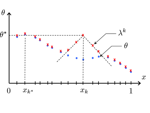
Figure 1: A Lipschitz bandit with 17 arms, and an example of sub-optimal expected reward vector $\lambda^{k}$ involved in the regret lower bound.

Theorem 3.1.

Let $\pi\in\Pi$ be a uniformly good algorithm. For any $\theta\in\Theta_{L}$, we have:

$$\lim\inf_{T\to\infty}{R^{\pi}(T)\over\log(T)}\geq C(\theta),$$ (2)

where $C(\theta)$ is the minimal value of the following optimization problem:

$$\min_{c_{k}\geq 0,\forall k\in{\cal K}^{-}}\sum_{k\in{\cal K}^{-}}c_{k}\times(\theta^{\star}-\theta_{k})$$ (3)

$$\hbox{s.t. }\forall k\in{\cal K}^{-},\ \sum_{i\in{\cal K}}c_{i}I(\theta_{i},\lambda^{k}_{i})\geq 1.$$ (4)

The regret lower bound is a consequence of results in optimal control of Markov chains, see [graves1997]. All proofs are presented in appendix. As in classical bandits, the minimal regret scales logarithmically with the time horizon. Observe that the lower bound (2) is smaller than the lower bound derived in [lai1985] when the various average rewards $(\theta_{k},k\in{\cal K})$ are not related (i.e., in absence of the Lipschitz structure). Hence (2) quantifies the gain one may expect by designing algorithms optimally exploiting the structure of the problem. Note that for any $k\in{\cal K}^{-}$, the variable $c_{k}$ corresponding to a solution of (3) characterizes the number of times arm $k$ should be played under an optimal algorithm: arm $k$ should be roughly played $c_{k}\log(n)$ times up to round $n$.

It should be also observed that our lower bound is problem specific (it depends on $\theta$), which contrasts with existing lower bounds for continuous Lipschitz bandits, see e.g. [kleinberg2008]. The latter are typically derived by selecting the problems that yield maximum regret. However, our lower bound is only valid for bandits with a finite set of arms, and cannot easily be generalized to problems with continuous sets of arms.

4 Algorithms

In this section, we present two algorithms for discrete Lipschitz bandit problems. The first of these algorithms, referred to as OSLB (Optimal Sampling for Lipschitz Bandits), has a regret that matches the lower bound derived in Theorem 3.1, i.e., it is asymptotically optimal. OSLB requires that in each round, one solves an LP similar to (3). The second algorithm, CKL-UCB (Combined KL-UCB) is much simpler to implement, but has weaker theoretical performance guarantees, although it provably exploits the Lipschitz structure.

4.1 The OSLB Algorithm

To formally describe OSLB, we introduce the following notations. For any $n\geq 1$, let $k(n)$ be the arm selected under OSLB in round $n$. $t_{k}(n)$ denotes the number of times arm $k$ has been selected up to round $n-1$. By convention, $t_{k}(1)=0$. The empirical reward of arm $k$ at the end of round $(n-1)$ is $\hat{\theta}_{k}(n)={1\over t_{k}(n)}\sum_{t=1}^{n-1}{\bf 1}\{k(t)=k\}X_{k}(t)$, if $t_{k}(n)>0$ and $\hat{\theta}_{k}(n)=0$ otherwise. We denote by $L(n)=\arg\max_{k\in{\cal K}}\hat{\theta}_{k}(n)$ the arm with the highest empirical reward (ties are broken arbitrarily) at the end of round $n-1$. Arm $L(n)$ is referred to as the leader for round $n$. We also define $\hat{\theta}^{\star}(n)=\hat{\theta}_{L(n)}(n)$ as the empirical reward of the leader at the end of round $n-1$. Let $f(n)=\log(n)+(3K+1)\log\log(n)$. Further define, for all $q\geq 0$ and $k$, the Lipschitz vector $\lambda^{q,k}$ such that for any $k^{\prime}$, $\lambda_{k^{\prime}}^{q,k}=q-L|x_{k}-x_{k^{\prime}}|$. The sequential decisions made under OSLB are based on the indexes of the various arms. The index $b_{k}(n)$ of arm $k$ for round $n$ is defined by:

$$b_{k}(n)=\sup\{q\in[\hat{\theta}_{k}(n),1]:\\ \sum_{k^{\prime}=1}^{K}t_{k^{\prime}}(n)I^{+}(\hat{\theta}_{k^{\prime}}(n),\lambda_{k^{\prime}}^{q,k})\leq f(n)\}.$$

Note that the index $b_{k}(n)$ is always well defined, even for small values of $n$, e.g. $n=1$ (we have for all $x>0$, $I^{+}(0,x)=-\log(1-x)$). For any $\theta\in\Theta_{L}$, let $C(\theta)$ denote the minimal value of the optimization problem (3), and let $(c_{k}(\theta),k\in{\cal K}^{-})$ be the values of the variables $(c_{k},k\in{\cal K}^{-})$ in (3) yielding $C(\theta)$. For simplicity, we define $\hat{C}(n)=C(\hat{\theta}(n))$, and $\hat{c}_{k}(n)=c_{k}(\hat{\theta}(n))$ for any $k\in{\cal K}^{-}(n)$ where ${\cal K}^{-}(n)=\{k:\hat{\theta}_{k}(n)<\hat{\theta}^{\star}(n)\}$. The design of OSLB stems from the observation that an optimal algorithm should satisfy $\lim_{n\to\infty}t_{k}(n)/(c_{k}(\theta)\log(n))=1$, almost surely, for all $k\in{\cal K}^{-}$. Hence we should force the exploration of arm $k\in{\cal K}^{-}(n)$ in round $n$ if $t_{k}(n)<\hat{c}_{k}(n)\log(n)$. We define the arm $\overline{k}(n)$ to explore as $\overline{k}(n)=\arg\min_{k\in K_{e}(n)}t_{k}(n)$ where $K_{e}(n)=\{k\in{\cal K}^{-}(n):t_{k}(n)\leq\hat{c}_{k}(n)\log(n)\}$. If $K_{e}(n)=\emptyset$, $\overline{k}(n)=-1$ (a dummy arm). Finally we define the least played arm as $\underline{k}(n)=\arg\min_{k}t_{k}(n)$. In the definitions of $\overline{k}(n)$ and $\underline{k}(n)$, ties are broken arbitrarily. We are now ready to describe OSLB. Its pseudo-code is presented in Algorithm 1.

Algorithm 1 OSLB($\epsilon$)

  For all $n\geq 1$, select arm $k(n)$ such that:

  If $\hat{\theta}^{\star}(n)\geq\max_{k\neq L(n)}b_{k}(n)$, then $k(n)=L(n)$;

  Else If $t_{\underline{k}(n)}(n)<{\epsilon\over K}t_{\overline{k}(n)}(n)$, then $k(n)=\underline{k}(n)$;

         Else $k(n)=\overline{k}(n)$.

Under OSLB, the leader is selected if its empirical average exceeds the index of other arms. If this is not the case, OSLB selects the least played arm $\underline{k}(n)$, if the latter has not been played enough, and arm $\overline{k}(n)$ otherwise. Note that the description of OSLB is valid in the sense that $\overline{k}(n)\neq-1$ if $\hat{\theta}^{\star}(n)<\max_{k\neq L(n)}b_{k}(n)$. After each round, all variables are updated, and in particular $\hat{c}_{k}(n)$ for any $k\in{\cal K}^{-}(n)$, which means that at each round we solve an LP, similar to (3).

4.2 The CKL-UCB Algorithm

Next, we present the algorithm CKL-UCB (Combined KL - UCB). The sequential decisions made under CKL-UCB are based on the indexes $b_{k}(n)$, and CKL-UCB explores the apparently suboptimal arms by choosing the least played arms first. When the leader $L(n)$ has the largest index, it is played, and otherwise we play the arm in $\{k:b_{k}(n)>b_{L(n)}(n)\}$, the set of arms which are possibly better than the leader, with the least number of current plays. Note that in practice, the forced $\log\log(n)$ exploration is unnecessary and only appears to aide in the regret analysis.

The rationale behind CKL-UCB is that if we are given a set of suboptimal arms, by exploring them, we will first eliminate arms whose expected reward is low (these arms do not require many plays to be eliminated). Note that the arm chosen by CKL-UCB is directly computed from the indexes, without solving an LP, and hence CKL-UCB is computationally light. From a practical perspective, CKL-UCB should also be more robust than OSLB in the sense that it does not take decisions based on the solution of the LP calculated with empirical averages $\hat{\theta}(n)$. This could be problematic if the LP solution is very sensitive to errors in the estimate of $\theta$.

Algorithm 2 CKL-UCB

  For all $n\geq 1$, select arm $k(n)$ such that:

  If $\exists k$ such that $t_{k}(n)<\log\log(n)$, then k(n) = k (ties are broken arbitrarily);

  Else if $b_{L(n)}(n)\geq\max\limits_{k\neq L(n)}b_{k}(n)$, then $k(n)=L(n)$;

         Else $k(n)=\arg\min\limits_{k}\{t_{k}(n):b_{k}(n)>b_{L(n)}(n)\}$ (ties are broken arbitrarily).

5 Regret Analysis

In this section, we provide finite time upper bounds for the regret achieved under OSLB and CKL-UCB.

5.1 Concentration Inequalities

To analyse the regret of algorithms for bandit optimization problems, one often has to leverage results related to the concentration-of-measure phenomenon. More precisely, here, in view of the definition of the indexes $b_{k}(n)$, we need to establish a concentration inequality for a weighted sum of KL divergences between the empirical distributions of rewards and their true distributions. We derive such an inequality. The latter extends to the multi-dimensional case the concentration inequality derived in [Garivier2013] for a single KL divergence. We believe that this inequality can be instrumental in the analysis of general structured bandit problems, as well as for statistical tests involving vectors whose components have distributions in a one-parameter exponential family (such as Bernoulli or Gaussian distributions). For simplicity, the inequality is stated for Bernoulli random variables only.

We use the following notations. For $k\in{\cal K}$, let $\{X_{k}(n)\}_{n\in\mathbb{N}}$ be a sequence of i.i.d. Bernoulli random variables with expectation $\theta_{k}$ and $X(n)=(X_{k}(n),k\in{\cal K})$. We represent the history up to round $n$ using the $\sigma$-algebra ${\cal F}_{n}=\sigma(X(1),\dots,X(n))$, and define the natural filtration ${\cal F}=\{{\cal F}_{n}\}_{n\geq 1}$. We consider a generic sampling rule $B(n)=(B_{k}(n),k\in{\cal K})$ where $B_{k}(n)\in\{0,1\}$ for all $k\in{\cal K}$. The sampling rule is assumed to be predictable in the sense that $B(n)\in{\cal F}_{n-1}$.

We define the number of times that $k$ was sampled up to round $n-1$ by $t_{k}(n)=\sum_{t=1}^{n-1}B_{k}(t)$ and the sum $S_{k}(n)=\sum_{t=1}^{n-1}B_{k}(t)X_{k}(t)$. The empirical average for $k$ is $\hat{\theta}_{k}(n)=S_{k}(n)/t_{k}(n)$ if $t_{k}(n)>0$ and $\hat{\theta}_{k}(n)=0$ otherwise. Finally, we define the vectors $\hat{\theta}(n)=(\hat{\theta}_{1}(n),\dots,\hat{\theta}_{K}(n))$ and $t(n)=(t_{1}(n),\dots,t_{K}(n))$. When comparing vectors in $\mathbb{R}^{K}$, we use the component-by-component order unless otherwise specified.

Theorem 5.1.

For all $\delta\geq(K+1)$ and $n\in\mathbb{N}$ we have:

$$\mathbb{P}\left[\sum_{k=1}^{K}t_{k}(n)I^{+}(\hat{\theta}_{k}(n),\theta_{k})\geq\delta\right]\leq e^{-\delta}\left(\frac{\lceil\delta\log(n)\rceil\delta}{K}\right)^{K}e^{K+1}.$$ (5)

The proof of Theorem 5.1 involves tools that are classically used in the derivation of concentration inequalities, but also requires the use of stochastic ordering techniques, see e.g. [MullerStoyan].

5.2 Finite time analysis of OSLB

Next we provide a finite time analysis of the regret achieved under OSLB, under the following mild assumption. This assumption greatly simplifies the analysis.

Assumption 1

The solution of the LP eq:opt1 is unique.

It should be observed that the set of parameters $\theta\in\Theta_{L}$ such that Assumption 1 is satisfied constitutes a dense subset of $\Theta_{L}$.

Theorem 5.2.

For all $\epsilon>0$, under Assumption 1, the regret achieved under $\pi=\text{OSLB}(\epsilon)$ satisfies: for all $\theta\in\Theta_{L}$, for all $\delta>0$ and $T\geq 1$,

$$R^{\pi}(T)\leq C^{\delta}(\theta)(1+\epsilon)\log(T)+C_{1}\log\log(T)+K^{3}\epsilon^{-1}\delta^{-2}+3K\delta^{-2},$$ (6)

where $C^{\delta}(\theta)\to C(\theta)$, as $\delta\to 0^{+}$, and $C_{1}>0$.

In view of the above theorem, when $\epsilon$ is small enough, OSLB($\epsilon$) approaches the fundamental performance limit derived in Theorem 3.1. More precisely, we have for all $\epsilon>0$ and $\delta>0$:

$$\lim\sup_{T\to\infty}{R^{\pi}(T)\over\log(T)}\leq C^{\delta}(\theta)(1+\epsilon).$$

In particular, for any $\zeta>0$, one can find $\epsilon>0$ and $\delta>0$ such that $C^{\delta}(\theta)(1+\epsilon)\leq(1+\zeta)C(\theta)$, and hence, under $\pi=$OSLB($\epsilon$),

$$\lim\sup_{T\to\infty}{R^{\pi}(T)\over\log(T)}\leq C(\theta)(1+\zeta).$$

5.3 Finite Time analysis of CKL-UCB

In order to analyze the regret of CKL-UCB, we define the following optimization problem. Define the matrix of Kullback-Leibler divergence numbers $A=(a_{ik})_{i,k\in{\cal K}}$ with $a_{ik}=I(\theta_{i},\lambda^{k,\theta^{\star}}_{i})$. Consider an arm $k\neq k^{\star}$, a subset of arms ${\cal N}\subset\{1,\dots,K\}\setminus\{k,k^{\star}\}$, and $\alpha_{0}\geq 0$. We define $d_{k}(A,\alpha_{0},{\cal N})$ the optimal value of the following linear program: