Attraction-Based Computation of Hyperbolic Lagrangian Coherent Structures

Abstract.

Recent advances enable the simultaneous computation of both attracting and repelling families of Lagrangian Coherent Structures (LCS) at the same initial or final time of interest. Obtaining LCS positions at intermediate times, however, has been problematic, because either the repelling or the attracting family is unstable with respect to numerical advection in a given time direction. Here we develop a new approach to compute arbitrary positions of hyperbolic LCS in a numerically robust fashion. Our approach only involves the advection of attracting material surfaces, thereby providing accurate LCS tracking at low computational cost. We illustrate the advantages of this approach on a simple model and on a turbulent velocity data set.

1. Introduction

Hyperbolic Lagrangian Coherent Structures (LCS) in a two-dimensional unsteady flow are locally most repelling or most attracting material lines over a given finite time interval $I=[t_{1},t_{2}]$ of interest [8]. Both mathematical methods and intuitive diagnostic tools have been developed to locate LCS in finite-time unsteady velocity fields with general time dependence (see [5] for a recent review.)

Most computational approaches to LCS seek their initial or final positions as curves of initial conditions that lead to locally maximal trajectory separation in forward or backward time. This repulsion-based approach requires two numerical runs: one forward-time run that renders the time-$t_{1}$ position of forward-repelling LCS, and one backward-time run that reveals the time-$t_{2}$ position of forward-attracting LCS. Determining the positions of these material surfaces at an intermediate time $t$ accurately, however, comes at high computational cost: it requires the accurate numerical advection of curves that are unstable in the time direction of advection (see Fig. 1.1, as well as the discussion in [3]).

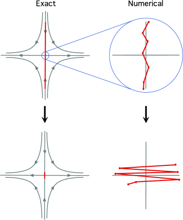
Figure 1.1. Forward advection of a classic stable manifold (a repelling LCS over finite times). Inaccuracies in determining the initial location of the LCS lead to exponentially growing errors and accumulation along the unstable manifold even if numerical errors were fully absent in the advection.

A recent computational advance is offered by [3], showing how both repelling and attracting LCS can be simultaneously obtained either at $t_{1}$ or $t_{2}$ from a single numerical run. This approach renders an attracting LCS at a time $t\in[t_{1},t_{2}]$ as the advected image of the initial LCS position at time $t_{1}$. Similarly, the time-$t$ position of a repelling LCS can be obtained by backward-advecting its position from time $t_{2}$ to $t$. Both of these computations track attracting material surfaces, and hence are numerically robust. However, they involve the advection of LCS from two different initial times, and hence are necessarily preceded by two separate numerical advections of a dense enough grid of initial conditions. Altogether, therefore, the computational cost of constructing both repelling and attracting LCS at arbitrary times $t\in[t_{1},t_{2}]$ has remained relatively high.

Here we propose a new computational strategy for two-dimensional incompressible flows. Our strategy builds on results from [3], [9] and [13, 11], enabling the reconstruction of all hyperbolic LCS for arbitrary times $t\in[t_{1},t_{2}]$ in a numerically robust fashion. This approach involves a single integration of trajectories from a full numerical grid, followed by the advection of select attracting material segments from local extrema of the singular value field of the flow gradient. This procedure yields substantial savings in computational time, as well as increased numerical accuracy in LCS detection and tracking. We demonstrate these advantages on a simple analytical flow example and on a direct numerical simulation of two-dimensional turbulence.

This paper is organized as follows. In Section 2, we fix our notation and recall relevant findings from [9] on the singular value decomposition of the linearized flow map. In Section 3 we present our attraction-based approach to hyperbolic LCS in the context of the recent geodesic theory of LCS [6, 2, 1]. In Section 4, we provide a proof of concept in the autonomous Duffing oscillator and compare our approach to previous ones in a simulation of two-dimensional turbulence, before concluding in Section 5.

2. Set-up

Consider a smooth, two-dimensional vector field $v(x,t)$, defined over a finite interval $I\coloneqq\left[t_{1},t_{2}\right]$ and over spatial locations $x\in D\subset\mathbb{R}^{2}$. The trajectories generated by $v(x,t)$ satisfy the ordinary differential equation

(2.1) $$\dot{x}=v(x,t).$$

The $t_{1}$-based flow map is denoted by $F_{t_{1}}^{t_{2}}\colon x_{1}\mapsto x_{2}$, mapping initial values $x_{1}$ from time $t_{1}$ to their position at time $t_{2}$ along the corresponding solution of (2.1). We recall that the flow map is as smooth in $x_{1}$ as is $v$ in $x$.

At any $x_{1}\in D,$ the deformation gradient $DF_{t_{1}}^{t_{2}}(x_{1})$ is a matrix that admits a singular value decomposition (SVD) of the form

(2.2) $$DF_{t_{1}}^{t_{2}} =\Theta\Sigma\Xi^{\top}, \Theta=\begin{pmatrix}\theta_{2}&\theta_{1}\end{pmatrix},\Xi=\begin{pmatrix}\xi_{2}&\xi_{1}\end{pmatrix} \in O(2), \Sigma =\begin{pmatrix}\sigma_{2}^{\text{f}}&0\\ 0&\sigma_{1}^{\text{f}}\end{pmatrix},$$

with $\sigma_{2}^{\text{f}}\geq\sigma_{1}^{\text{f}}>0$ on the flow domain $D$. The numbers $\sigma_{2}^{\text{f}},\sigma_{1}^{\text{f}}$ are the singular values of $DF_{t_{1}}^{t_{2}}$; the columns of $\Xi$ (i.e., $\xi_{2}$ and $\xi_{1}$) are the right singular vectors of $DF_{t_{1}}^{t_{2}}$; the columns of $\Theta$ (i.e., $\theta_{2}$ and $\theta_{1}$) are the left singular vectors of $DF_{t_{1}}^{t_{2}}$. From (2.2), we see that

$$DF_{t_{1}}^{t_{2}}\left(x_{1}\right)\xi_{i}\left(x_{1}\right) =\sigma_{i}^{\text{f}}\left(x_{1}\right)\theta_{i}\left(x_{2}\right), x_{2} =F_{t_{1}}^{t_{2}}(x_{1}), i \in\left\{1,2\right\}.$$

We recall that the singular values $\sigma_{2}^{\text{f}}(x_{1})$ and $\sigma_{1}^{\text{f}}(x_{1})$ measure infinitesimal stretching and compression along the trajectory starting from $x_{1}$. Furthermore, the unit vectors $\xi_{2}\left(x_{1}\right)$ and $\xi_{1}\left(x_{1}\right)$ are the tangent vectors pointing to the directions of strongest stretching and compression under the linearized flow $DF_{t_{1}}^{t_{2}}(x_{1})$.

If the velocity field is incompressible, i.e., $\nabla_{x}\cdot v(x,t)\equiv 0$, then $\det\left(DF\right)=\sigma_{1}^{\text{f}}\sigma_{2}^{\text{f}}=1$, and consequently

(2.3) $$\sigma_{2}^{\text{f}} =1/\sigma_{1}^{\text{f}}.$$

As a result, local maxima of $\sigma_{2}^{\text{f}}$ (locally strongest-stretching points) coincide with local minima of $\sigma_{1}^{\text{f}}$ (locally strongest-compressing points). At any point $x_{1}\in D$, the average exponential rate of largest stretching over the time interval $\left[t_{1},t_{2}\right]$ of length $T=t_{2}-t_{1}$ is defined as

$$\Lambda^{\text{f}}\left(x_{1}\right)\coloneqq\frac{1}{T}\log\sigma_{2}^{\text{f}}\left(x_{1}\right),$$

which is referred to as the (forward) finite-time Lyapunov exponent (FTLE). In the incompressible case, Eq. (2.3) shows that the FTLE can equally well be considered as a measure of the strongest local compression at $x_{1}$.

For the backward flow from $t_{2}$ to $t_{1}$, the backward deformation gradient is given by

(2.4) $$DF_{t_{2}}^{t_{1}}(x_{2})=\left[DF_{t_{1}}^{t_{2}}(x_{1})\right]^{-1}=\Xi\Sigma^{-1}\Theta^{\top},$$

with $\Sigma^{-1}=\begin{pmatrix}\sigma_{1}^{\text{b}}&0\\ 0&\sigma_{2}^{\text{b}}\end{pmatrix}=\begin{pmatrix}1/\sigma_{2}^{\text{f}}&0\\ 0&1/\sigma_{1}^{\text{f}}\end{pmatrix}$. The singular values of $DF_{t_{2}}^{t_{1}}$ are therefore given by

(2.5) $$\sigma_{2}^{\text{b}}(x_{2})=1/\sigma_{1}^{\text{f}}(x_{1}),\qquad\sigma_{1}^{\text{b}}(x_{2})=1/\sigma_{2}^{\text{f}}(x_{1}),\qquad x_{2}=F_{t_{1}}^{t_{2}}(x_{1}),$$

and the backward right singular vectors are given by $\theta_{1}$ and $\theta_{2}$, the strongest- and weakest-stretching directions at $x_{2}$ in backward time.

Eq. (2.3) shows that the maximal (minimal) singular value of the linearized flow map is equal to the maximal (minimal) singular value of the linearized inverse flow map. Thus, local maxima of $\sigma_{2}^{\text{f}}$ are mapped bijectively to local maxima of $\sigma_{2}^{\text{b}}$ by the flow map. We summarize the equivalences of local extrema of the forward and backward singular value fields as follows:

(2.6) $$\begin{array}[]{cccc}&x_{1}\text{ at }t_{1}&\xrightarrow{F_{t_{1}}^{t_{2}}}&x_{2}=F_{t_{1}}^{t_{2}}(x_{1})\text{ at }t_{2}\\ \\ &\sigma_{2}^{\text{f}}\text{--maximum}&\Longleftrightarrow&\sigma_{1}^{\text{b}}\text{--minimum}\\ \text{if incompressible}&\Updownarrow&&\Updownarrow\\ &\sigma_{1}^{\text{f}}\text{--minimum}&\Longleftrightarrow&\sigma_{2}^{\text{b}}\text{--maximum}.\end{array}$$

In terms of the backward FTLE field, we recover [7, Prop. 2] for the incompressible case:

$$\Lambda^{\text{b}}\left(x_{2}\right)=\frac{1}{T}\log\sigma_{2}^{\text{b}}\left(x_{2}\right)=\frac{1}{T}\log\left(\sigma_{1}^{\text{f}}\left(x_{1}\right)\right)^{-1}=\frac{1}{T}\log\sigma_{2}^{\text{f}}\left(x_{1}\right)=\Lambda^{\text{f}}\left(x_{1}\right).$$

In summary, as argued in [9], the SVD of $DF_{t_{1}}^{t_{2}}$ yields complete forward and backward stretch information from a uni-directional flow computation.

3. Forward and backward Geodesic Theory of Hyperbolic LCS

The following definition recalls the hyperbolic LCS candidates obtained from two-dimensional geodesic LCS theory.

Definition (Shrink and stretch lines, [2, 3]).

We call a smooth curve $\gamma$ a forward (or backward) shrink line, if it is pointwise tangent to the $\xi_{1}$ (or $\theta_{2}$) field. Similarly, we call $\gamma$ a forward (or backward) stretch line, if it is pointwise tangent to the $\xi_{2}$ (or $\theta_{1}$) field.

Shrink and stretch lines are solutions of a variational principle put forward in [1] for LCS. This principle stipulates as a necessary condition that the time $t_{1}$ positions of hyperbolic LCS must be stationary curves of the averaged Lagrangian shear [1]. This variational principle leads to the result that time $t_{1}$ positions of hyperbolic LCS are necessarily null-geodesics of an appropriate Lorentzian metric associated with the deformation field [1]. This prompts us to refer to the underlying approach as geodesic LCS theory.

Away from points where $\sigma_{2}^{\text{f}}=\sigma_{1}^{\text{f}}$ at $t=t_{1}$ and $\sigma_{2}^{\text{b}}=\sigma_{1}^{\text{b}}$ at $t=t_{2}$, both the initial and the final flow configuration is foliated continuously by mutually orthogonal forward and backward shrink and stretch lines. As discussed in [3, 9], the following equivalence relations hold:

(3.1) $$\begin{array}[]{ccc}\text{at }t_{1}&\xrightarrow{F_{t_{1}}^{t_{2}}}&\text{at }t_{2}\\ \text{}\\ \text{forward shrink line}&\Longleftrightarrow&\text{backward stretch line}\\ \perp&&\perp\\ \text{forward stretch line}&\Longleftrightarrow&\text{backward shrink line}.\end{array}$$

The forward shrink and stretch lines provide candidate curves for the positions of repelling and attracting LCS at time $t_{1}$. To find the positions of actual hyperbolic LCS as centerpieces of observed tracer deformation, we seek members of these two line families that evolve into locally most attracting or repelling material lines over the time interval $[t_{1},t_{2}].$

To this end, we follow [13, 11] to require a sufficient condition that hyperbolic LCS must satisfy. Specifically, the time $t_{1}$ positions of forward repelling LCS are shrink lines that intersect local maxima of $\sigma_{2}^{\text{f}}$; the time $t_{1}$ positions of forward attracting LCS are stretch lines that intersect local minima of $\sigma_{1}^{\text{f}}$. The time $t_{2}$ positions of backward-repelling and backward-attracting LCS are defined analogously using the backward singular-value fields $\sigma_{2}^{\text{b}}$ and $\sigma_{1}^{\text{b}}$. By the equivalences detailed above, forward-attracting LCS, as evolving material lines, coincide with backward repelling LCS. Similarly, forward-repelling LCS, as evolving material lines, coincide with backward-attracting LCS.

If the vector field $v(x,t)$ is incompressible, then the relation (2.3) forces local maxima of $\sigma_{2}^{\text{f}}$ to coincide with local minima of $\sigma_{1}^{\text{f}}$. As a consequence, both forward-repelling and forward-attracting LCS intersect the maxima of $\sigma_{2}^{\text{f}}$ at time $t_{1}$. This fact will simplify our upcoming computational algorithm considerably for incompressible flows.

As noted earlier, reconstructing a full forward-attracting LCS as a material line involves advecting its time $t_{1}$ position under the flow map. This is a self-stabilizing numerical process, as it tracks an attracting surface. In contrast, reconstructing a forward-repelling LCS from its time $t_{1}$ position by flow advection is an unstable numerical process. Indeed, the smallest initial errors in identifying the LCS position are quickly amplified, as shown in Fig. 1.1.

Relations (2.6) and (3.1), however, allow us to compute the forward-repelling LCS equivalently as backward-attracting LCS. Specifically, forward-repelling LCS positions at a time $t\in[t_{1},t_{2}]$ can be equivalently obtained from advection under the backward flow map $F_{t_{2}}^{t}.$ The curves to be advected under $F_{t_{2}}^{t}$ are just the backward stretch lines running through local minima of $\sigma_{1}^{\text{b}}$. By (2.5), however, local minima of $\sigma_{1}^{\text{b}}$ are just the images of local maxima of $\sigma_{2}^{\text{f}}$ under the flow map $F_{t_{1}}^{t_{2}}$.

The computation of stretch lines still involves the integration of direction fields, for which orientation issues have to be resolved (see [14, 2]). A new feature we introduce here is to advect short line segments (tangents) as opposed to whole stretch lines running through the appropriate extrema of the singular value fields. This idea exploits the tangentially stretching and normally attracting nature of stretch lines, saves on computational cost, and produces highly accurate results, as we demonstrate later. We summarize our attraction-based LCS construction in Fig. 3.1 for the case of incompressible flows. For compressible flows, forward-attracting LCS at time $t_{1}$ are still constructed from local minima of $\sigma_{1}^{\text{f}}$, but backward-attracting LCS at $t_{2}$ are constructed from advected local maxima of $\sigma_{2}^{\text{f}}$, which generally differ from advected local minima of $\sigma_{1}^{\text{f}}$.

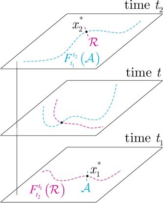
Figure 3.1. Illustration of the attraction-based LCS extraction for an incompressible flow at an arbitrary time $t\in[t_{1},t_{2}].$ Here $\mathcal{A}$ denotes a short vector parallel to $\xi_{2}$ at a local maximum $x_{1}^{*}$ of the $\sigma_{2}^{\text{f}}(x)$ field . Similarly, $\mathcal{R}$ denotes a short vector parallel to $\theta_{1}$ at the point $x_{2}^{*}=F_{t_{1}}^{t_{2}}(x_{1}^{*})$. Recall that both forward-repelling and forward-attracting LCS intersect the maxima of $\sigma_{2}^{\text{f}}$ at time $t_{1}$ in case of incompressibility.

Numerical implementation

Here we summarize the computational steps resulting from our previous considerations, assuming a forward-time advection of the chosen numerical grid.

1. Compute flow map and its linearization: We solve the ODE (2.1) from a sufficiently dense grid of initial conditions to obtain a discrete approximation to the flow map $F_{t_{1}}^{t_{2}}$. We also obtain a numerical approximation to the linearized flow map $DF_{t_{1}}^{t_{2}}$ at the grid points by one of four methods: (i) solving the equation of variations associated with (2.1), (ii) finite-differencing $F_{t_{1}}^{t_{2}}$ along the grid, (iii) finite-differencing on a smaller auxiliary grid [2], (iv) via convolution with Gaussian kernels [12].

2. Compute singular values: We compute the singular-value decomposition of the deformation gradient tensor field $DF_{t_{1}}^{t_{2}}$. This yields the singular values $\sigma_{i}^{\text{f }}$ as well as the right- and left-singular vector fields $\xi_{i}$ and $\theta_{i}$, respectively. The singular values $\sigma_{i}^{\text{b }}$ are obtained directly from the relation (2.5).

3. Select seeding points for LCS: We need to identify points of strongest attraction, i.e. local minima of $\sigma_{1}^{\text{f}}$ at the initial time and local minima of $\sigma_{1}^{\text{b}}$ at the final time. While the first are identified directly, the latter are advected images of local maxima of $\sigma_{2}^{\text{f}}$ under the flow map $F_{t_{1}}^{t_{2}}$. In the incompressible case, the points of strongest attraction coincide with local maxima of $\sigma_{2}^{\text{f}}$ and their advected images under $F_{t_{1}}^{t_{2}}$, respectively. As in [11], we start by sorting all local maxima in ascending order by the values of $\sigma_{1}^{\text{f}}$ or descending order by the values of $\sigma_{2}^{\text{f}}$. We then pick the first point $p_{1}$ in the ordered list and discard all local extrema in a small neighborhood of $p_{1}$. From the remaining points on the list, we pick the first point $p_{2}$ and discard extrema in a small neighborhood of $p_{2}$, and so on. This procedure filters out local extrema in noisy singular value fields.

4. Compute hyperbolic LCS: For any time $t\in[t_{1},t_{2}]$ of interest, we use the flow map $F_{t_{1}}^{t}$ to advect short line segments tangent to $\xi_{2}(p_{i})$ at the points $p_{i}$ identified in the previous step. The resulting set of curves form the time $t$ positions of attracting LCS. In the incompressible case, we use the flow map $F_{t_{2}}^{t}$ to advect short line segments tangent to $\theta_{1}(F_{t_{2}}^{t}(p_{i}))$ at the points $F_{t_{1}}^{t_{2}}(p_{i})$. Recall that the characteristic stretching directions for the backward flow are obtained from the forward time computation in step (2) due to Eq. (2.4). The resulting set of curves form the time $t$ positions of repelling LCS. For the advection of line segments, the use of an adaptive integration scheme may be necessary. This is to fill emerging large gaps between adjacent points due to stretching, and to mitigate the possibly high curvature in the tracked material curve (see, e.g., [10]).

4. Examples

4.1. Duffing oscillator

We first consider a rescaled version of the unforced, undamped Duffing oscillator with Hamiltonian

$$H(x,y)=\frac{1}{4}x^{4}-2x^{2}+\frac{1}{2}y^{2}.$$

This example has already been used to illustrate shrink and stretch line context by [3] locally around the origin, showing the convergence of forward- and backward maximal stretch directions to the unstable and stable subspaces, respectively. In our present computations, we use the times $t_{1}=0$ and $t_{2}=T=2.5$.

In Fig. 4.1, we compare the results from the earlier numerical LCS detection scheme used in [6] to our approach described in Section 3. While the left plot shows all structures to highlight the homoclinic loop, the middle plot shows that the shrink line deviates from the loop visibly at the first turn. In contrast, the backward-advected line segment stays close to the loop. The right plot shows that at the origin, both the shrink line and the advected stretch line indicate consistently the direction of strongest attraction.

Fig. 4.2 gives further quantitative evidence that the backward-advected backward stretch line gives a better approximation to the actual repelling LCS position at time $t_{1}$ than the direct computation of this LCS position from forward shrink lines.

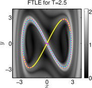
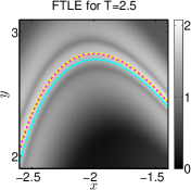
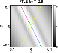
Figure 4.1. In the background, the FTLE field for integration time $T=2.5$ is shown. On top, we show the zero energy level $H=0$ (yellow), the shrink line (cyan), and a straight line aligned with $\theta_{1}(0)$ (short line segment not aligned with the homoclinic, magenta) at $t_{2}=2.5$ together with its image at $t_{1}=0$ (magenta). The left figure shows that all structures highlight the homoclinic loop with reasonable accuracy. The magnification in the middle shows, however, a significant deviation of the shrink line from the stable manifold. At the same time, the backward-advected straight line segment approximates the stable manifold perfectly. The right plot shows both the shrink line and the image of the backward stretch line segment to perform well near the origin.

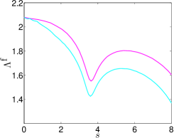
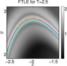
Figure 4.2. Left: Comparison of FTLE along the backward-advected backward stretch line (magenta) and the forward shrink line (cyan). Note that the advected stretch line has a uniformly higher repulsion rate and is therefore a better approximation to the repelling LCS. Right: Backward-advected particle blob of initial diameter $1.0$ (yellow), backward-advected stretch line (dashed magenta) and forward shrink line (cyan), showing that the advected stretch line is a better approximation to the backward attracting (i.e. repelling) LCS. (The numerical advection is performed by the Matlab routine ode45 with absolute and relative error tolerance of $10^{-8}$.)

Even in this simple example, therefore, the actual evolution of a shrink line and a backward-advected backward stretch line are noticeable different, although they should theoretically be identical. The root cause is numerical errors in the singular vector computation, as well as the limited ability of the discrete numerical grid to approximate a repelling LCS (local stable manifold) as a continuous curve. The error is initially invisible, but starts to accumulate rapidly during integration of the $\xi_{2}$ ($\theta_{1}$) field and advection.

4.2. Two-dimensional turbulence

As a second example, we consider the two-dimensional Navier–Stokes equations

$$\partial_{t}v+v\cdot\nabla v =-\nabla p+\nu\Delta v+f,$$

$$\nabla\cdot v =0,$$

$$v(\cdot,0) =v_{0},$$

where the unsteady velocity field $v(x,t)$ is defined on the two-dimensional domain $U=[0,2\pi]\times[0,2\pi]$ with doubly periodic boundary conditions. As in [3, 4], we use a standard pseudo-spectral method with 512 modes in each direction, and $2/3$ de-aliasing to solve the above Navier–Stokes equations with viscosity $\nu=10^{-5}$ on the time interval $\left[0,100\right]$. The flow integration is then carried out over the interval $t\in[50,100]$, in which the turbulent flow has fully developed, by a fourth-order Runge–Kutta method with variable step-size. The initial condition $v_{0}$ is the instantaneous velocity field of a decaying turbulent flow. The external force $f$ is random in phase and band-limited, acting on the wave-numbers $3.5<k<4.5$.

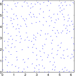
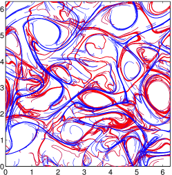
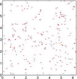
Figure 4.3. Attracting (blue) and repelling (red) LCS in a simulation of two-dimensional turbulence over the time interval $\left[50,100\right]$. Left: Initial line segments at $t_{1}=50$ for the attracting LCS. Middle: Hyperbolic LCS positions at $t=75$. Right: Initial line segments at $t_{2}=100$ for the repelling LCS.

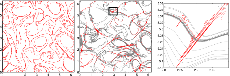
Figure 4.4. Left: shrink lines computed directly at $t_{1}=50$ as curves tangent to the $\xi_{1}(x)$ line field that intersect local maxima of $\sigma_{2}^{\text{f}}$. Middle: the same shrink lines (in red) advected to $t=75$ to highlight repelling LCS positions at that time. The gray curves are backward-advected stretch lines from $t_{2}=100$ that run through the time $t_{2}$ positions of trajectories starting from local maxima of $\sigma_{2}^{\text{f}}$ at time $t_{1}$. Right: a close-up view of the middle panel, clearly showing dramatic local inaccuracies from the forward calculation, resembling the effect shown in Fig. 1.1.

In Fig. 4.3(middle), we plot repelling (red) and attracting (blue) LCS at the middle time instance $t=75$. As described in Section 3, these LCS were launched as straight line segments of length $0.1$ from local $\sigma_{2}^{\text{f}}$–maxima and their flow images, which are $\sigma_{2}^{\text{b}}$–maxima, see Fig. 4.3(left) and (right). The filtering radius for local $\sigma_{2}^{\text{f}}$–maxima was set to $0.2$, yielding a reduction from $11,000$ to $229$ seeding points.

We plot forward shrink lines at the initial time $t_{1}=50$ in Fig. 4.4(left), and compare their forward-advected images (red) at the intermediate time $t=75$ with the backward advected stretch lines (gray), seeded at the corresponding points (see the middle panel of Fig. 4.4). Analytically, these curves should coincide. In some locations, they indeed agree well, but in other locations, the discrepancy is dramatic (see the close-up view in the right panel of Fig. 4.4). This is the consequence of the effect illustrated in Fig. 1.1, showing the clear advantage of our method over the forward-time tracking of a repelling LCS.

5. Conclusions

We have proposed a paradigm shift in the detection of hyperbolic Lagrangian Coherent Structures (LCS). Instead of detecting initial positions of LCS as curves of maximal forward repulsion, we seek them as backward-advected locations of maximal backward attraction. While these two approaches are theoretically equivalent, the latter approach (developed here) eliminates an inherent numerical instability of the former approach (used in prior work). We have demonstrated that our attraction-based approach leads to substantial improvements in accuracy and computational cost.

We have discussed our approach in the framework of the geodesic theory [6, 3, 1], because this theory allows for the explicit computation of hyperbolic LCS as parametrized curves. The proposed focus on attraction, however, automatically extends to potential future refinements in LCS computations.

The advection of identified hyperbolic LCS in the stable time direction is a simple idea, but relies heavily on the notion of a forward-time attracting LCS, which has been proposed only recently [3]. We have combined this notion with the SVD of the deformation gradient and with the seeding of straight line segments at points of locally strongest attraction to obtain a dynamically consistent and numerically robust approach to compute LCS. Extensions of these ideas to higher dimensions are possible and will be communicated elsewhere.

References

- [1] M. Farazmand, D. Blazevski, and G. Haller. Shearless transport barriers in unsteady two-dimensional flows and maps. Physica D, 278-279:44–57, 2014.
- [2] M. Farazmand and G. Haller. Computing Lagrangian coherent structures from their variational theory. Chaos, 22(1):013128, 2012.
- [3] M. Farazmand and G. Haller. Attracting and repelling Lagrangian coherent structures from a single computation. Chaos, 23(2):023101, 2013.
- [4] M. Farazmand and G. Haller. How coherent are the vortices of two-dimensional turbulence? 2014. submitted preprint.
- [5] G. Haller. Lagrangian Coherent Structures. Annual Review of Fluid Mechanics, 2015. to appear.
- [6] G. Haller and F. J. Beron-Vera. Geodesic theory of transport barriers in two-dimensional flows. Physica D, 241(20):1680–1702, 2012.
- [7] G. Haller and T. Sapsis. Lagrangian coherent structures and the smallest finite-time Lyapunov exponent. Chaos, 21(2):023115, 2011.
- [8] G. Haller and G. Yuan. Lagrangian coherent structures and mixing in two-dimensional turbulence. Physica D, 147(3-4):352–370, 2000.
- [9] D. Karrasch. Attracting Lagrangian Coherent Structures on Riemannian manifolds. 2013. submitted.
- [10] A. M. Mancho, D. Small, S. Wiggins, and K. Ide. Computation of stable and unstable manifolds of hyperbolic trajectories in two-dimensional, aperiodically time-dependent vector fields. Physica D, 182(3-4):188–222, 2003.
- [11] K. Onu, F. Huhn, and G. Haller. An Algorithmic Introduction to Lagrangian Coherent Structures. in preparation.
- [12] R. Peikert and F. Sadlo. Height Ridge Computation and Filtering for Visualization. In Visualization Symposium, 2008. PacificVIS ’08. IEEE Pacific, pages 119 –126, 2008.
- [13] B. Schindler, R. Peikert, R. Fuchs, and H. Theisel. Ridge Concepts for the Visualization of Lagrangian Coherent Structures. In R. Peikert, H. Hauser, H. Carr, and R. Fuchs, editors, Topological Methods in Data Analysis and Visualization II, Mathematics and Visualization, pages 221–235. Springer, 2012.
- [14] K.-F. Tchon, J. Dompierre, M.-G. Vallet, F. Guibault, and R. Camarero. Two-dimensional metric tensor visualization using pseudo-meshes. Engineering with Computers, 22(2):121–131, 2006.