Nonlocally-induced (quasirelativistic) bound states: Harmonic confinement and the finite well

Abstract

Nonlocal Hamiltonian-type operators, like e.g. fractional and quasirelativistic, seem to be instrumental for a conceptual broadening of current quantum paradigms. However physically relevant properties of related quantum systems have not yet received due (and scientifically undisputable) coverage in the literature. That extends to peculiarities of their nonlocally-induced dynamics and painfully lacking explicit insight into energy spectra under confining conditions. In the present paper we address Schrödinger-type eigenvalue problems for $H=T+V$, where a kinetic term $T=T_{m}$ is a quasirelativistic energy operator $T_{m}=\sqrt{-\hbar^{2}c^{2}\Delta+m^{2}c^{4}}-mc^{2}$ of mass $m\in(0,\infty)$ particle. A potential $V$ we assume to refer to the harmonic confinement or finite well of an arbitrary depth. We analyze spectral solutions of the pertinent nonlocal quantum systems with a focus on their $m$-dependence. Extremal mass $m$ regimes for eigenvalues and eigenfunctions of $H$ are investigated: (i) $m\ll 1$ spectral affinity (”closeness”) with the Cauchy-eigenvalue problem ($T_{m}\sim T_{0}=\hbar c|\nabla|$) and (ii) $m\gg 1$ spectral affinity with the nonrelativistic eigenvalue problem ($T_{m}\sim-\hbar^{2}\Delta/2m$). To this end we generalize to nonlocal operators an efficient computer-assisted method to solve Schrödinger eigenvalue problems, widely used in quantum physics and quantum chemistry. A resultant spectrum-generating algorithm allows to carry out all computations directly in the configuration space of the nonlocal quantum system. This allows for a proper assessment of the spatial nonlocality impact on simulation outcomes. Although the nonlocality of $H$ might seem to stay in conflict with various numerics-enforced cutoffs, this potentially serious obstacle is kept under control and effectively tamed.

I Motivation

The standard unitary quantum dynamics $\exp(-iHt/\hbar)$ and the Schrödinger semigroup-driven random motion $\exp(-tH/\hbar)$ are examples of dual evolution scenarios, connected by means of an analytic continuation in time (here e.g. $it\rightarrow t$ for times $t\geq 0$). Both types of motion share in common a local Hamiltonian operator $H$. Its spectral resolution is known to determine simultaneously transition amplitudes of the Schrödinger picture quantum motion in $L^{2}(R^{n})$ and transition probability densities of a space-time homogeneous diffusion process in $R^{n}$, with $n\geq 1$. The considered Hamiltonians have the form $H=T+V$, where the energy operator $T$ derives from the Laplacian and $V$ is a locally defined confining potential.

Within the general theory of so-called infinitely divisible probability laws the familiar Laplacian (probabilistically interpreted as the Wiener noise or Brownian motion generator) is merely one isolated member of a rich family of non-Gaussian Lévy noise generators. They stem from the fundamental Lévy-Khintchine formula, provided we restrict considerations to symmetric (typically heavy-tailed) probability distributions of spatial jumps and resultant jump-type Markov processes, c.f. GS .

The emergent Lévy generators are manifestly nonlocal (pseudo-differential) operators that give rise to Lévy-Schrödinger semigroups and to nonlocally-induced random dynamics. The dual (Euclidean) image of the latter, comprises unitary dynamics scenarios that exemplify an inherently nonlocal quantum behavior.

The canonical quantization concept we introduce indirectly, by choosing the Hilbert space $L^{2}(R^{n})$ as an arena for investigations. From the start we have the Fourier transformation realized as a unitary operation in this space, a pre-quantum version of uncertainty relations (due to G. H. Hardy, c.f. GS ) and standard (i.e. pedestrian nonrelativistic quantum mechanics) notions of position and momentum operators as a consequence. Our further discussion will be restricted to one spatial dimension ($1D$), which is not a must but a pragmatic simplification of otherwise potentially clumsy reasoning, see however Ref. GS for less restrictive considerations.

The Lévy-Khintchine formula, while tailored for our purposes, derives from a Fourier transform of a symmetric probability density function. A variety of such probability laws for random noise is classified by means of a characteristic function which, while restricted to $1D$, is an exponent $\eta(p)$ of the $(2\pi)^{1/2}$-multiplied Fourier transform of that probability density function (pdf), $\int dx\,\rho(x)\exp(\pm ipx)=\exp[\eta(p)]$. The canonical quantization recipe $p\rightarrow\hat{p}=-i\nabla$ (natural units $\hbar=1=c$ being implicit), while executed upon the characteristic function, induces Lévy-Schrödinger semigroups $\exp[t\eta(\hat{p})]$ that drive random jump-type processes.

As mentioned before, dual partners of semigroup operators are unitary evolution operators $\exp[it\eta(\hat{p})]$ which here by set a broadened (e.g. going beyond the local paradigm) quantum mechanical context.

By redefining the characteristic exponent as $\eta(p)=-F(p)$ and subsequently $F(\hat{p})=T$, we can classify probability laws of interest and next the emergent energy operators, in a bit more physical vein. Those are: (i) symmetric stable laws that correspond to $F^{\mu}(p)=|p|^{\mu}$, with $\mu\in(0,2)$ and give rise to so-called fractional energy operators $T^{\mu}=(-\Delta)^{\mu/2}\doteq|\nabla|^{\mu}$, (ii) quasirelativistic probability law inferred from $F_{m}(p)=\sqrt{p^{2}+m^{2}}-m$, $m>0$ which is a rescaled version (no $c$) of a classical relativistic Hamiltonian $\sqrt{m^{2}c^{4}+c^{2}p^{2}}-mc^{2}$. Accordingly, in natural units $\hbar=c=1$, $T_{m}=\sqrt{-\Delta+m^{2}}-m$ stands for the quasirelativistic energy operator. We note that $F^{1}(p)=|p|$ determines the Cauchy probability law and gives rise to Cauchy operator, here denoted $T^{1}=(-\Delta)^{1/2}\doteq|\nabla|$. Clearly $T^{1}=T_{0}$.

We are interested in solving Schrödinger-type eigenvalue problems for Hamiltonians of the form $H=T+V$, where $T$ may be a nonlocal energy operator, while $V$ is a locally defined confining potential. The latter we specify to be either harmonic or refer to a finite well of arbitrary depth. Under these confining conditions, the Cauchy oscillator and Cauchy (in)finite well were investigated Ref. GZ .

In the present paper we shall consider quasirelativistic Hamiltonians $T_{m}$ as energy operators of interest and subsequently compute a number of their nonlocally-induced bound states in harmonic and finite well regimes. Recently reported approximate quasirelativistic infinite well spectral solution ($m>0$ ”particle in the box” problem KKM ), together with that for the Cauchy infinite well K ; GZ and known spectral solution for the Cauchy (massless) harmonic oscillator SG ; LM , provide verification tools for our quasirelativistic spectral results, once we turn over to the $m\ll 1$ regime of the corresponding quasirelativistic spectral problems. In the $m\gg 1$ extreme a direct comparison will prove possible with the standard nonrelativistic spectral data. We shall give more explicit meaning to those ”small” versus ”large” mass regimes in below.

If an analytic solution of the ”normal” Laplacian-based Schrödinger eigenvalue problem is not in the reach, a recourse to the imaginary time propagation technique (to evolve the system in ”imaginary time”, to employ ”diffusion algorithms”) is a standard routine BBC -Chin . There exist a plethora of methods (mostly computer-assisted, on varied levels of sophistication and approximation finesse) to address the spectral solution of local 1D-3D Schrödinger operators in various areas of quantum physics and quantum chemistry. Special emphasis is paid there to low-lying bound states, were ”low-lying” actually means that even few hundred of them are computable.

The major goal of the present paper is to generalize the above mentioned ”diffusion algorithms” so that the resultant ”jump-type algorithms” would provide reliable high accuracy approximations to true spectral solutions for the quasirelativistic Hamiltonian in the wide mass parameter range $m\in(0,\infty)$. All computations are carried out in configuration space, thus deliberately avoiding a customary usage of Fourier transforms which blur an inherent spatial nonlocality of the problem. We keep under control the balance between the nonlocality impact and various (lower and upper) bounds upon the integration volume and the space-time intervals partitioning finesse, that are unavoidable in numerical procedures.

We are very detailed about the (bottom) part of the spectrum, somewhat disregarding higher eigenvalues (except for a number of approximate formulas). Some steps (like e.g. the choice of the Gram-Schmidt orhonormalization procedure) of the spectrum generating algorithm were tailored specifically to this end.

Compared with nonlocal spectral problems considered in the literature so far, even though our computations are carried out for rescaled versions of original models (thus devoid of explicit physical dimensions), we have kept intact the mass (for all models) and the well width and depth dependence. Moreover, albeit with dimensionless computation outcomes in hands, we can fully recover all physically relevant characteristics of considered models. An extended Appendix C gives details about how to eliminate and reintroduce physical (dimensional) constants, plus an assessment of involved length and energy scales.

II Spectrum-generating algorithm: An outline.

To deduce a spectral resolution (e.g. find eigenvalues and eigenfunctions) of a self-adjoint non-negative operator $H$, it is the ”imaginary time propagation” i.e. the semigroup dynamics $\exp(-tH)$ with $t\geq 0$ which is particularly well suited to this end, BBC ; AK . That, in view of obvious domain and convergence/regularization properties which are implicit in the Euclidean (or statistical like e.g. the partition function evaluation) framework.

Let us consider the eigenvalue problem for a self-adjoint operator $H$ of the form $H=T+V$, assuming that (at least a part of) the spectrum is strictly positive, discrete and non-degenerate $0<E_{1}<E_{2}<E_{3}<\ldots$ (the latter restriction may be lifted, since it is known how to handle degenerate spectral problems, BBC ; AK ):

$$H\,\psi_{i}(x)=E_{i}\psi_{i}(x),\qquad i=1,2,\ldots,$$ (1)

where $T$ is not necessarily a local differential operator (like the negative of the Laplacian), but a nonlocal (pseudo-differential) operator.

In below we shall mostly refer to nonlocal operators $T$ defined through their action on suitable $L^{2}(R)$ functions in the domain of $H$:

$$T\,\psi(x)=p.v.\int[\psi(x)-\psi(x+z)]\,\nu(dz),$$ (2)

where $\nu(dz)=\nu(z)dz$ stands for so-called Lévy measure and generically the $1D$ integral in Eq. (2) is interpreted in terms of its Cauchy principal value: $p.v.\int f(z)\nu(dz)=\lim\limits_{\varepsilon\to 0}\int_{R\backslash(-\varepsilon,\varepsilon)}f(z)\nu(dz)$.

The choice of $\nu(z)=1/(\pi z^{2})$ identifies the Cauchy operator $T=(-\Delta)^{1/2}\doteq|\nabla|$, while that of

$$\nu_{m}(z)=\frac{m}{\pi}\frac{K_{1}(m|z|)}{|z|},$$ (3)

where $K_{1}$ is a modified Bessel function of the third kind, defines the quasirelativistic operator $T_{m}=\sqrt{-\Delta+m^{2}}-m$.

To define the spectrum-generating algorithm, we first need to introduce an approximation of the original semigroup dynamics $\exp(-tH)\psi$, of a suitable initial data vector $\psi$ for arbitrary $t>0$, by a composition of a large number of consecutive small time ”shifts”. To this end a recourse to Trotter-type formulas is necessary and the Strang splitting method produces a number of their approximations of varied orders.

In the present paper we shall focus on the simplest second order Strang approximation of the semigroup operator $\exp(-H\Delta t)$, where $H=T+V$ and $\Delta t\ll 1$, that has been widely used Auer in quantum physics and quantum chemistry contexts. The splitting identity

$$e^{-H\,\Delta t}\approx e^{-\frac{\Delta t}{2}V}e^{-\Delta t\,T}e^{-\frac{\Delta t}{2}V}$$ (4)

holds true up to terms of order $\mathcal{O}((\Delta t)^{3})$. Like in the standard quantum mechanical perturbation theory, the interpretation of the $\mathcal{O}(t^{3})$ term as ”sufficiently small” remains somewhat obscure, unless specified with reference to its action on functions in the domain of $H$.

A preferably long sequence of consecutive small time $\Delta t\doteq h$ ”shifts” of an initially given function $\psi(x,0)\rightarrow\psi(x,kh)$ with $k=1,2,...$, mimics the actual continuous evolution of $\psi(x,t)$ in the time interval $[0,kh]$. For sufficiently small times $\Delta t\doteq h$ we may take one more approximations step (keeping e.g. second and higher order terms of the Taylor series would improve an approximation accuracy):

$$e^{-hH}\approx e^{-\frac{h}{2}V}\left(1-hT\right)e^{-\frac{h}{2}V}\doteq\mathcal{S}(h).$$ (5)

The induced approximation error depends on the time step $h$ value. If $h$ is small, the error is small as well but the number of iterations towards first convergence symptoms is becoming large. Thus a proper balance between the two goals, e.g. the accuracy level and the optimal convergence performance, need to be established. (One more source of inaccuracies is rooted in the nonlocality of involved operators and spatial cutoffs needed to evaluate integrals. This issue we shall discuss later.)

We note that an optimal value of a ”small” time shift $\Delta t=h$, appears to be model-dependent. Subsequently, we shall refer to $h=0.001$.

An outline of the algorithm that is appropriate for a numerical implementation and ultimately is capable of generating approximate eigenvalues and eigenfunctions of $H$, reads as follows:

(i) We choose a finite number $n$ of trial state vectors (preferably linearly independent) $\{\Phi_{i}^{(0)},\,1\leq i\leq n\}$, where $n$ is correlated with an ultimate number of eigenvectors of $H$ to be obtained in the numerical procedure; at the moment we disregard an issue of their optimal (purpose-dependent) choice.

(ii) For all trial functions the time evolution beginning at $t=0$ and terminating at $t=h$, for all $1\leq i\leq n$ is mimicked by the time shift operator $S(h)$ of Eq. (5)

$$\Psi_{i}^{(1)}(x)=S(h)\Phi_{i}^{(0)}(x).$$ (6)

(iii) The obtained set of linearly independent vectors $\{\Psi_{i}^{(1)}\}$ should be made orthogonal (we shall use the familiar Gram-Schmidt procedure, although there are many others, AK ) and normalized. The outcome constitutes a new set of trial states $\{\Phi_{i}^{(1)},i=1,2,\ldots,n\}$.

(iv) Steps (ii) and (iii) are next repeated consecutively, giving rise to a temporally ordered sequence of $n$-element orthonormal sets $\{\Phi_{i}^{(k)}(x),i=1,2,\ldots,n\}$ and the resultant set of linearly independent vectors

$$\Psi_{i}^{(k+1)}(x)=S(h)\Phi_{i}^{(k)}(x),\qquad i=1,2,\ldots,n,$$

at time $t_{k+1}=(k+1)\cdot h$. We main abstain from its orthonormalization and stop the iteration procedure, if definite symptoms of convergence are detected. A discussion of operational convergence criterions can be found e.g. in Ref. Chin .

(v) The temporally ordered sequence of $\Phi_{i}^{(k)}(x)$, $k\geq 1$ for sufficiently large $k$ is expected to converge to an eigenvector of $S(h)$, according to:

$$S(h)\Phi_{i}^{(k)}(x)=e^{-hE_{i}^{(k)}}\Phi_{i}^{(k)}(x)\approx e^{-hE_{i}}\psi_{i}(x),$$ (7)

where $\psi_{i}$ actually stands for an eigenvector of $H$ corresponding to the eigenvalue $E_{i}$. Here:

$$E_{i}^{(k)}(h)=-\frac{1}{h}\ln(\mathcal{E}_{i}^{k}(h)),$$ (8)

where

$$\mathcal{E}_{i}^{k}(h)=<\Phi_{i}^{(k)}|\Psi_{i}^{(k+1)}>=<\Phi_{i}^{(k)}|S(h)\Phi_{i}^{(k)}>,$$

is an expectation value of $S(h)$ in the $i$-th state $\Phi_{i}^{(k)}$.

It is the evaluation of $\Phi_{i}^{(k)}(x)$ and $E_{i}^{(k)}(h)$ that is amenable to computing routines and yields approximate eigenfunctions and eigenvalues of $H$. The degree of approximation accuracy is set by the terminal time value $t_{k}=kh$, at which earlier detected symptoms of convergence ultimately stabilize, so that the iteration (i)-(v) can be stopped.

Remark: Even in the high-fidelity computation regime (c.f. BBC -Chin ), we never arrive at exact eigenfunctions and eigenvalues, but at their more or less accurate approximations. Therefore we should properly identify and keep under control various computation inaccuracies, coming from different sources. A model-independent inaccuracy source lies in our choice $h=0.001$ of the ”elementary” time shift (actually, a partition unit for any time interval). It is a matter of a preparatory numerical ”experimentation” whether the $h$ choice needs to be finer or not (e.g. $10^{-4}$ or $10^{-5}$). The price paid is a significant computing time increase. Besides a low (second) order of the Strang splitting of the semigroup operator, other inaccuracies of numerical procedures are model-dependent and come from the spatial nonlocality of involved operators (2) that stays in conflict with cutoffs needed to evaluate the integrals. In $1D$, we need a priori to declare that $x\in[-a,a]$, $a>0$. How wide the spatial interval should be to yield reliable simulation outcomes, especially for eigenvalues (the eigenfunction computation is less sensitive to the choice of $a\geq 50$), is again a matter of a numerical experimentation. We set the spatial partition unit $\Delta x=0.001$. In view of pre-selected $[-a,a]$ integration boundary limits, irrespective of the initial data choice $\{\Phi_{i}^{(0)}\in L^{2}(R)\}$, the simulation outcome is automatically placed in $L^{2}([-a,a])$. For the quasirelativistic and Cauchy oscillators, true eigenfunctions extend over the whole real line. Therefore, a computer-assisted spectral solution effectively provides an approximation of true eigenfunctions by suitable approximating functions with a support in $[-a,a]$. Clearly, the value of $a$ cannot be too small. We have found a threshold value $a=50$ to be an optimal choice (accuracy versus computation time, see also GZ ). This pertains as well to the computationally ”dangerous” regime of small masses $m\in(0,1]$. Then e.g. the eigenfunctions falloff at infinity becomes close to inverse polynomial ($\leq 1/|x|^{4}$ in the Cauchy case). We note that one can improve an accuracy of computations in the small mass regime. To this end a partitioning of the integration interval should be make finer than the adopted one $\Delta x=0.001$ (like e.g. $0.0001$).

III Quasirelativistic harmonic oscillator.

In Ref. GZ we have tested a predictive power of the just outlined computer-assisted method of solution of the Schrödinger-type spectral problem for a non-local operator $H$, through a comparison with an available analytic solution of the $1D$ Cauchy oscillator problem SG ; LM . That was subsequently followed by an analysis of to the Cauchy finite well problem and an in-depth analysis of various inadequacies of hitherto proposed (would-be) spectral solutions of the Cauchy infinite well problem.

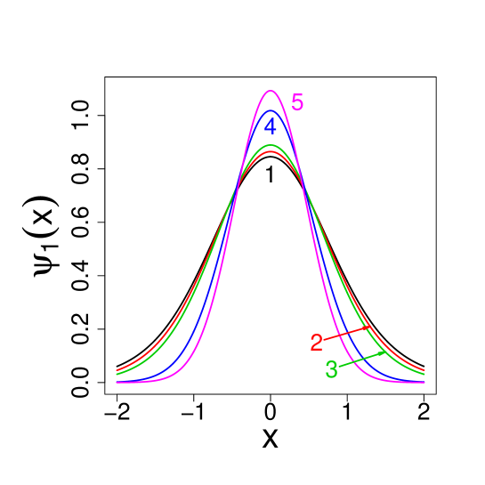
Figure 1: Quasirelativistic oscillator ground state (n=1) is depicted for masses $m=0.01,\,0.5,\,1,\,5,\,10$, labeled respectively by $1,\,2,\,3,\,4,\,5$. A clear distinction is seen between tentative ”small” mass $m\leq 1$ and ”large” mass $m\geq 5$ regimes. The $m=0.01$ curve is fapp identical with the ground state of the Cauchy oscillator, whose decay is known to be inverse polynomial $\sim C/x^{4}$, SG ; GZ .

In contrast to the $m=0$ regime, spectral data for $m>0$ quasirelativistic harmonic oscillator (in $1D$-$3D$) are scarce and not available in a closed analytic form. That enforces a computer-assisted approach, where the $m$-dependence needs to be optimally accounted for, in the whole range $m\in(0,\infty)$. As far as we know the literature on the subject, neither the quasirelativistic oscillator nor the quasirelativistic finite well problems were ever addressed on a similar to BBC -Chin level of computational accuracy. In fact, we can safely conjecture that the spectral solution in $1D$ and $2D$ is non-existent in the literature, while the available $3D$ data are rather limited, Hall ; Lucha ; Remb .

We are aware of a long-term research on quasirelativistic bound states (primarily in $3D$) for various confining potentials, including that of the harmonic oscillator Hall ; Lucha and the radial version of the $3D$ Cauchy oscillator Remb . Interestingly, the high-fidelity computer algorithm we advocate, has never been employed nor mentioned in those contexts. Moreover, we quite intentionally carry out spatial computations only, while computations of Refs. Lucha ; Remb were performed directly in the Fourier (momentum) representation, thus with no access to nonlocality-sensitive spatial diagnostics.

We are interested in spectral properties (eigenvalues and eigenfunctions) of the quasirelativistic harmonic oscillator $H=T_{m}+V=\sqrt{-\hbar^{2}c^{2}\Delta+m^{2}c^{4}}-mc^{2}+kx^{2}/2$. For computational simplicity and comparison with a number of related references, we shall work with a rescaled form of that Hamiltonian where, except for $m$, other dimensional parameters (or constants) are eliminated:

$$H=T_{m}+V=[\sqrt{-\Delta+m^{2}}-m]+x^{2}$$ (9)

The traditional coefficient $k/2$ in $V(x)=kx^{2}/2$ has been scaled away and the natural system of units $\hbar=1=c$ is implicit. How to eliminate or reintroduce dimensional constants and infer typical energy scales c.f. the Appendix.

The major preparatory guess, for an execution of the spectrum-generating algorithm, amounts to pre-selecting a suitable set (comprising one, two or more elements, see e.g. GZ for more detailed discussion) of linearly independent trial functions. There is a large freedom for that choice in $L^{2}(R)$ and in Ref. GZ the nonrelativistic harmonic oscillator basis (hermite functions) has been employed.

We are motivated by the fact that whatever this trial set is and whatever is its support ( $R$ or $[-1,1]\subset R$), in view of the integration volume restriction to $[-a,a]$, simulation outcomes are unavoidably placed in $L^{2}([-a,a])$ and $a=50$ is used throughout the paper. A computationally convenient choice of trial functions appears to be the standard nonrelativistic infinite well (”Laplacian in the interval”) eigenbasis for $[-1,1]\subset R$ which can be trivially extended to orthonormal $L^{2}(R)$ functions as follows:

$$\Phi_{n=2l-1}^{(0)}(x)=\left\{\begin{array}[]{ll}A\cos\left(\frac{n\pi x}{2}\right),&\hbox{$|x|<1$,}\\ 0,&\hbox{$|x|\geqslant 1$}\end{array}\right.\qquad\Phi_{n=2l}^{(0)}(x)=\left\{\begin{array}[]{ll}A\sin\left(\frac{n\pi x}{2}\right),&\hbox{$|x|<1$,}\\ 0,&\hbox{$|x|\geqslant 1$}\end{array}\right.\qquad l=1,2,\ldots$$

Here $A=\pm 1$.

Anticipating further discussion, we need to mention that numerical outcomes for simulated eigenvalues are $a$-sensitive in the small mass regime $m\ll 1$. Here small means e.g. $m=0.001,\,0.01$, albeit our subsequent discussion will validate $m=0.5$ or even $m=1$ to be ”sufficiently” small. However one needs to know that for $m=1$ the choice of $a=20$ gives practically the same outcomes as those for $a=50$ or $a=100,\,200$. (Our previous Cauchy oscillator discussion, GZ (see e.g. Figs. 1, 3 and 6), proved that appreciable (detectable) differences between computed lowest eigenvalues decrease, but still persist, while $a$ increases from $a=50$ through $a=100$, up to $a=500$.)

To the contrary, approximate low energy eigenfunctions can be satisfactorily reproduced within relatively small spatial interval like e.g. $[-3,3]$ or $[-5,5]$, beyond which these functions quickly decay. Their shape dependence on the integration bound $a\geq 50$ is residual and for all practical purposes (fapp) can be neglected.

Our numerical experimentation has shown definite stabilization/convergence symptoms after about $1.500-2000$ small $h$-time shifts (5)-(8), when computed eigenvalues (and shapes of eigenfunctions) effectively stop to change within the adopted error limits (that pertains to the eigenvalues evaluation up to four decimal digits).  We have found $k=2500$ to set an optimal terminal stabilization ”time” $t_{k}=k\,h$ at which our spectrum-generating algorithm can be stopped and data stored. To get more accurate data (up to the seven or eight decimal digits), the stabilization time should be increased (to $4.000$ or more $h$-time steps).

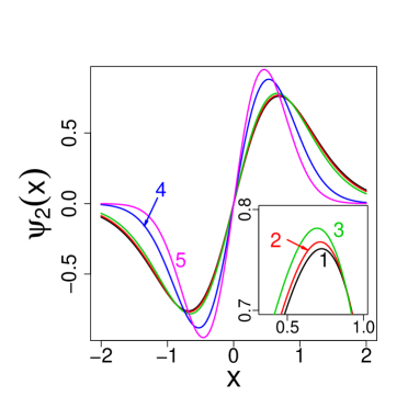
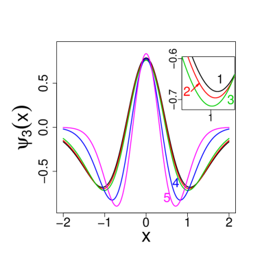
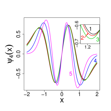
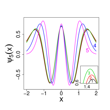
Figure 2: Quasirelativistic oscillator excited states ($n=2,3,4,5$) for $m=0.01,\,0.5,\,1,\,5,\,10$, labeled respectively by $1,2,3,4,5$, (parametr $a=50$). We note a clustering of curves in the ”low” mass regime. Insets depict an enlarged vicinity of the local minimum/maximum for curves $1,2,3$, identifiable by respective $(x,\psi(x))$ coordinates.

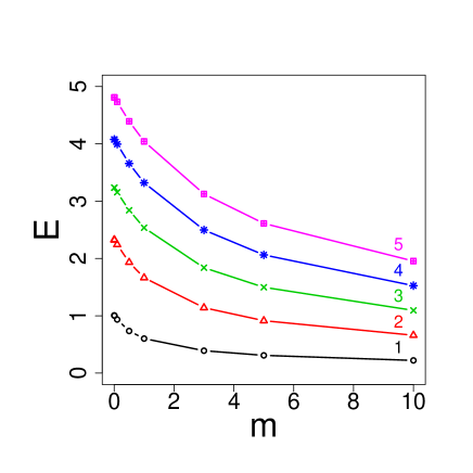
Figure 3: The $m$ dependence of the quasirelativistic oscillator eigenvalues with $n=1,\,2,\,3,\,4,\,5$. Employed $m>0$ values read: $0.001,\,0.01,\,0.1,\,0.5,\,1,\,3,\,5,\,10$. The $m=0$ energy values have been directly imported from the spectral solution of the Cauchy oscillator SG ; LM and cannot be graphically distinguished from those for $m=0.001$.

Since, for the quasirelativistic oscillator we are interested in the $m$-variability of eigenvalues and eigenfunctions of $H$, albeit unfortunately with no analytic formulas at hand, spectral data need to be computed for a number of explicit representative values of $m\in(0,\infty)$. We systematically refer to $m=0.01,\,0.5,\,1,\,3,\,5,\,10$, with brief appearances of $m=0.001$ and $m=20,\,50,\,100,\,200$, if a deeper insight into $m\ll 1$ or $m\gg 1$ regimes is necessary.

Let us add that for low-lying part of the spectrum, the decay properties of involved Bessel functions (3) get amplified by the mass parameter increase. Thus e.g. in case of $m=1$, for $|x|>20=a$, tails of Bessel functions are bounded from above by $10^{-21}$. For $m=5$, the integration bound $a=15$ or $a=20$ would give as good approximate results as that of $a=50$. Even for a relatively small mass $m=0.5$, the integration bound $a=40$ would suit pragmatically oriented scholars (e.g. accepting some degree of robustness in numerical calculations and the above mentioned fapp criterion).

In Fig. 1, the ground state function of $H=H_{m}=\sqrt{-\Delta+m^{2}}-m+x^{2}$ is depicted for mass parameter values $m=0.01,\,0.5,\,1$ (regarded as ”small”; notice a conspicuous clustering of pertinent curves) and $5,\,10$ (tentatively regarded as ”large”). For small $m$ values curves stay in a close vicinity of the Cauchy oscillator Hamiltonian (an ultrarelativistic $m=0$ limit of $H=H_{m}$). In case of $m=0.01$, within adopted graphical accuracy limits, the corresponding curve $1$ cannot be distinguished from the Cauchy oscillator ground state (c.f. Fig. 1 in Ref. GZ ).

Lowest excited states ($n=2,3,4,5$) are depicted in Fig. 2, for the same masses and $a$ as in Fig. 1. ”Small” $m$ curves $1,\,2,\,3\,$ cluster in a close vicinity of the Cauchy oscillator excited states. Those labeled by $1$ are fapp identical with their Cauchy relatives, see GZ .

As mentioned before, for the quasirelativistic oscilator, an accuracy with which the eigenvalues in the ”small” mass regime are computable, is $a$ sensitive. This issue we shall discuss in the next subsection.

Interestingly, beginning from $m\geq 1$ this $a$-sensitivity practically disappears, and our choice of $a=50$ is definitely oversized. Since the computing time drops down considerably for smaller values of $a$, we have positively tested an adequacy of $a<50$ integration bounds. Below we list first five numerically obtained eigenvalues, where for $m=1,3,5$ integrations we use $a=20$ , for $m=10,20$ we have found $a=10$ to be reliable, while for $m\geqslant 50$, the bound $a=5$ proved to be sufficient.

$V(x)=x^{2}$	m=1	$m=3$	$m=5$	$m=10$	$m=20$	$m=50$	$m=100$
$E_{1}$	0.6020	0.39043	0.30891	0.22112	0.15669	0.09936	0.06865
$E_{2}$	1.6638	1.1408	0.91436	0.65998	0.46904	0.29639	0.20562
$E_{3}$	2.5362	1.8385	1.4974	1.0939	0.77957	0.49125	0.34230
$E_{4}$	3.3210	2.4971	2.0620	1.5252	1.0886	0.68591	0.47874
$E_{5}$	4.0426	3.1253	2.6111	1.9540	1.3962	0.88136	0.61508

Table 1: Quasirelativistic oscillator: $m$-dependence of lowest five eigenvalues.

In Fig. 3 we display the $m$-dependence ($m\in[0.001,10]$) of first five computed quasirelativistic oscillator eigenvalues, where the small mass behavior clearly indicates a convergence towards the Cauchy oscillator spectrum. On the other hand, the large mass extreme (here reaching merely $m=10$) allows us to anticipate an affinity with the spectral solution of the nonrelativistic harmonic oscillator, to be analyzed subsequently.

In Table I, for reference, the $m$-dependence of five lowest eigenvalues is presented in the mass range $[1,100]$. The detailed analysis of the small mass regime we have relegated to the separate subsection.

III.1 $m\ll 1$ regime

III.1.1 Low mass eigenvalues

Small mass spectrum of the quasirelativistic oscillator, like that in the Cauchy case GZ , needs the integration interval bound $a$ not to be small. Actually, in the Cauchy case we have found $a=500$ to be reliable for lowest eigenvalues, while $a=50$ is predominantly employed in the present paper. Therefore it essential to investigate the $a$-dependence of computed eigenvalues for small mass values.

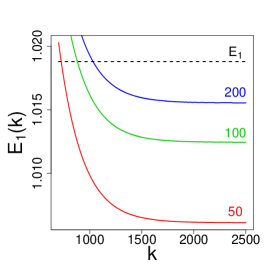
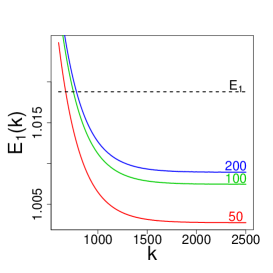
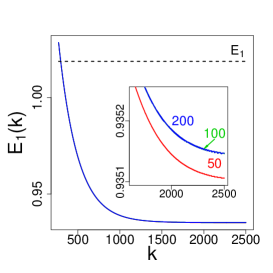
Figure 4: (k)-time evolution of $E_{1}^{(k)}(h)=-\frac{1}{h}\ln(\mathcal{E}_{1}^{k}(h))$ (8) and the stabilization symptoms in the computation of the ground state value: $m=0.001$ (left panel), $m=0.01$ (middle panel) and $m=0.1$ (right panel), for $a=50,\,100,\,200$. For reference we have depicted the energy level $E_{1}=1.018792$ which is set by the Cauchy oscillator bottom eigenvalue.

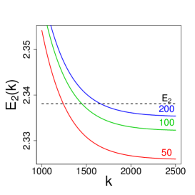
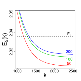
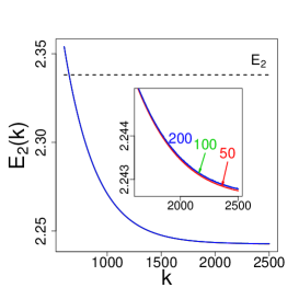
Figure 5: (k)-time evolution of $E_{2}^{(k)}(h)=-\frac{1}{h}\ln(\mathcal{E}_{2}^{k}(h))$ (8). Computation of the first excited eigenvalue for $m=0.001$ (left panel), $m=0.01$ (middle panel), $m=0.1$ (right panel), for $a=50,\,100,\,200$. $E_{2}=2.338107$ is the first excited Cauchy oscillator eigenvalue.

Our results are displayed In Figs. 4 and 5 for $m=0.001,0.01,0.1$, where a stabilization of the (k)-evolution (8) is clearly seen. A comparison of Fig. 4 with Fig.1 of Ref. GZ proves that the computed $m=0.001$ ground state eigenvalue for $a=200$ is extremely close to that obtained in the Cauchy case proper ($m=0$). With the growth of $m$ the bottom spectral value drops down. Moreover, the $a$-sensitivity quickly deteriorates. For $m=0.1$, $a=100$ and $a=200$ computation outcomes cannot be graphically distinguished in the scale employed. Albeit our primary bound $a=50$ still can be (residually) distinguished under an amplified resolution, as seen in the inset of the Fig. 4 right panel. In case of $m=1$ (not displayed), there would be no graphical differentiation at all between $a=50$, $a=100$ and $a=200$ computation outcomes.

An analogous stabilization behavior can be seen in the (k)-evolution (8) towards the first excited eigenvalue. The deterioration of $a$-sensitivity with the growth of $m$ is perfectly seen in middle and right panels (see the inset for details) of Fig. 5.

III.1.2 Spectral convergence to the Cauchy oscillator.

For reference, we first display five lowest eigenvalues of the Cauchy oscillator up to the sixth decimal digit, SG ; LM . Altogether $18$ lowest eigenvalues are listed in the Appendix. One should be aware that the finesse of explicit expressions for Cauchy oscillator eigenvalues varies in the literature and happens to extend to $14$ or more decimal digits.

m=0	$E_{1}$	$E_{2}$	$E_{3}$	$E_{4}$	$E_{5}$
SG ; LM	1.018792	2.338107	3.248197	4.087949	4.820099

Table 2: Cauchy oscillator lowest eigenvalues.

m=0.001	$E_{1}$	$E_{2}$	$E_{3}$	$E_{4}$	$E_{5}$
a=50	1.00612	2.32596	3.23723	4.07956	4.81614
a=100	1.01245	2.33229	3.24356	4.08590	4.82248
a=200	1.01555	2.33540	3.24667	4.08901	4.82560

Table 3: Quasirelativistic oscillator: $a$-dependence of lowest eigenvalues for $m=0.001$.

m=0.01	$E_{1}$	$E_{2}$	$E_{3}$	$E_{4}$	$E_{5}$
a=50	1.00275	2.32235	3.23367	4.07593	4.81255
a=100	1.00746	2.32707	3.23839	4.08066	4.81728
a=200	1.00893	2.32854	3.23987	4.08213	4.81876

Table 4: $a$-dependence for m=$0.01$.

m=0.1	$E_{1}$	$E_{2}$	$E_{3}$	$E_{4}$	$E_{5}$
a=50	0.935106	2.24274	3.15568	3.99499	4.73274
a=100	0.935146	2.24278	3.15573	3.99503	4.73278
a=200	0.935147	2.24278	3.15573	3.99503	4.73278

Table 5: $a$-dependence for $m=0.1$.

A comparison (Tables II to V) of quasirelativistic oscillator eigenvalues, in the descending mass order $m=0.1,\,0.01,\,0.001$, with those for the Cauchy oscillator clearly indicates the spectral convergence of the quasirelativistic oscillator to the Cauchy one as $m$ approaches $0$.

The clustering of ”small” mass curves in Figs. 1 and 3, corresponding to $m\in(0,1]$, gives support to the statement about the convergence of quasirelativistic spectral data to ultrarelativistic ones as $m$ drops down to $0$. In the Appendix we give additional analytic hints to this conclusion.

Accordingly, for small masses, the Cauchy oscillator provides a reliable spectral approximation of the quasirelativistic one in the whole spectral range (i.e. for arbitrarily large $n$). Thence, it is of interest to recall asymptotic (”large” $n$) regularities of Cauchy oscillator eigenvalues. Those may be adopted to approximate higher eigenvalues of the small mass quasirelativistic system. These regularities are quantified by means of handy analytic formulas SG ; LM . For odd labels $n$ we have:

$$E_{n=2k-1}\sim\left(\frac{3\pi}{2}\right)^{2/3}\left({n+\frac{3}{4}}\right)^{2/3}$$ (10)

while for even $n$ there holds

$$E_{n=2k}\sim\left(\frac{3\pi}{2}\right)^{2/3}\left({n+\frac{1}{4}}\right)^{2/3}$$ (11)

with $k=1,2,3,...$. Concerning an approximation accuracy, we must decide how large the label $n$ needs to be. The approximation finesse clearly depends on the a priori chosen robustness level and can be fine-tuned. In the present discussion we have found formulas (10) and (11) to give reliable approximations for relatively low labels $n\geq 6$, see the Appendix for detailed data.

III.2 $m\gg 1$ regime

The $m$-dependence of quasirelativistic oscillator eigenvalues for $m\in(0,10]$ depicted in Fig. 3, clearly indicates symptoms of $m\gg 1$ spectral regularities which need to be verified more convincingly. See e.g. the Appendix for analytic hints to this end. Clearly, mass values should be picked out well beyond the interval $(0,10]$. In Fig. 6 a sequence of eight consecutive (lowest) eigenvalues is depicted separately for each mass parameter $m=10,20,50,100$ separately. The dependence of $E_{n}(m)$ on $n$ indicates approximately equal spacings between consecutive energy levels.

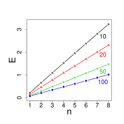
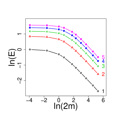
Figure 6: Quasirelativistic $m\gg 1$ regime. Left panel: eight consecutive eigenvalues $E_{n}(m)$, for masses $m=10,\,20,\,50,\,100$, build an approximate a straight line $E_{n}(m)={\frac{1}{\sqrt{2m}}}(2n-1)$, $n\geq 1$. The best result is obtained if fitting employs $m\geq 10$. Right panel: doubly logarithmic scale gives access to a wider mass range: $m=0.01,0.1,0.5,1,3,5,10,20,50,100$. Note that for $m>3.7$ i.e. $\ln(2m)>2$, straight line segments are mimicked by $\ln(E_{n}(m))=-\frac{1}{2}\ln(2m)+\ln(2n-1),\,n=1,2,3,4,5$, thus reproducing the nonrelativistic oscillator spectral pattern.

In the right panel of Fig. 6, the $E_{n}(m)$ data have been displayed (in a doubly logarithmic scale) against $2m$, for each fixed $n$ separately. That clearly identifies the $m$-dependence of the $n$-th eigenvalue ($n=1,...,8$) in a relatively wide mass range $m\in(0,100]$. The equal spacing conjecture receives even stronger support by fitting the numerically computed data to approximating straight lines (that in Fig. 4) of the form

$$E_{n}(m)=\frac{1}{\sqrt{2m}}(2n-1),\qquad n=1,2,\ldots\qquad m\gg 1,$$ (12)

or equivalently (that in Fig. 5)

$$\ln[E_{n}(m)]=-\frac{1}{2}\ln(2m)+\ln(2n-1),\qquad n=1,2,\ldots\qquad m\gg 1.$$ (13)

These formulas are approximately valid for sufficiently large $m$ and the $E_{n}(m)$ dependence on $n$ definitely appears to follow the nonrelativistic harmonic oscillator spectral pattern. In fact $E_{n}=\hbar\omega(n+{\frac{1}{2}}),\,n=0,1,...,$ where $\omega=\sqrt{k/m}$ derives from $H=-(\hbar^{2}/2m)\Delta+kx^{2}/2$. By scaling away $k$ (set formally $k=2$) and eliminating $\hbar=1$, we are left with $H=-(1/2m)\Delta+x^{2}$ whose spectral solution reads $E_{n}=\sqrt{\frac{2}{m}}\,(n+{\frac{1}{2}}),\,n\geq 0$. By relabeling that spectrum according to $n\rightarrow n-1$, where the former $n=0$ is replaced by the new $n=1$, we ultimately arrive at the formula $E_{n}=\sqrt{\frac{2}{m}}\,(n-{\frac{1}{2}})=\frac{1}{\sqrt{2m}}(2n-1),\,n\geq 1$, i.e. (12).

Concerning the fitting procedure, let us point out that in Fig. 6 we encounter functions of the form $\ln(E(m,n)=f[\ln(2m)]$. For mass values obeying $\ln(2m)>2$ (e.g. $m>3.7$) we can approximate the resultant curves by straight line segments of the form $\ln(E(m,n))=a\ln(2m)+b$. There, ”ideally” we should have $a=-1/2$ and $b=\ln(2n-1)$. Although an ”ideal” outcome is never the case, approximate values for $a$ and $b$ (retrieved form computed data) quite well fit to the nonrelativistic oscillator picture.

For concreteness we reproduce approximate values for $a$ and $b$ that determine straight line segment fits in Fig. 7, for first five eigenvalues. Error bounds were evaluated by means of the least square deviation method for computed spectral data. The fitting of straight lines has been actually started from $m=5$ for $n=1,2$ and $m=10$ for $n>2$.

$$n =1, (-0.501 \pm 0.005)\ln(2m)+(-0.012\pm 0.018), n=(0.994\pm 0.009).$$

$$n =2, (-0.497 \pm 0.006)\ln(2m)+(1.069\pm 0.021), n=(1.96\pm 0.03).$$

$$n =3, (-0.504 \pm 0.005)\ln(2m)+(1.606\pm 0.019), n=(2.99\pm 0.05).$$

$$n =4, (-0.503 \pm 0.005)\ln(2m)+(1.936\pm 0.019), n=(3.97\pm 0.07).$$

$$n =5, (-0.502 \pm 0.005)\ln(2m)+(2.18\pm 0.02), n=(4.92\pm 0.09).$$

Approximate values for the (right-hand-side) parameter $n$ were retrieved directly from the computed ”free” parameters $b=\ln(2n-1)$. We note that the parameter $a$ has fapp $a=-1/2$ value ( e.g. almost $-1/2$, within the error bounds). We recall that the data employed in Fig. 3 - 6 have been computed by means of the spectrum-generating algorithm which is not free of a number of error-accumulating factors (like. e.g the lowest order Strang approximation, the usage of Gram-Schmidt diagonalization procedure, finite bounds for the integration intervals etc.).

Nonetheless, an affinity with the nonrelativistic harmonic oscillator spectrum is clearly seen in the large mass regime. In our derivations, $m=10$ has been found to set a ”sufficiently large” threshold value such that for $m\geq 10$ the quasirelativistic harmonic oscillator spectrum effectively displays (approximates, becomes very close) the nonrelativistic oscillator spectral regularity $\Delta E=E_{i+1}-E_{i}\sim 1/\sqrt{2m}$, for all $i=1,2,...$.

IV Quasirelativistic finite well.

Let us consider the eigenvalue problem for $H=T+V$, where $T=T_{m}=\sqrt{-\Delta+m^{2}}-m$ is the quasirelativistic generator and

$$V(x)=\left\{\begin{array}[]{ll}0,&\hbox{$|x|<1$;}\\ V_{0},&\hbox{$|x|\geqslant 1$,}\end{array}\right.$$ (14)

with $V_{0}>0$. We use the natural system of units $\hbar=1=c$ from the start, see the Appendix for a description of involved scalings.

We shall discuss both shallow and very deep wells of the size $[-1,1]$. In the previous paper GZ we have demonstrated that a sufficiently deep finite Cauchy well is ”spectrally close” to the infinite Cauchy well. A number of eigenvalues and eigenfunctions has been computed for the low-lying part of the spectrum.

We mention that for sufficiently large $n$ the infinite quasirelativistic well ($[-b,b]$) eigenvalues can be approximated as follows, KKM (for a while we reintroduce dimensional constants, see also the Appendix):

$$E_{n}-mc^{2}=\left({\frac{n\pi}{2}}-{\frac{\pi}{8}}\right){\frac{\hbar c}{b}}+O\left({\frac{1}{n}}\right).$$ (15)

Interestingly, the right-hand-side of Eq. (15) has been proved in Ref. K to provide the large $n$ approximation of the $[-b,b]$ infinite Cauchy ($m=0$) well eigenvalues. Subsequently we shall restore the previously employed $b=1$ and $\hbar=1=c$ notation.

In the present Section we shall demonstrate that the finite quasirelativistic well, in the small mass regime, becomes ”spectrally close” to the finite Cauchy well (compare e.g. Cauchy versus quasirelativistic oscillator discussion of Section III). For another extreme of large masses, we shall demonstrate that the quasirelativistic well becomes ”spectrally close” to the familiar nonrelativistic finite well. Analytic arguments provided in the the Appendix give support to the conjecture that those extremal behaviors might be generic for a wider class of confining quasirelativistic problems.

Our numerical procedures are based on the spectrum-generating algorithm of Section II, including all mentioned there cutoff choices and the algorithm - related error accumulation reservations. We use $a=50$ for the integration interval bound. The set of trial functions is chosen to be the same as that in the discussion of Section III.

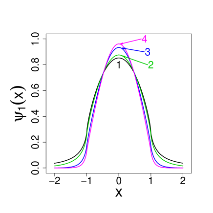
Figure 7: Quasirelativistic finite well ground state for $V_{0}=5$. Labels $1,2,3,4$ correspond to $m=0.01,1,5,10$, respectively.

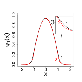
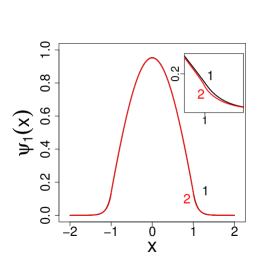
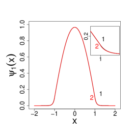
Figure 8: A comparison of ground states in case of $V_{0}=5$ for the nonrelativistic (label 1) and quasirelativistic well (label 2): $m=5$ (left panel), $m=10$ (middle panel), $m=20$ (right panel).

IV.1 Shallow well.

In a finite $1D$ (and $2D$) nonrelativistic well one normally expects at least one bound state to exist. The well known exception is the 3D case, when for too shallow wells (irrespective of their width) bound states may not exist at all. No general statements of that kind are known for nonlocal finite well problems.

We know the Cauchy well whose depth is set by $V_{0}=5$ has three bound states GZ . However, we have not explored before how low $V_{0}$ need to be to admit one bound state only. In the present paper this issue will be addressed on the level of a quasirelativistic finite well. An extension to finite Cauchy well will actually come out in the regime of small masses.

For concreteness and a direct comparison with results of Ref. GZ , let us begin our discussion from the finite $V_{0}=5$ quasirelativistic well. We have extended the stabilization time up to $5000$ small time steps. (Anticipating further discussion of the large $m$ regime when the Bessel functions become strongly localized, having very narrow peaks about their maxima and minima, a spatial partitioning has been made finer $\Delta x=0.001\rightarrow\Delta x=0.0005$.)

If $m$ drops down to a close vicinity of $0$, quasirelativistic eigenvalues and eigenfunctions appear to converge to those of the finite Cauchy well. To exemplify this observation on the level of eigenvalues let us provide explicit quasirelativistic ground state energy values in the $V_{0}=5$ well and set them against the respective $m=0$ value.

We have $E_{1}=0.9501$ for $m=0.01$, $0.9522$ for $m=0.001$ and $0.9538$ for the finite Cauchy well ($m=0$). Respective eigenfunctions are graphically indistinguishable in the adopted scale.

In Fig. 7 we depict quasirelativistic $V_{0}=5$ well eigenfunctions for graphically distinguishable cases of $m=0.01,\,1,\,5,\,10$. With the growth of $m$ the ground state maximum increases. Clearly, the eigenfunctions have tails extending beyond the well boundaries (e.g. the interval $[-1,1]$), but they decay rapidly with the growth of $|x|$. For large $m$ we detect a fairly close affinity with the standard (text-book) nonrelativistic finite well quantum problem (c.f. the Appendix for relevant data).

In accordance with the folk lore wisdom about the nonrelativistic finite well, in $1D$ at least one bound state is always in existence. However, the maximal number $N$ of bound states in the well of a fixed depth $V_{0}$ is correlated with the mass $m$ value (we bypass the well width impact, in view of our $[-1,1]$ choice). Indeed, the number of bound states $N\in\mathbb{N}$ is constrained by inequalities

$$\frac{\pi^{2}}{8V_{0}}(N-1)^{2}\leqslant m\leqslant\frac{\pi^{2}}{8V_{0}}N^{2}.$$ (16)

Physically more familiar inequalities in addition to dimensional constants explicitly involve the width parameter $b$ (the well interior is enclosed by $[-b,b]$). We display for reference the pertinent formula: $\pi^{2}\hbar^{2}(N-1)^{2}\leq 8mV_{0}b^{2}\leq\pi^{2}\hbar^{2}N^{2}$. Our considerations employ $b=1$ and $\hbar=c=1$. (In passing we note that in $1D$ and $2D$ well at least one bound state always exists. The bound state may not be granted to exist in $3D$ for too shallow wells.)

The above formula allows to deduce the number of bound states for a fixed well depth $V_{0}$ but different mass values. Thus e.g. for all $m\leq\pi^{2}/8V_{0}$ only one bound state is in existence. Accordingly the bound $m<1.23/V_{0}$ tells that for $V_{0}=5$ one bound state only is secured for masses $m<0.246$.

For comparison, maximal numbers of bound states of the $V_{0}=5$ well for various mass values are displayed in a compact Table VI. In the quasirelativistic case those were deduced by means of the spectrum-generating algorithm. In the nonrelativistic case (denoted ”standard”) these numbers were deduced from the formula (16). With the mass parameter increase, maximal numbers of bound states show a definite tendency to equalize for both local and nonlocal cases.

mass	quasirelativistic $N$	standard $N$
0.1	3	1
0.5	4	2
1	4	3
3	5	4
5	6	5
10	7	7

Table 6: $V_{0}=5$ well: maximal number $N$ of bound states for various masses in quasirelativistic and nonrelativistic cases.

With the growth of $m$ both eigenvalues and eigenfunctions for the nonlocal and local finite well models ”become close” to each other. To see this spectral affinity, let us compare respective eigenvalues in the well $V_{0}=5$, for various masses (for m=10, only $7$ eigenvalues are in existence):

mass	finite well	n=1	n=2	n=3	n=4	n=5	n=6	n=7	n=8
m=10	quasi	0.09951	0.39217	0.86271	1.48933	2.24605	3.10483	4.03221	-
	standard	0.10190	0.40679	0.91211	1.61267	2.49846	3.54752	4.68404	-
m=20	quasi	0.05312	0.21154	0.47264	0.83227	1.28482	1.82341	2.43999	3.12481
	standard	0.05379	0.21502	0.48318	0.85739	1.33616	1.91714	2.59636	3.36634
m=50	quasi	0.02227	0.08892	0.19968	0.35423	0.55213	0.79272	1.07522	1.39867
	standard	0.02261	0.09040	0.20334	0.36132	0.56421	0.81181	1.10385	1.43998
m=100	quasi	0.01126	0.04499	0.10113	0.17961	0.28037	0.40334	0.54842	0.71546
	standard	0.01159	0.04636	0.10431	0.18540	0.28964	0.41695	0.56733	0.74070

Table 7: Quasirelativistic (quasi) versus nonrelativistic (standard) $V_{0}=5$ well: $m$-dependence of eigenvalues

The resultant eigenvalues in case of $n>5$, even for large masses still differ by few percent. However we recall that our spectrum-generating algorithm accuracy has not been fined tuned to the available extent. A proper balance between cutoffs, partition units and the computations time was more important for us than the highest possible accuracy level (diminishing an accumulation of systematic errors) and that hampers computation results for $n>5$. C.f. also our comments concluding Sections II and III.B.

The eigenfunction computation is less sensitive to algorithm generated systematic errors. In Fig. 8 the ground state function of the quasirelativistic finite well is displayed (label 2) and compared with that for the nonrelativistic well (label 1) for masses $m=5,m=10,m=20$. We clearly see that $m=20$, albeit still too small, may be tentatively considered as the mass threshold above which the a concept of ”spectral closeness” of the quasirelativistic and nonrelativistic finite wells receives quantitative support.

A collection of excited eigenfunctions that are parametrized by the mass parametr $m$ is displayed in Fig. 9. The mass range $m=0.01,1,5,10$ is the same as in the ground state Fig. 7.

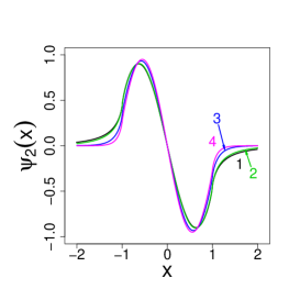
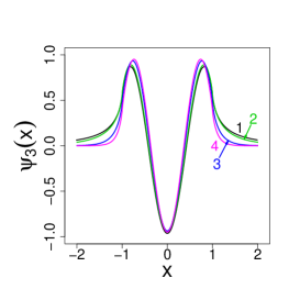
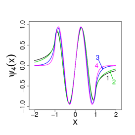
Figure 9: Second, third and fourth quasirelativistic $V_{0}=5$ well eigenfunctions. Masses $m=0.01,1,5,10$ are labeled respectively by $1,2,3,4$.

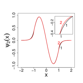
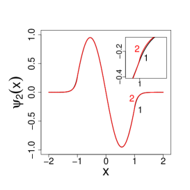
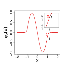
Figure 10: A comparison of the second eigenfunction in the $V_{0}=5$ well for nonrelativistic (label 1) and quasirelativistic (label 2) cases. Here, $m=5$ (left panel), $m=10$ (middle panel), $m=20$ (right panel).

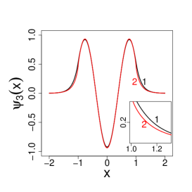
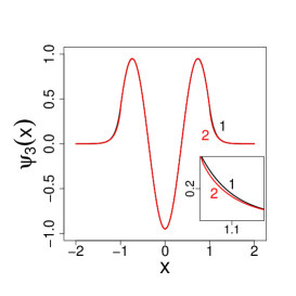
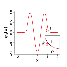
Figure 11: A comparison of the third eigenfunction in the $V_{0}=5$ well for nonrelativistic (label 1) and quasirelativistic (label 2) cases. Here, $m=5$ (left panel), $m=10$ (middle panel), $m=20$ (right panel).

In Figs. 10 and 11 we compare nonrelativistic and quasirelativistic finite ($V_{0}=5$) well eigenfunctions for $n=2,3$ ($n=4,5$ follow the same pattern) and masses $m=5,10,20$. We get there a convincing support to the previous tentative statement that $m=20$ is an optimal threshold value. For $m>20$, with a good fidelity, we can state that quasirelativistic and nonrelativistic finite wells are ”spectrally close”.

IV.2 Deep well versus infinite well.

Let us consider a relatively deep well $V_{0}=500$ (in Ref. GZ we have investigated the well as deep as $V_{0}=5000$). Like in the Cauchy finite well case, a quasirelativistic deep well is expected to stay in spectral affinity with its infinitely deep partner. That at least in relation to the low part of the spectrum.

For small values of the mass parameter $m$ convergence symptoms towards $m=0$ spectral solution are clearly seen in a sequence of ground state energies for the finite $V_{0}=500$ well: $E_{1}=1.1373$ for $m=0.01$, $1.1391$ for $m=0.001$, while $E_{1}=1.1408$ in the $m=0$ Cauchy case.

Eigenfunctions for small mass values are fapp graphically indistinguishable form their Cauchy relatives GZ . In Fig. 12 we have displayed quasirelativistic $V_{0}=500$ well ground state for masses $m=0.01,1,5,10$, where $m=5,10$ definitely stay beyond the ”smallness” range. For comparison the nonrelativistic infinite well ground state $\cos(\pi x/2)$ has been depicted. It is clear that all curves stay in a close vicinity of $\cos(\pi x/2)$, albeit upon enlargement they show subtle differences.

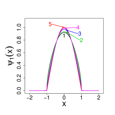
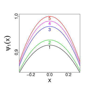
Figure 12: Quasirelativistic $V_{0}=500$ ground state. Labels $1,2,3,4$ refer to masses $m=0.01,1,5,10$. Label $5$ refers to the nonrelativistic infinite well ground state $\cos(\pi x/2)$. Right panel: an enlargment of the vicinity of the maxium.

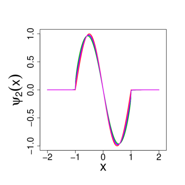
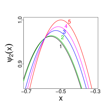
Figure 13: First excited state of the $V_{0}=500$ well. Labels $1,2,3,4$ refer to $m=0.01,1,5,10$, label 5 to the curve $-\sin(\pi x)$. Right panel: enlargement of the vicinity of maximum.

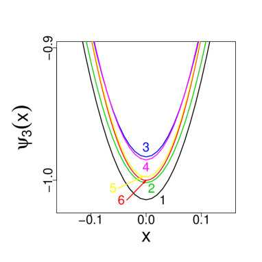
Figure 14: Third eigenfunction for $V_{0}=500$. Labels now refer to $m=0.01,1,5,10,50$, label 6 to the curve $-\cos(3\pi x/2)$. Right panel depicts an enlargement of the vicinity of the minimum.

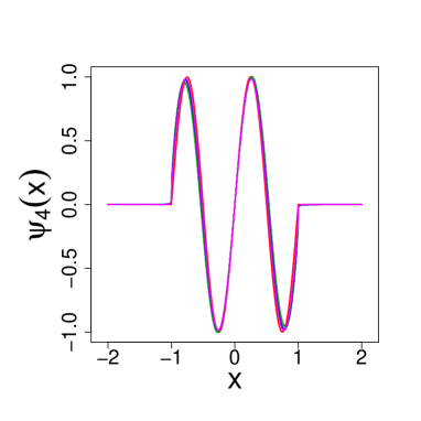
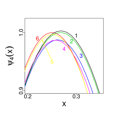
Figure 15: Fourth eigenfunctions for $V_{0}=500$. Labels $1,2,3,4,5$ refer to $m=0.01,1,5,10,50$, label 6 to the curve $\sin(2\pi x)$. Right panel: enlargement of the vicinity of the maximum.

We note that in case of $V_{0}=500$, for small $m$ respective ground states stay in a close vicinity of the infinite Cauchy well GZ . To the contrary, if $m$ is sufficiently large, respective ground states converge to $\cos(\pi x/2)$ which is a nonrelativistic ground state for an infinite well. The same pattern of behavior is detectable for excited states displayed in Figs. 13, 14 and 15.

The large $m$ regime locates excited states respectively in the vicinity of at $-\sin(\pi x)$ (Fig. 13), $-\cos(3\pi x/2)$ (Fig. 14) and $\sin(2\pi x)$ (Fig. 15). Due to the presence of $m=0.01$ curves we in fact have a transparent interpolation between the infinite Cauchy and nonrelativistic infinite well approximations of the deep quasirelativistic well. The convergence may not be uniform, see Fig. (15).

In the left panel of Fig. 16 the m-dependence of first five deep well ($V_{0}=500$) eigenvalues has been displayed. For a direct comparison the corresponding Cauchy well ($V_{0}=500,\,m=0$) eigenvalues were depicted as well. In the right panel the $n$-dependence of computed eigenvalues is displayed for masses $m=10,\,20,\,50,\,100$. The convergence towards Cauchy well data while $m$ drops down to $0$ is clearly seen. To the contrary, for large $m$ an approach towards the corresponding nonrelativistic well spectral data can be directly read out from the figures. We shall validate the latter statement by a more detailed data analysis.

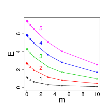
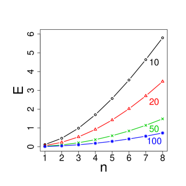
Figure 16: $V_{0}=500$ quasirelativistic well. Left panel: $E_{n}$ dependence on $m$, $n=1,2,3,4,5$. Right panel: computed eigenvalues are depicted against $n=1,2,3,4,5$. For each mass value ($m=10,20,50,100$) we depict a curve which is an optimal fit to the data.

On the basis of simulation data, we may fairly accurately deduce best fitting analytic forms for curves associated with masses $m=10,20,50,100$ (depicted in Fig. 16) and $m=200$ (not depicted so far. Since we expect a convergence (with the growth fo $m$) to nonrelativistic well spectral data, let us consider as a useful reference an approximate formula for the nonrelativistic deep well spectra GK ; BFV :

$$E_{n}^{V_{0}}\approx E_{n}^{\infty}\left(1-\frac{4}{\pi\sqrt{V_{0}}}\right)=\frac{\pi^{2}n^{2}}{8m}\left(1-\frac{4}{\pi\sqrt{V_{0}}}\right)$$ (17)

We note that $\frac{4}{\pi\sqrt{V_{0}}}<0.06$ for $V_{0}=500$.

For each mass parameter in the right panel of Fig. 16, the fitted fitting curve actually can be described by means of of an approximate analytic formula (derived directly from the data). For direct comparison, the ground state energy $E_{1}^{st}$ has been evaluated by means of a nonrelativistic formula (17). The spectral affinity of the quasirelativistic well with the nonrelativistic well for large mass values appears to be validated with no trace of doubt.

$$m =10, (0.1191 \pm 0.0049)n^{1.8929}, E_{1}^{st}\sim 0.1163,$$

$$m =20, (0.0596 \pm 0.0025)n^{1.9643}, E_{1}^{st}\sim 0.0582,$$

$$m =50, (0.0236 \pm 0.0013)n^{1.9937}, E_{1}^{st}\sim 0.0233,$$

$$m =100, (0.0117 \pm 0.0007)n^{1.9983}, E_{1}^{st}\sim 0.0116,$$

$$m =200, (0.0058 \pm 0.0004)n^{1.9996}, E_{1}^{st}\sim 0.0058.$$

We note that an approximate formula (17) has the form $E_{n}^{st}\sim{\frac{\alpha}{m}}\,n^{2}$. It is a convergence $\beta\rightarrow 2$ of the exponents $\beta=1.8928,\,1.9643,\,1.9937,\,1.9996$ in the above $n^{\beta}$ entries, which is most indicative.

V Outlook

We have investigated in minute detail spectral properties (eigenvalues and eigenfunctions shapes) of nonlocal confining quantum models associated with the quasirelativistic generator. Harmonic and finite well potentials were considered. Computation accuracy is very high in the low part of the spectrum and specifically eigenfunctions shapes can be reproduced with a fidelity level that was never reached before in the nonlocal context, c.f. also Ref. SG .

For example it was known that both the infinite Cauchy well and the infinite quasirelativistic well have eigenfunctions whose shapes are similiar to those of trigonometric functions (e.g. eigenfunctions of the corresponding infinite nonrelativistic well). This similarity, albeit appealing, is merely elusive, Our computer-assisted results, both in the present paper and in Ref. SG , confirm that true shapes considerably differ from nonrelativistic ones.

Obviously, one may set a suitable acceptance (robustness) level within which these differences become immaterial. However the modern view on quantum phenomena proves that even extremely subtle discrepancies might be observable, ultimately acquiring a profound meaning, with an impact upon the development or refinements of the existing theory and experiment as well.

The mass range $m\in(0,\infty)$ has been explored and the spectral affinity (”closeness”) with (i) $m=0$ ultrarelativistic (Cauchy) case for $m\ll 1$ and (ii) standard nonrelativistic quantum eigenvalue problem for $m\gg 1$, has been established. This spectral affinity might be a generic property of all confining quasirelativistic models, irrespective of the number of space dimensions. We have given analytic hits towards this conjecture in the Appendix D.

Translating our observations to typical elementary particle masses (spin being disregarded), we realize that e.g. neutrino (and light quark) masses would well fit to the approximation in terms of the Cauchy models, while proton mass (perhaps surprisingly) would rather fit to the nonrelativistic approximation of the quasirelativistic Hamiltonian.

VI Appendices

VI.1 Lowest eigenvalues of the Cauchy oscillator and their approximate values.

Approximate formulas (10) and (11) for Cauchy oscillator eigenvalues reflect the fact that these eigenvalues are normally divided into two subclasses. The approximate eigenvalues $E_{n=2k-1}^{appr}=(3\pi/2)^{2/3}(n+3/4)^{2/3}$, that are numbered by $k=1,2,3,...$ and thence refer to odd $n$ labels, $n=1,3,5,...$, actually correspond to even eigenfunctions. The eigenvalue stands for the minus zero of the Airy function derivative. A complementary formula $E_{n=2k}^{appr}=(3\pi/2)^{2/3}(n+1/4)^{2/3}$ refers to even label $n=2,4,6...$ and odd eigenfunctions. The eigenvalue stands for the minus zero of the Airy function. See e.g. SG ; LM .

We note that the formulas (10), (11) can be written in a compact form encompassing all consecutive $n$-labels:

$$E^{appr}_{n}=\left({\frac{3\pi}{8}}\right)^{2/3}\left[8n+(-1)^{n}\right]^{2/3}.$$

Our robustness threshold will be the fourth or fifth decimal digit in presented results. We point out that while evaluating Airy function zeroes (we term them ”exact”) one can use an arbitrarily large number of decimal digits, like $14$ or more, see e.g. LM ; A .

It turns out that approximate formulas (10) and (11) give a fairly good approximation for Cauchy oscillator eigenvalues not necessarily for large $n$ only, but actually beginning from the bottom one $n=1$. Indeed for $E_{n=2k}$ eigenvalues we have:

$$\quad E_{2}^{exact}=2.3381,\quad E_{2}^{appr}=2.32025,$$

$$\quad E_{4}^{exact}=4.0879,\quad E_{4}^{appr}=4.08181,$$

$$\quad E_{6}^{exact}=5.5206,\quad E_{6}^{appr}=5.51716,$$

$$\quad E_{8}^{exact}=6.7867,\quad E_{8}^{appr}=6.78445,$$

$$\quad E_{10}^{exact}=7.9440,\quad E_{10}^{appr}=7.94248,$$

$$\quad E_{12}^{exact}=9.0226,\quad E_{12}^{appr}=9.02137,$$

$$\quad E_{14}^{exact}=10.0402,\quad E_{14}^{appr}=10.03914,$$

$$\quad E_{16}^{exact}=11.0085,\quad E_{16}^{appr}=11.00776,$$

$$\quad E_{18}^{exact}=11.9360,\quad E_{18}^{appr}=11.93532.$$

For $E_{n=2k-1}$ eigenvalues, a comparison of exact and approximate outcomes goes as follows:

$$\quad E_{1}^{exact}=1.0188,\quad E_{1}^{appr}=1.11546,$$

$$\quad E_{3}^{exact}=3.2482,\quad E_{3}^{appr}=3.26163,$$

$$\quad E_{5}^{exact}=4.8201,\quad E_{5}^{appr}=4.82632,$$

$$\quad E_{7}^{exact}=6.1633,\quad E_{7}^{appr}=6.16712,$$

$$\quad E_{9}^{exact}=7.3721,\quad E_{9}^{appr}=7.37485,$$

$$\quad E_{11}^{exact}=8.4884,\quad E_{11}^{appr}=8.49050,$$

$$\quad E_{13}^{exact}=9.5354,\quad E_{13}^{appr}=9.53705,$$

$$\quad E_{15}^{exact}=10.5276,\quad E_{15}^{appr}=10.52897,$$

$$\quad E_{17}^{exact}=11.4751,\quad E_{17}^{appr}=11.4762,$$

$$\quad E_{19}^{exact}=12.3848,\quad E_{19}^{appr}=12.3857.$$

VI.2 Quasirelativistic well: $m$-dependence of lowest five eigenvalues for wells depths $V_{0}=10,\,20,\,50,\,100$. Tables VIII-XI.

$V_{0}=10$	$m=5$	$m=10$	$m=20$	$m=50$
$E_{1}$	0.19087	0.10444	0.05480	0.02244
$E_{2}$	0.73186	0.41180	0.21829	0.08969
$E_{3}$	1.54865	0.90659	0.48793	0.20153
$E_{4}$	2.56136	1.56631	0.85967	0.35764
$E_{5}$	3.70609	2.36600	1.32820	0.55761

Table 8: $V_{0}=10$, $m$-dependence of eigenvalues.

$V_{0}=20$	$m=5$	$m=10$	$m=20$	$m=50$
$E_{1}$	0.19911	0.10788	0.05617	0.02283
$E_{2}$	0.76223	0.42582	0.22401	0.09125
$E_{3}$	1.60971	0.93699	0.50062	0.20502
$E_{4}$	2.65763	1.61809	0.88199	0.36381
$E_{5}$	3.84054	2.44327	1.36276	0.56728

Table 9: $V_{0}=20$, $m$-dependence of eigenvalues.

$V_{0}=50$	$m=5$	$m=10$	$m=20$	$m=50$
$E_{1}$	0.20605	0.11104	0.05743	0.02316
$E_{2}$	0.78747	0.43773	0.22885	0.09256
$E_{3}$	1.65949	0.96255	0.51149	0.20802
$E_{4}$	2.73417	1.66097	0.90106	0.36921
$E_{5}$	3.94414	2.50604	1.39200	0.57572

Table 10: $V_{0}=50$, $m$-dependence of eigenvalues.

$V_{0}=100$	$m=5$	$m=10$	$m=20$	$m=50$
$E_{1}$	0.20919	0.11245	0.05803	0.02332
$E_{2}$	0.79883	0.44321	0.23116	0.09321
$E_{3}$	1.68170	0.97429	0.51661	0.20948
$E_{4}$	2.76799	1.68054	0.91000	0.37182
$E_{5}$	3.98941	2.53443	1.40563	0.57977

Table 11: $V_{0}=100$, $m$-dependence of eigenvalues.

VI.3 Eliminating and reintroducing dimensional constants

VI.3.1 Oscillators.

(i) Quasirelativistic oscillator.

The dimensional version of the Hamiltonian reads $H^{dim}=\sqrt{-\hbar^{2}c^{2}\Delta+m^{2}c^{4}}-mc^{2}+kx^{2}/2$, while we have been computing the spectral solution for $H=\sqrt{-\Delta+m^{2}}-m+x^{2}$. The relationship between $E_{n}^{dim}$ and $E_{n}$ needs to be settled. The scaling procedure is entirely equivalent to the choice of natural units accompanied by getting rid of $k/2$.

Let us consider scaling transformations inspired by the following form of $H^{dim}$:

$$H^{dim}=c^{2}[\sqrt{-{\frac{\hbar^{2}}{c^{2}}}\Delta+m^{2}}-m+{\frac{k}{2c^{2}}}x^{2}]=c^{2}[\sqrt{-\tilde{\Delta}+m^{2}}-m+\kappa\tilde{x}^{2}].$$

where we denote $\tilde{x}=cx/\hbar$ and $\kappa=k\hbar^{2}/2c^{4}$. One more scaling transformation can be executed by means of a substitution: $\tilde{x}=\check{x}/\kappa^{1/3}$, followed by $\tilde{E_{n}}=\kappa^{1/3}\check{E}_{n}$, $m=\kappa^{1/3}\check{m}$. Clearly, we arrive at

$$H^{dim}=c^{2}\kappa^{1/3}[\sqrt{-\check{\Delta}+\check{m}^{2}}-\check{m}+\check{x}^{2}]=c^{2}\kappa^{1/3}\check{H}=\hbar c\left({\frac{k}{2\hbar c}}\right)^{1/3}\check{H}$$

where $\check{H}$ has a canonical form employed in computational routines of Section III, compare e.g. Eq. (9).

If we denote $f(x)=\check{f}(\check{x})$, then there holds

$$H^{dim}f(x)=c^{2}\kappa^{1/3}\check{H}\check{f}(\check{x})$$

where $\check{x}=(\kappa^{1/3}c/\hbar)\,x=(k/2\hbar c)^{1/3}x$, $m=\kappa^{1/3}\check{m}$ and $E^{dim}_{n}=c^{2}\kappa^{1/3}\check{E}_{n}$. Eigenfunctions of $\check{H}$ are by construction normalized (c.f. Section III), hence to extend this property to eigenfunctions of $H^{dim}$ we need to compensate the change of integration variable from $\check{x}$ back to $x$ (we recall that $f(x)=\check{f}(\check{x})$).

Since $d\check{x}=(\kappa^{1/3}c/\hbar)\,dx$, the $L^{2}(R)$-normalized eigenfunction $\check{f}(\check{x})$ of $\check{H}$ gives rise to the $L^{2}(R)$-normalized eigenfunction $\psi(x)$ of $H^{dim}$, according to

$$\check{f}(\check{x})\rightarrow(\kappa^{1/3}c/\hbar)^{1/2}f(x)=(k/2\hbar c)^{1/3}f(x)=\psi(x).$$

All that modifies an integration interval from $[-\check{a},\check{a}]$ on the $\check{H}$ level to $[-a,a]$, with $a=(2\hbar c/k)^{1/3}\check{a}$ on the level of $H^{dim}$.

(ii) Cauchy oscillator.

In the derivation of the spectral solution SG we have used a scaling transformation which connects the eigenvalues $E^{dim}_{n}$ of $H^{dim}=\hbar c|\nabla|+kx^{2}/2$ with those (e.g. $E_{n}$) for $\check{H}=|\nabla|+x^{2}$. Obviously, it is a special $m=0$ version of the previous $m\neq 0$ derivation. Namely, we have $E^{dim}_{n}=(k\hbar^{2}c^{2}/2)^{1/3}\check{E}_{n}$. Accordingly, we have $[-a,a]$ with $a=(2\hbar c/k)^{1/3}\check{a}$.

VI.3.2 Wells.

(i) Infinite Cauchy well.

The dimensional energy operator reads $H^{dim}=\hbar c|\nabla|$, while Dirichlet boundary conditions impose the ”infinite well constraint” at boundaries $[-b,b]$ of the well. By setting $x=b\check{x}$ we introduce a dimensionless ”space” label $\check{x}$. Hence $H^{dim}=(\hbar c/b)\check{H}$ where $\check{H}=|\check{\nabla}|$. The Dirichlet boundary conditions for $\check{H}$ now refer to another (dimensionless) interval $[-1,1]$, that in view of $\check{b}=1$. We note that the dimensionless ”energy” unit for $\check{E}$ equals $1$, which translates to an energy unit $(\hbar c/b)$ in case of $E^{dim}$. The integration interval $[-\check{a},\check{a}]$ is mapped into $[-a,a]$ with $a=b\check{a}$.

(ii) Finite Cauchy well.

We have $H^{dim}=\hbar c|\nabla|+V_{0}^{b}(x)$, where $V_{0}^{b}(x)=V_{0}>0$ for $|x|\geq b$ and vanishes in the interval $(-b,b)$. By setting $x=b\check{x}$ we get $H^{dim}=(\hbar c/b)\check{H}$ where $\check{H}=|\check{\nabla}|+\check{V}_{0}^{\check{b}}$ and $\check{V}_{0}^{\check{b}}=(b/\hbar c)V_{0}$ for $|x|\geq 1$, while being equal $0$ in $[-1,1]$. Obviously $\check{V}_{0}^{\check{b}}$ is a dimensionless quantity, ”measured” in units $1,2,3...$, while $V_{0}^{b}$ in units $(\hbar c/b)$. Like before, $[-\check{a},\check{a}]$ goes over to $[-a,a]$ with $a=b\check{a}$.

(iii) Quasirelativistic finite well.

As before we take $\epsilon=(\hbar c/b)$ to set an energy scale. Accordingly $H^{dim}=\left({\frac{\hbar c}{b}}\right)\check{H}$, where

$$\check{H}=\sqrt{-\check{\Delta}+\check{m}^{2}}-\check{m}+\check{V}_{0}^{\check{b}}$$

where $\check{V}_{0}^{\check{b}}=(b/\hbar c)V_{0}$ for $|x|\geq 1$, while being equal $0$ in $[-1,1]$. The ”mass” parameter $\check{m}=b/\lambdabar_{C}$ is dimensionless. Here $\lambdabar_{C}=\hbar/mc$ is the familiar reduced Compton wavelength associated with a quantum particle of mass $m$. Again $[-\check{a},\check{a}]$ gets replaced by $[-a,a]$ with $a=b\check{a}$.

VI.3.3 Length and energy scales.

It seems useful to comment on the role of the omnipresent factor $\hbar c$ which contributes to ultimate (dimensional) energy scales. In conjunction with $b$ it appears as an energy scaling factor $\epsilon=\hbar c/b$. Since $\hbar c=1.975\,[GeV]\cdot[fm]=1.975\cdot 10^{-6}\,[eV]\cdot[m]$, then e.g. $b=1[nm]=10^{-9}\,[m]$ results in $\epsilon=1.975\,[keV]$, $b=10^{-8}\,[m]$ gives rise to $\epsilon=197.5\,[eV]$, while $b=1[\mu m]$ to $1.975\,[eV]$.

In the previous subsection $\check{m}=b/\lambdabar_{C}$ with $\lambdabar_{C}=\hbar/mc$ has been dimensionless. Thus, given concrete $\check{m}\in(0,\infty)$ value, the related $\lambdabar_{C}$ sets the length scale and in reverse (given $b$). For example, if $m$ is the electron rest mass, we have $\lambdabar_{C}=386[fm]=0.00386[\AA]$. Then $b=10^{-10}[m]$ implies $\check{m}\sim 2.6$. On the other hand, presuming e.g. $\check{m}=26$ and the electronic $\lambdabar_{C}$ we end up with $b=10^{-9}[m]$.

Concerning the dimensional mass $m$ choice we have a number of other physical options. Thus e.g. accepting that the electron mass $m_{e}\sim 0.511[MeV]/c^{2}$, we can easily recompute $\lambdabar_{C}$ to refer to other elementary particles. Thus e.g. for the proton $m_{p}\sim 938[MeV]/c^{2}$ we have $m_{p}/m_{e}\sim 1836$. Analogous proportionality factors can be introduced e.g. for the electron neutrino $m_{\nu}\sim 2.2[eV]/c^{2}$, muon neutrino $m_{\mu}\sim 170[keV]/c^{2}$, neutral pion $m_{\pi}\sim 140[MeV]/c^{2}$, kaon $m_{K}\sim 494[Mev]/c^{2}$. Since for the exemplary case of the electron neutrino we have $m_{e}/m_{\nu}\sim 232.3\cdot 10^{3}$, the corresponding reduced Compton wavelength reads $\lambdabar_{C}^{\nu}=232.3\cdot 10^{3}\lambdabar_{C}\sim 896.7[\AA]$.

VI.4 Ultrarelativistic ($m\ll 1$) and nonrelativiastic ($m\gg 1$) mass extremes of the quasirelativistic kinetic energy operator $T_{m}$.

An analytic approach to $m\ll 1$ and $m\gg 1$ regimes of $H=T_{m}+V$ is best exemplified by resorting to the quasirelativistic operator $T_{m}=\sqrt{\Delta+m^{2}}-m$. The standard reasoning employs the Fourier representation GS ; L .

Reintroducing the physical constants (on may keep $\hbar=1=c$ intact as well), the quasirelativistic operator $T_{m}$ is presumed to act upon functions in the domain of $H=T_{m}+V$

$$(T_{m}+mc^{2})\phi(x)=\sqrt{m^{2}c^{4}-\hbar^{2}c^{2}\frac{\partial^{2}}{\partial x^{2}}}\ \phi(x).$$ (20)

Denoting $\tilde{f}(k)=(2\pi)^{-1/2}\int_{-\infty}^{\infty}f(x)e^{-ikx}dx$, $f(x)=(2\pi)^{-1/2}\int_{-\infty}^{\infty}\tilde{f}(k)e^{ikx}dk$ and interpreting the action of the square root operator in terms of the series expansion, we readily arrive at the following formal Fourier representation:

$$(T_{m}+mc^{2})\phi(x)=\frac{mc^{2}}{\sqrt{2\pi}}\int_{-\infty}^{\infty}\tilde{\phi}(k)dk\ \sqrt{1-\frac{\hbar^{2}}{m^{2}c^{2}}\frac{\partial^{2}}{\partial x^{2}}}\ e^{ikx}=$$

$$\frac{mc^{2}}{\sqrt{2\pi}}\int_{-\infty}^{\infty}\tilde{\phi}(k)dk\ \left[1-\frac{\hbar^{2}}{m^{2}c^{2}}\frac{1}{2}\frac{\partial^{2}}{\partial x^{2}}-\left(\frac{\hbar^{2}}{m^{2}c^{2}}\right)^{2}\frac{1}{8}\frac{\partial^{2}}{\partial x^{2}}-...\right]\ e^{ikx}=$$ (21)

$$\frac{mc^{2}}{\sqrt{2\pi}}\int_{-\infty}^{\infty}\tilde{\phi}(k)dk\ \sqrt{1+\frac{p^{2}}{m^{2}c^{2}}}\ e^{ikx}=\frac{1}{\hbar\sqrt{2\pi}}\int_{-\infty}^{\infty}dp\ \sqrt{m^{2}c^{4}+p^{2}c^{2}}\,\,e^{ipx/\hbar}\tilde{\phi}(p).$$

We note an explicit presence of $\hbar/mc=\lambdabar_{C}$ and $p=\hbar k$.

All our derivations and the previous discussion of the ”spectral affinity” (closeness) of various systems (like e.g. this of the quasirelativistic and nonrelativistic oscillators in the large $m$ regime) crucially rely of the presence of confining potentials. Then only, we can expect that the Taylor series with respect to $p^{2}/m^{2}c^{2}=k^{2}\lambdabar_{C}^{2}$ may be terminated after the first order term:

$$\frac{mc^{2}}{\sqrt{2\pi}}\int_{-\infty}^{\infty}\tilde{\phi}(k)dk\ \sqrt{1+k^{2}\lambdabar^{2}_{C}}\ e^{ikx}\sim\frac{mc^{2}}{\sqrt{2\pi}}\int_{-\infty}^{\infty}\tilde{\phi}(k)dk\ [1+(1/2)k^{2}\lambdabar^{2}_{C}]\ e^{ikx}=\\ mc^{2}\phi(x)-{\frac{\hbar^{2}}{2m}}\Delta\phi(x).$$ (22)

This property can be granted only if the function $\tilde{\phi}(k)$ gives substantial contributions only from $k$ obeying $k^{2}\lambdabar^{2}_{C}\ll 1$, vanishing rapidly otherwise. That is inseparably linked with the previously considered nonrelativistic ($m\gg 1$) regimes, where physical constants $\hbar$ and $c$ are kept fixed while $m$ is being varied.

In passing we note that for the electron $\lambdabar_{C}=0.00386\AA$ is a fairly small proportionality factor, while for the electron neutrino we have $\lambdabar_{C}^{\nu}=\lambdabar_{C}\sim 896.7[\AA]$ which is considerably larger ($\sim 2\cdot 10^{5}$ times).

Although we have anticipated the existence of the mass $m=0$ limit in the quasirelativistic confining contexts, our tacit presumption of the nonrelativistic regime $p^{2}\ll m^{2}c^{2}$ has directly led to an expansion of $mc^{2}\sqrt{1+(p^{2}/m^{2}c^{2})}$ into Taylor series with respect to $\sim p^{2}/m^{2}c^{2}$ and evidently we are left with no room for $m\rightarrow 0$ therein.

Nonetheless, we can safely put $m=0$, after the series resummation - in the last entry of the formula (21) - so arriving at the correct form of the Fourier image of $|\nabla|$. To justify the latter option we should consider the ultrarelativistic regime with $p^{2}\gg m^{2}c^{2}$ which is granted only if the function $\tilde{\phi}(k)$ gives substantial contributions only from $k$ obeying $k^{2}\lambdabar^{2}_{C}\gg 1$, vanishing rapidly otherwise. Then, we may expand $|p|c\,\sqrt{1+(m^{2}c^{2}/p^{2})}$ with respect to $m^{2}c^{2}/p^{2}=(k^{2}\lambdabar_{C}^{2})^{-1}$. Keeping the leading term of the series only, we arrive at the required $m\ll 1$ outcome:

$${\frac{mc^{2}}{\sqrt{2\pi}}}\int_{-\infty}^{\infty}\tilde{\phi}(k)dk\,\sqrt{1+k^{2}\lambdabar^{2}_{C}}\ e^{ikx}={\frac{\hbar c}{\sqrt{2\pi}}}\int_{-\infty}^{\infty}\tilde{\phi}(k)dk\,|k|\,\sqrt{1+(k^{2}\lambdabar^{2}_{C})^{-1}}\,e^{ikx}\sim\hbar c|\nabla|\phi(x).$$ (23)

References

- (1) P. Garbaczewski and V. Stephanovich, Lévy flights and nonlocal quantum dynamics, J. Math. Phys. 54, (2013) 072103.
- (2) M. Żaba and P. Garbaczewski, Solving fractional Schrödinger-type spectral problems: Cauchy oscillator and Cauchy well, arXiv:1403.5668, (2014).
- (3) M. Kwaśnicki, Eigenvalues of the fractional Laplace operator in the interval, J. Funct. Anal. 262, 2379, (2012).
- (4) P. Garbaczewski and V. A. Stephanovich, Levy flights in inhomogeneous environments, Physica A 389, 4419, (2010).
- (5) J. Lőrinczi and J. Małecki, Spectral properies of the massless relativistic harmonic oscillator, J. Differential Equations, 253, 284, (2012).
- (6) P. Bader, S. Blanes and F. Casas, Solving the Schrödinger eigenvalue problem by the imaginary time propagation technique using splitting methods with complex coefficients, J. Chemical Physics 139, 124117 (2013).
- (7) M. Aichinger and E. Krotscheck, A fast configuration space method for solving local Kohn –Sham equations, Computational Materials Science, 34, 188, (2005).
- (8) J. Auer and E. Krotschek, A fourth-order real-space algorithm for solving local Schrödinger equations, J. Chem. Phys. 115, 6841, (2001).
- (9) S. Janecek and E. Krotscheck, A fast and simple program for solving local Schrödinger euqations in two and three dimensions, Comp. Phys. Comm. 178, 835, (2008).
- (10) S. A. Chin, S. Janecek and E. Krotscheck, An arbitrary order diffusion algorithm for solving Schrödinger equation, Comp. Phys. Comm. 180, 1700, (2009).
- (11) R. L. Hall, W. Lucha and F. F. Schöberl, Discrete spectra of semirelativistic Hamiltonians, Int. J. Mod. Phys. A 18, 2657, (2003)
- (12) Z-F. Liu et al, Relativistic harmonic oscillator, J. Math. Phys. 46, 103514, (2005)
- (13) K. Kowalski and J. Rembieliński, Relativistic massless harmonic oscillator, Phys. Rev. A 81, 012118, (2010)
- (14) K. Kaleta, M. Kwa nicki, J. Ma ecki, One-dimensional quasi-relativistic particle in the box, Rev. Math. Phys. 25(8), (2013) 1350014,
- (15) M. Ryznar, Estimates of Green Function for Relativistic -Stable Process, Potential Anal. 17 (2002) 1 23.
- (16) P. Garbaczewski, W. Karwowski, Impenetrable barriers and canonical quantization, Am. J. Phys. 72, (2004) 924-933.
- (17) G. Bonneau, J. Faraut, and G. Valent, Self-adjoint extensions of operators and the teaching of quantum mechanics, Am. J. Phys. 69, (2001) 322 331.
- (18) O. Vallée and M. Soares, Airy functions and applications to physics, (World Scientific, Singapore, 2004).
- (19) C. Lämmerzahl, The pseudodifferential operator square root of he Klein-Gordon equation, J. Math. Phys. 34, 3918, (1993).