Search for the Wreckage of Air France Flight AF 447

Abstract

In the early morning hours of June 1, 2009, during a flight from Rio de Janeiro to Paris, Air France Flight AF 447 disappeared during stormy weather over a remote part of the Atlantic carrying 228 passengers and crew to their deaths. After two years of unsuccessful search, the authors were asked by the French Bureau d’Enquêtes et d’Analyses pour la sécurité de l’aviation to develop a probability distribution for the location of the wreckage that accounted for all information about the crash location as well as for previous search efforts.

We used a Bayesian procedure developed for search planning to produce the posterior target location distribution. This distribution was used to guide the search in the third year, and the wreckage was found with one week of undersea search. In this paper we discuss why Bayesian analysis is ideally suited to solving this problem, review previous non-Bayesian efforts, and describe the methodology used to produce the posterior probability distribution for the location of the wreck.

T1Discussed in d10.1214/13-STS447 and d10.1214/13-STS463.

, , and

1 Background

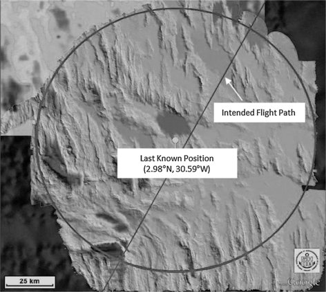
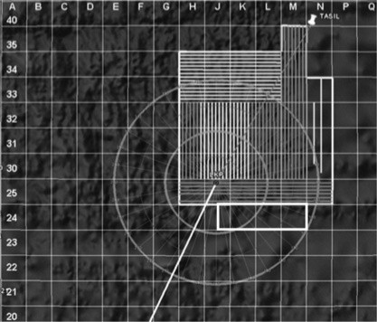
In the early morning hours of June 1, 2009, Air France Flight AF 447, with 228 passengers and crew aboard, disappeared during stormy weather over the Atlantic while on a flight from Rio de Janeiro to Paris. Upon receiving notification of the crash, the French Bureau d’Enquêtes et d’Analyses (BEA) pour la sécurité de l’aviation and French search and rescue authorities organized an international search by aircraft and surface ships to look for signs of the plane and possible survivors. On the sixth day of this effort, the first debris and bodies were found 38 NM north of the aircraft’s last known position. That day a large portion of the galley was found along with other debris and some bodies. Figure 1 shows the aircraft’s last known position, intended flight path and a 40 NM circle about the last known position. Analysis by the BEA determined that the wreckage had to lie within 40 NM of the plane’s last known position.

Figure 1: Last known position of the aircraft, intended flight path and the 40 NM circle.

The aircraft was equipped with a flight data recorder and a cockpit voice recorder. Each of these recorders was fitted with an underwater locator beacon that activates an acoustic signal upon contact with water. The BEA initiated a search to detect these beacons. The search was performed by two ships employing passive acoustic sensors supplied by the U.S. Navy and operated by personnel from Phoenix International. The search began on June 10, 2009 and lasted 31 days until the time when the batteries in the beacons were estimated to be exhausted. The ships searched extensively along the intended flight path, but the beacons were not detected. Next the BEA began an active acoustic search with side-looking sonar to detect the wreckage on the ocean bottom. This search took place in August 2009 south of the last known position in an area not covered by the passive acoustic search. This search was also unsuccessful.

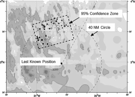
After the unsuccessful search in 2009, the BEA commissioned a group of oceanographic experts to estimate the currents in the area at the time of the crash and to use these estimates along with the times and locations where the surface search had found bodies and debris in order to estimate the location of the wreckage. In Ollitrault2010 the group recommended the rectangular search area north and west of the last known position shown in Figure 2. This rectangle is described as a $95\%$ confidence zone. The group used available current measurements to make a number of estimates of the currents in the area of the wreck at the time of the loss. Using these estimates, they performed a backward drift on recovered debris and bodies to produce a number of trajectories ending at an estimated location of the crash. The group removed trajectories that they felt were outliers. A bivariate normal error was estimated for each of the remaining crash location estimates and used to produce a weighted mean with a bivariate normal error distribution. This error distribution was used to compute a rectangle centered at the mean with a $95\%$ probability of “containing” the wreck location. This rectangle guided the active acoustic search in April and May of 2010.

Figure 2: The $95\%$ confidence zone recommended in Ollitrault2010 for the 2010 search area.

The 2010 searches were performed by two teams. The U.S. Navy and Phoenix International team used a towed side-scan sonar system. The Woods Hole Oceanographic Institute team used autonomous underwater vehicles with side-scan sonars and a remotely operated vehicle. After an unsuccessful search in the rectangle, the teams extended their efforts to the south and west of the rectangle. Unfortunately, this search was also unsuccessful.

In July 2010 we were tasked by the BEA to review all information about the loss of AF 447 as well as the previous search efforts to produce a probability distribution (map) for the location of the underwater wreckage. The probability maps that resulted from this process were used to guide the 2011 search.

On April 3, 2011, almost two years after the loss of the aircraft, the underwater wreckage was located on the ocean bottom some 14,000 feet below the surface. On April 8, 2011, the director of the BEA stated, “This study StoneEtAl2011BEA published on the BEA website on 20 January 2011, indicated a strong possibility for discovery of the wreckage near the center of the Circle. It was in this area that it was in fact discovered after one week of exploration” Troadec2011 . Subsequently, the flight data recorder and cockpit voice recorder were found, retrieved from the ocean bottom and flown to the BEA in Paris where the data in these recorders were recovered and analyzed. This data provided crucial information for determining the cause of the crash. Finding the wreckage also allowed the BEA to return the bodies of many passengers and crew to their loved ones.

In the sections below we describe the Bayesian process used to compute these probability distributions.

2 Why Bayesian Analysis

Bayesian analysis is ideally suited to planning complicated and difficult searches involving uncertainties that are quantified by a combination of objective and subjective probabilities. This approach has been applied to a number of important and successful searches in the past, in particular, the searches for the USS Scorpion RichardsonAndStone1971 and SS Central America Stone1992 . This approach is the basis for the U.S. Coast Guard’s Search and Rescue Optimal Planning System (SAROPS) that is used to plan Coast Guard maritime searches for people and ships missing at sea Fusion2010 .

Complicated searches such as the one for AF 447 are onetime events. We are not able to recreate the conditions of the crash 1000 times and record the distribution of locations where the aircraft hits the water. As a result, definitions of probability distributions in terms of relative frequencies of events do not apply. Instead, we are faced with computing a probability distribution on the location of the wreckage (search object) in the presence of uncertainties and conflicting information that require the use of subjective probabilities. The probability distribution on which the search is based is therefore a subjective one. It is based on the analysts’ best understanding of the uncertainties in the information about the location of the search object.

In an ideal situation, search effort is applied in an optimal fashion to maximize the probability of detecting the search object within the effort available. The optimal search problem is a Bayesian decision problem often based on a subjective probability distribution DeGroot2004 , Koopman1956I , Koopman1956II , Stone2004 . The basic optimal search problem can be stated as follows.

The search object is located in one of $J$ cells with $p(j)$ being the probability the object is in cell $j$. We assume $\sum_{j=1}^{J}{p(j)}=1$. For each cell $j$, there is a detection function $b_{j}$ where ${b_{j}}(z)$ is the probability of detecting the object with effort $z$ given the object is in cell $j$. Search effort is often measured in hours, which we will use for this discussion. A search allocation $Z$ specifies the effort $z_{j}\geq 0$ to be placed in cell $j$ for $j=1,\ldots,J$. The probability of detection $\mathcal{P}(Z)$ and cost $\mathcal{C}(Z)$ for the search allocation $Z$ are computed by

$$\mathcal{P}(Z)=\sum_{j=1}^{J}{{b_{j}}({z_{j}})}p(j)\quad\mbox{and}\quad\mathcal{C}(Z)=\sum_{j=1}^{J}{{z_{j}}}.$$

Suppose there are $T$ hours of search available. The optimal search problem is to find an allocation $Z^{*}$ for which $\mathcal{C}(Z^{*})\leq T$ and

$$\mathcal{P}\bigl{(}Z^{*}\bigr{)}\geq\mathcal{P}(Z)\quad\mbox{for all }Z\mbox{ such that }\mathcal{C}(Z)\leq T.$$

As the search proceeds and the search object is not found, the posterior distribution given failure of the search is computed and used as the basis for planning the next increment of search. Even at this stage, subjective estimates of the detection capability of the sensors must often be used because of the lack of previous testing against the search object. Classical statistics has no formalism for approaching this type of decision problem. In contrast, Bayesian statistics and decision theory are ideally suited to the task.

3 Analysis Approach

In the analysis that we performed for the BEA, we were not called upon to provide a recommended allocation of search effort but only to compute the posterior distribution for the location of the wreckage. The approach taken for this analysis follows the model described in RichardsonAndStone1971 and Stone1992 . The information about a complex search is often inconsistent and contradictory. However, one can organize it into self-consistent stories or scenarios about the loss of the aircraft. Within each scenario, the uncertainties in the information are quantified using probability distributions. These distributions may be subjective if little or no data is available to estimate the uncertainties. For each scenario, a probability distribution on target location is computed to reflect the uncertainties in the information forming the scenario. This is typically done by simulation. The resulting distributions are combined by assigning subjective probabilities to the scenarios and computing a weighted mixture of these scenario distributions to obtain the prior distribution. The subjective probability assigned to a scenario reflects the analysts’ evaluation of the probability that the scenario represents what happened.

We approximated the continuous spatial distribution for the location of the wreckage by a discrete distribution represented by a set of $N$ point masses or particles $(x_{n},w_{n})$ for $n=1,\ldots,N$, where $w_{n}$ is the probability mass attached to particle $n$. The probabilities sum to 1. In the case of a stationary search object, $x_{n}$ is a latitude-longitude point. In the case of a moving object, $x_{n}$ is a continuous space and time path over the time interval of interest. For visualization purposes, a grid of cells is imposed on the search space. Cell probabilities are computed by summing the probabilities of the particles in each cell, and the cells are color coded according to their probabilities. For the figures in this paper we used a black to white scale with black indicating the highest probability cells and white the lowest. Computation of the probability distributions described below was performed by a modified version of SAROPS.

The computation of the posterior distribution involves two basic steps, (1) computation of the prior (before search) distribution and (2) computation of the posterior distribution given the unsuccessful search.

3.1 Prior Distribution

During flight, a commercial aircraft sends messages via satellite containing maintenance and logistic information about the aircraft. Every 10 minutes it sends a GPS position for the aircraft. The last known position, $2.98^{\circ}$N latitude$/$$30.59^{\circ}$W longitude, for AF 447 was sent at 02 hours 10 minutes and 34 seconds Coordinated Universal Time on June 1, 2009. Based on failure to receive any messages after 02 hours, 14 minutes and 26 seconds, the BEA estimated that the plane could not have traveled more than 40 NM from its last known position before crashing into the ocean. Thus, we assumed the location of the wreckage was within the 40 NM circle centered at the last known position with probability 1. Any probability distribution for the location of the wreckage that had probability outside this circle was truncated at the circle and renormalized to a probability distribution. Errors in GPS positions typically have a standard deviation of roughly 10 m which is dwarfed by the other uncertainties in the location of the aircraft, so this error was not considered to be significant in our analysis.

The prior distribution $P$ on the location of the wreck was taken to be a mixture of three distributions, $D_{1}$, $D_{2}$ and $D_{3}$. The distribution $D_{1}$ is uniform within the 40 NM circle, and $D_{2}$ is based on data from crashes that involved loss of control while a plane was at flight altitude. $D_{3}$ is based on an analysis that drifted dead bodies found on the surface backward in time to possible crash locations. On the basis of discussions with analysts at the BEA, we decided on the following subjective weights for these distributions (scenarios), $p_{1}=p_{2}=0.35$ and $p_{3}=0.3$ so that

$$P=p_{1}D_{1}+p_{2}D_{2}+p_{3}D_{3}.$$ (1)

In retrospect, it appears it would have been more appropriate to view $D_{3}$ as a likelihood function and multiply the distribution $0.5D_{1}+0.5D_{2}$ by $D_{3}$ to obtain the prior.

The distribution $D_{2}$ is based on an analysis of data from nine commercial aircraft accidents involving loss of control at flight altitude. The analysis was performed by the Russian Interstate Aviation Group and the BEA. It showed that all impact points (adjusted to the 35,000-foot altitude at which AF 447 was cruising) were contained within a circle of radius 20 NM from the point at which the emergency began. These results were represented by a circular normal distribution centered at the last known position with standard deviation 8 NM along any axis. We set $D_{2}$ equal to this distribution truncated at the 40 NM circle.

The $D_{3}$ scenario is the reverse-drift scenario. The distribution for this scenario was computed using data on currents and winds to reverse the motion of recovered bodies back to the time of impact. We used current estimates produced for BEA Ollitrault2010 and wind estimates from the U.S. Navy’s Operational Global Atmospheric Prediction System model to perform the reverse drift.

At daylight on June 1st, 2009, French and Brazilian aircraft began a visual search for survivors and debris from the wreck. The first debris was found on June 6th, and more than 60 bodies were recovered from June 6th–June 10th, 2009.

There are two components of drift, drift due to ocean current and drift due to wind. The latter is called leeway. To produce the reverse-drift scenario, we used positions and times at which bodies were recovered from June 6–10. We did not reverse-drift pieces of debris because we lacked good leeway models for them, whereas we could use the model in Breivik2011100 for bodies. We used polygons to represent the positions of selected bodies recovered on each day from June 6–10. For each polygon 16,000 positions were drawn from a uniform distribution over the polygon. Each position became a particle that was drifted backward in time subject to winds and currents in the following manner. We used a 60-minute time step. For each step and each particle, a draw was made from the distributions on wind and current for the time and position of the particle in the manner described below. The negative of the vector sum of current plus the leeway resulting from the wind was applied to the particle motion until the next time step.

Figure 3: Reverse drift distribution $D_{3}$.

Figure 4: Prior distribution $P$.

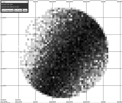
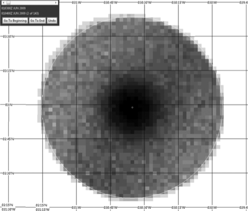
The large uncertainties in the ocean currents at the time of the crash produced a distribution for the crash location that spread way beyond the 40 NM circle. Figure 3 shows the reverse-drift distribution produced in this fashion and truncated at the 40 NM circle. Because of the large uncertainties in the currents, this scenario was given a lower weight than the other two that comprise the prior. Figure 4 shows the prior $P$. For the prior distribution and the subsequent posteriors given failure to detect, we used $N=75\mbox{,}000$ points.

3.1.1 Simulating winds and currents

This section discusses simulation of winds and currents.

Wind and current estimates are provided by the environmental community in the form of a grid of velocity vectors $(u,v)$ indexed by space and time where $u$ is the speed in the east–west direction and $v$ is the speed in the north–south direction. We interpret these as mean values of the actual wind and current velocities and add a stochastic component by the method described below.

To obtain $(u,v)$ for a wind or current at a time that corresponds to a grid time but for a spatial point that is not equal to one of the spatial grid points, we take the three closest spatial grid points and use a weighted average of the values at those points, where the weights are proportional to the inverses of the distances from the desired point to the chosen grid points.

Most often we will need $(u,v)$ for times that are not equal to one of the time grid values. To get $(u,v)$ in this case, we use the values as calculated above for the two closest times in the data and then linearly interpolate between these values.

For every time step and every particle, the simulation perturbs the speeds $u$ and $v$ obtained from the data by adding a random draw from a normal distribution with a standard deviation of 0.22 kts for current speeds and 2.0 kts for wind speeds. These draws are independent for $u$ and $v$ and from particle to particle, but for a given particle and speed the draws are correlated in time. Specifically, if $\Delta t$ is the increment in time, measured in minutes, between two time steps, then the correlation is given by

$$\rho(\Delta t)=e^{-\alpha\Delta t},$$

where $\alpha$ is chosen so that $e^{-\alpha 60}=1/2$.

3.1.2 Simulating drift

There are two forces acting on a drifting particle: currents and winds. The effect of current is straightforward. The particle’s velocity due to the current is equal to the velocity of the current.

While it is reasonable to expect that a current of 3 knots will push an object at a speed of 3 knots, the same is not true for the wind. Drift due to wind (leeway) results from the sum of the force of the wind acting on the exposed surfaces of the object and the drag of the water acting on the submerged surfaces of the object.

The wind does not push an object at the wind’s speed, and it often does not push an object exactly in the downwind direction. There is typically a downwind and crosswind component of leeway. The downwind component is in the direction the wind is blowing. The crosswind component is perpendicular to the downwind component, and the direction of the crosswind leeway is not predictable. To account for this, the simulation switches between the two crosswind directions at exponentially distributed times as it is producing a particle path. The magnitudes of the downwind and crosswind components are computed as follows.

For a given particle and time, we compute the wind velocity from the gridded wind data in the same fashion as for the ocean currents. Let $W$ be resulting wind speed expressed in meters per second. For a deceased person floating in the water, we used the following model developed in Breivik2011100 to compute the mean downwind leeway $\mathit{DW}$ and crosswind leeway $\mathit{CW}$ measured in centimeters per second (cm/s):

$$\mathit{DW} = 1.17W+10.2\mbox{ cm/s},$$

$$\mathit{CW} = 0.04W+3.9\mbox{ cm/s}.$$

We added a random component to the mean values computed above by adding the value of a draw from a normal distribution with mean 0 and standard deviation equal to the standard error computed for the regression used to estimate the mean downwind and crosswind leeway, respectively. The time correlation of the random components of leeway was handled in the same way as for the ocean currents.

3.2 Posterior Distribution

The posterior distribution was computed in four steps with each step accounting for an increment of unsuccessful search. The result is the posterior distribution on the wreck location given failure of the search effort in 2009 and 2010. The steps, that is, increments of unsuccessful search, are listed below:

1. Failure of the surface search to find debris or bodies for almost 6 days during June 1–6, 2009.

2. Failure of the passive acoustic search to detect the underwater locator beacons on the flight data recorder and cockpit voice recorder in June and July 2009.

3. Failure of the active side-looking sonar search for the wreckage in August 2009.

4. Failure of the active side-looking sonar search for the wreckage in April and May of 2010.

We use the following notation for the posterior distributions. $\tilde{P}_{1}$ denotes the posterior given failure of search increment 1; $\tilde{P}_{12}$ denotes the posterior given failure of search increments 1 and 2, and so on to $\tilde{P}_{1234}$ which denotes the posterior given failure of search increments 1–4. It is $\tilde{P}_{1234}$ that the BEA used to plan the successful 2011 search. These distributions were computed sequentially. First $\tilde{P}_{1}$ was computed and used as the “prior” for computing $\tilde{P}_{12}$. Then $\tilde{P}_{12}$ was used as the prior to compute $\tilde{P}_{123}$ and so on.

4 Computing the Posteriors

In this section we describe how we accounted for the four increments of unsuccessful search by computing the posterior distributions described above.

4.1 Accounting for Unsuccessful Search

We represented the prior distribution $P$ by making $N=75\mbox{,}000$ independent draws from this distribution for the location of the wreck on the ocean bottom. For the $n$th particle we set $x_{n}$ equal to the location of the $n$th draw and $w_{n}=1/N$ for $n=1,\ldots,N$. If an unsuccessful search takes place, we compute the probability $p_{d}(n)$ that the search would have detected the search object if it were located at $x_{n}$. The posterior probabilities $\tilde{w}_{n}$ on the particles are computed using Bayes’ rule as follows:

$$\tilde{w}_{n}=\frac{(1-p_{d}(n))w_{n}}{\sum_{n^{\prime}=1}^{N}(1-p_{d}(n^{\prime}))w_{n^{\prime}}}$$ (3)

$$\eqntext{\mbox{for }n=1,\ldots,N.}$$

The updated particles $(x_{n},\tilde{w}_{n})$ for $n=1,\ldots,N$ provide a discrete approximation to the posterior given failure of the search.

If the search object is moving, then a stochastic motion model must be specified. In addition to drawing the initial position, we make draws from the distributions specified by the motion model to create a continuous time and space path for the search object over the time interval of interest. Each particle is a path with a probability on it. The set of particles is a discrete sample path approximation to the stochastic process describing the motion of the search object. When a search takes place, we account for the motion of the particles and the sensors in calculating $p_{d}(n)$. The posterior is again computed from (3).

4.2 Step 1: Unsuccessful Surface Search

We decided to incorporate the effect of the almost 6 days of unsuccessful surface search as follows. Each point $x_{n}$ in the prior specifies a location on the ocean bottom. In the calculation of this distribution, we assumed that when the aircraft crashed into the surface of the ocean it fell straight to the bottom some 14,000 feet below. It is likely that there was some lateral motion as the wreckage drifted to the bottom, but we reasoned that this uncertainty was small compared to the other uncertainties in the problem, so we ignored it.

For each particle we constructed a path starting at the position of the particle projected up to the surface of the ocean. We drifted the particle forward in time for six days using the wind and current drift model described in Section 3.1. However, this time we used the drift vector itself rather than its negative. This produced a path for each particle. As with the reverse drift scenario, the leeway component of drift was based on that of a body in the water.

Aircraft searches are reported in terms of sorties. Sorties described a sequence of straight line segments (flight legs) flown at specified times, speeds and altitudes. Typically the set of legs for a sortie covers a rectangular area on the ocean surface. We used the detectability of the galley found on the 6th day of surface search as a surrogate for the detectability of the floating debris. We further assumed that the detectability of the galley is equivalent to that of a four-man raft (they are roughly the same size). The Coast Guard has developed tables that provide estimates of the probability of detecting a four-man raft from an aircraft on one leg of a sortie as a function of the speed and altitude of the aircraft, range at the point of closest approach to the search object on the leg, and environmental variables such as visibility, cloud cover and sea state of the ocean.

For each particle and each leg of each sortie, we computed the range at closest point of approach and used the Coast Guard tables to compute the probability that the particle would fail to be detected on that leg. We assumed an independent detection opportunity on each leg and multiplied the failure probability for each leg and sortie to obtain an overall probability of failure to detect for each particle. Search by ships was incorporated in a similar manner. The result was the computation of the failure probability $q(n)$ for the air and ship searches for each particle for the six days of unsuccessful search.

Because of the many uncertainties and approximations involved in the computation of the failure probabilities for this search, and because we felt that it was unlikely that the search would fail to detect any debris for almost six days under the assumptions we had made, we decided it was necessary to allow for the possibility that the search was ineffective for most of those six days for reasons unknown to us. We made a subjective estimate that the search was ineffective (failure probability 1) with probability 0.7 and effective [failure probability $q(n)$] with probability 0.3. As a result we set $1-p_{d}(n)=0.7+0.3q(n)$ and computed the posterior probabilities $w_{n}^{1}=\tilde{w}_{n}$ on the path of the $n$th particle by (3), which is also the posterior probability on the wreck location being equal to $x_{n}$ given failure of the six days of surface search. Thus, $(x_{n},w_{n}^{1})$ for $n=1,\ldots,N$ yields the posterior distribution $\tilde{P}_{1}$. More details on the aircraft searches may be found in StoneEtAl2011BEA .

Figure 5: The vertical and horizontal lines show the search paths for the passive acoustic search. The circles are the 20 and 40 NM circles about the last known position. The white rectangle in row 24 was searched by side-looking sonar in August 2009.

4.3 Step 2: Passive Acoustic Search for the Underwater Locator Beacons

The aircraft was equipped with a flight data recorder and a cockpit voice recorder. Each of these recorders was fitted with an underwater locator beacon that activates an acoustic signal upon contact with water. The batteries on the locator beacons were estimated to last for 40 days.

The passive acoustic search to detect these beacons lasted 31 days ending on 10 July 2009. The search was performed by two ships employing passive acoustic sensors supplied by the U.S. Navy and operated by personnel from Phoenix International. Based on a calculation involving the source level of the beacons and propagation loss through the water, we estimated the sensors to have probability at least $0.9$ of detecting the beacons within lateral range 1730 m. Experience in past searches has shown that detection estimates based on manufacturers’ specifications and operator estimates tend to be optimistic. Thus, we put a maximum of 0.9 on estimates of sensor detection probabilities. The search paths, which are shown in Figure 5, were designed so that 1730 m would be the maximum lateral range to the nearest path for any point in the search region.

In estimating the probability of detection for these sensors we accounted for the possibility that one or both of the beacons were destroyed in the crash. Based on survival data for these beacons obtained from previous crashes, we estimated a probability of 0.8 that a single beacon survived the crash. If beacon survival is independent, then $P_{D}$, the probability of detecting at least one of the beacons given they are within lateral range 1730 m of the sensor, equals

$$P_{D}=\bigl{(}1-(0.1)^{2}\bigr{)}(0.8)^{2}+(0.9)\bigl{(}2(0.8)(0.2)\bigr{)}=0.92.$$

If the beacons were mounted sufficiently close together to consider their chances of survival to be completely dependent, then the probability of detecting at least one beacon drops to $0.9\times 0.8=0.72$. We decided to use a weighted average of 0.25 for the independent and 0.75 for the dependent probabilities, yielding a detection probability of $\bar{P}_{D}=77$.

Figure 6: Regions searched by active side-looking sonar in April–May 2010.

The ships tracks displayed in Figure 5 show the passive acoustic search paths, which were designed to cover the expected flight path of the aircraft. We computed the posterior distribution $\tilde{P}_{12}$ by starting with $\tilde{P}_{1}$ as the prior and computing $1-p_{d}(n)$ for each particle by the same method used for the aircraft search. For each particle and path, we determined whether the path came within 1730 m of the particle. If it did, the failure probability for that particle was multiplied by $1-\bar{P}_{D}=0.23$. The resulting $1-p_{d}(n)$ was used in (3) with $w_{n}=w_{n}^{1}$ to compute $w_{n}^{2}=\tilde{w}_{n}$ and the posterior distribution $\tilde{P}_{12}$.

4.4 Step 3: Active Side-Looking Sonar Search in August 2009

The BEA employed a side-looking (active) sonar from the French Research Institute for Exploration of the Seas towed by the French research vessel Pourquoi Pas? to continue the search after the batteries on the beacons were estimated to have been exhausted. This search took place in August 2009 in the white rectangle in row 24 in Figure 5. This region was chosen because it was suitable for search by side-looking sonar and had not been searched before. We assumed a 0.90 probability of detection in the searched region. This represents a conservative, subjective estimate of the probability of this sensor detecting a field of debris. The detection of small items such as oil drums on the ocean bottom confirmed that the sensor was working well. We computed the posterior after this search effort by setting

$$\qquad 1-p_{d}(n)=\cases{0.1,&if $x_{n}$ is located in the\cr&search rectangle,\cr 1,&otherwise.}$$ (4)

This $1-p_{d}(n)$ was used in (3) with $w_{n}=w_{n}^{2}$ to compute $w_{n}^{3}$ and the posterior distribution $\tilde{P}_{123}$.

Figure 7: Posterior distrubtion $\tilde{P}_{1234}$.

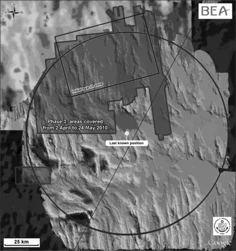
4.5 Step 4: Active Side-Looking Sonar Search in April and May 2010

Figure 6 shows the regions searched during 2010 with active side-looking sonar. The search began in the rectangular region recommended by Ollitrault2010 inside the 40 NM circle and proceeded to the remainder of the areas shown in medium gray including a small rectangular region southwest of the last known position. As with the previous active sonar search, we estimated that within these regions the search sensors achieved detection probability 0.9. We felt this was a conservative subjective estimate based on the careful execution of the search, the quality of sonar records and the numerous small articles detected during this search. The search region was represented by a rectangular and a polygonal region. As with the active sonar search in 2009, we computed $1-p_{d}(n)$ in the manner given in (4) with the rectangular and polygonal search regions replacing the rectangle of the 2009 search. This produced the desired posterior $\tilde{P}_{1234}$ which accounts for all the unsuccessful search.

4.6 Posterior After the Unsuccessful Searches in Steps 1–4

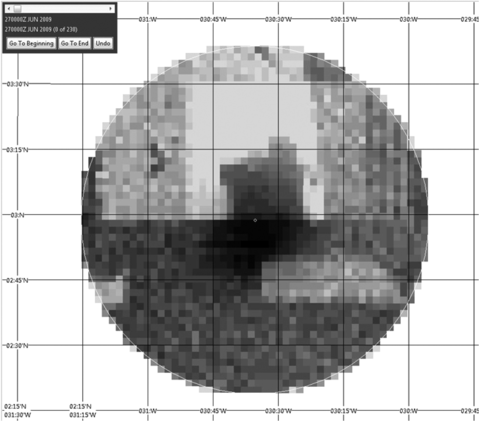
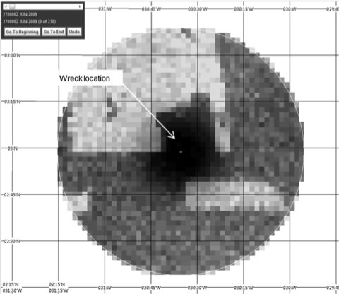
Figure 7 shows the posterior after the unsuccessful searches in steps 1–4. Even though this posterior allows for the possibility that the beacons did not work, doubts about the beacons compelled us to produce the alternate posterior shown in Figure 8, which assumes the beacons did not function. The location of the wreckage which is shown in this figure falls in a high probability area. This posterior distribution seems remarkably accurate and raises the question of why the beacons were not detected.

The BEA recovered one data recorder with the beacon attached. Testing by the BEA showed that when the beacon was connected to a fully charged battery, it did not produce a signal. This indicates that the beacons were damaged in the crash and did not function. This would explain why the beacons were not detected by the passive acoustic search.

A better way to handle the doubts that we had about the beacons would have been to compute a joint distribution on beacon failure and wreck location. The marginal distribution on wreck location would then be the appropriate posterior on which to base further search.

Figure 8: Posterior distribution which assumes both beacons failed; produced because of doubts about the survivability of the beacons.

5 Conclusions

Figure 8 shows that the wreckage is located in a high probability area assuming the beacons failed to operate properly. Because the wreckage is located in an area thoroughly covered by the passive search (see Figure 5), these results and the tests of the recovered beacon by the BEA suggest that both beacons failed to actuate. It appears that the likely failure of the beacons to actuate resulted in a long and difficult search.

The approach described in this paper used a careful and methodical consideration of all data available with their associated uncertainties, to form an analytic assessment of the highest likelihood areas for future search efforts. The weighted scenario approach allowed inconsistent information to be combined with subjective weights that capture the confidence in the data. The analysis of the detection effectiveness of each search component produced the Bayesian posterior distributions shown in Figures 7 and 8 and formed a solid basis for planning the next increment of search. In fact, the 2011 search commenced in the center of the distribution and quickly found the wreckage.

Failure to use a Bayesian approach in planning the 2010 search delayed the discovery of the wreckage by up to one year. The success of the analysis described in this paper provides a powerful illustration of the value of a methodical, Bayesian approach to search planning. The full report of this work is available on the BEA website in StoneEtAl2011BEA .