Constraints on the progenitor system and the environs of SN 2014J
from deep radio observations

Abstract

We report deep EVN and eMERLIN observations of the Type Ia SN 2014J in the nearby galaxy M 82. Our observations represent, together with JVLA observations of SNe 2011fe and 2014J, the most sensitive radio studies of Type Ia SNe ever. By combining data and a proper modeling of the radio emission, we constrain the mass-loss rate from the progenitor system of SN 2014J to $\dot{M}\lesssim 7.0\times 10^{-10}~{}\mbox{\,${\rm M_{\odot}\,yr^{-1}}$}$ (for a wind speed of $100\mbox{\,km s${}^{-1}$}$). If the medium around the supernova is uniform, then $n_{\rm ISM}\lesssim 1.3\mbox{\,cm${}^{-3}$}$, which is the most stringent limit for the (uniform) density around a Type Ia SN. Our deep upper limits favor a double-degenerate (DD) scenario–involving two WD stars–for the progenitor system of SN 2014J, as such systems have less circumstellar gas than our upper limits. By contrast, most single-degenerate (SD) scenarios, i.e., the wide family of progenitor systems where a red giant, main-sequence, or sub-giant star donates mass to a exploding WD, are ruled out by our observations. Our estimates on the limits to the gas density surrounding SN2011fe, using the flux density limits from Chomiuk et al. (2012), agree well with their results. Although we discuss possibilities for a SD scenario to pass observational tests, as well as uncertainties in the modeling of the radio emission, the evidence from SNe 2011fe and 2014J points in the direction of a DD scenario for both.

1. Introduction

Type Ia supernovae (SNe) are the end-products of white dwarfs with a mass approaching the Chandrasekhar limit, which results in a thermonuclear explosion of the star. In addition to their use as cosmological distance indicators (e.g., Riess et al., 1998; Perlmutter et al., 1999), Type Ia SNe (henceforth SNe Ia) are a major contributor to the chemical evolution of galaxies. It is therefore unfortunate that we do not yet know what makes a SN Ia. This lack of knowledge makes it difficult to gain a physical understanding of the explosions, so that we can model possible evolution, which compromises their use as distance indicators. It also means we do not fully understand the timescale over which SNe Ia turn on, adding a large uncertainty to our understanding of the chemical evolution of galaxies.

Unveiling the progenitor scenario for SNe Ia is difficult because white dwarfs (WDs) can, theoretically, reach their fatal Chandrasekhar mass in many ways, and disentangling which is the correct one (if there is just one), is challenging from an observational point of view. Nonetheless, there are two basic families of models leading to a SN Ia, the single-degenerate model (SD) and the double-degenerate model (DD). In the SD scenario, a WD accretes mass from a hydrogen-rich companion star before reaching a mass close to the Chandrasekhar mass and going off as supernova. In the DD scenario, two WDs merge, with the more-massive WD being thought to tidally disrupt and accrete the lower-mass WD (see, e.g., Maoz et al., 2014, and references therein).

Observations can potentially discriminate between the progenitor models of SNe Ia. For example, in all scenarios with mass transfer from a companion, a significant amount of circumstellar gas is expected (see, e.g., Branch et al., 1995), and therefore a shock is bound to form when the supernova ejecta are expelled. The situation would then be very similar to circumstellar interaction in core-collapse SNe, where the interaction of the blast wave from the supernova with its circumstellar medium results in strong radio and X-ray emission (Chevalier, 1982b). On the other hand, the DD scenario will not give rise to any circumstellar medium close to the progenitor system, and hence essentially no radio emission is expected.

Radio and X-ray observations of SN 2011fe have provided the most sensitive constraints on possible circumstellar material (Chomiuk et al., 2012; Margutti et al., 2012) around a normal SN Ia. The claimed limits on mass loss rate from the progenitor system are $\dot{M}=6\times 10^{-10}$  ${\rm M_{\odot}\,yr^{-1}}$ and $\dot{M}=2\times 10^{-9}$  ${\rm M_{\odot}\,yr^{-1}}$ from radio (Chomiuk et al., 2012) and X-rays (Margutti et al., 2012), respectively, assuming a wind velocity of 100 km s^-1. Radio (e.g., Panagia et al., 2006; Hancock et al., 2011) and X-ray (e.g., Hughes et al., 2007; Russell & Immler, 2012) observations of other, more distant SNe Ia, have resulted in less constraining upper limits on wind density. The non-detections of radio and X-ray emission from SNe Ia have added to a growing consensus that a large fraction of SNe Ia may not be the result of SD scenarios (e.g., Maoz et al., 2014).

Despite the non-detection of radio and X-ray emission, there is evidence of possible circumstellar material in the form of time-varying absorption features in the optical Na I D line for a few SNe Ia (Patat et al., 2007; Simon et al., 2009; Dilday et al., 2012), supposed to arise in circumstellar shells. The exact location of the absorbing gas is still debated (e.g., Chugai, 2008; Soaker, 2014), and probably varies from case to case. The number of SNe Ia showing indications of circumstellar shells could be significant, although the uncertainty is still large ((18$\pm 11$)%; Sternberg et al. 2014). Just as with the radio and X-rays, no optical circumstellar emission lines from normal SNe Ia have yet been detected (e.g., Lundqvist et al., 2013), although there are a few cases with strong emission (see, e.g., Maoz et al., 2014, for an overview). Those SNe Ia with strong circumstellar interaction constitute a very small fraction of all SNe Ia, probably only $\sim 1$% (Chugai et al., 2004).

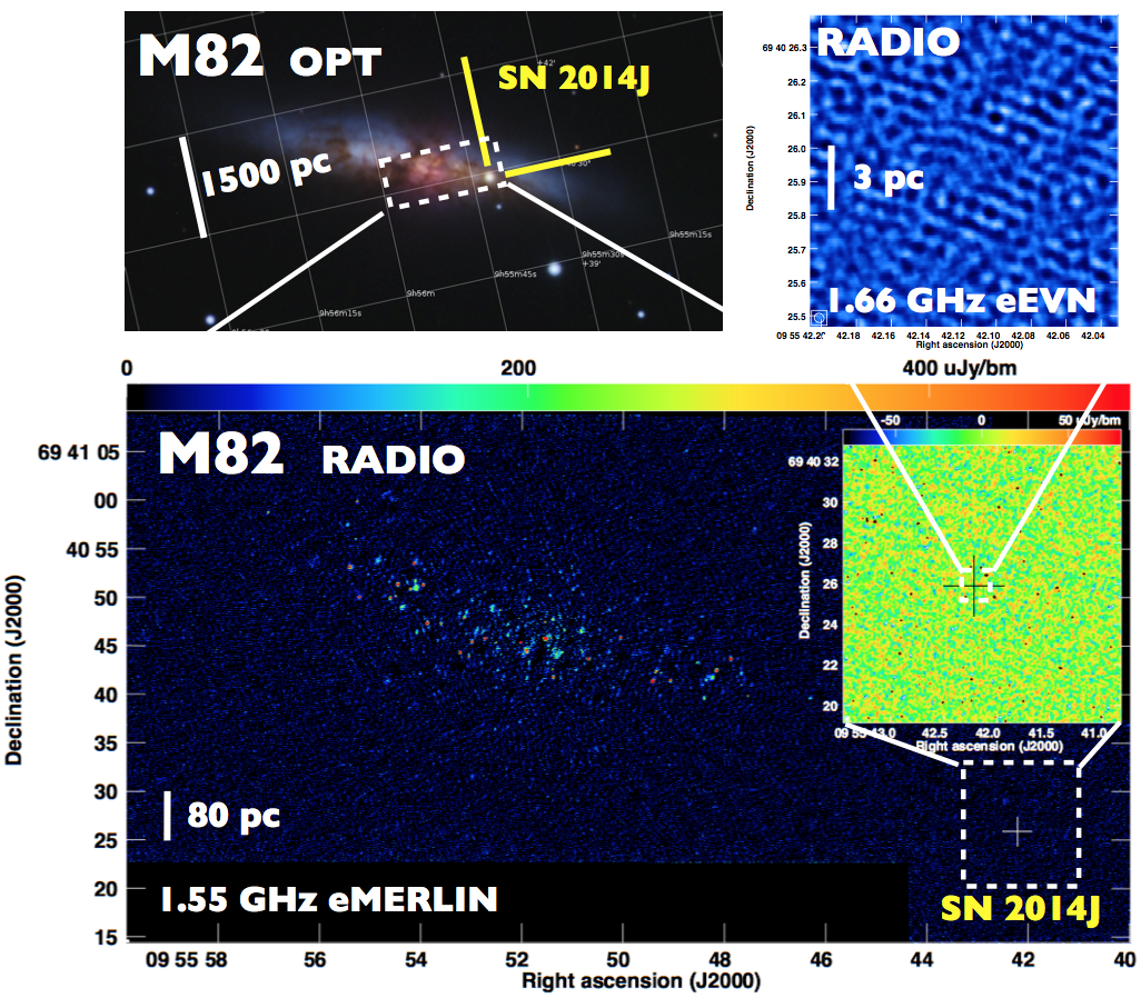
Recently, Fossey et al. (2014) serendipitously discovered SN 2014J in the nearby galaxy M 82 (D=3.5 Mpc). Cao et al. (2014) classified SN 2014J as a SN Ia, which makes it the closest SN Ia since SN 1986G in Cen A, almost three decades ago. The supernova exploded between UT 14.56 Jan 2014 and 15.57 Jan 2014 according to the imaging obtained by Itagaki et al. (2014), and its J2000.0 coordinates are RA=09:55:42.121, Dec=+69:40:25.88 (Smith et al., 2014). For a further discussion on the discovery and early rise of the optical/IR emission, we refer to Goobar et al. (2014) and Zheng et al. (2014). The vicinity of SN 2014J makes it a unique case for probing its prompt radio emission, and thus constrain its progenitor system.

2. Observations and data reduction

We observed SN2014J with the electronic Multi Element Radio Interferometric Network (eMERLIN) at 1.55 and 6.17 GHz, and with the electronic European Very Long Baseline Interferometry Network (EVN) at a frequency of 1.66 GHz. We show in Table 1 the summary for our observations, along with radio data obtained by others.

2.1. eMERLIN observations

We observed SN 2014J with eMERLIN on 28 January 2014, at a frequency of 1.55 GHz, and on 29-30 January 2014, at a frequency of 6.17 GHz. Our observing array included, at both frequencies, all eMERLIN stations (Lovell, Jodrell Mk2, Darham, Pickmere, Cambridge, Defford, Knockin). Given the expected faintness of SN 2014J  we used a phase-reference observing scheme, with $\sim$8 minutes spent on the SN, and $\sim$2 minutes on the nearby, bright phase-calibrator J0955+6903 (RA=09:55:33.1731; Dec=69:03:55.061). We used 3C286 as our absolute flux density calibrator, and OQ208 as bandpass calibrator. We observed in dual-polarization mode at both frequencies. The bandwidth at 1.55 (6.17) GHz was of 512 (1024) MHz. Each of those frequency bands was split into 4 (8) spectral windows (SPW) of 128 MHz each. Each SPW was in turn split into 512 channels/polarisation.

Figure 1.— Top left: RGB optical image of the very nearby galaxy M 82 and its SN 2014J  obtained with the 50 cm telescope of the Observatorio Astronómico de Aras, Spain, on 31 January 2014. Bottom: 1.55 GHz eMERLIN radio image of M 82 from our observations on 28 January 2014, which shows a large number of supernovae and supernova remnants. The inset is a blow-up image of the region around SN 2014J. Top right: 1.66 GHz eEVN image of the SN 2014J field.

Table 1Log of radio observations

Starting	$T$	$t_{\rm int}$	Array	$\nu$	$S_{\nu}$	Lν,23	$\dot{M}_{-9}$
UT	day	hours		GHz	$\mu$Jy
Jan 23.2	8.2	$-$	JVLA	5.50	12.0	1.77	0.70 (4.2)
Jan 24.4	9.4	$-$	JVLA	22.0	24.0	3.51	3.7 (22)
Jan 28.8	13.8	13.6	eMERLIN	1.55	37.2	5.46	1.15 (7.0)
Jan 29.5	14.5	14.0	eMERLIN	6.17	40.8	5.97	3.6 (22)
Feb 4.0	20.0	11.0	eEVN	1.66	32.4	4.74	1.69 (10)
Feb 19.1	35.0	10.0	eEVN	1.66	28.5	4.17	2.9 (16)

We loaded the data into the NRAO Astronomical Image Processing System (AIPS) of the National Radio Astronomy Observatory (NRAO, USA), after having averaged them to 128 channels per SPW (i.e., channel width of 500 kHz). We used AIPS for calibration, data inspection, and flagging, using standard procedures. We lost $\sim$15% of the data due to Radio Frequency Interference (RFI). We imaged the $\sim$13′($\sim$4′) field of view of our 1.55 (6.17) GHz observations, including M82, which has a strong and spatially complex radio structure, using a robust=0 uv-weighting scheme. We used those in-beam radio sources to refine the target field calibration via several rounds of phase and amplitude self-calibration. Following these rounds of self-calibration, we reweighted the target visibilities to account for difference in the sensitivity of the individual e-MERLIN antennas. Our final imaging yielded 13.6 and 12.4 $\mu$Jy/bm r.m.s. noise levels at the location of SN2014J at 1.55 and 1.67 GHz, respectively.

2.2. eEVN observations

We observed our target source, SN 2014J on 3-4 February 2014 and 19 February 2014, using the eEVN at 1.66 GHz. We used a sustained data recording rate of 1024 Mbit s^-1, in dual-polarisation mode and with 2-bit sampling. Each frequency band was split into 8 intermediate subbands of 16 MHz bandwidth each, for a total synthesized bandwidth of 128 MHz. Each subband was in turn split into 128 (64) spectral channels of 125 (250) kHz bandwidth each for the observations on 3-4 February (19 February) 2014.

Our observations on 3 February included the following six antennas of the EVN: Effelsberg, Westerbork (phased array), Jodrell Bank (Mk 2), Medicina, Onsala, and Torun. In addition to these antennas, our observing run on 19 February included also the antennas of Noto and Sheshan. We observed our target source, SN 2014J, phase-referenced to the core of the nearby galaxy M81, known to be very compact at VLBI scales, with a typical duty cycle of 5 minutes. We used the strong source DA193 as fringe finder and bandpass calibrator. All the data were correlated at the EVN MkIV data processor of the Joint Institute for VLBI in Europe (JIVE, the Netherlands), using an averaging time of 1 s.

We used AIPS for calibration, data inspection, and flagging of our eEVN data, using standard procedures. Those steps included a-priori gain calibration (using the measured gains and system temperatures of each antenna), parallactic angle correction and correction for ionosphere effects. We then aligned the visibility phases in the different subbands, i.e., “fringe-fitted” the data, solved for the residual delays and delay rates, and interpolated the resulting gains into the scans of SN 2014J. We then imaged a field of view of 3″$\times$3″centered at the position given by Smith et al. (2014), and applied standard imaging procedures using AIPS, without averaging the data either in time, or frequency, to prevent time- and bandwidth smearing of the images. We used natural uv-weighting to maximize the signal to noise ratio in our final images.

3. A model for the radio emission from Type Ia SNe

The radio and X-ray non-detections of SNe Ia, in conjunction with indications of circumstellar shells around some SNe Ia (see §1), is a conundrum that yet has to find a solution. The nearby northern hemisphere SNe 2011fe and 2014J offer a possibility to use the most sensitive radio facilities present to probe circumstellar emission. In particular, we now interpret the upper limits on radio emission from SN 2014J in §2 within the framework of circumstellar interaction. Indeed, when the supernova shock-wave ploughs through the circumstellar gas, a high-energy density shell forms. Within this shell, electrons are accelerated to relativistic speeds and significant magnetic fields are generated, especially if the circumstellar gas is pre-ionized. For the low wind densities discussed in this paper, pre-ionization is likely to occur (Cumming et al., 1996). The relativistic electrons radiate synchrotron (radio) emission (e.g., Chevalier, 1982b).

A proper modeling of the radio emission from SNe requires, in principle, taking into account Coulomb, synchrotron, and (inverse) Compton losses of the relativistic electrons. However, since we only have upper limits for the radio emission from SN 2014J, we will discuss the radio emission from SNe Ia within a scenario of Type Ib/c SNe (see, e.g., Chevalier & Fransson, 2006), neglecting energy losses for the relativistic electrons (c.f. Fransson & Björnsson, 1998; Martí-Vidal et al., 2011, for a more general treatment). The spectrum of the radio emission from those SNe follows the “Synchrotron Self-Absorption” (SSA) form, i.e., a rising power law with $\nu^{5/2}$ (low-frequency, optically thick regime), and a declining power law, $\nu^{\alpha}$ (high frequency, optically thin regime), where $\alpha$ is assumed to be constant. For most well studied SNe, $\alpha\approx-1$ (Chevalier & Fransson, 2006). We assume that electrons are accelerated to relativistic energies, with a power law distribution, $dN/dE=N_{0}E^{-p}$; where $E=\gamma m_{e}c^{2}$ is the energy of the electrons and $\gamma$ is the Lorentz factor. For synchrotron emission, $\alpha=(p-1)/2$, which indicates that $p\approx 3$ should be used.

Here, we study both the case of a circumstellar structure created by a wind, as well as the case with constant density circumstellar gas. For the wind case, we make the standard assumption that the SN progenitor has been losing matter at a constant rate, $\dot{M}$, so that the circumstellar density has a radial profile: $\rho(r)=n_{\rm CSM}(r)\mu=\dot{M}/(4\pi r^{2}v_{w})$, where $v_{w}$ is the wind velocity, $r$ is the radial distance from the star, $n(r)$ is the particle density and $\mu$ is the mean atomic weight of the circumstellar matter.

To calculate the shock expansion, we use the thin-shell approximation (Chevalier, 1982b), with the extensions of Truelove & McKee (1999). We assume that the innermost ejecta has a density slope of $\rho_{\rm ej,inner}\propto r^{-\delta}$, which at some velocity of the ejecta rolls over to a steeper density profile, $\rho_{\rm ej,outer}\propto r^{-n}$ ($n>\delta$). We assume $\delta=-2$, motivated by the explosion models of Fink et al. (2014), and use $n=10.2$, which is a good approximation to the outer density profile of a supernova that stems from a radiative star (Matzner & McKee, 1999). Assuming an ejecta mass of $1.4~{}\hbox{M${}_{\odot}$}$ and a kinetic energy of the explosion of 10⁵¹ erg, the break in power-law index in our model occurs at $\approx 1.25\times 10^{4}\mbox{\,km s${}^{-1}$}$, which agrees with the angle-averaged results of Fink et al. (2014). The supernova expansion can be well approximated by a power law, $r_{s}\propto t^{m}$, so that the shock speed, $v_{s}=m\,r_{s}/t$ (Chevalier, 1982b). Here, $m=(n-3)/(n-s)$, and $s$ is the density slope of the circumstellar gas, which for the steady wind case is $s=2$. (In §4.1.2 we also discuss the case $s=0$.) The shock speed at 10 days in this model is $v_{s}\approx 8.3\times 10^{4}\mbox{\,km s${}^{-1}$}$ for $\dot{M}=1\times 10^{-9}$  ${\rm M_{\odot}\,yr^{-1}}$ and $v_{w}=100\mbox{\,km s${}^{-1}$}$; $v_{s}$ and $r_{s}$ both scale as $(\dot{M}/v_{w})^{-1/(n-s)}$.

For any sensible pre-supernova wind speed, the supernova shock is strong. Assuming a polytropic gas with $\gamma=5/3$, the compression of the gas across the shock is $\eta=4$, and the post-shock thermal energy density is $u_{\rm th}=\frac{9}{8}\rho v_{s}^{2}$, where $\rho$ is the pre-shock density. Following Chevalier & Fransson (2006), we denote $\epsilon_{\rm B}=u_{\rm B}/u_{\rm th}$, where $u_{\rm B}=B^{2}/(8\pi)$ is the (post-shock) magnetic energy density; and $\epsilon_{\rm rel}=u_{\rm rel}/u_{\rm th}$, where $u_{\rm rel}$ is the energy density of the relativistic particles, assumed for simplicity to be electrons.

We assume that the power law index of the relativistic electron population stays constant with time at $p=3$, although we have also studied cases with $p=2.5$ (see §4.2).

The most uncertain parameters refer to the microphysics of the shocked gas, namely $\epsilon_{\rm rel}$ and, to a greater extent, $\epsilon_{\rm B}$. Indeed, it seems that $\epsilon_{\rm rel}\sim 0.1$ with some small dispersion around this value (Chevalier & Fransson, 2006), whereas $\epsilon_{\rm B}$ appears to vary more among supernovae, and is hence largely unknown. Therefore, we fix $\epsilon_{\rm rel}=0.1$, and take $\epsilon_{\rm B}$ as a free parameter. We can easily find $N_{0}$ by integrating the relativistic electron distribution between $E_{\rm min}=\gamma_{\rm min}\,m_{e}c^{2}$ and infinity, which yields $N_{0}=(p-2)\epsilon_{\rm rel}u_{\rm th}E_{\rm min}^{p-2}$.

We estimate the minimum Lorentz factor of the relativistic electrons, $\gamma_{\rm min}$, assuming that all postshock electrons go into the power-law distribution with energy index $p$ (cf. Chevalier & Fransson, 2006). This means that $\epsilon_{\rm rel}u_{\rm th}\approx\eta n_{e}E_{\rm min}[(p-1)/(p-2)]$ (see also Chomiuk et al., 2012). Here, $n_{\rm e}$ is the electron density of the pre-shocked gas when it is fully ionized. We assume a mix of H and He with an abundance ratio 10:1, which together with $\epsilon_{\rm rel}=0.1$ and $\eta=4$ means that $\gamma_{\rm min}\approx 1.64~{}[v_{s}/(70\,000\mbox{\,km s${}^{-1}$})]^{2}$. Following Chevalier (1998), we add the constraint that $\gamma_{\rm min}\geq 1$.

To calculate the synchrotron spectrum, we follow the method by Björnsson & Lundqvist (2014), i.e., we use the observational evidence that the brightness temperature, $T_{\rm bright}$, is expected to be somewhat below 10¹¹ K (cf. Readhead, 1994; Björnsson & Lundqvist, 2014). While we defer a more complete discussion about this to a future paper (C.-I. Björnsson, in preparation), we have chosen a likely value of $T_{\rm bright}=5\times 10^{10}$ K, which should be correct to within a factor of $\sim 2$. The intensity at the frequency of the peak of the synchrotron spectrum, ${\nu}_{\rm peak}$, is then defined as $I_{{\nu}_{\rm peak}}\equiv 2kT_{\rm bright}({\nu}_{\rm peak}/c)^{2}$, whereas the intensity at any frequency is $I_{\nu}=S_{\nu}[1-{\rm exp}(-{\tau_{\nu}})]$. Here $S_{\nu}\propto\nu^{5/2}$ is the source function and $\tau_{\nu}$ the synchrotron optical depth. The latter is just $\tau_{\nu}=\kappa_{\nu}\Delta s$, where $\Delta s$ is the path length through the emitting region along the line of sight, and $\kappa_{\nu}=\varkappa(p)N_{0}B^{(p+2)/2}\nu^{-(p+4)/2}$. Like Chevalier (1998), we make the simplification that $B\ {\rm sin}(\theta)\approx B$, where $\theta$ is the particle pitch angle. The constant $\varkappa(p)$ can be found in, e.g., Rybicki & Lightman (1979). The path length $\Delta s$ depends on the thickness of the synchrotron emitting region, $\Delta r$. At the center, $\xi_{h}\equiv\Delta s(h)/(2\Delta r)=1$ (assuming the supernova ejecta to be transparent to radio emission), but can become significantly larger than unity toward the limb. $h$ is the normalized impact parameter, so that $0\leq h\leq 1$. We assume constant properties of the plasma within $\Delta r$. For $s=2$, we have assumed a thickness of $\Delta r/r_{s}=0.2$, which corresponds to that of the shocked circumstellar gas for $n\sim 10$ and $s=2$ in the similarity solutions of Chevalier (1982a), namely, $\Delta r/r_{s}\simeq 0.19\pm 0.01$ for $9\leq n\leq 12$. For $s=0$, the similarity solutions give $\Delta r/r_{s}\simeq 0.116\pm 0.008$ for the same range in $n$, and we have chosen $\Delta r/r_{s}\approx 0.12$ for this $s$-value. $\xi_{h}$ is therefore just due to the geometrical increase of the path length as $h$ increases.

For convenience, we introduce, in addition to ${\nu}_{\rm peak}$, also the frequency ${\nu}_{\rm abs}$, defined as $\tau_{\nu_{\rm abs}}=1$. In general, $\tau_{\nu}=(\nu/{\nu}_{\rm abs})^{-(p+4)/2}$. For $h=0$, we denote $\nu_{\rm abs}=\nu_{{\rm abs},0}$, $\tau_{\nu_{\rm abs}}=\tau_{\nu_{{\rm abs},0}}$ and $\tau_{\nu}=\tau_{\nu_{0}}$. We can then derive the intensity for any impact parameter as

$$I_{\nu}\left(h\right)=\frac{2kT_{\rm bright}}{c^{2}f\left(\frac{{\nu}_{\rm peak}}{{\nu}_{\rm abs}}\right)}\frac{\nu^{5/2}}{\nu_{{\rm abs},0}^{1/2}}\left[1-{\rm exp}\left(-\xi_{h}\tau_{\nu_{0}}\right)\right],$$ (1)

where $f(x)$ depends on $p$ such that

$$f(x)=x^{1/2}\left[1-{\rm exp}\left(-x^{-\left(p+4\right)/2}\right)\right]$$ (2)

(see also Björnsson & Lundqvist, 2014). For $p=3~{}(2.5)$, $\nu_{\rm peak}/\nu_{\rm abs}\approx 1.137~{}(1.235)$ and $f(x)\approx 0.503~{}(0.440)$. To obtain the luminosity, one integrates over $h$, so that $L_{\nu}=8\pi^{2}r_{s}^{2}\int_{0}^{1}I_{\nu}(h)hdh$. The longer path length toward the limb makes $L_{\nu}$ larger for the optically thin part of the spectrum than just assuming $L_{\nu}=L_{{\nu},0}=4\pi^{2}r_{s}^{2}I_{\nu}(0)$. For $p=3$, the factor $\vartheta_{\nu}\equiv L_{\nu}/L_{{\nu},0}$ in the optically thin part is a weak function of $\Delta r$, being $\approx 1.81~{}(1.63)$ for $\Delta r/r_{s}=0.1~{}(0.2)$. For the optically thick part, $\vartheta_{\nu}=1$. This makes the observed spectrum peak at a somewhat higher frequency than ${\nu}_{\rm peak}$.

Figure 2.— Predicted radio light curves of SN 2014J in M 82 for an assumed mass-loss rate of $\dot{M}=7.0\times 10^{-10}$ ${\rm M_{\odot}\,yr^{-1}}$(solid lines), and for $\dot{M}=4.2\times 10^{-9}$ ${\rm M_{\odot}\,yr^{-1}}$(dashed lines). For the former we used $\epsilon_{\rm B}=0.1$ and for the latter $\epsilon_{\rm B}=0.01$. The data points (cf. Table  1) with 3$\sigma$ upper limits for SN 2014J are in the right part of the figure. Shown in the figure is also the earliest 5.9 GHz 3$\sigma$ upper limit for SN 2011fe (Chomiuk et al., 2012), scaled to its distance of 6.4 Mpc, together with a dotted line marking the predicted evolution for $\dot{M}=5.0\times 10^{-10}$ ${\rm M_{\odot}\,yr^{-1}}$(for $\epsilon_{\rm B}=0.1$). Common parameters in all models are $\epsilon_{\rm rel}=0.1$, $p=3$ and $v_{w}=100$ km s^-1. See text for further details.

4. Results

4.1. Modeling the data for SN 2014J

The radio emission from the supernova is subject to both SSA and possible external free-free absorption in the ambient medium. While we include SSA in our model, we do not include free-free absorption since, as we show below, it is negligible. In previous analyses of SNe Ia (Panagia et al., 2006; Hancock et al., 2011), free-free absorption was assumed to be the most important factor to derive wind densities. For SNe 2011fe and 2014J, X-ray non-detections (Margutti et al., 2012, 2014) have put limits on $\dot{M}/v_{w}$ of order $10^{-9}\mbox{\,${\rm M_{\odot}\,yr^{-1}}$}$ for $v_{w}=100\mbox{\,km s${}^{-1}$}$. From Equation 6 in Lundqvist & Fransson (1988) it follows that the free-free optical depth, $\tau_{\rm ff}$, for a fully ionized wind at $10^{4}$ K and moving at $v_{w}=100\mbox{\,km s${}^{-1}$}$, is $\tau_{\rm ff}\sim 10^{-8}\lambda^{2}(\dot{M}/10^{-9}\mbox{\,${\rm M_{\odot}\,yr^{-1}}$})^{2}(r_{s}/10^{15}{\rm cm})^{-3}$, where $\lambda$ is in cm. For such a low wind density, the shock radius is $\sim 10^{15}$ cm already at 2 days, which means that $\tau_{\rm ff}\sim 3\times 10^{-7}(\dot{M}/10^{-9}\mbox{\,${\rm M_{\odot}\,yr^{-1}}$})^{2}$ at 5.5 GHz at such an early epoch. Free-free absorption is thus insignificant and can be dismissed from our analysis. We also note that Horesh et al. (2011) used a similar argument to dismiss free-free absorption in their analysis of radio emission from SN 2011fe. In what follows, we therefore only consider SSA.

4.1.1 The wind case, $s=2$.

We now compare the radio data for SN 2014J in §2 with the predictions of the model presented in §3. If the supernova happens in an SD scenario, the accreting WD is expected to have lost some of the accreted material from the donor star through a wind. This sets up a $\rho\propto r^{-2}$ circumstellar structure (cf. §3).

As we show below, for the epochs of the radio observations, SN 2014J was clearly in its optically thin phase. This simplifies the expressions above, so that the luminosity becomes

$$L_{\nu,{\rm thin}}=\frac{8\pi^{2}kT_{\rm bright}\vartheta_{\nu}r_{s}^{2}}{c^{2}f\left(\frac{{\nu}_{\rm peak}}{{\nu}_{\rm abs}}\right)}\nu_{{\rm abs},0}^{(p+3)/2}\nu^{-(p-1)/2},$$ (3)

where

$$\nu_{{\rm abs},0}=\left(2\Delta r~{}\varkappa(p)~{}N_{0}~{}B^{(p+2)/2}\right)^{2/(p+4)}.$$ (4)

From this, together with expressions in §3 and assuming $p=3$, one gets

$$L_{\nu,{\rm thin}}\propto T_{\rm bright}~{}\epsilon_{\rm rel}^{1.71}~{}\epsilon_{\rm B}^{1.07}\left(\dot{M}/v_{w}\right)^{1.37}~{}t^{-1.55},$$ (5)

if $\gamma_{\rm min}$ is not fixed. If it is fixed

$$L_{\nu,{\rm thin}}\propto T_{\rm bright}~{}\epsilon_{\rm rel}^{0.86}~{}\epsilon_{\rm B}^{1.07}\left(\dot{M}/v_{w}\right)^{1.27}~{}t^{-1.35}.$$ (6)

At early epochs, when the shock velocity is high, $\gamma_{\rm min}$ is always larger than unity, and decreases as time goes on. Therefore, Equation 5 applies. At later epochs, when the shock velocity is such that it would formally imply $\gamma_{\rm min}\leq 1$, our constraint on $\gamma_{\rm min}$ takes effect, and Equation 6 applies. As stated in §3, we fixed $\epsilon_{\rm rel}$ at 0.1, and allowed $\epsilon_{\rm B}$ to vary. Equations 5 and 6 can be used to scale $\epsilon_{\rm rel}$ even if only $\epsilon_{\rm B}$ is varied.

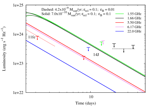
In Figure 2 we show models for $\epsilon_{\rm B}=0.01$ and 0.1. An almost perfect overlap between modeled light curves occurs for the combination $\dot{M}=7.0\times 10^{-10}\mbox{\,${\rm M_{\odot}\,yr^{-1}}$}$ and $\epsilon_{\rm B}=0.1$, and $\dot{M}=4.2\times 10^{-9}\mbox{\,${\rm M_{\odot}\,yr^{-1}}$}$and $\epsilon_{\rm B}=0.01$. Only at very early epochs ($\!\!\!\phantom{\leq}\smash{\buildrel\over{\lower 2.67502pt\hbox{$\buildrel\lower 2.14001pt\hbox{$\displaystyle<$}\over{\sim}$}}}\,\,3$ days after explosion), does SSA play a role for the lowest frequencies. The overlap is not surprising, since Equation 5 shows that $\dot{M}/v_{w}\propto\epsilon_{\rm B}^{-0.78}$ for fixed luminosity at early epochs in the optically thin part in our model. We note that Chomiuk et al. (2012) obtain a slightly different power-law index, $-0.7$, in their model. For all models in Figure 2, $\gamma_{\rm min}>1$ for the time span shown. This means that Equation 5 describes all light curves well, except for the lowest frequencies at $t\!\!\!\phantom{\leq}\smash{\buildrel\over{\lower 2.67502pt\hbox{$\buildrel\lower 2.14001pt\hbox{$\displaystyle<$}\over{\sim}$}}}\,\,3$ days.

The values of $\dot{M}/v_{w}$ for SN 2014J in Figure 2 are chosen so that the 5.50 GHz light curves go through the JVLA 3$\sigma$ upper limit on day 8.2. The light curves for other frequencies lie below their corresponding upper limits. The second most constraining limit is from our 1.55 GHz eMERLIN observation on day 13.8, yielding $\dot{M}\!\!\!\phantom{\leq}\smash{\buildrel\over{\lower 2.67502pt\hbox{$\buildrel\lower 2.14001pt\hbox{$\displaystyle<$}\over{\sim}$}}}\,\,1.15~{}(7.0)\times 10^{-9}\mbox{\,${\rm M_{\odot}\,yr^{-1}}$}$ for $\epsilon_{\rm B}=0.1~{}(0.01)$ and $v_{w}=100~{}\mbox{\,km s${}^{-1}$}$. We show in Table 1 upper limits for all data points.

Figure 2 also includes the most constraining upper limit for SN 2011fe (Chomiuk et al., 2012), together with a 5.9 GHz light curve using $\dot{M}=5.0\times 10^{-10}\mbox{\,${\rm M_{\odot}\,yr^{-1}}$}$, $v_{w}=100~{}\mbox{\,km s${}^{-1}$}$ and $\epsilon_{\rm B}=0.1$. The limit on mass-loss rate is somewhat below that of Chomiuk et al. (2012), who obtained $6.0\times 10^{-10}\mbox{\,${\rm M_{\odot}\,yr^{-1}}$}(v_{w}/100~{}\mbox{\,km s${}^{-1}$})$. The difference in those values probably stems from the difference in shell thickness of the emitting region, where we have adopted $\Delta r/r_{s}=0.2$ vs. $\Delta r/r_{s}=0.1$ (Chomiuk et al., 2012), and our fixed $T_{\rm bright}$. In any case, the difference in the upper limit on $\dot{M}/v_{w}$ is much smaller than that due to the uncertainty in $\epsilon_{\rm B}$.

In principle, radio non-detections could also be due to SSA during the observed epochs. In this case, the observed frequency $\nu_{\rm obs}<\nu_{\rm abs}$, and from Equation 1 we find that the observed flux at $\nu_{\rm obs}$ is $\propto r_{s}^{2}(v_{\rm obs}^{5}/v_{\rm abs})^{1/2}$. The combination of $r_{s}^{2}v_{\rm abs}^{-1/2}$ is a weak function of $\dot{M}/v_{w}$, and to make SSA important for the observations discussed here would require values of $\dot{M}/v_{w}$ much larger than those at which free-free absorption becomes important. We can therefore fully dismiss SSA as a cause for the radio non-detections of SN 2014J.

Figure 3.— Same as in Figure 2, but for circumstellar gas with constant density ($s=0$), i.e., the insterstellar medium (ISM). Solid lines are for $n_{\rm ISM}=1.33\mbox{\,cm${}^{-3}$}$, and dashed line is for $n_{\rm ISM}=12\mbox{\,cm${}^{-3}$}$, assuming $\epsilon_{\rm B}=0.1$ and $\epsilon_{\rm B}=0.01$, respectively. The data upper limits for SN 2014J are the same as in Figure 2. The constraint on $n_{\rm ISM}$ is set by the stacked 1.66 GHz eEVN data from days 20 and 35. The change in spectral slope around 25 days for the $\epsilon_{\rm B}=0.01$ model is due to the $\gamma_{\rm min}\geq 1$ constraint then coming into effect. For a comparison we also show the 3$\sigma$ upper limit from the stacked 5.9 GHz sample for SN 2011fe between days $2.1-19.2$ (Chomiuk et al., 2012), together with part of the light curve for a model (dotted red line) assuming $n_{\rm ISM}=7.0\mbox{\,cm${}^{-3}$}$ and $\epsilon_{\rm B}=0.1$.

Figure 4.— Same as in Figure 2, but for different values of $p$ and $n$. The values of $\dot{M}/v_{w}$ were chosen for the 5.50 GHz light curve to cross the upper JVLA limit from day 8.2. Note the change in slopes for the dashed lines around day 9, when the condition $\gamma_{\rm min}\geq 1$ comes into effect. See text for further details.

4.1.2 The constant density case, $s=0$.

If the progenitor of SN 2014J followed the double-degenerate channel, then the exploding WD is expected to be surrounded by the interstellar medium (ISM), which has a constant density. Chomiuk et al. (2012) discussed this scenario for SN 2011fe, and obtained a limit for the density of $\!\!\!\phantom{\leq}\smash{\buildrel\over{\lower 2.67502pt\hbox{$\buildrel\lower 2.14001pt\hbox{$\displaystyle<$}\over{\sim}$}}}\,\,6\mbox{\,cm${}^{-3}$}$ ($\epsilon_{\rm B}=0.1$).

The general behavior of the radio light curves for the constant density ISM case is different from the $n_{\rm CSM}\propto r^{-2}$ wind case in §4.1.1. For the constant density case and $p=3$, the radio luminosity increases with time (see also Chomiuk et al., 2012) according to

$$L_{\nu,{\rm thin}}\propto T_{\rm bright}~{}\epsilon_{\rm rel}^{1.71}~{}\epsilon_{\rm B}^{1.07}~{}n_{\rm ISM}^{1.10}~{}t^{0.38},$$ (7)

if $\gamma_{\rm min}$ is not fixed. If it is fixed

$$L_{\nu,{\rm thin}}\propto T_{\rm bright}~{}\epsilon_{\rm rel}^{0.86}~{}\epsilon_{\rm B}^{1.07}~{}n_{\rm ISM}^{1.27}~{}t^{0.88}.$$ (8)

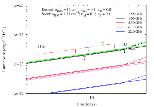
Here, we substituted $n_{\rm CSM}$ with $n_{\rm ISM}$ to highlight the likely origin of the gas in the $s=0$ case. Figure 3 shows models with densities $n_{\rm ISM}=1.33\mbox{\,cm${}^{-3}$}$ ($\epsilon_{\rm B}=0.1$) and $n_{\rm ISM}=12\mbox{\,cm${}^{-3}$}$ ($\epsilon_{\rm B}=0.01$). Scaling according to $n_{\rm ISM}\propto\epsilon_{\rm B}^{-0.97}$ (cf. Equation 7) makes the light curves for these models overlap fully, except for $t\!\!\!\phantom{\geq}\smash{\buildrel\over{\lower 2.67502pt\hbox{$\buildrel\lower 2.14001pt\hbox{$\displaystyle>$}\over{\sim}$}}}\,\,25$ days, when the condition $\gamma_{\rm min}\geq 1$ becomes important for the $n_{\rm ISM}=12\mbox{\,cm${}^{-3}$}$ model. The most constraining data are our eEVN 1.66 GHz data, stacked together, and the model parameters were chosen for the modeled radio luminosity to match those data. However, due to the $\gamma_{\rm min}\geq 1$ constraint, the 35 day data alone are almost as constraining as the stacked data.

In Figure 3, we also show the stacked 5.9 GHz data for SN 2011fe (Chomiuk et al., 2012), together with a model characterized by $n_{\rm ISM}=7.0\mbox{\,cm${}^{-3}$}$ and $\epsilon_{\rm B}=0.1$. We are thus close to Chomiuk et al. (2012) regarding the limit on $n_{\rm ISM}$ for SN 2011fe. For $s=0$, we used $\Delta r/r_{s}=0.12$, which is close to the value 0.1 used by Chomiuk et al. (2012). The limit on $n_{\rm ISM}$ we find for SN 2014J is $\approx 5.3$ times lower than for SN 2011fe, and is therefore clearly the lowest limit on density for the constant density case in any SN Ia.

As for the $s=2$ case, SSA is unimportant for the $s=0$ case. To be efficient enough to mute the radio emission to be consistent with the observed upper limit, $n_{\rm ISM}$ would have to be $\!\!\!\phantom{\geq}\smash{\buildrel\over{\lower 2.67502pt\hbox{$\buildrel\lower 2.14001pt\hbox{$\displaystyle>$}\over{\sim}$}}}\,\,10^{14}\mbox{\,cm${}^{-3}$}$ (for $\epsilon_{\rm B}\leq 0.1$), which is fully ruled out from X-ray limits, as well the normal optical behaviour of the supernova.

4.2. Sensitivity of results to parameters

While usually not acknowledged in the SN Ia literature, the obtained radio and X-ray upper limits on the circumstellar density are model dependent. In particular, Equations 5 through 8 show how most parameters influence the results.

We already mentioned the uncertainty in $\epsilon_{\rm rel}$ and, especially, $\epsilon_{\rm B}$, whereas $T_{\rm bright}$ is observationally constrained by other similar radio sources. The thickness of the radio-emitting region is yet another source of uncertainty, but probably small in comparison to other uncertainties.

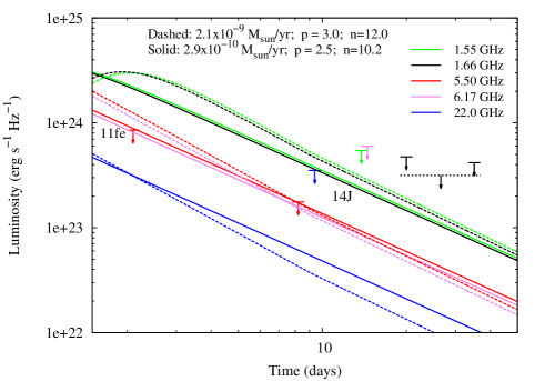
There is also an uncertainty in the upper limit on $\dot{M}/v_{w}$ due to values chosen for $n$ and $p$. Figure 4 shows two models, both with $\epsilon_{\rm B}=0.1$ and $\epsilon_{\rm rel}=0.1$, but where we have also assumed $p=2.5$ and $n=10.2$ (solid lines), and $p=3$ and $n=12$ (dashed lines). In both models we have used the earliest $3\sigma$ JVLA point for SN 2014J to constrain $\dot{M}/v_{w}$. For the $p=2.5$ model, $\dot{M}/v_{w}=2.9\times 10^{-10}\mbox{\,${\rm M_{\odot}\,yr^{-1}}$}$, i.e., a factor $\approx 2.4$ lower than the $p=3$ model in Figure 2. The choice of $p=3$ therefore gives a conservative limit on $\dot{M}/v_{w}$, unless $p>3$. Judging from Type Ib/Ic SNe, the expected deviation from $p=3$ is not large (Chevalier & Fransson, 2006), so we do not consider the uncertainty in $p$ being a major source of uncertainty for $\dot{M}/v_{w}$.

For the $n=12$ model, $\dot{M}/v_{w}=2.1\times 10^{-9}\mbox{\,${\rm M_{\odot}\,yr^{-1}}$}$, i.e., a factor $\approx 3.0$ higher than the $n=10.2$ model in Figure 2. The choice of $n=10.2$ may give too low a limit on $\dot{M}/v_{w}$, unless a shallower density profile than $n=10.2$ is expected. Indeed, Dwarkadas & Chevalier (1998) argue that an exponential density profile of the outer ejecta fits early explosion models better than a power law, and could indicate steeper profiles than at least $n=7$ for the outermost ejecta. We have also run models for $n=7$, but the value for $\dot{M}/v_{w}$ then becomes so low ($<10^{-11}\mbox{\,${\rm M_{\odot}\,yr^{-1}}$}$) that the model breaks down, producing shock velocities in excess of $c$. For such low wind densities, a relativistic treatment of the shock interaction is needed, similar to for gamma-ray bursts. From the models of Matzner & McKee (1999) it seems reasonable to assume that $n\!\!\!\phantom{\geq}\smash{\buildrel\over{\lower 2.67502pt\hbox{$\buildrel\lower 2.14001pt\hbox{$\displaystyle>$}\over{\sim}$}}}\,\,9$ for the outermost ejecta, which in our model would imply an upper limit of $\dot{M}/v_{w}\approx 2.0\times 10^{-10}\mbox{\,${\rm M_{\odot}\,yr^{-1}}$}$. The span in upper limit on $\dot{M}/v_{w}$ by a factor of $\approx 10.5$ between $9\leq n\leq 12$ shows that the unknown density profile for the outermost ejecta is an important source of uncertainty, and that accurate models for the outermost ejecta are needed. This is even more evident for the constant density case $s=0$, for which we find that our limit on $n_{\rm ISM}$ ranges from $\approx 0.17\mbox{\,cm${}^{-3}$}$ for $n=9$ to $\approx 6.3\mbox{\,cm${}^{-3}$}$ for $n=12$, assuming $\epsilon_{\rm B}=0.1$, $\epsilon_{\rm rel}=0.1$ and $p=3$. The solution for $n=9$ is, however, unphysical due to too large velocities for the shock during the first $\sim 10$ days, calling for a relativistic treatment of the dynamics.

5. Discussion

5.1. The possible progenitors of SN 2014J

5.1.1 Single Degenerate progenitor systems

The SD progenitor systems involve only one WD and include, in decreasing order of mass-loss rate from the supernova progenitor, symbiotic systems, WDs with steady nuclear burning, and recurrent novae.

In a symbiotic system, the WD accretes mass from a giant star (Hachisu et al., 1999). The WD loses this accreted matter at rates of $\dot{M}\gtrsim 10^{-8}$ ${\rm M_{\odot}\,yr^{-1}}$and $v_{w}\approx 30$ km s^-1. The radio emission from those systems should have been detected by our deep sensitive observations. Thus, our radio non-detection rules out a symbiotic system as the progenitor of SN 2014J (red region in Figure 5).

Another possible SD scenario is one where a main sequence, subgiant, helium, or giant star undergoes Roche lobe overflow onto the WD at rates of $3.1\times 10^{-7}\mbox{\,${\rm M_{\odot}\,yr^{-1}}$}\lesssim\dot{M}\lesssim 6.7\times 10^{-7}\mbox{\,${\rm M_{\odot}\,yr^{-1}}$}$ (Nomoto et al., 2007). At those accretion rates, the WD experiences steady nuclear burning (Shen & Bildsten, 2007). For an assumed fraction $\epsilon_{\rm loss}=0.01$ of the transferred mass to be lost from the system, the mass-loss rate is constrained to $3.1\times 10^{-9}~{}\mbox{\,${\rm M_{\odot}\,yr^{-1}}$}\lesssim\dot{M}\lesssim 6.7\times 10^{-9}~{}\mbox{\,${\rm M_{\odot}\,yr^{-1}}$}$ and typical speeds of 100  km s^-1$\lesssim v_{w}\lesssim$ 3000  km s^-1, where the low speeds apply for steady nuclear burning, while the high speeds apply to the systems with the highest accretion rates. At the lower end of $\dot{M}$, the mass loss through the outer Lagrangian points of the system proceeds at speeds up to $\sim$600  km s^-1. Most of the parameter space for the low-accretion rate scenario is ruled out by our radio observations, if $\epsilon_{\rm{\rm B}}\simeq 0.1$ (blue region in Fig. 5). At the upper end of $\dot{M}$ the winds become optically thick, limiting the accretion rate to $\dot{M}_{\rm acc}\approx 6\times 10^{-7}~{}M_{\odot}~{}\rm yr^{-1}$ and wind speeds of a few $\times$ 1000  km s^-1(Hachisu et al., 1999, 2008). Our data essentially rule out completely the high-accretion rate scenario of a WD with steady nuclear burning (cyan region in Fig. 5).

Finally, another possible SD channel is that of recurrent novae, which lie at the lowest accretion rate regime among popular SD scenarios. Here, a WD accreting at a rate $\dot{M}\approx(1-3)\times 10^{-7}~{}\mbox{\,${\rm M_{\odot}\,yr^{-1}}$}$, ejects shells of material at speeds of a few $\times 1000\mbox{\,km s${}^{-1}$}$, with typical recurrence times of a few years. The radio observations in Table 1 probe a radius of $\simeq(0.7-2.6)\times 10^{16}$ cm (for $s=2$ and $\epsilon_{\rm B}=0.1$), which constrains the presence of shells with recurrence times of $\lesssim 1.6~{}(v_{\rm shell}/2000~{}\mbox{\,km s${}^{-1}$})^{-1}\ (r_{\rm shell}/10^{16}\ {\rm cm})$ yr. Models of recurrent novae seem to indicate that as much as $\sim$15% of the accreted material over the recurrence time is ejected (Yaron et al., 2005; Shen & Bildsten, 2007). For the typical accretion rates above, this implies an ejected shell mass of $\approx(2.4-7.1)\times 10^{-8}\ (v_{\rm shell}/2000~{}\mbox{\,km s${}^{-1}$})^{-1}\ (r_{\rm shell}/10^{16}\ {\rm cm})~{}M_{\odot}$, which should have been detected by our sensitive observations (see gold region in Fig. 5). Unfortunately, the short duration of the nova radio burst, a few days at most, may have prevented its detection, so we cannot rule out completely the possibility of a nova shell ejection. During the quiescent phase between nova shell ejections, the WD accretes at a rate of $\dot{M}\sim 1\times 10^{-7}~{}\mbox{\,${\rm M_{\odot}\,yr^{-1}}$}$, so that the mass-loss wind parameter is $\dot{M}/v_{w}\sim 1\times 10^{-9}\ (\epsilon_{\rm loss}/0.01)/100$ km s^-1. If $\epsilon_{\rm B}=0.1$, our observations rule out almost completely the scenario with WD accretion during the quiescent phase of the star, whereas the case with $\epsilon_{\rm B}=0.01$ cannot be excluded completely (green region in Fig. 5).

In summary, our observations exclude completely symbiotic systems and the majority of the parameter space associated with stable nuclear burning WDs, as viable progenitor systems for SN 2014J. Recurrent novae with main sequence or subgiant donors cannot be ruled out completely, yet most of their parameter space is also excluded by our observations.

Figure 5.— Constraints on the parameter space (wind speed vs. mass-loss rate) for single degenerate scenarios for SN 2014J. The progenitor scenarios discussed in §5.1.1 are plotted as schematic zones, following Chomiuk et al. (2012). We indicate our 3$\sigma$ limits on $\dot{M}/v_{w}$, assuming $\epsilon_{\rm B}$ = 0.1 (solid; corresponding to the solid curves in Figure 2) and the conservative case of $\epsilon_{\rm B}$ = 0.01 (dashed; corresponding to the dashed curves in Figure 2). Mass loss scenarios falling into the gray shaded areas should have been detected by our deep radio observations, and therefore are ruled out for SN 2014J. Not included in the figure is the spun-up/spun-down progenitor scenario discussed in §5.2, as this predicts a constant density. For a comparison, we include our reassessed limit for SN 2011fe (dash-dotted line) for the same choice of parameters as the solid line for SN 2014J, which essentially leaves only room for quiescent nova emission as a viable alternative among the SD scenarios for SN 2011fe.

5.1.2 Double Degenerate progenitor systems

The alternative to a SD scenario is the DD channel, which involves two WDs in a binary system. In this case, the progenitor star is expected to have exploded in a constant ambient density medium. We can estimate the density in the region surrounding SN 2014J from the column density of neutral hydrogen toward the supernova position, $N_{\rm H\,I}\sim 2\times 10^{20}$ cm^-2 (Zwaan et al., 2008). Assuming a path length, $l\sim$ 100 pc, and solar abundance ($\mu\approx 1.4$), the particle number density at the supernova location is $\mu\,N_{\rm H\,I}/l\sim$ 0.9 cm^-3. Our stacked eEVN limits imply $n_{\rm ISM}\lesssim 1.3(12)$ cm^-3 for $\epsilon_{B}=0.1$ (0.01), and are thus consistent with the SN directly expanding into the interstellar medium. Therefore, our radio non-detections are consistent with the DD channel for SNe Ia.

We note that the limit imposed on $n_{\rm ISM}$ by the microphysical parameter $\epsilon_{\rm B}=0.1$ is formally similar to the likely value of $n_{\rm ISM}$ at the SN location. Yet, the uncertainties involved in this estimate are such that both values are in agreement. At any rate, the sensitivity of $\epsilon_{\rm B}$ on $n_{\rm ISM}$ demonstrates the usefulness of late-time radio observations to constrain this relevant microphysical parameter in SNe Ia. For example, a non-detection of SN 2014J one year after explosion with the same observational limit as from our stacked 1.66 GHz observations would, according to our model, constrain $n_{\rm ISM}$ to $\!\!\!\phantom{\leq}\smash{\buildrel\over{\lower 2.67502pt\hbox{$\buildrel\lower 2.14001pt\hbox{$\displaystyle<$}\over{\sim}$}}}\,\,0.27\mbox{\,cm${}^{-3}$}$, assuming $\epsilon_{\rm{\rm B}}=0.1$, $\epsilon_{\rm rel}=0.1$, $n=10.2$, $p=3$ and $\gamma_{\rm min}=1$. The supernova shock wave will at this point be located at $r_{s}\approx 1.6\times 10^{17}$ cm. A non-detection at such late epochs and such low flux levels, will certainly be very useful in constraining $\epsilon_{\rm B}$.

5.2. Broader picture

The recent and nearby SNe 2011fe and 2014J have offered a remarkable possibility to learn about the origin of SNe Ia. We have shown here that deep radio observations can be used to rule out several progenitor models for SN 2014J  and a similar discussion was made for SN 2011fe by Chomiuk et al. (2012). In addition to this, Margutti et al. (2012) provided deep limits for SN 2011fe from X-rays (cf. §1), which do not depend on $\epsilon_{\rm B}$, but where the limit on circumstellar density has a stronger dependence on $\epsilon_{\rm rel}$ and $\gamma_{\rm min}$ than for radio emission. While $\epsilon_{\rm rel}=0.1$ has been used by us and others, it must be cautioned that, e.g., SN 1993J had a much lower value (Fransson & Björnsson, 1998; Pérez-Torres et al., 2001; Martí-Vidal et al., 2011), although it is clear that this supernova bears little resemblance with Type Ib/Ic SNe, which have been used as templates to model SNe Ia.

For SN 2011fe, the non-detections in radio and X-rays were accompanied with no circumstellar line absorption (Patat et al., 2013) and a non-detection of late nebular emission from gas ablated off an SD companion (Shappee, 2013b). This, together with other evidence for SN 2011fe (see Maoz et al., 2014), has been used to argue for an increased likelihood of SNe Ia being the endpoint of a DD scenario rather than SD scenarios. Our non-detections of radio emission from SN 2014J in principle add to this evidence.

However, Justham (2011) suggested that a SD scenario, with a spun-up/spun-down super-Chandrasekhar WD (see also Di Stefano et al., 2011; Hachisu et al., 2012), can still be possible if the donor star shrinks far inside its Roche lobe prior to the explosion. This would make the SD companion smaller and more tightly bound, and only very dilute circumstellar gas would be expected in the immediate vicinity of the WD. Di Stefano et al. (2011) argue that density could be of the same order as typical interstellar densities. Continued radio observations of both SNe 2011fe and 2014J could be useful to test the presence of such low-density gas (cf. §5.1.2).

For a typical time-scale of $\sim 10^{3}$ years between last Roche-lobe overflow and explosion (Justham, 2011), and a wind speed of $100\mbox{\,km s${}^{-1}$}$, the last traces of substantial circumstellar gas could in this scenario be at a distance of $\sim 3\times 10^{17}$ cm, and could explain the presumed shell around, e.g., SN 2006X (Patat et al., 2007). If the supernova ejecta would start to interact with such a shell, radio emission would increase. Radio observations of SN 2006X (Chandra et al., 2008) two years after explosion, however, failed to detect any emission. Patat et al. (2007) estimated a shell radius of $\sim 10^{16}$ cm, which according to the estimate in §5.1.1, was most likely overtaken by the supernova ejecta by $t\approx 2$ years. Continued monitoring of SN 2014J would be useful to trace these putative shells.

We emphasize that shells around supernovae do not have to lie along the line of sight to be detected in radio, as opposed to the narrow absorption line features. This should increase the possibility to detect such shells in the radio, especially if shells are as common as suggested (see §2). Interaction with shells are also better observed in the radio than in X-rays, as no inverse Compton scattering is expected at late times when the supernova has faded and the distance from the line emitting SN ejecta and the shell is large.

Shappee (2013a) caution that the lack of signatures from an SD companion could be a problem for the model of Justham (2011), as only $\!\!\!\phantom{\leq}\smash{\buildrel\over{\lower 2.67502pt\hbox{$\buildrel\lower 2.14001pt\hbox{$\displaystyle<$}\over{\sim}$}}}\,\,0.001~{}\hbox{M${}_{\odot}$}$ of ablated mass from the companion can be accommodated by the observations of Shappee (2013b), in combination with an extrapolation of the models presented in Mattila et al. (2005) and Lundqvist et al. (2013), before giving rise to detectable H$\alpha$ emission in the nebular phase; all models calculated by Marietta et al. (2000), Pan et al. (2012) and Liu et al. (2012) predict more than $\sim 0.01~{}\hbox{M${}_{\odot}$}$ of ablated mass. A way to avoid H$\alpha$ emission is, of course, if the donor is He-rich. The models of Liu et al. (2013) show that of order $\sim 0.02~{}\hbox{M${}_{\odot}$}$ of He-rich gas would then reside in the centre of the supernova in the nebular phase. However, even if the donor is H-rich, the caution by Shappee (2013a) should not be over interpreted.

The opacity in the nebular emission models of Mattila et al. (2005) and Lundqvist et al. (2013) does not contain as many spectral lines as more recent models by, e.g., Jerkstrand et al. (2011). Scattering in the spectral region around H$\alpha$ could be more severe than previously anticipated, and the constraint from lack of nebular H$\alpha$ less important. Nebular lines further out in the red should suffer from less scattering, and the models discussed in Lundqvist et al. (2013) show that narrow ($\!\!\!\phantom{\leq}\smash{\buildrel\over{\lower 2.67502pt\hbox{$\buildrel\lower 2.14001pt\hbox{$\displaystyle<$}\over{\sim}$}}}\,\,10^{3}\mbox{\,km s${}^{-1}$}$) [Ca II] lines are present in the red, and could thus be more constraining than H$\alpha$. Traces of these lines could be useful to test scenarios with both H- and He-rich donors. Further detailed modeling of the nebular phase is indeed needed, as well as modeling of supernova ejecta colliding with compact companions such as those in the models of Justham (2011).

Deep nebular spectra of SN 2014J are warranted to test those impact models, due to the SN proximity. A potential problem is, however, the extinction toward SN 2014J and the complicated interstellar imprint on the supernova spectrum (Goobar et al., 2014; Welty et al., 2014). The latter may, in particular, make the search for narrow-line variations more cumbersome than for, e.g., SN 2006X.

5.3. Future outlook for radio observations of SNe Ia

At the moment, our deepest radio limits on circumstellar gas are for SNe 2011fe and 2014J. With the advent of the Square Kilometre Array (SKA), we will be able to obtain significantly deeper radio limits (or, potentially, a detection) for SNe Ia exploding at the distance of M 82. For more distant supernovae, we will obtain similar limits to those obtained for SNe 2011fe and 2014J, which will allow us to build a picture from a larger statistical sample.

The first phase of SKA considers three different components. One of them, SKA1-mid, promises to yield 1$\sigma$ sensitivities of $\sim 0.7\mu$Jy/b in one hour at a fiducial frequency of 1.7 GHz. This figure is five times better than currently provided by the most sensitive array, the JVLA. Therefore, SKA1-mid should be able to either detect the putative radio emission of SN 2014J-like objects up to distances $\lesssim 8$ Mpc in less than one hour, or put significantly better constraints on some of the parameter space of SD scenarios for the next SN Ia that explodes in M 82, some of which could not be completely ruled out even by our very deep radio observations. However, the expected number of SN Ia per year in such a volume of the local universe is small. Indeed, since the volumetric SN Ia rate is $\sim 3\times 10^{-5}$ SN/yr/Mpc^-3 (Dilday et al., 2010), we should expect on average one SN Ia every $\sim$15 yr within a distance of $\!\!\!\phantom{\leq}\smash{\buildrel\over{\lower 2.67502pt\hbox{$\buildrel\lower 2.14001pt\hbox{$\displaystyle<$}\over{\sim}$}}}\,\,$8 Mpc, which is a small value. To obtain a statistically significant sample of SNe Ia observed in radio, with similar upper limits to those obtained by us for SN 2014J, we need to sample significantly larger volumes and need much more sensitive radio observations. For example, by sampling out to a distance of 25 Mpc, we can expect $\sim$2 SNe Ia per year within the sampled volume, which in 10 years would result in a total of $\sim$20 SNe Ia, enough to extract statistical results. At this maximum distance, we need a sensitivity of $\sim$50 times better than obtained by the observations discussed here, to be as constraining, or $\sim 80$ nJy/b. When SKA is completed, the fiducial 1$\sigma$ sensitivity should be 10 times better than for SKA1-mid, or about $\sim 70$ nJy/b in one hour, and such statistical studies will be perfectly possible in short amounts of time. At this level of sensitivity, a non-detection would be essentially as meaningful as a direct detection, since the former would imply that only the DD scenario is viable, while the latter would tell us which of the SD channels result in SNe Ia.

6. Summary

We report deep eEVN and eMERLIN radio observations of the Type Ia SN 2014J in the nearby galaxy M 82, along with a detailed modeling of its radio emission. Our observations result in non-detections of the radio emission from SN 2014J. Yet, radio data and modeling allow us to place a tight constraint on the mass loss rate from the progenitor system of SN 2014J. Namely, if the exploding WD was surrounded by a wind with a density profile $\rho\propto r^{-2}$, as expected for a SD scenario, then our upper limit to the mass-loss rate is $\dot{M}\lesssim 7.0\times 10^{-10}~{}\mbox{\,${\rm M_{\odot}\,yr^{-1}}$}$, for a wind speed of $100\mbox{\,km s${}^{-1}$}$.

If, on the contrary, the circumstellar gas has a constant density, as expected to be the case for the DD scenario (but also in a small region of the parameter space of SD scenarios), then our modeling yields an upper limit on the gas density, such that $n_{\rm ISM}\lesssim 1.3\mbox{\,cm${}^{-3}$}$.

Our stringent upper limits to the circumstellar density around SN 2014J allow us to exclude completely symbiotic systems and the majority of the parameter space associated with stable nuclear burning WDs, as viable progenitor systems for SN 2014J. For the case of recurrent novae with main sequence or subgiant donors, we cannot rule out them completely, yet most of their parameter space is also excluded by our observations for the standard assumption of $\epsilon_{\rm B}=0.1$, where $\epsilon_{\rm B}$ is the ratio of magnetic energy density to post-shock thermal energy density.

We have also reassessed the radio limits on wind density for SN 2011fe, and for $\epsilon_{\rm B}=0.1$ we obtain $\dot{M}\lesssim 5.0\times 10^{-10}~{}\mbox{\,${\rm M_{\odot}\,yr^{-1}}$}$ (for a wind speed of $100\mbox{\,km s${}^{-1}$}$) and $n_{\rm ISM}\lesssim 7.0\mbox{\,cm${}^{-3}$}$. These limits are close to those calculated by Chomiuk et al. (2012). Our limit on $\dot{M}/v_{w}$ for SN 2014J is thus similar to that for SN 2011fe, whereas for the constant density case we obtain a much lower limit than for SN 2011fe, and hence the lowest limit for a constant density ambient around a SN Ia.

The combined radio limits on circumstellar gas around SNe 2011fe and 2014J add to evidence from mainly non-detections of X-rays from SN 2011fe and 2014J(Margutti et al., 2012; mar14) and no detection of H$\alpha$ in the nebular phase of SN 2011fe (Shappee, 2013b), that SNe Ia are very likely to stem from the DD scenario, rather than SD scenarios.

Finally, we highlight future observations with the Square Kilometre Array (SKA). When fully completed, the SKA is likely to yield limits on circumstellar gas for future SNe Ia similar to the limits reported here for the nearby SNe 2011fe and 2014J, but for distances well beyond the Virgo cluster. For nearby SNe Ia, SKA limits are likely to be fully conclusive regarding the origin of the progenitor systems of SNe Ia.

References

- Björnsson & Lundqvist (2014) Björnsson, C.-I., & Lundqvist, P. 2014, ApJ, 787, 143
- Branch et al. (1995) Branch, D., Livio, M., Yungelson, L. R., Boffi, F. R., & Baron, E. 1995, PASP, 107, 1019
- Cao et al. (2014) Cao, Y., Kasliwal, M. M., McKay, A., & Bradley, A. 2014, ATel, 5786, 1
- Chandler & Marvil (2014) Chandler, C. J., & Marvil, J. 2014, ATel, 5812
- Chandra et al. (2008) Chandra, P., Chevalier, R., & Patat, P. 2008, ATel, 1391, 1
- Chevalier (1982a) Chevalier, R. A. 1982a, ApJ, 258, 790
- Chevalier (1982b) Chevalier, R. A. 1982b, ApJ, 259, 302
- Chevalier (1998) Chevalier, R. A. 1998, ApJ, 499, 810
- Chevalier & Fransson (2006) Chevalier, R. A., & Fransson 2006, ApJ, 651, 381
- Chomiuk et al. (2012) Chomiuk, L., Soderberg, A. M., Moe, M., et al. 2012, ApJ, 750, 164
- Chugai (2008) Chugai, N. N. 2008, Astronomy Letters, 34, 389
- Chugai et al. (2004) Chugai, N. N., Chevalier, R. A., & Lundqvist, P. 2004, MNRAS, 355, 627
- Cumming et al. (1996) Cumming, R. J., Lundqvist, P., Smith, L. J., Pettini, M., & King, D. L. 1996, MNRAS, 283, 1355
- Dilday et al. (2010) Dilday, B., Smith, M., Bassett, B., et al. 2010, ApJ, 713, 1026
- Dilday et al. (2012) Dilday, B., Howell, D. A., Cenko, S. B., et al. 2012, Science, 337, 942
- Di Stefano et al. (2011) Di Stefano, R., Voss, R., & Clayes, J. S. W. 2011, ApJ, 738, L1
- Dwarkadas & Chevalier (1998) Dwarkadas, V. V., & Chevalier, R. A. 1998, ApJ, 497, 807
- Fink et al. (2014) Fink, M., Kromer, M., Seitenzahl, I. R., et al. 2014, MNRAS, 438, 1762
- Fossey et al. (2014) Fossey, J., Cooke, B., Pollack, G., Wilde, M., & Wright, T. 2014, CBET, 3792, 2
- Fransson & Björnsson (1998) Fransson, C., & Björnsson, C.-I. 1998, ApJ, 509, 861
- Goobar et al. (2014) Goobar, A., Johansson, J., Amanullah, R., et al. 2014, ApJ, 784, L12
- Hachisu et al. (1999) Hachisu, I., Kato, M., & Nomoto, K. 1999, ApJ, 522, 487
- Hachisu et al. (2008) Hachisu, I., Kato, M., & Nomoto, K. 2008, ApJ, 679, 1390
- Hachisu et al. (2012) Hachisu, I., Kato, M., Saio, H., & Nomoto, K. 2012, ApJ, 744, 69
- Hancock et al. (2011) Hancock, P. J., Gaensler, B. M., & Murphy, T. 2011, ApJ, 735, 35
- Horesh et al. (2011) Horesh, A., Kulkarni, S. R., Fox, D. B., et al. 2012, ApJ, 746, 21
- Hughes et al. (2007) Hughes, J. P., Chugai, N., Chevalier, R., Lundqvist, P., & Schlegel, E. 2007, ApJ, 670, 1260
- Itagaki et al. (2014) Itagaki, K., Kaneda, H., Yamaoka, H., et al. 2014, CBET, 3792, 1
- Jerkstrand et al. (2011) Jerkstrand, A., Fransson, C., & Kozma, C. 2011, A&A, 535, 45
- Justham (2011) Justham, S. 2011, ApJ, 730, L34
- Liu et al. (2012) Liu, Z. W., Pakmor, R., Röpke, F. K., et al. 2012, A&A, 548, A2
- Liu et al. (2013) Liu, Z. W., Pakmor, R., Seitenzahl, I. R., et al. 2013, ApJ, 774, 37
- Lundqvist & Fransson (1988) Lundqvist, P., & Fransson, C. 1988, A&A, 192, 221
- Lundqvist et al. (2013) Lundqvist, P., Mattila, S., Sollerman, J., et al. 2013, MNRAS, 435, 329
- Maoz et al. (2014) Maoz, D., Mannucci, F., & Nelemans, G. 2014, ARA&A, in press; arXiv1312.628M
- Margutti et al. (2014) Margutti, R., Parrent, J., Kamble, A., et al. 2014, ApJ, submitted, arXiv:1405.1488
- Margutti et al. (2012) Margutti, R., Soderberg, A. M., Chomiuk, L., et al. 2012, ApJ, 751, 134
- Marietta et al. (2000) Marietta, E., Burrows, A., & Fryxell, B. 2000, ApJS, 128, 615
- Martí-Vidal et al. (2011) Martí-Vidal, I., Marcaide, J. M., Alberdi, A., et al. 2011, A&A, 526, A143
- Mattila et al. (2005) Mattila, S., Lundqvist, P., Sollerman, J., et al. 2005, A&A, 443, 649
- Matzner & McKee (1999) Matzner, C.D., & McKee, C.F., ApJ, 510, 379
- Nomoto et al. (2007) Nomoto, K., Saio, H., Kato, M., & Hachisu, I. 2007, ApJ, 663, 1269
- Pan et al. (2012) Pan, K.-C., Ricker, P. M., & Taam, R. E. 2012, ApJ, 750, 151
- Panagia et al. (2006) Panagia, N., Van Dyk, S. D., Weiler, K. W., et al. 2006, ApJ, 646, 369
- Patat et al. (2007) Patat, N., Chandra, P., Chevalier, R., et al. 2007, Science, 317, 924
- Patat et al. (2013) Patat, N., Cordiner, M. A., Cox, N. L. J., et al. 2013, A&A, 549, 62
- Pérez-Torres et al. (2001) Pérez-Torres, M. A., Alberdi, A., & Marcaide, J. M. 2001, A&A, 374, 997
- Perlmutter et al. (1999) Perlmutter, S., Aldering, G., Goldhaber, G., et al. 1999, ApJ, 517, 565
- Readhead (1994) Readhead, A. C. S. 1994, ApJ, 426, 51
- Riess et al. (1998) Riess, A., Filippenko, A. V., Challis, P., et al., 1998, AJ, 116, 1009
- Rybicki & Lightman (1979) Rybicki, G. B., & Lightman, A. P. 1979, Radiative Processes in Astrophysics (New York: Wiley)
- Russell & Immler (2012) Russell, B. R., & Immler, S. 2012, ApJ, 748, L29
- Shappee (2013a) Shappee, B. J., Kochanek, C. S., & Stanek, K. Z. 2013a, ApJ, 765, 150
- Shappee (2013b) Shappee, B. J., Stanek, K. Z., Pogge, R. W., & Garnavich, P. M. 2013b, ApJ, 762, L5
- Shen & Bildsten (2007) Shen, K. J., & Bildsten, L. 2007, ApJ, 660, 1444
- Shen & Bildsten (2007) Shen, K. J., & Bildsten, L. 2009, ApJ, 692, 324
- Simon et al. (2009) Simon, J. D., Gal-Yam, A., Gnat, O., et al. 2009, ApJ, 702, 1157
- Smith et al. (2014) Smith, L. J., Strolger, L., Mutchler, M., Ubeda, L., & Levay, K. 2014, ATel, 5821, 1
- Soaker (2014) Soaker, N. 2014, arXiv:1405.0173
- Sternberg et al. (2014) Sternberg, A., Gal-Yam, A., Simon, J. D., et al. 2014, MNRAS, submitted, arXiv:1311.3645S
- Truelove & McKee (1999) Truelove, J. K., & McKee, C. E. ApJS, 120, 299
- Welty et al. (2014) Welty, D. E., Ritchey, A. M., Dahlstrom, J. A., & York, D. G. 2014, ApJ, submitted, arXiv:1404.2639
- Yaron et al. (2005) Yaron, O., Prialnik, D., Shara, M. M., & Kovetz, A. ApJ, 623, 398
- Zheng et al. (2014) Zheng, W., Shivvers, I., Filippenko, A. V., et al. 2014, ApJ, 783, L24
- Zwaan et al. (2008) Zwaan, M., Walter, F., Ryan-Weber, E., et al. 2008, AJ, 136, 2886