Josephson effect in normal and ferromagnetic topological insulator planar, step and edge junctions

Abstract

We investigate Josephson junctions on the surface of a three-dimensional topological insulator in planar, step, and edge geometries. The elliptical nature of the Dirac cone representing the side surface states of the topological insulator results in a scaling factor in the Josephson current in a step junction as compared to the planar junction. In edge junctions, the contribution of the Andreev bound states to the Josephson current vanishes due to spin-momentum locking of the surface states. Furthermore, we consider a junction with a ferromagnetic insulator between the superconducting regions. In these ferromagnetic junctions, we find an anomalous finite Josephson current at zero phase difference if the magnetization is pointing along the junction (and perpendicular to the Josephson current). An out-of-plane magnetization with respect to the central region of the junction opens up an exchange gap and leads to a non-monotonic behavior of the critical Josephson current for sufficiently large magnetization as the chemical potential increases.

I Introduction

Topological insulators are states of quantum matter whose electronic structure cannot be adiabatically connected to conventional insulators and semiconductors. They are characterized by an insulating gap in the bulk and gapless edge states (in case of a two-dimensional (2D) topological insulator) or surface states (in case of a three-dimensional (3D) system) which are protected by time-reversal (TR) symmetry against disorder and other perturbations that respect TR symmetry.Kane and Mele (2005a, b); Fu et al. (2007); Moore and Balents (2007); Roy (2009); Hasan and Kane (2010); Qi and Zhang (2011) The theoretical prediction of symmetry-protected edge states in HgTe quantum wellsBernevig et al. (2006) led to the experimental demonstration of HgTe quantum wells being 2D topological insulators.König et al. (2007) Similarly, the theoretical prediction of Bi_1-xSb_x being a 3D topological insulatorFu and Kane (2007) soon led to the experimental demonstration of 2D topological surface states in Bi_0.9Sb_0.1.Hsieh et al. (2008) More compounds were predicted to be 3D topological insulators using first-principles electronic structure calculations, which include Sb₂Te₃, Bi₂Te₃ and Bi₂Se₃.Zhang et al. (2009a) The surface states of these topological insulators were identified using angle-resolved photo-emission spectroscopyXia et al. (2009); Hsieh et al. (2009); Chen et al. (2009) and scanning tunneling microscopy.Zhang et al. (2009b); Alpichshev et al. (2010)

In this article we consider 3D topological insulators with symmetry protected 2D surface states. A simple low-energy effective model can be shown to describe the topological insulators Bi₂Se₃, Bi₂Te₃, and Sb₂Te₃ with a single Dirac cone on the surface.Zhang et al. (2009a) The topological insulator Bi₂Se₃ exhibits a circular Dirac cone on the surface perpendicular to the three-fold rotation symmetry axis (which we will call the top surface), and an elliptical Dirac cone on the side surfaces.Zhang et al. (2012); Alos-Palop et al. (2013) In the case of Bi₂Se₃, this ellipticity suppresses the conductance in a nanostep junction.Alos-Palop et al. (2013)

Recently, the consequences of induced superconductivityStanescu et al. (2010); Wang et al. (2012) and ferromagnetism at the surface of topological insulators have attracted a great deal of attention. In Refs. [Linder et al., 2010; Tanaka et al., 2009] transport properties of planar topological ferromagnetic junctions were studied. The authors calculated the Josephson current of such superconducting–ferromagnetic–superconducting (SFS) junctions and found an anomalous current-phase relation for a magnetization pointing in the direction of transport. This magnetization leads to a shift of the phase difference in the Josephson junction, such that a finite Josephson current is possible even at a phase difference $\phi=0$. The study in Refs. [Linder et al., 2010; Tanaka et al., 2009] is based on a Dirac-type surface Hamiltonian

$$H_{\rm Dirac}=\hbar v_{F}\left(\sigma_{x}k_{x}+\sigma_{y}k_{y}\right),$$ (1)

where $v_{F}$ denotes the Fermi velocity.

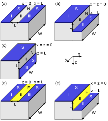
Figure 1: (Color online) (a) Planar, (b) step and (c) edge topological insulator junction and ferromagnetic (d) planar and (e) step junction. The S-planes are the superconductors inducing an effective p-wave superconductivity in the surface of the topological insulator (regions I and III). The weak link (i.e., the central region) of the junction in (a), (b) and (c) is the pristine normal-conducting (N) surface of the topological insulator (region II). In (d) and (e), region II is covered by a ferromagnetic insulator with magnetization $\mathbf{M}$ that induces an exchange coupling in the surface states.

In the present manuscript we investigate the impact of the elliptical nature of the Dirac cone on the proximity induced superconductivity in the surface states of a 3D topological insulator. We quantify our study by calculating the Josephson effect in superconducting–normal–superconducting (SNS) and SFS junctions on the surface of a 3D topological insulator involving two different side surfaces. We show that by measuring the critical current of these junctions, we can quantify the ellipticity of the Dirac cone, providing information about the bulk band structure and symmetry properties of these topological insulators. For concreteness, we use the effective low-energy model of the topological insulator Bi₂Se₃. First, we analyze the influence of the ellipticity of the Dirac cone on the different surfaces by evaluating the Josephson current in SNS planar, step and edge junctions as shown in Fig. 1 (a), (b) and (c). Afterwards, we calculate the Josephson effect in the SFS planar and step junctions shown in Fig. 1 (d) and (e), and analyze the dependence of the Josephson current on the direction of magnetization. Our results complement those of Refs. [Linder et al., 2010; Tanaka et al., 2009] because the surface states of the Bi₂Se₃ topological insulator are governed by a Rashba-type Hamiltonian of the form

$$H_{\rm Rashba}=\hbar v_{F}\left(\sigma_{x}k_{y}-\sigma_{y}k_{x}\right),$$ (2)

in contrast to the Dirac Hamiltonian shown in Eq. (1).

II Model

II.1 Hamiltonians and wave functions

Our goal is to calculate the Josephson effect for SNS planar, step and edge junctions and SFS planar and step junctions. The calculations are done for the 3D topological insulator Bi₂Se₃ and can be adapted to any topological insulator whose surface states are described by a Rashba-type Hamiltonian. The effective low-energy Hamiltonian for Bi₂Se₃ in the basis of four hybridized states of Se and Bi $p_{z}-$orbitals denoted as $|\,P1^{+}_{z}\uparrow\rangle$, $|\,P2^{-}_{z}\uparrow\rangle$, $|\,P1^{+}_{z}\downarrow\rangle$, $|\,P2^{-}_{z}\downarrow\rangle$ can be written as Zhang et al. (2009a)

$$H(\mathbf{k})=\varepsilon_{0}(\mathbf{k})\mathbb{I}_{4\times 4}+\begin{pmatrix}M(\mathbf{k})&A_{1}k_{z}&0&A_{2}k_{-}\\ A_{1}k_{z}&-M(\mathbf{k})&A_{2}k_{-}&0\\ 0&A_{2}k_{+}&M(\mathbf{k})&-A_{1}k_{z}\\ A_{2}k_{+}&0&-A_{1}k_{z}&-M(\mathbf{k})\end{pmatrix},$$ (3)

where $k_{\pm}=k_{x}\pm ik_{y}$, $\varepsilon_{0}(\mathbf{k})=C+D_{1}k_{z}^{2}+D_{2}k_{+}k_{-}$, $M(\mathbf{k})=M-B_{1}k_{z}^{2}-B_{2}k_{+}k_{-}$, and $k_{+}k_{-}=k_{x}^{2}+k_{y}^{2}$. The parameters $A_{1},A_{2},B_{1},B_{2},C,D_{1},D_{2},$ and $M$ can be determined by fitting the energy spectrum of this effective Hamiltonian with that of the ab initio calculations, see Ref. [Zhang et al., 2009a]. In the basis states, $\uparrow$ ($\downarrow$) stands for spin up (down) and $+$ ($-$) stands for even (odd) parity. There exists a straightforward procedure to obtain the effective Hamiltonian describing the surface states.Qi and Zhang (2011) The effective surface Hamiltonian for the $x-y$ plane of the topological insulator is then given by Qi and Zhang (2011); Fu (2009)

$$H^{xy}=\varepsilon_{0}^{xy}+\hbar v_{F}^{xy}(\sigma_{x}k_{y}-\sigma_{y}k_{x}),$$ (4)

where $\varepsilon_{0}^{xy}=C+(D_{1}/B_{1})M$ is the Dirac point energy, $v_{F}^{xy}=A_{2}\sqrt{1-(D_{1}/B_{1})^{2}}/\hbar$ represents the Fermi velocity in the $x-y$ plane, and $\sigma_{x,y,z}$ denote the Pauli matrices.

In contrast, the $y-z$ plane is described by the surface Hamiltonian

$$H^{yz}=\varepsilon_{0}^{yz}+\hbar v_{F}^{yz}(\sigma_{y}\eta k_{z}-\sigma_{z}k_{y}),$$ (5)

with the Dirac point energy $\varepsilon_{0}^{yz}=C+(D_{2}/B_{2})M$ and the Fermi velocity $v_{F}^{yz}=A_{2}\sqrt{1-(D_{2}/B_{2})^{2}}/\hbar$. The prefactor $\eta:=A_{1}/A_{2}$ in front of $k_{z}$ in $H^{yz}$ is a manifestation of the elliptical Dirac cone of the $y-z$ surface. This prefactor implies that the Fermi velocity in $z$ direction is different from the Fermi velocity in $y$ direction. On the $x-y$ surface, on the other hand, the Dirac cone is circular and the Fermi velocities in $x$ and $y$ directions are identical.

Since superconductivity couples the electron and hole wave functions, we write the surface states in the Nambu basis $\Psi=(\psi_{\uparrow},\psi_{\downarrow},\psi^{\dagger}_{\downarrow},-\psi^{\dagger}_{\uparrow})^{T}$. The Hamiltonian for the surface states is given by

$$\mathbf{H_{p}}=\begin{pmatrix}H^{p}-\mu+U+\mathbf{M}&\Delta_{0}e^{i\phi}\\ \Delta_{0}e^{-i\phi}&-H^{p}+\mu-U+\mathbf{M}\end{pmatrix},$$ (6)

where $H^{p}(\varepsilon_{0}^{p},v_{F}^{p})$ for $p=xy,yz$ denotes the respective surface Hamiltonian, $\mu$ the chemical potential, $U$ the electrostatic potential, $\Delta_{0}$ the induced superconducting pairing gap, $\phi$ the superconducting phase, and $\mathbf{M}=\mathbf{m}\cdot\boldsymbol{\sigma}$, where $\mathbf{m}=(m_{x},m_{y},m_{z})$ denotes an induced exchange field.

Figures 1(a), (b) and (c) show the geometries of the SNS junctions that we study. They are divided into three regions: regions I and III denote topological insulator surfaces with induced superconductivity, whereas region II denotes a normal conducting topological insulator surface (the weak link). The superconducting planes are produced by bringing the surface in contact with an $s$-wave superconductor. The proximity effect then induces effective $p$-wave superconductivity in the surface states.Fu and Kane (2008) It is assumed that there is an electrostatic potential $U$ in the three regions which can be adjusted independently by a gate voltage or doping. $U$ is measured from the chemical potential in region II. The low energy states in region II are thus described by Eq. (6) with $U=\Delta_{0}=\mathbf{M}=0$. In the superconducting regions I and III the potential is $U=-U_{0}$. Furthermore, in the superconducting regions we have $\Delta_{0}\neq 0$ and $\mathbf{M}=0$.

Figures 1 (d) and (e) show the SFS junctions. The ferromagnetic region II is established by placing a ferromagnetic insulator on top of the topological insulator, which induces an effective exchange coupling due to proximity effect.Tanaka et al. (2009) Consequently, the ferromagnetic region is described by Eq. (6) with $\mathbf{M}\neq 0$ and $U=0$.

We obtain $\Psi$ by solving the Bogoliubov-de-Gennes (BdG) equations $\mathbf{H_{p}}\Psi=\varepsilon\Psi$. The wave functions in the superconducting regions are calculated in a regime where $U_{0}\gg|\mu-\varepsilon_{0}^{p}|,\varepsilon$. This means that the Fermi wave length $\lambda^{\prime p}_{F}$ in the superconductor is small, i.e., $\lambda^{\prime p}_{F}\ll\lambda_{F}^{p},\xi$, where $\lambda_{F}^{p}=\hbar v_{F}^{p}/\mu$ is the Fermi wave length in the normal topological insulator surface and $\xi=\hbar v_{F}^{p}/\Delta_{0}$ is the superconducting coherence length. We only consider excitation energies smaller than the gap, $\varepsilon<\Delta_{0}$, which implies that we only evaluate the Josephson current due to Andreev bound states. Consequently, the momentum in $y$ direction fulfills $|k_{y}|\leq|(\mu-\varepsilon_{0}^{p})/\hbar v_{F}^{p}|$, which allows us to simplify the wave functions. Furthermore, we assume $U_{0}+\mu-\varepsilon_{0}^{p}\gg\Delta_{0},\varepsilon$. Then, the surface states in region I of all the junctions considered in this manuscript are described by

$$\Psi_{all,S}^{I\pm}(x,y) =(e^{\mp i\beta},\mp ie^{\mp i\beta},e^{-i\phi_{I}},\mp ie^{-i\phi_{I}})^{T}e^{ik_{y}y\pm ik_{x}x+\kappa x},$$ (7)

where

$$\beta =\arccos(\varepsilon/\Delta_{0})\>,$$

$$k_{x} =\sqrt{\frac{(U_{0}+\mu-\varepsilon_{0}^{xy})^{2}}{(\hbar v_{F}^{xy})^{2}}-k_{y}^{2}}\>,$$

$$\kappa =\frac{(U_{0}+\mu-\varepsilon_{0}^{xy})\Delta_{0}}{(\hbar v_{F}^{xy})^{2}k_{x}}\sin(\beta)\>.$$ (8)

Since $\varepsilon<\Delta_{0}$, the solutions decay exponentially for $x\rightarrow-\infty$. The $\pm$ signs distinguish between waves propagating in positive and negative $x$ direction.

Similarly, the surface states in the superconducting region III of the planar and step junction must vanish as $x\rightarrow+\infty$, resulting in

$$\Psi_{planar,step,S}^{III\pm}(x,y) =(e^{\pm i\beta},\mp ie^{\pm i\beta},e^{-i\phi},\mp ie^{-i\phi})^{T}e^{ik_{y}y\pm ik_{x}x^{\prime}-\kappa x^{\prime}},$$ (9)

where $x^{\prime}=x-L$ in case of the planar junction and $x^{\prime}=x$ for the step junction. In contrast, for the region III of the edge junction we obtain,

$$\Psi_{edge,S}^{III\pm}(y,z) =(e^{\pm i\beta},\pm ie^{\pm i\beta},e^{-i\phi},\pm ie^{-i\phi})^{T}e^{ik_{y}y\pm ik_{z}(z-L)-\kappa(z-L)},$$ (10)

with

$$\eta k_{z} =\sqrt{\frac{(U_{0}+\mu-\varepsilon_{0}^{yz})^{2}}{(\hbar v_{F}^{yz})^{2}}-k_{y}^{2}}\>,$$

$$\kappa =\frac{(U_{0}+\mu-\varepsilon_{0}^{yz})\Delta_{0}}{(\hbar v_{F}^{yz}\eta)^{2}k_{z}}\sin(\beta)\>.$$ (11)

Next, we discuss the wave functions in the normal conducting segments of the SNS junctions. The wave functions in region II ($0<x<L$, $z=0$) for the planar junction are:

$$\Psi_{planar,e}^{N\pm}(x,y) =(1,\mp ie^{\pm i\alpha(\varepsilon)},0,0)^{T}e^{ik_{y}y\pm ik_{x}(\varepsilon)x},$$ (12)

$$\Psi_{planar,h}^{N\pm}(x,y) =(0,0,1,\mp ie^{\pm i\alpha(-\varepsilon)})^{T}e^{ik_{y}y\pm ik_{x}(-\varepsilon)x},$$ (13)

where $\sin[\alpha(\varepsilon)]=\frac{\hbar v_{F}^{xy}k_{y}}{\varepsilon+\mu-\varepsilon_{0}^{xy}}$ and $k_{x}(\varepsilon)=\sqrt{\frac{(\varepsilon+\mu-\varepsilon_{0}^{xy})^{2}}{(\hbar v_{F}^{xy})^{2}}-k_{y}^{2}}$. Due to the vanishing pair potential in this region, we find two independent solutions describing particles and holes, respectively, denoted by subscripts $e$ and $h$.

The wave functions for the step and the edge junctions in region II ($0<z<L$, $x=0$) are:

$$\Psi_{step,edge,e}^{N\pm}(y,z) =(\mp i\cos[\alpha(\varepsilon)],1+\sin[\alpha(\varepsilon)])^{T}e^{ik_{y}y\pm ik_{z}(\varepsilon)z},$$ (14)

and

$$\Psi_{step,edge,h}^{N\pm}(y,z) =(\mp i\cos[\alpha(-\varepsilon)],1+\sin[\alpha(-\varepsilon)])^{T}e^{ik_{y}y\pm ik_{z}(-\varepsilon)z},$$ (15)

with $\sin[\alpha(\varepsilon)]=\frac{\hbar v_{F}^{yz}k_{y}}{\varepsilon+\mu-\varepsilon_{0}^{yz}}$, $\eta k_{z}(\varepsilon)=\sqrt{\frac{(\varepsilon+\mu-\varepsilon_{0}^{yz})^{2}}{(\hbar v_{F}^{yz})^{2}}-k_{y}^{2}}$. The meaning of the angle $\alpha$ can be understood in terms of the Andreev reflection: $\alpha(\varepsilon)$ is the angle of incidence of the electron (in momentum space) incident from the normal region to the superconducting region and $-\alpha(-\varepsilon)$ is the reflection angle of the retroreflected hole.

Region II of the ferromagnetic planar junction is described by the wave functions:

$$\Psi_{planar,e}^{F\pm}(x,y) =\psi_{planar,e}^{F\pm}e^{ik_{y}y+(i\frac{m_{y}}{\hbar v_{F}^{xy}}\pm\kappa_{e})x},$$ (16)

$$\Psi_{planar,h}^{F\pm}(x,y) =\psi_{planar,h}^{F\pm}e^{ik_{y}y+(-i\frac{m_{y}}{\hbar v_{F}^{xy}}\pm\kappa_{h})x}$$ (17)

where

$$\psi_{planar,e}^{F\pm} =\left(\frac{\mu-\varepsilon_{0}^{xy}+\varepsilon}{\hbar v_{F}^{xy}}+\frac{m_{z}}{\hbar v_{F}^{xy}},k_{y}+\frac{m_{x}}{\hbar v_{F}^{xy}}\mp\kappa_{e}\right)^{T},$$

$$\psi_{planar,h}^{F\pm} =\left(\frac{\mu-\varepsilon_{0}^{xy}-\varepsilon}{\hbar v_{F}^{xy}}-\frac{m_{z}}{\hbar v_{F}^{xy}},k_{y}-\frac{m_{x}}{\hbar v_{F}^{xy}}\mp\kappa_{h}\right)^{T},$$

$$\kappa_{e} =\kappa(\varepsilon,m_{x}),$$

$$\kappa_{h} =\kappa(-\varepsilon,-m_{x}),$$

$$\kappa(\varepsilon,m_{x}) =\frac{\sqrt{m_{z}^{2}-(\mu-\varepsilon_{0}^{xy}+\varepsilon)^{2}+(k_{y}\hbar v_{F}^{xy}+m_{x})^{2}}}{\hbar v_{F}^{xy}}.$$

The electron states are exponentially decaying if the magnetization is such that $(k_{y}\hbar v_{F}^{xy}+m_{x})^{2}>(\mu-\varepsilon_{0}^{xy}+\varepsilon)^{2}-m_{z}^{2}$, otherwise the electron states are propagating. Similarly, the hole states are exponentially decaying for $(k_{y}\hbar v_{F}^{xy}-m_{x})^{2}>(\mu-\varepsilon_{0}^{xy}-\varepsilon)^{2}-m_{z}^{2}$. When we consider states at low energy, such that $\mu-\varepsilon_{0}^{xy}\gg\varepsilon$, then the magnetization in $x-$direction (in direction of transport) is responsible for the difference in the decay of electron and hole states.

In the ferromagnetic step junction we have:

$$\Psi_{step,e}^{F\pm}(y,z) =\psi_{step,e}^{F\pm}e^{ik_{y}y+\left(-i\frac{m_{y}}{\hbar v_{F}^{yz}\eta}\pm\kappa_{e}\right)z},$$ (18)

$$\Psi_{step,h}^{F\pm}(y,z) =\psi_{step,h}^{F\pm}e^{ik_{y}y+\left(i\frac{m_{y}}{\hbar v_{F}^{yz}\eta}\pm\kappa_{h}\right)z},$$ (19)

with

$$\psi_{step,e}^{F\pm} =\left(\frac{\mu-\varepsilon_{0}^{yz}+\varepsilon}{\hbar v_{F}^{yz}}-k_{y}(\varepsilon)+\frac{m_{z}}{\hbar v_{F}^{yz}},\frac{m_{x}}{\hbar v_{F}^{yz}}\pm\kappa_{e}\right)^{T},$$

$$\psi_{step,h}^{F\pm} =\left(\frac{\mu-\varepsilon_{0}^{yz}-\varepsilon}{\hbar v_{F}^{yz}}-k_{y}(\varepsilon)-\frac{m_{z}}{\hbar v_{F}^{yz}},-\frac{m_{x}}{\hbar v_{F}^{yz}}\pm\kappa_{h}\right)^{T},$$

$$\kappa_{e} =\kappa(\varepsilon,-m_{z}),$$

$$\kappa_{h} =\kappa(-\varepsilon,m_{z}),$$

$$\kappa(\varepsilon,m_{z}) =\frac{\sqrt{m_{x}^{2}-(\mu-\varepsilon_{0}^{yz}+\varepsilon)^{2}+(k_{y}\hbar v_{F}^{yz}+m_{z})^{2}}}{\hbar v_{F}^{yz}\eta}.$$

Here, the magnetization in $z$ direction, i.e., in direction of transport, leads to a different decay length for electrons and holes. In both ferromagnetic planar and step junctions, the transverse magnetization ($y$ direction) does not lead to any exponential decay along the $y$ direction.

II.2 Boundary conditions

In a TR invariant system an interface between a superconducting and a normal conducting region can be described by a single parameter $\gamma_{k}$ which determines the scattering at the interface $k=1,2$. Sen and Deb (2012) Since the SNS junctions are described by TR-invariant Hamiltonians, we derived such a boundary condition similar to Ref. [Sen and Deb, 2012] for our SNS junctions. This finally leads to the following boundary conditions for the planar junction at the interface between region I and II:

$$[a^{+}_{e,h}\Psi_{planar,(e,h)}^{N+}(x,y)+a^{-}_{e,h}\Psi_{planar,(e,h)}^{N-}(x,y)]|_{x\rightarrow 0^{+}}=$$ (20)

$$e^{-i\gamma_{1}\sigma_{y}}[\alpha^{+}\Psi_{all,S(e,h)}^{I+}(x,y)+\alpha^{-}\Psi_{all,S(e,h)}^{I-}(x,y)]|_{x\rightarrow 0^{-}},$$

where $e^{-i\gamma_{1}\sigma_{y}}$ denotes the phase factor due to scattering at the interface and $a^{\pm}_{e,h}$ are the amplitudes of the electron and hole wave functions propagating in $\pm x$ direction. In the superconducting surface, on the contrary, the electron and hole wave functions have the same amplitudes $\alpha^{\pm}$, as they are coupled via the BdG equations. For the interface between region II and III we get similar equations:

$$[\beta^{+}\Psi_{planar,S(e,h)}^{III+}(x,y)+\beta^{-}\Psi_{planar,S(e,h)}^{III-}(x,y)]|_{x\rightarrow L^{+}}=$$ (21)

$$e^{-i\gamma_{2}\sigma_{y}}[a^{+}_{e,h}\Psi_{planar,(e,h)}^{N+}(x,y)+a^{-}_{e,h}\Psi_{planar,(e,h)}^{N-}(x,y)]|_{x\rightarrow L^{-}},$$

with the amplitudes $\beta^{\pm}$ for the superconducting wave functions propagating in $\pm x-$direction.

For the step and edge junctions the interface between region I and II leads to the boundary condition

$$[a^{+}_{e,h}\Psi_{step,edge,(e,h)}^{N+}(y,z)+a^{-}_{e,h}\Psi_{step,edge,(e,h)}^{N-}(y,z)]|_{z\rightarrow 0^{+}}=$$ (22)

$$i\sqrt{\frac{v_{F}^{xy}}{v_{F}^{yz}\eta}}e^{-i\gamma_{1}\sigma_{y}}[\alpha^{+}\Psi_{all,S(e,h)}^{I+}(x,y)+\alpha^{-}\Psi_{all,S(e,h)}^{I-}(x,y)]|_{x\rightarrow 0^{-}}.$$

The interface between region II and III of the step junctions is described by

$$[\beta^{+}\Psi_{step,S(e,h)}^{III+}(x,y)+\beta^{-}\Psi_{step,S(e,h)}^{III-}(x,y)]|_{x\rightarrow 0^{+}}=$$ (23)

$$i\sqrt{\frac{v_{F}^{yz}\eta}{v_{F}^{xy}}}e^{-i\gamma_{2}\sigma_{y}}[a^{+}_{e,h}\Psi_{step,(e,h)}^{N+}(y,z)+a^{-}_{e,h}\Psi_{step,(e,h)}^{N-}(y,z)]|_{z\rightarrow L^{-}},$$

and of the edge junction by

$$[\beta^{+}\Psi_{edge,S(e,h)}^{III+}(x,y)+\beta^{-}\Psi_{edge,S(e,h)}^{III-}(x,y)]|_{z\rightarrow L^{+}}=$$ (24)

$$e^{-i\gamma_{2}\sigma_{y}}[a^{+}_{e,h}\Psi_{edge,(e,h)}^{N+}(y,z)+a^{-}_{e,h}\Psi_{edge,(e,h)}^{N-}(y,z)]|_{z\rightarrow L^{-}}.$$

In contrast to the planar junction, the Fermi velocities in the superconducting and normal regions are different, and hence appear in the boundary conditions.

The boundary conditions yield eight equations and contain eight variables ($a^{\pm}_{e,h}$, $\alpha^{\pm}$ and $\beta^{\pm}$) and two parameters $\gamma_{1}$ and $\gamma_{2}$ for the scattering at the first and the second interface respectively. They can be written in a matrix representation: $A\cdot(a^{+}_{e},a^{-}_{e},a^{+}_{h},a^{-}_{h},\alpha^{+},\alpha^{-},\beta^{+},\beta^{-})^{T}=0.$ Nontrivial solutions exist if $\det(A)$ vanishes, so solving $\det(A)=0$ as a function of $\varepsilon$ gives access to the bound state spectrum. We include the phase difference $\phi$ of the two superconducting regions by assuming that the phase of region I is $\phi/2$ and that of region III is $-\phi/2$.

The boundary conditions for the SFS type setups can be determined similarly. Since the proximity-induced ferromagnetism breaks TR symmetry, we used for simplicity the continuity of the wave functions as boundary condition for the ferromagnetic junctions.

III Results and discussion

III.1 SNS junctions

In this section we restrict ourselves to the step junction and the edge junction, since the solutions for the planar junction can be obtained by a change of variables (indices $yz\rightarrow xy$, $k_{z}\rightarrow k_{x}$, $\eta=A_{1}/A_{2}\rightarrow 1$) from that of the step junction. Our results for the planar junction are in agreement with similar calculations for a planar graphene SNS junctions. Titov and Beenakker (2006)

To calculate the Josephson current, a finite width $W$ is introduced to quantize the transverse wave vectors in region II, $k_{y}\rightarrow k_{yn}$ ($n=0,1,2,\ldots$). Denoting by $\rho_{n}(\varepsilon,\phi)$ the density of states of mode $n$, the Josephson current at zero temperature is given by

$$J(\phi)=-\frac{2e}{\hbar}\frac{d}{d\phi}\int_{0}^{\infty}d\varepsilon\sum_{n=0}^{\infty}\rho_{n}(\varepsilon,\phi)\varepsilon.$$ (25)

Using “infinite mass” boundary conditions Berry and Mondragon (1987) at $y=0$ and $y=W$, the momentum is quantized to the values $k_{yn}=(n+1/2)\pi/W$. This quantizes $k_{zn}$ and $\eta k_{zn}=\sqrt{\left(\frac{\mu-\varepsilon_{0}^{yz}}{\hbar v_{F}^{yz}}\right)^{2}-k_{yn}^{2}}$, which means the lowest $N(\mu-\varepsilon_{0}^{yz})=\left(\frac{\mu-\varepsilon_{0}^{yz}}{\hbar v_{F}^{yz}}\right)\frac{W}{\pi}$ modes are propagating as $k_{zn}$ is real, while the higher modes are evanescent, since for these modes $k_{zn}$ is imaginary. The analysis of the Josephson current is done in the short-junction regime where the length $L$ of the normal region is small relative to the superconducting coherence length $\xi$ and $L\ll W$. This requires $\Delta_{0}\ll\hbar v_{F}^{yz}/L$ making $\alpha(-\varepsilon)\approx\alpha(\varepsilon)\approx\alpha(0)=:\alpha$ and $k_{z}(-\varepsilon)\approx k_{z}(\varepsilon)\approx k_{z}(0)=:k_{zn}$ a good approximation. The solution is a single bound state per mode:

$$\varepsilon_{n}(\phi) =\Delta_{0}\sqrt{1-\tau_{n}\sin^{2}(\phi/2)},$$ (26)

$$\tau_{n} =\frac{\left(\eta k_{zn}\right)^{2}}{\left(\eta k_{zn}\right)^{2}\cos^{2}(k_{zn}L)+\left(\frac{\mu-\varepsilon_{0}^{yz}}{\hbar v_{F}^{yz}}\right)^{2}\sin^{2}(k_{zn}L)}.$$

Here, $\tau_{n}$ can be interpreted as the transmission probability of the topological insulator surface sandwiched between two topological superconducting surfaces.

By using $\rho_{n}(\varepsilon,\phi)=\delta[\varepsilon-\varepsilon_{n}(\phi)]$ the supercurrent due to the discrete spectrum becomes

$$J(\phi) =\frac{e\Delta_{0}}{2\hbar}\sum_{n=0}^{\infty}\frac{\tau_{n}\sin(\phi)}{\sqrt{1-\tau_{n}\sin^{2}(\phi/2)}}$$ (27)

$$=\frac{e\Delta_{0}}{\hbar}\frac{W}{2\pi}\int_{0}^{\infty}\frac{\tau_{n}\sin(\phi)}{\sqrt{1-\tau_{n}\sin^{2}(\phi/2)}}dk_{yn}$$

$$=\tilde{J_{c}}\frac{L}{2\pi\eta}\int_{0}^{\infty}\frac{\tau_{n}\sin(\phi)}{\sqrt{1-\tau_{n}\sin^{2}(\phi/2)}}dk_{yn}$$

where

$$\tilde{J_{c}}=\frac{e\Delta_{0}}{\hbar}\frac{W}{L}\eta$$ (28)

and the summation over $n$ has been replaced by an integration (since $L\ll W$). By maximizing the current with respect to $\phi$, the critical Josephson current can be calculated, see Fig. 2 (blue solid line).

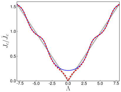
Figure 2: (Color online) Critical Josephson current $J_{c}$ (in units of $\tilde{J_{c}}$) of a step junction as a function of the chemical potential measured from the Dirac point energy $\Lambda$, see Eq. (29). The dashed red line shows the contribution of the propagating waves only, and the dotted black line is the asymptote for $|\Lambda|\gg 1$.

In Fig. 2 we plot the normalized critical current $J_{c}/\tilde{J_{c}}$ as a function of the rescaled energy,

$$\Lambda=\frac{\mu-\varepsilon_{0}^{yz}}{\hbar v_{F}^{yz}}\left(\frac{L}{\eta}\right)$$ (29)

Obviously, the critical current is dependent on $\eta=A_{1}/A_{2}$. Furthermore, we find a finite critical Josephson current for chemical potential at the Dirac point energy ($\Lambda=0$). By comparing this to the critical current due to propagating waves only (Fig. 2, dashed red line) we find that this finite current appears due to evanescent waves, i.e, due to imaginary $k_{z}$. This critical current at the Dirac point energy can be tuned by the fraction $\eta=A_{1}/A_{2}$: the larger $\eta$, the larger the critical current. The critical current for $\big{|}\Lambda\big{|}\gg 1$ follows the asymptote shown by the dotted black line in Fig. 2. The oscillations in the critical current can be considered as a negligible deviation in this limit.

Performing the same calculations for an edge junction yields

$$\varepsilon_{n} =\Delta_{0}\sqrt{(1-\tau_{n}\sin(\phi/2)^{2})},$$ (30)

$$\tau_{n} =-\frac{1}{\tan(\alpha)^{2}\sin(k_{zn}L)^{2}}.$$

Naturally, the result $\tau_{n}<0$ corresponds to $\varepsilon_{n}>\Delta_{0}$, implying the absence of Andreev bound states. The formation of Andreev bound states in the central region requires the presence of electrons with opposite spins in regions I and III. Due to spin momentum locking in the topological insulator and because the spins in region I and III lie in different planes, the formation of Andreev bound states is prohibited. The only possibility would be $k_{y}=0$, in which case the spin is along the $y$ direction. However, this is not allowed due to the boundary conditions: $k_{yn}=(n+1/2)\pi/W>0$. Thus, the contribution of the Andreev bound states to the Josephson current vanishes in these edge junctions.

III.2 SFS junctions

Again we focus on the step junction, since we can get the solutions for the planar junction by a change of variables (indices $yz\rightarrow xy$, $\eta=A_{1}/A_{2}\rightarrow 1$) and of the magnetization direction. First, we examine a junction with perpendicular magnetization and later on we will analyze the effects of the magnetization in all directions for the case, where the chemical potential is at the Dirac point energy.

III.2.1 Perpendicular magnetization ($m_{z}=0$ and $m_{y}=0$)

In the low-energy regime, i.e., for ($|\mu-\varepsilon_{0}^{yz}|\gg\varepsilon$) we can use $\kappa(-\varepsilon,-m_{z})\approx\kappa(\varepsilon,m_{z})\approx\frac{1}{\hbar v_{F}^{yz}\eta}\sqrt{m_{x}^{2}-(\mu-\varepsilon_{0}^{yz})^{2}+(k_{y}\hbar v_{F}^{yz})^{2}}=:\kappa$ resulting in the following energy:

$$\varepsilon=\Delta_{0}\sqrt{\frac{\kappa^{2}+k_{y}^{2}\sinh^{2}(\kappa L)-\kappa^{2}\sin^{2}(\phi/2)}{\kappa^{2}+(k_{y}^{2}+m_{x}^{2})\sinh^{2}(\kappa L)}}.$$ (31)

By introducing a finite width $W$ which quantizes $k_{y}\rightarrow k_{yn}$ ($n=0,1,2,\ldots$) and by using the “infinite mass” boundary condition the supercurrent due to the discrete spectrum is

$$J(\phi) =\frac{e\Delta_{0}}{\hbar}\frac{W}{2\pi}\int_{0}^{\infty}\frac{\kappa_{n}^{2}\sin(\phi)\varepsilon^{-1}_{n}(\phi)}{\kappa_{n}^{2}+(k_{yn}^{2}+m_{x}^{2})\sinh^{2}(\kappa_{n}L)}dk_{yn}.$$

The critical current can be calculated for different values of $q_{x}=\frac{m_{x}}{\hbar v_{F}^{yz}}\frac{L}{\eta}$, see Fig. 3. For $q_{x}=0$ the solutions of the normal step junction are recovered. The calculation shows that for $\Lambda=0$ and $q_{x}=0$ we get the critical current $J_{c}=0.21\tilde{J_{c}}$.

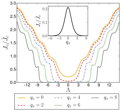
Figure 3: (Color online) Critical Josephson current $J_{c}$ (in units of $\tilde{J_{c}}$) of a ferromagnetic step junction as a function of $\Lambda$, see Eq. (29), for different values of $q_{x}=m_{x}L/(\hbar v_{F}^{yz}\eta)$. Inset: $J_{c}$ as a function of $q_{x}$ at the Dirac point ($\Lambda=0$).

Figure 3 shows that the magnetization $q_{x}$ can be used to tune the critical Josephson current. The stronger the magnetization, the larger the chemical potential needs to be, to result in a finite current. For large magnetization the finite Josephson current at the Dirac point ($\Lambda=0$) vanishes. This can be seen in the inset of Fig. 3 which shows the dependence of $J_{c}$ on $q_{x}$ at $\Lambda=0$.

At larger values of $\Lambda$ and $q_{x}$ we get a non-monotonic behavior, as it can be seen for $q_{x}=8$ in Fig. 3. We compare the values of $\Lambda$, where this non-monotonic behavior arises, to the scaled number of modes $N^{\prime}=NL/(W\eta)=\sqrt{\Lambda^{2}-q_{x}^{2}}/\pi$. When $\Lambda$ is small enough such that the curve is still monotonic, we find that $N^{\prime}<1$. We increase $\Lambda$ and just before the first local maximum of $J_{c}$, $N^{\prime}$ exceeds $1$. Similarly, just before the second local maximum $N$ increases further by 1.

When plotting the superconducting phase difference $\phi(J_{c})$ which maximizes the current $J$ against $\Lambda$, we find that this phase difference oscillates and the amplitude of the oscillations increase with $q_{x}$. This behavior is shown in Fig. 4. The crosses indicate the values of $\Lambda$ where $N^{\prime}$ becomes an integer. Again we see that by increasing $\Lambda$ the next integer value of $N^{\prime}$ is achieved just before the maximum of $\phi(J_{c})$. This correlation suggests that this non-monotonic behavior arises due to quantum interference of the new additional propagating mode and the already existing ones.

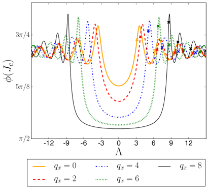
Figure 4: (Color online) Superconducting phase difference $\phi(J_{c})$ (which maximizes the current $J$) as a function of $\Lambda$, see Eq. (29), for different values of $q_{x}=m_{x}L/(\hbar v_{F}^{yz}\eta)$. The crosses indicate the values of $\Lambda$ at which the scaled number of modes $N^{\prime}=NL/(W\eta)=\sqrt{\Lambda^{2}-q_{x}^{2})}/\pi$ takes an integer value.

III.2.2 Chemical potential at the Dirac point energy ($\mu=\varepsilon_{0}^{yz}$)

In the limit $\mu=\varepsilon_{0}^{yz}$, it becomes possible to analytically examine arbitrary directions of the magnetization. If we assume $\sqrt{m_{x}^{2}+m_{z}^{2}}\gg\varepsilon$ then $\kappa(\varepsilon,-m_{z})\approx\kappa(0,-m_{z})=:\kappa(-m_{z})$ and $\kappa(-\varepsilon,m_{z})\approx\kappa(0,m_{z})=:\kappa(m_{z})$. Again we calculate the energy and find

$$\varepsilon =\frac{\Delta_{0}}{\sqrt{2}}\sqrt{1+\frac{1}{\eta^{2}}\left(k_{y}^{2}-\frac{m_{x}^{2}}{(\hbar v_{F}^{yz})^{2}}-\frac{m_{z}^{2}}{(\hbar v_{F}^{yz})^{2}}\right)f_{1}+f_{2}(\phi)},$$ (32)

$$f_{1} =\frac{\sinh(\kappa(m_{z})L)\sinh(\kappa(-m_{z})L)}{\kappa(m_{z})\kappa(-m_{z})\cosh[\kappa(m_{z})L]\cosh[\kappa(-m_{z})L]},$$

$$f_{2}(\phi) =\frac{\cos(2L\frac{m_{y}}{\hbar v_{F}^{yz}\eta}-\phi)}{\cosh[\kappa(m_{z})L]\cosh[\kappa(-m_{z})L]}.$$

The energy fulfills $\varepsilon\leq\Delta_{0}$. The current is calculated in the same way as before. We can see from Eq. (32) and in Fig. 5(c) that the magnetization $\frac{m_{y}}{\hbar v_{F}^{yz}\eta}$ leads to a phase shift in the Josephson current and thus does not influence the critical current. Furthermore, we observe from Fig. 5, that a magnetization in the $x$ direction (out of plane) suppresses the current more strongly than the magnetization in the $z$ direction (in plane and in the direction of transport).

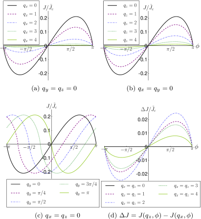
Figure 5: (Color online) Josephson current $J$ (in units of $\tilde{J_{c}}$) for the ferromagnetic step junction as a function of $\phi$ for different values of the magnetization parametrized by $q_{x,y,z}=m_{x,y,z}L/(\hbar v_{F}^{yz}\eta)$. The black line in (a), (b) and (c) corresponds to $q_{x}=q_{y}=q_{z}=0$. (d) shows the difference between the Josephson current of junctions with magnetization in $x-$ and $z-$direction ($\Delta J=J(q_{z},\phi)-J(q_{x},\phi)$).

IV Conclusion

We have conducted a detailed study of the Josephson effect on the surface of a topological insulator, using Bi₂Se₃ as a model system. The symmetries of the bulk crystal structure give rise to different Fermi velocities along the rotation symmetry axis and in the direction perpendicular to it. This manifests itself in a scaling factor in the critical Josephson current of the step junction when compared to the planar junction. This scaling appears in both normal and ferromagnetic topological insulator junctions. Interestingly, the contribution to the Josephson current from Andreev bound states vanishes for the edge junction. This suppression can be explained in terms of spin momentum locking, which prohibits the formation of Andreev bound states in the central region. In the ferromagnetic topological insulator step junction, we find that the critical Josephson current is suppressed for an out of plane magnetization as well as for a magnetization, which is in plane and in the direction of transport. A magnetization along the junction and perpendicular to the direction of transport leads to a finite Josephson current even when the phase difference of the superconductors is zero. Finally, we have obtained a non-monotonic critical Josephson current when the perpendicular magnetization and the chemical potential are sufficiently large, which was explained in terms of quantum interference of multiple modes in the junction. An experimental verification of this behavior (as shown in Fig. 3) could provide valuable insights into the transport mechanisms in these junctions.